Directed Nonabelian Sandpile Models on Trees

Abstract.

We define two general classes of nonabelian sandpile models on directed trees (or arborescences), as models of nonequilibrium statistical physics. Unlike usual applications of the well-known abelian sandpile model, these models have the property that sand grains can enter only through specified reservoirs.

In the Trickle-down sandpile model, sand grains are allowed to move one at a time. For this model, we show that the stationary distribution is of product form. In the Landslide sandpile model, all the grains at a vertex topple at once, and here we prove formulas for all eigenvalues, their multiplicities, and the rate of convergence to stationarity. The proofs use wreath products and the representation theory of monoids.

1. Introduction

Abelian sandpile models (ASMs) form one of the best understood classes of models in statistical physics motivated by the problem of understanding self-organized criticality [BTW87]. They can be defined for any graph, directed or otherwise. The models are stochastic and simple to describe. At any given time, each vertex of the graph contains a certain number of grains of sand less than its degree (outdegree in case of a directed graph). At each time step, a grain of sand is added to a random vertex. If the number of grains is still less than its degree, this is the new configuration. On the other hand if, as a result, the number of grains at that vertex becomes more than its degree, then the vertex is said to be unstable. It then topples, giving one grain to each of its neighbors along the edges. If more vertices become unstable as a result, they too topple. The model is defined by generators which describe the toppling for each vertex. The remarkable property of the abelian sandpile model is that these generators commute. This makes the models particularly amenable to computations of interest to physicists such as the distribution of avalanches. For physically motivated reviews of self-organized criticality and the abelian sandpile model, see [Dha90, IP98, Dha99a].

The model was also introduced around the same time by mathematicians under the name of chip-firing-games on graphs [BLS91]. ASMs on a graph are naturally related to other structures on the graph such as its sandpile group (also known as its critical group) [Big99], spanning trees and the Tutte polynomial [CLB03]. For mathematically oriented reviews of the abelian sandpile model, see [HLM⁺08] and [PS04, Appendix].

Nonequilibrium statistical physics largely deals with the study of systems in contact with (infinite) reservoirs. The classical example of such a system is a metal bar, both of whose ends are kept at different temperatures by means of baths (i.e. reservoirs). Although it is clear that heat will flow from the higher temperature reservoir to the lower one, specific statistical properties are not known. In fact, very few universal laws are known for such systems. It is therefore of great interest to understand toy examples of such dynamical systems in detail. We will model such systems by irreversible Markov chains, where there is a clear direction of the flow of particles.

We are interested in understanding real finite systems which interact with reservoirs only at the boundary, such as the metal bar example above. By that, we mean that we would not only like to understand the stationary distribution of these models, but also transient quantities, such as the time they take to reach the stationary distribution. We would also like our model to be generic in the sense that hopping rates for the particles are not chosen so that miraculous simplifications occur, and the model becomes tractable. In other words, we want our model to have “disordered” hopping rates. Lastly, we would like to prove rigorous statements about the behavior of the models. The standard ASM fails the reservoir criterion because grains are usually added to all sites, not just at the boundary. One could force grains to be added only at the reservoirs, but the resulting Markov chain could then fail to be ergodic. Even if that were not the case, all the dynamics happens because of grains being added externally and there is no intrinsic bulk motion, which is what we are interested in studying here.

There are exceptionally few Markov processes which satisfy all the conditions listed above and are not one-dimensional. Some examples known to us are the Manna model [Man91, Dha99b], the stochastic sandpile model [SD09], the asymmetric annihilation process [AS10], the asymmetric Glauber model [Ayy11] and the de-Bruijn process [AS13]. But these are also one-dimensional. There are very few nontrivial models of nonequilibrium statistical physics with reservoirs in higher dimensions where rigorous results are known, but most do not seem to be disordered; some examples are given in [Dha06]. We will present results for directed trees, which can be thought of as quasi two-dimensional objects since they can be embedded in the plane.

We introduce two new kinds of sandpile models on arbitrary rooted trees, which we call the Trickle-down sandpile model and the Landslide sandpile model. Although neither model is abelian, they have beautiful properties. The stationary distribution of the Trickle-down sandpile model has a product form, which means that the height distributions are independent and there are no correlations. The Landslide sandpile model has a remarkably simple formula for the eigenvalues of the transition matrix and their multiplicities. It also has a fast mixing time (i.e. convergence to steady state) which is approximately proportional to the square of the size of the rooted tree. The underlying basis for this fact, explained below, is the notion of ${\mathscr{R}}$-triviality. This idea is a precise mathematical formulation of forgetfulness of the initial distribution for a Markov chain. Some other examples of “${\mathscr{R}}$-trivial” statistical physical models are given in [AS10, Ayy11, AS13]. The stationary distribution of the Landslide sandpile model is nontrivial. It would be very interesting to calculate physically relevant quantities such as average avalanche sizes, their exponents, and various correlation functions.

A novel element of this paper is also our techniques. Influential work of Diaconis [Dia88] and others, going back to the eighties, has made the character and representation theory of finite groups extremely relevant to the analysis of Markov chains. In groundbreaking work, Bidigare, Hanlon and Rockmore [BHR99] introduced the new technique of monoid representation theory into the study of Markov chains and showed how this theory leads to an elegant analysis of the eigenvalues for Markov chains like the Tsetlin library and riffle-shuffling. This approach was further developed by Brown and Diaconis [BD98], Brown [Bro00], Björner [Bjö09, Bjö08], and Chung and Graham [CG12]. The types of monoids used in this theory are fairly restrictive and Diaconis asked in his 1998 ICM address how far the monoid techniques can be pushed [Dia98]. The third author initiated a theory for random walks on more general monoids in [Ste06, Ste08]. The first two authors in collaboration with Klee used these techniques to analyze Markov chains associated to Schützenberger’s promotion operators on posets [AKS14]. A multitude of further examples is presented in [ASST14]. The results of these papers, and this one, rely on the representation theory of the important class of ${\mathscr{R}}$-trivial monoids [Eil76]. A key feature of ${\mathscr{R}}$-trivial monoids is that any matrix representation of an ${\mathscr{R}}$-trivial monoid can be triangularized. The point here is that eigenvalues for upper triangular matrices are particularly easy to compute.

Another new feature in this paper is the use of self-similarity in the wreath product of monoids to analyze Markov chains, and in particular to compute stationary distributions. Such techniques have already been used to great effect for analyzing random walks and the spectrum of the discrete Laplacian on infinite groups [GŻ01, GNS00, KSS06], but they have never before been used in the monoid context or for finite state Markov chains.

As a side remark, we note that ASMs have also been studied from the monoid point of view in [Tou05].

The paper is organized as follows. In Section 2 we introduce both variants of the directed nonabelian sandpile model and state the main results. Section 3 reformulates the directed nonabelian sandpile model in terms of wreath products. In Section 4 we present the proofs for the stationary distributions using the wreath product approach. For the Trickle-down sandpile model we provide another proof using a master equation; it becomes clear that the wreath product approach is superior in this setting. Section 5 gives a proof of ${\mathscr{R}}$-triviality for the monoid of the Landslide sandpile model, which yields the statements about the eigenvalues. We also prove the rate of convergence.

Acknowledgments

All the authors would like to thank ICERM, where part of this work was performed, for its hospitality. AS was partially supported by NSF grants DMS–1001256, OCI–1147247, and a grant from the Simons Foundation (#226108 to Anne Schilling). This work was partially supported by a grant from the Simons Foundation (#245268 to Benjamin Steinberg).

We would like to thank D. Dhar, F. Bergeron and an anonymous referee for comments.

This research was driven by computer exploration using Maple${}^{{\text{T}M}}$, Sage [S⁺13] and Sage-combinat [SCc08]. The Sage code is available by request and the Maple package NonabelianSandpiles.maple can be downloaded from the arXiv source.

2. Definition of models and statement of results

A tree is a graph without cycles. An arborescence, or out-tree, is a directed graph with a special vertex called the root such that there is exactly one directed path from any vertex to the root. Note that an arborescence on $n$ vertices has exactly $n-1$ directed edges. Vertices of degree one in an arborescence are called leaves. An example is given in Figure 1.

Figure 1. An arborescence with leaves a, g, h, j, k and root ${\mathsf{r}}$

We will now informally define our nonabelian sandpile models on arborescences. These models will be considered as (discrete-time) Markov chains. This is a very well-developed theory, see [LPW09], for instance. A Markov chain can be thought of as a random walk on an appropriate graph. For our purposes, we will need the following facts. If the graph is strongly connected, then the Markov chain is recurrent, meaning one can get from any configuration to any other configuration. If in addition, there is a single loop in the graph, then the chain is aperiodic and it converges exponentially fast to its unique stationary distribution. The stationary distribution is, in our convention, the right eigenvector with eigenvalue 1 of the transition matrix. The eigenvector is normalized so that the sum of the entries is 1. We call the normalization factor, albeit with some abuse of terminology, the partition function.

We will define two Markov chains on configurations of arborescences. In both models, each vertex has a threshold, which is the maximum number of sand grains that it can accommodate. Sand enters from the leaves with a certain probability depending on the leaf, one at a time, flow down the tree, and leave at the root. Moreover, the interior vertices can topple with a certain probability. The difference in the models is in the way in which the interior vertices topple.

In the Trickle-down sandpile model, the toppling at a vertex $v$ affects only one grain of sand at that vertex. That grain moves from $v$, along the directed path to the root ${\mathsf{r}}$, until it finds a vertex $w$ which does not have its threshold number of sand grains, and settles there. In other words, the number of sand grains at $v$ reduces by 1 and those at $w$ increases by 1. If no such $w$ exists (i.e. all vertices along the path are filled to capacity), the sand grain exits the arborescence at the root.

In the Landslide sandpile model, the toppling at $v$ removes all the grains of sand at that vertex. These grains are then transferred systematically to the vertices along the path from $v$ to ${\mathsf{r}}$. If there are still some grains remaining at the end, these grains leave the arborescence at the root. Note that if the vertex being toppled is the root ${\mathsf{r}}$, then all the sand grains at ${\mathsf{r}}$ exit the arborescence.

Figure 2. Arborescence $\mathcal{T}_{3}$ for Example 2.1

Example 2.1.

Let $\mathcal{T}_{3}$ be the arborescence consisting of two leaves and a root, shown in Figure 2, with all thresholds equal to 1. Note that both the Trickle-down sandpile model and the Landslide sandpile model are equivalent in this case. There are 8 states in the Markov chain, which are given by binary vectors of size 3, denoting the number of grains in vertices $a,b,{\mathsf{r}}$ in that order. Let the probability for grains entering at vertices $a$ and $b$ be $y_{a}$ and $y_{b}$, respectively, and the probability for toppling at the nodes be $x_{a},x_{b}$ and $x_{\mathsf{r}}$, with $y_{a}+y_{b}+x_{a}+x_{b}+x_{\mathsf{r}}=1$. The graph for the Markov chain is given in Figure 3

• 

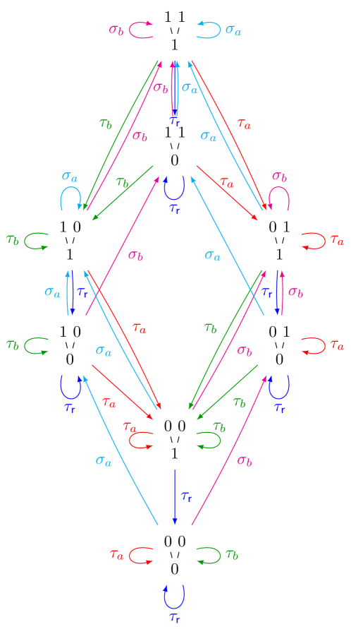
Figure 3. The graph $G_{\theta}=G_{\tau}$ of the Markov chain with unit thresholds for the arborescence of Example 2.1.

Our convention for the transition matrix for the chain $M$ is that $M_{i,j}$ is the probability of going from state $j$ to state $i$ so that the column sums are 1. The rows and columns of $M$ are labelled by the states in lexicographic order, that is $\{000,001,010,011,100,101,110,111\}$,

$$M=\left(\begin{array}[]{cccccccc}*&x_{{{{\mathsf{r}}}}}&0&0&0&0&0&0\\ \vskip 6.0pt plus 2.0pt minus 2.0pt\cr 0&*&x_{{b}}&x_{{b}}&x_{{a}}&x_{{a}}&0&0\\ \vskip 6.0pt plus 2.0pt minus 2.0pt\cr y_{{b}}&0&*&x_{{{{\mathsf{r}}}}}&0&0&0&0\\ \vskip 6.0pt plus 2.0pt minus 2.0pt\cr 0&y_{{b}}&y_{{b}}&*&0&0&x_{{a}}&x_{{a}}\\ \vskip 6.0pt plus 2.0pt minus 2.0pt\cr y_{{a}}&0&0&0&*&x_{{{{\mathsf{r}}}}}&0&0\\ \vskip 6.0pt plus 2.0pt minus 2.0pt\cr 0&y_{{a}}&0&0&y_{{a}}&*&x_{{b}}&x_{{b}}\\ \vskip 6.0pt plus 2.0pt minus 2.0pt\cr 0&0&y_{{a}}&0&y_{{b}}&0&*&x_{{{{\mathsf{r}}}}}\\ \vskip 6.0pt plus 2.0pt minus 2.0pt\cr 0&0&0&y_{{a}}&0&y_{{b}}&y_{{a}}+y_{{b}}&*\end{array}\right),$$

where the entries on the diagonal are such that column sums are 1. One can verify that the nonzero entries in $M$ precisely correspond to the directed arrows is Figure 3.

The stationary distribution $\mathbb{P}$ is then the column (right) eigenvector of $M$ with eigenvalue 1, properly normalized. The probability for each state is then given by

$$\mathbb{P}(0,0,0) ={\frac{x_{{a}}x_{{b}}x_{{{{\mathsf{r}}}}}}{Z}},\quad\mathbb{P}(0,0,1)={\frac{x_{{a}}x_{{b}}\left(y_{{a}}+y_{{b}}\right)}{Z}},$$

$$\mathbb{P}(0,1,0) ={\frac{x_{{a}}y_{{b}}x_{{{{\mathsf{r}}}}}}{Z}},\quad\mathbb{P}(0,1,1)={\frac{x_{{a}}y_{{b}}\left(y_{{a}}+y_{{b}}\right)}{Z}},$$

$$\mathbb{P}(1,0,0) ={\frac{y_{{a}}x_{{b}}x_{{{{\mathsf{r}}}}}}{Z}},\quad\mathbb{P}(1,0,1)={\frac{y_{{a}}x_{{b}}\left(y_{{a}}+y_{{b}}\right)}{Z}},$$

$$\mathbb{P}(1,1,0) ={\frac{y_{{a}}y_{{b}}x_{{{{\mathsf{r}}}}}}{Z}},\quad\mathbb{P}(1,1,1)={\frac{y_{{a}}y_{{b}}\left(y_{{a}}+y_{{b}}\right)}{Z}},$$

where $Z$ is the normalization factor, often called the nonequilibrium partition function,

$$Z=\left(x_{{a}}+y_{{a}}\right)\left(x_{{b}}+y_{{b}}\right)\left(y_{{a}}+y_{{b}}+x_{{{{\mathsf{r}}}}}\right).$$

One can see that this is of product form. This property will generalize to the Trickle-down sandpile model for all arborescences.

The eigenvalues of $M$ are given by

$$0,x_{{a}},x_{{{{\mathsf{r}}}}},x_{{b}},x_{{a}}+x_{{b}},y_{{a}}+x_{{a}}+x_{{{{\mathsf{r}}}}},$$

$$y_{{b}}+x_{{b}}+x_{{{{\mathsf{r}}}}},x_{{b}}+x_{{{{\mathsf{r}}}}}+y_{{b}}+y_{{a}}+x_{{a}}=1.$$

This property of the eigenvalues being partial sums of the probabilities will persist for the Landslide sandpile model in general.

The plan for the rest of this section is as follows. We will first define the state space of our models in Section 2.1. The Trickle-down sandpile model is defined in Section 2.2, where we also state the stationary distribution for this model. The Landslide sandpile model is introduced in Section 2.3 together with its stationary distribution and precise formulas for the eigenvalues of the transition matrix. In Section 2.4 we state the rate of convergence and mixing time for the Landslide sandpile model. Finally in Section 2.5, we discuss the specialization of the Markov chains to the case when the tree is just a one-dimensional line.

2.1. Arborescences

Let $V$ be the vertex set of the arborescence. We only consider arborescences with finitely many vertices. The special root vertex is denoted by ${\mathsf{r}}$.

To each vertex $v\in V$, we associate a threshold $T_{v}$. The state space of our Markov chain is defined to be

(2.1) $$\Omega=\Omega(\mathcal{T}):=\{(t_{v})_{v\in V}\mid 0\leq t_{v}\leq T_{v}\}.$$

In other words, at vertex $v$ there can be at most $T_{v}$ grains. We gather all thresholds in a tuple as $T=(T_{v})_{v\in V}$. The arborescence with its vertices $V$, edges $E$ and thresholds $T$ is denoted by $\mathcal{T}=(V,E,T)$. An example of a configuration $t\in\Omega(\mathcal{T})$ is given in Figure 4.

Figure 4. A configuration for the arboresence from Figure 1 with all thresholds $T_{v}=2$.

The Markov chain is defined by certain toppling and source operators on the state space. We associate a toppling operator $\theta_{v}\colon\Omega\to\Omega$ to each vertex $v\in V$ for the Trickle-down sandpile model (respectively $\tau_{v}\colon\Omega\to\Omega$ for the Landslide sandpile model). They topple grains from vertex $v$ along the unique outgoing edge. (Here we assume that an outgoing edge is attached to the root ${\mathsf{r}}$). The precise definitions are stated in the next subsections. In addition, let $L$ be the set of leaves of the arborescence. The source operators $\sigma_{\ell}\colon\Omega\to\Omega$ for $\ell\in L$ are certain operators adding grains at the leaves.

Let $\{x_{v},y_{\ell}\mid v\in V,\ell\in L\}$ be a probability distribution on toppling and source operators, that is, $x_{v}$ is the probability of choosing $\theta_{v}$ (respectively $\tau_{v}$) and $y_{\ell}$ is the probability of choosing $\sigma_{\ell}$. We assume that

1. $0<x_{v},y_{\ell}\leq 1$

2. $\sum_{v\in V}x_{v}+\sum_{\ell\in L}y_{\ell}=1$

to make it into a proper probability distribution. But in principle these constraints can be relaxed. This defines for us Markov chains as random walks on graphs whose states are the elements of $\Omega$ and whose weighted edges are given by the toppling and source operators.

Next we define both models in detail.

2.2. Trickle-down sandpile model

For a vertex $v\in V$ let

(2.2) $$v^{\downarrow}=(v=v_{0}\to v_{1}\to\cdots\to v_{a}={\mathsf{r}})$$

be the path from $v$ to the root ${\mathsf{r}}$; we also use this notation for the set of vertices of the path (the downset of $v$).

Source operator: For each leaf $v\in L$, we define a source operator $\sigma_{v}\colon\Omega\to\Omega$ as follows. As stated before, the source operator follows the path $v^{\downarrow}$ from the leaf $v$ to the root ${\mathsf{r}}$ and adds a grain to the first vertex along the way that has not yet reached its threshold, if such a vertex exists. The precise definition (retaining the notation of (2.2)) is: given $t=(t_{w})_{w\in V}\in\Omega$, define $\sigma_{v}(t)=t^{\prime}$ as follows. Let $k\geq 0$ be smallest such that $t_{v_{k}}\neq T_{v_{k}}$. In other words, $t_{v_{0}}=T_{v_{0}},\ldots,t_{v_{k-1}}=T_{v_{k-1}}$, but $t_{v_{k}}<T_{v_{k}}$. Then $t_{w}^{\prime}=t_{w}$ for all $w\in V$ except for $w=v_{k}$, and $t_{v_{k}}^{\prime}=t_{v_{k}}+1$. If no such $k$ exists, then $t^{\prime}=t$.

Topple operator: For each vertex $v\in V$, we define a topple operator $\theta_{v}\colon\Omega\to\Omega$. Intuitively, $\theta_{v}$ takes a grain from vertex $v$ and adds it to the first possible site along the path from $v$ to the root. If there is no available site, the grain drops out after the root. Let us give the formal definition. Let $t=(t_{w})_{w\in V}\in\Omega$ and put $\theta_{v}(t)=t^{\prime}$ defined as follows. Consider the path $v^{\downarrow}$ as in (2.2). If $t_{v}=0$, then $\theta_{v}(t)=t$. Otherwise $t_{v}>0$ and let $k\geq 1$ be smallest such that $t_{v_{k}}\neq T_{v_{k}}$. In other words, $t_{v_{1}}=T_{v_{1}},\ldots,t_{v_{k-1}}=T_{v_{k-1}}$, but $t_{v_{k}}<T_{v_{k}}$. Then $t_{w}^{\prime}=t_{w}$ except $t_{v}^{\prime}=t_{v}-1$ and $t_{v_{k}}^{\prime}=t_{v_{k}}+1$. If no such $k$ exists, then $t_{w}^{\prime}=t_{w}$ except $t_{v}^{\prime}=t_{v}-1$.

In particular for $v={\mathsf{r}}$ the root, we have $t_{\mathsf{r}}^{\prime}=\max\{0,t_{\mathsf{r}}-1\}$ and all other $t_{w}$ are unchanged.

Examples for the source and topple operators for the Trickle-down sandpile model are given in Figures 5 and 6, respectively.

$\sigma_{j}:$

$\mapsto$

$\sigma_{g}:$

$\mapsto$

Figure 5. Example of source operator actions on states in $\Omega(\mathcal{T})$ for $\mathcal{T}$ as in Figure 1.

$\theta_{k}:$

$\mapsto$

$\theta_{g}:$

$\mapsto$

Figure 6. Example of topple operator actions of the Trickle-down sandpile model on states in $\Omega(\mathcal{T})$ for $\mathcal{T}$ as in Figure 1.

Proposition 2.2.

The directed graph $G_{\theta}$ whose vertex set is $\Omega$ and whose edges are given by the operators $\sigma_{\ell}$ for $\ell\in L$ and $\theta_{v}$ for $v\in V$ is strongly connected and the corresponding Markov chain is ergodic.

We defer the proof of Proposition 2.2 until Section 2.3. Examples of $G_{\theta}$ are given in Figure 3 and Figure 8.

For $v\in V$, let $L_{v}$ be the set of all sources $\ell\in L$ whose downset $\ell^{\downarrow}$ contains $v$. More precisely,

$$L_{v}:=\{\ell\in L\mid v\in\ell^{\downarrow}\}.$$

Moreover, let $Y_{v}:=\sum_{\ell\in L_{v}}y_{\ell}$. For $v\in V$ and $0\leq h\leq T_{v}$, let

(2.3) $$\rho_{v}(h):=\dfrac{Y_{v}^{h}\;x_{v}^{T_{v}-h}}{\sum_{i=0}^{T_{v}}Y_{v}^{i}\;x_{v}^{T_{v}-i}}.$$

Then the following theorem completely describes the stationary distribution.

Theorem 2.3.

The stationary distribution of the Trickle-down sandpile Markov chain defined on $G_{\theta}$ is given by the product measure

(2.4) $$\mathbb{P}(t)=\prod_{v\in V}\rho_{v}(t_{v}).$$

A proof of Theorem 2.3 using master equations is given in Section 4.1. An alternative proof with an algebraic flavor is presented in Section 4.2.

The theorem implies that the random variables giving the number of grains at vertex $v$ and at vertex $u$ are independent if we sample from the stationary distribution, regardless of where $u$ and $v$ are located on the tree.

Recall that the (nonequilibrium) partition function of a Markov chain is the least common denominator of the stationary probabilities. The following is an immediate corollary of Theorem 2.3.

Corollary 2.4.

The partition function $Z_{\theta}$ of the Trickle-down sandpile Markov chain defined on $G_{\theta}$ is

$$Z_{\theta}=\prod_{v\in V}\bigl{(}\sum_{i=0}^{T_{v}}Y_{v}^{i}x_{v}^{T_{v}-i}\bigr{)}.$$

2.3. Landslide sandpile model

In this model, we define the paths $v^{\downarrow}$ from a vertex $v\in V$ to the root ${\mathsf{r}}$ as in (2.2) and the source operators as in Section 2.2. The topple operator on the other hand will topple the entire site instead of just a single grain.

Topple operator: For each vertex $v\in V$, we define a topple operator $\tau_{v}\colon\Omega\to\Omega$. As stated before, $\tau_{v}$ empties site $v$ and transfers all grains at site $v$ to the first available sites on the path from $v$ to the root. If there are still grains remaining, they exit the system from the root. Formally, we can define $\tau_{v}=\theta_{v}^{T_{v}}$, that is $\tau_{v}$ is defined to be applying $\theta_{v}$ as many times as the threshold $T_{v}$ of $v$.

Examples for the topple operators for the Landslide sandpile model are given in Figure 7.

$\tau_{k}:$

$\mapsto$

$\tau_{g}:$

$\mapsto$

Figure 7. Example of topple operator actions of the Landslide sandpile model on states in $\Omega(\mathcal{T})$ for $\mathcal{T}$ as in Figure 1.

Remark 2.5.

If the thresholds are all one, that is, $T_{v}=1$ for all $v\in V$, then the Trickle-down and Landslide sandpile models are equivalent.

Remark 2.6.

The directed nonabelian sandpile models can also be defined recursively by successively removing leaves. This approach is taken in Sections 3 through 5 when we prove the stationary distributions and ${\mathscr{R}}$-triviality of the underlying monoid.

Proposition 2.7.

The directed graph $G_{\tau}$ whose vertex set is $\Omega$ and whose edges are given by the operators $\sigma_{\ell}$ for $\ell\in L$ and $\tau_{v}$ for $v\in V$ is strongly connected and the corresponding Markov chain is ergodic.

We prove Propositions 2.2 and 2.7 simultaneously.

Proof.

First we prove that $G_{\tau}$ is strongly connected. By applying the operators $\tau_{v}$ with $v\in V$ sufficiently often, we can transform any state to the zero state $(0)_{v\in V}$.

To go from $(0)_{v\in V}$ to any $t\in\Omega$ we use the following strategy. Let $\ell$ be a leaf and consider the path (2.2). Suppose that $t^{\prime}$ satisfies $t^{\prime}_{v_{0}}=t^{\prime}_{v_{1}}=\cdots=t^{\prime}_{v_{k}}=0$. Then $\tau_{v_{k-1}}\cdots\tau_{v_{1}}\tau_{v_{0}}\sigma_{\ell}^{t_{k}}t^{\prime}$ agrees with $t^{\prime}$ at each vertex except $v_{k}$, which will now have $t_{k}$ grains. Thus applying successively operations of this form, starting with $k=a$, we can transform $(0)_{v\in V}$ to a vector which agrees with $t$ on all vertices of $\ell^{\downarrow}$ and has $0$ at all remaining vertices. Then proceeding from leaf to leaf, we can eventually reach the vector $t$. Thus $G_{\tau}$ is strongly connected. Observing that $\tau_{v}=\theta_{v}^{T_{v}}$ it immediately follows that $G_{\theta}$ is also strongly connected.

Both chains are aperiodic because $\tau_{v}$ and $\theta_{v}$ fix $(0)_{v\in V}$ and so both digraphs contain loop edges. ∎

Since, when all thresholds are one, the Landslide sandpile model is the same as the Trickle-down sandpile model (see Remark 2.5), Figure 3 and Figure 8 also serve as examples for $G_{\tau}$.

The stationary distribution in this model is not a product measure in general. However, it is in one special case. Let

(2.5) $$\mu_{v}(h):=\begin{cases}\frac{\displaystyle Y_{v}^{h}x_{v}}{\displaystyle(Y_{v}+x_{v})^{h+1}}&\text{if }h<T_{v},\\ \\ \frac{\displaystyle Y_{v}^{T_{v}}}{\displaystyle(Y_{v}+x_{v})^{T_{v}}}&\text{if }h=T_{v},\end{cases}$$

where as in Section 2.2 we have $Y_{v}=\sum_{\ell\in L_{v}}y_{\ell}$. It is easy to check that $\displaystyle\sum_{h=1}^{T_{v}}\mu_{v}(h)=1$ for all $v\in V$.

Theorem 2.8.

Let $T_{v}=1$ for all $v\in V$, $v\neq{\mathsf{r}}$ and $T_{\mathsf{r}}=m$ for some positive integer $m$. Then the stationary distribution of the Landslide sandpile model defined on $G_{\tau}$ is given by the product measure

$$\mathbb{P}(t)=\prod_{v\in V}\mu_{v}(t_{v}).$$

The proof of Theorem 2.8 is given in Section 4.2. The following is an immediate consequence of Theorem 2.8.

Corollary 2.9.

Let $T_{v}=1$ for all $v\in V$, $v\neq{\mathsf{r}}$ and $T_{\mathsf{r}}=m$. Then the partition function $Z_{\tau}$ of the Landslide sandpile model defined on $G_{\tau}$ is

$$Z_{\tau}=\prod_{v\in V}(Y_{v}+x_{v})^{T_{v}}.$$

The eigenvalues for the transition matrices for the Landslide sandpile model Markov chain are given by a very elegant formula. Let $M_{\tau}$ be the transition matrix for the Markov chain. For $S\subseteq V$, let

(2.6) $$y_{S}=\sum_{\ell\in L,\ell^{\downarrow}\subseteq S}y_{\ell}\;\text{ and }\;x_{S}=\sum_{v\in S}x_{v},$$

where $\ell^{\downarrow}$ is the set of all vertices on the path from $\ell$ to ${\mathsf{r}}$.

Theorem 2.10.

The characteristic polynomial of $M_{\tau}$ is given by

$$\det(M_{\tau}-\lambda\mathbbm{1})=\prod_{S\subseteq V}(\lambda-y_{S}-x_{S})^{T_{S^{c}}},$$

where $S^{c}=V\setminus S$ and $T_{S}=\prod_{v\in S}T_{v}$.

We defer the proof of this theorem to Section 5.2, where monoid theoretic techniques are used.

2.4. Rate of convergence for the Landslide sandpile model

For the Landslide sandpile model, we can make explicit statements about the rate of convergence to stationarity and mixing times. Let $P^{k}$ be the distribution after $k$ steps. The rate of convergence is the total variation distance from stationarity after $k$ steps, that is,

$$||P^{k}-\pi||=\frac{1}{2}\sum_{t\in\Omega}|P^{k}(t)-\pi(t)|$$

where $\pi$ is the stationary distribution.

Theorem 2.11.

Define $p_{x}:=\min\{x_{v}\mid v\in V\}$ and $n:=|V|$. Then, as soon as $k\geq(n-1)/p_{x}$, the distance to stationarity of the Landslide sandpile model satisfies

$$||P^{k}-\pi||\leq\exp\left(-\frac{(kp_{x}-(n-1))^{2}}{2kp_{x}}\right)\,.$$

The proof of Theorem 2.11 is given in Section 5.3. Note that the bound does not depend on the thresholds.

The mixing time [LPW09] is the number of steps $k$ until $||P^{k}-\pi||\leq e^{-c}$ (where different authors use different conventions for the value of $c$). Using Theorem 2.11 we require

$$(kp_{x}-(n-1))^{2}\geq 2kp_{x}c\,,$$

which shows that the mixing time is at most $\frac{2(n+c-1)}{p_{x}}$. If the probability distribution $\{x_{v},y_{\ell}\mid v\in V,\ell\in L\}$ is uniform, then $p_{x}$ is of order $1/n$ and the mixing time is of order at most $n^{2}$.

The above bounds could be further improved.

2.5. The one-dimensional models

When the arborescence is a line, both the Trickle-down sandpile model and the Landslide sandpile model simplify considerably. First of all, the notation can be made more concrete. We may assume that the set of vertices $V$ is $\{1,\dots,n\}$, which are labeled consecutively from the unique source $1$ to the root $n$. The threshold vector $T$ is considered as an $n$-tuple of positive integers. We denote the probability of the source operator $\sigma_{1}$ by $y=y_{1}$ and the probability of toppling at vertex $i$ by $x_{i}$ in both models for the sake of consistency. Note that $Y_{i}=y$ for all $i$. Examples of the one-dimensional models of length 2 and 3 are illustrated in Figure 8.

The Trickle-down sandpile model can be thought of as a natural variant of the totally asymmetric simple exclusion process (TASEP), whose stationary distribution was computed exactly in [DEHP93]. In the case when all the thresholds are equal and all rates 1, this model has been introduced under the name of the drop-push process on the ring [SRB96]. The model has been generalized to include arbitrary thresholds and probabilities, but still on the ring [TB97]. It is also related to the $m$-TASEP, which has been studied on $\mathbb{Z}$ [SW98]. Toppling operations on partitions and compositions have also been studied from an order-theoretic point of view [GMP02].

• 

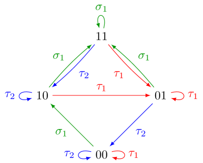
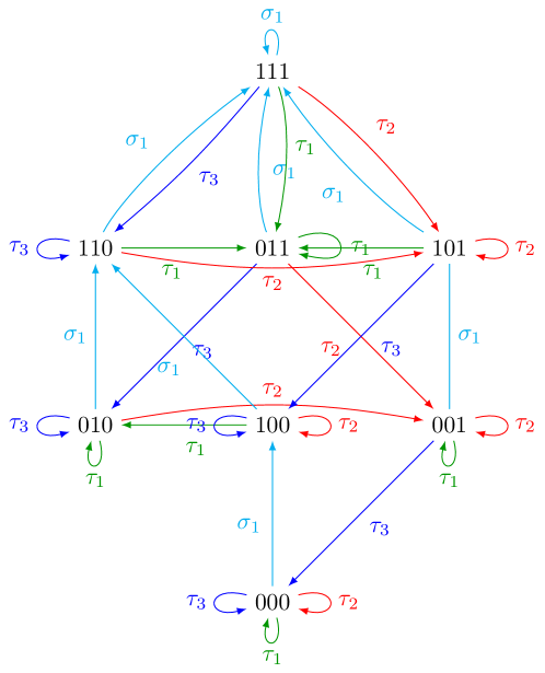
Figure 8. The graph $G_{\theta}=G_{\tau}$ of the Markov chain with unit thresholds for the line $1\rightarrow 2$, the line $1\rightarrow 2\rightarrow 3$, respectively.

The stationary distribution for the Trickle-down sandpile model is a product measure for all $n$ and any transition probabilities, unlike for the TASEP. This follows from Theorem 2.3.

Corollary 2.12.

The stationary distribution of the Markov chain defined by $G_{\theta}$ is a product measure,

$$\mathbb{P}(v)=\prod_{j=1}^{n}\rho_{j}(v_{j}),$$

where $\rho$ is defined in (2.3).

The Landslide sandpile model is a natural model for the transport of large self-organizing objects such as macromolecules. These have been considered in biophysics since at least the 1960s [MGP68, MG69]. However, no exact results are known for such models to the best of our knowledge.

For nonequilibrium statistical systems, it is very rare to have a concrete example of Markov chains where all the eigenvalues of the transition matrix are known for any choice of rates. Some examples are given in [AS10, Ayy11, AS13]. For models related to abelian sandpiles, there are some conjectures about eigenvalues in [SD09, Dha99b].

Corollary 2.13.

The characteristic polynomial of $M_{\tau}$ on $[n]$ is given by

$$\det(M_{\tau}-\lambda\mathbbm{1})=(\lambda-x_{0}-x_{[n]})\prod_{\phi\subseteq S\subsetneq[n]}(\lambda-x_{S})^{T_{S^{c}}},$$

where $S^{c}=[n]\setminus S$, $x_{S}=\sum_{i\in S}x_{i}$ and $T_{S}=\prod_{i\in S}T_{i}$.

The stationary distribution of the Landslide sandpile model is not a product measure, but it still has some interesting structure. The following conjecture follows from looking at the partition function for various thresholds vectors up to size 6. We have a similar conjecture for Landslide sandpile model on trees, but is much more complicated to write down.

Conjecture 2.14.

Given the threshold vector $T$ for the Landslide sandpile model on $[n]$, let $k:=\min\{i\in[n]\mid T_{i}>1\}$. Then, the partition function $Z_{\tau}$ is given by

$$Z_{\tau}=\prod_{i=1}^{k-1}(y_{1}+x_{i})^{T_{i}}\prod_{\phi\subsetneq S\subseteq\{k,\dots,n\}}(y_{1}+x_{S})^{T_{\min\{i\mid i\in S\}}}.$$

One can check that this matches Corollary 2.9 when $k=n$, that is, when the thresholds are one everywhere except at the root.

3. Monoids for sandpile models

We will now show how the two variants of the sandpile model can be modeled via the wreath product of left transformation monoids [Eil76]. This section is particularly inspired by the theory of self-similar groups and automaton groups [GNS00, GŻ01, KSS06, Nek05]. The wreath product formulation makes it possible to give a simple proof of the stationary distribution for the Trickle-down sandpile model and to prove ${\mathscr{R}}$-triviality of the underlying monoid of the Landslide sandpile model. Using the results in [Ste06, Ste08] then yields our results for eigenvalues and multiplicities.

This section is organized as follows. In Section 3.1 we review definitions and concepts from monoid theory that are necessary to prove our theorems. In Section 3.2 we present generalities on wreath products. The two variants of the nonabelian sandpile model are reformulated in Section 3.3 in terms of the wreath product. This formulation will be used in Sections 4 and 5 to prove our statements about the stationary distribution, eigenvalues, and rates of convergence.

3.1. Posets and monoids

A partially ordered set (poset) $P$ is a set with a reflexive, transitive and asymmetric relation $\leq$. The set of vertices of an arborescence is partially ordered by $v\leq w$ if there is a path from $w$ to $v$. With this ordering the root is the smallest element and the leaves are the maximal elements. An upset $U$ in a poset $P$ is a subset such that $x\in U$ and $y\geq x$ implies $y\in U$. A downset $D$ is defined dually, $x\in D$ and $y\leq x$ implies $y\in D$. Denote by $x^{\downarrow}=\{y\in P\mid y\leq x\}$. (This is consistent with the usage in (2.2).) A poset is called a lattice if it has a greatest element, a least element and any two elements have a least upper bound (join) and a greatest lower bound (meet). For a finite poset to be a lattice it is enough for it to have a greatest element and binary meets.

A finite monoid $M$ is a finite set with an associative multiplication and an identity element $\varepsilon$. If $X\subseteq M$, then the submonoid $\langle X\rangle$ generated by $X$ is the smallest submonoid of $M$ containing $X$. It consists of all (possibly empty) iterated products of elements of $X$. Basic references for the theory of monoids are [CP61, How95, Hig92]. Books specializing in finite monoids are [Eil76, KRT68, Alm94, RS09, Pin86].

An action of a monoid $M$ on a set $\Omega$ is a mapping $M\times\Omega\to\Omega$, written as juxtaposition, such that $\varepsilon x=x$ and $(mm^{\prime})x=m(m^{\prime}x)$ for all $m,m^{\prime}\in M$ and $x\in\Omega$. Given a probability $\mathbb{P}$ on $M$, we can define a Markov chain $\mathcal{M}$ on $\Omega$ by defining the transition probability from $x$ to $y$ to be the probability that $mx=y$ if $m$ is distributed according to $\mathbb{P}$. The so-called “random mapping representation” of a Markov chain [LPW09] asserts that all finite state Markov chains can be realized in this way.

The monoid point of view brings a new perspective: the generators of the monoid act on itself on both sides. This gives rise to the left (respectively right) Cayley graph: its vertex set is $M$, and for $m,m^{\prime}\in M$ and $g$ a generator, there is an edge $m\stackrel{{\scriptstyle g}}{{\mapsto}}m^{\prime}$ whenever $m^{\prime}=gm$ (respectively $m^{\prime}=mg$). See Figures 9 and 10 for examples. Notice that the left Cayley graph contains the graph of the Markov chain as its lowest strongly connected component comparing with Figure 8 (a usual feature; the elements of this component are the constant functions) and is therefore no simpler to study than the Markov chain itself. On the other hand, the right Cayley graph is acyclic! This is a strong feature, called ${\mathscr{R}}$-triviality, which we are going to introduce next and which is used extensively throughout the paper. As we will show in Section 5.1, the monoids associated to the Landslide sandpile model introduced on this paper are ${\mathscr{R}}$-trivial.

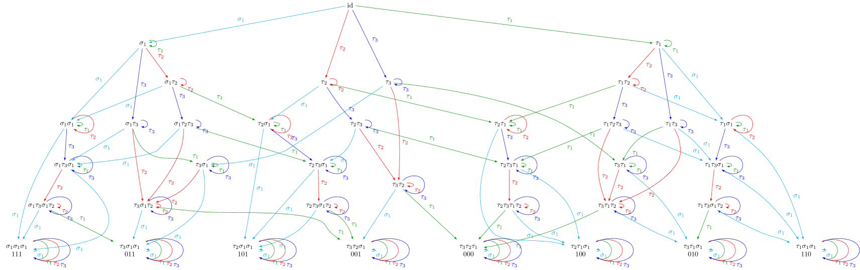
Figure 9. The right Cayley graph of the monoid for the one-dimensional Landslide sandpile model with three sites as in Figure 8. Each vertex displays a reduced word for the corresponding element $m$ of the monoid; if $m$ is a constant function, the value of this function is appended.

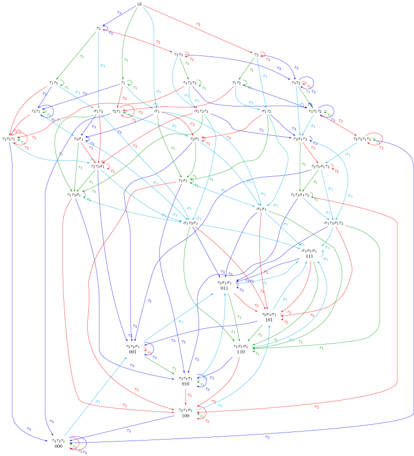
Figure 10. The left Cayley graph of the monoid for the one-dimensional Landslide sandpile model with three sites. The constant function subgraph agrees with Figure 8.

An element $e$ of a monoid $M$ is called idempotent if $e=e^{2}$. The set of idempotents of $M$ is denoted $E(M)$. If $M$ is finite, then each element $m$ has a unique idempotent positive power, traditionally written $m^{\omega}$. Let $X$ be a generating set for a monoid $M$. Then the content of an idempotent $e$ is defined to be the set $c(e)=\{x\in X\mid e\in MxM\}$. In other words, $x\in c(e)$ if and only if $e=mxm^{\prime}$ for some $m,m^{\prime}\in M$.

A monoid is ${\mathscr{R}}$-trivial if $aM=bM$ for $a,b\in M$ is equivalent to $a=b$. Similarly, a monoid is $\mathscr{J}$-trivial if $MaM=MbM$ for $a,b\in M$ is equivalent to $a=b$. If $M$ is $\mathscr{J}$-trivial, then it is well-known that $e=e^{\prime}$ if and only if $c(e)=c(e^{\prime})$ for $e,e^{\prime}\in E(M)$. See for instance Chapter 8 of [Alm94]. Also a monoid $M$ is ${\mathscr{R}}$-trivial if and only if, for each $e\in E(M)$, one has $ex=e$ for all $x\in c(e)$; see Theorem 5.1 of [BF80]. The classes of $\mathscr{J}$-trivial monoids and ${\mathscr{R}}$-trivial monoids are easily verified to be closed under taking submonoids.

Associated to an ${\mathscr{R}}$-trivial monoid is a lattice. The following can all be extracted from Chapter 8 of [Alm94] or Chapter 6 of [RS09], where things are considered in much greater generality. A more recent exposition, closer to our viewpoint, can be found in [MS12]. We say that two idempotents $e,f\in M$ are ${\mathscr{L}}$-equivalent if $ef=e$ and $fe=f$. The equivalence class of $e$ will be denoted by $[e]$. The set $\Lambda(M)$ of equivalence classes of idempotents is a lattice where the order is given by $[e]\leq[f]$ if and only if $ef=e$. The largest element of $\Lambda(M)$ is the class of the identity and the meet of two elements $e,f$ is $[(ef)^{\omega}]$.

The following theorem is a special case of the results of the third author [Ste06, Ste08].

Theorem 3.1.

Let $M$ be an ${\mathscr{R}}$-trivial monoid acting on a set $\Omega$. Let $\mathbb{P}$ be a probability distribution on $M$ and let $\mathcal{M}$ be the Markov chain with state set $\Omega$, where the transition probability from $x$ to $y$ is the probability that $mx=y$ (if $m$ is chosen according to $\mathbb{P}$). Then the transition matrix has an eigenvalue

$$\lambda_{[e]}=\sum_{[m^{\omega}]\geq[e]}\mathbb{P}(m)$$

for each $[e]\in\Lambda(M)$. The multiplicities $\boldsymbol{m}_{[e]}$, $[e]\in\Lambda(M)$, are determined recursively by the equation

$$|e\Omega|=\sum_{[f]\leq[e]}\boldsymbol{m}_{[f]}.$$

3.2. Wreath products

We refer to Eilenberg [Eil76] for the wreath product of left transformation monoids (except he uses right transformation monoids). Another reference is the book [Mel95a]. Let $[n]=\{0,\ldots,n\}$. If $M$ is a monoid acting faithfully on the left of $[n]$ and $N$ is a monoid acting faithfully on the left of $X$, then $(M,[n])\wr(N,X)$ is the monoid $W$ acting faithfully on $[n]\times X$ defined as follows. An element $f\in W$ is of the form

(3.1) $$f=\gamma_{f}(f_{0},\ldots,f_{n})\;,$$

where $\gamma_{f}\in M$ and $f_{i}\in N$, for $0\leq i\leq n$. The product is given by

$$\gamma_{f}(f_{0},\ldots,f_{n})\cdot\gamma_{g}(g_{0},\ldots,g_{n})=\gamma_{f}\gamma_{g}(f_{\gamma_{g}(0)}g_{0},\ldots,f_{\gamma_{g}(n)}g_{n}).$$

The action of $f$ as in (3.1) on $[n]\times X$ is given by $f(k,x)=(\gamma_{f}(k),f_{k}(x))$. If $\gamma_{f}$ is the identity, then we just write $f=(f_{0},\ldots,f_{n})$. The monoid $W$ will be denoted $M\wr N$ when the underlying sets $[n]$ and $X$ are clear.

An alternative representation of this wreath product is via column monomial matrices. A matrix is column monomial if each column contains exactly one non-zero entry. Let $\mathscr{T}_{n}$ denote the monoid of all self-maps of $[n]$. Then the wreath product $\mathscr{T}_{n}\wr N$ can be identified with the monoid of all column monomial $n\times n$ matrices over $N\cup\{0\}$ with the usual matrix multiplication. Notice addition is never needed when multiplying column monomial matrices. The matrix corresponding to an element $\gamma_{f}(f_{0},\ldots,f_{n})$ is the matrix where the unique non-zero entry of column $j$ is $f_{j}$ and this element is placed in row $\gamma_{f}(j)$. For example if $f=\gamma(f_{0},f_{1},f_{2})$ where (in two-line notation for a function)

$$\gamma=\begin{pmatrix}0&1&2\\ 0&0&2\end{pmatrix},$$

then the corresponding column monomial matrix is

$$f=\begin{bmatrix}f_{0}&f_{1}&0\\ 0&0&0\\ 0&0&f_{2}\end{bmatrix}.$$

If $M$ is a monoid acting on the left of a set $X$, then the associated linear representation $\rho_{X}\colon M\to M_{|X|}(\mathbb{C})$ is given by

$$\rho_{X}(m)_{ij}=\begin{cases}1&\text{if}\ mj=i,\\ 0&\text{else.}\end{cases}$$

Crucial to this paper is the following observation. Consider the Markov chain $\mathcal{M}$ with state space $X$ where if we are in state $x$, then we choose an element $m\in M$ with probability $p_{m}$ and we transition from $x$ to $mx$. Then the transition matrix of $\mathcal{M}$ is given by

$$\sum_{m\in M}p_{m}\cdot\rho_{X}(m).$$

This is why the representation theory of monoids is potentially useful to analyze Markov chains.

Let $\rho_{X}\colon N\to M_{|X|}(\mathbb{C})$ be the linear representation associated to the action of $N$ on $X$. To describe the linear representation $\rho\colon\mathscr{T}_{n}\wr N\to M_{n|X|}(\mathbb{C})$ associated to the action of $\mathscr{T}_{n}\wr N$ on $[n]\times X$, we should think of $\mathbb{C}^{n|X|}$ as $\mathbb{C}^{n}\otimes\mathbb{C}^{|X|}$. Then $\rho(f)$ is given by the block column monomial matrix obtained by applying $\rho_{X}$ to each entry of the column monomial matrix associated to $f$ (where $\rho_{X}(0)$ is understood to be the $|X|\times|X|$ zero matrix).

3.3. A wreath product approach to sandpile models

Let $\mathcal{T}=(V,E,T)$ be the data for the arborescence as in Section 2.1. Let $\Omega(\mathcal{T})$ be the state space of the Markov chain associated to $\mathcal{T}$ (see Eq. (2.1)). If $\ell\in L$ is a leaf, define $\nabla_{\ell}\mathcal{T}$ to consist of the arborescence obtained by removing the leaf $\ell$ from the vertex set $V$, the outgoing edge from $\ell$ from the edge set $E$, and $T_{\ell}$ from the threshold vector $T$. In this section we shall allow an empty arborescence. Note that $\Omega(\emptyset)$ is a one-element set.

If $w\in V$ is any vertex of our arborescence we can define an operator $\sigma_{w}$ on $\Omega(\mathcal{T})$ analogously to the way the source operator in Section 2.3 was defined for leaves. For the empty arborescence, we interpret $\sigma_{\emptyset}$ by convention to be the identity on $\Omega(\emptyset)$. We can define a successor operator on the vertices of an arborescence by letting $\mathop{\boldsymbol{s}}(v)$ be the endpoint of the unique edge from $v$. For convenience, set $\mathop{\boldsymbol{s}}({\mathsf{r}})=\emptyset$.

An important role is played in this paper by two families of monoids corresponding to the two variants of the sandpile model. The monoids associated to $\mathcal{T}$ are given by

$$N(\mathcal{T})=\langle\sigma_{v},\theta_{v}\mid v\in V\rangle\quad\text{and}\quad M(\mathcal{T})=\langle\sigma_{v},\tau_{v}\mid v\in V\rangle.$$

Note that $N(\emptyset)=M(\emptyset)=\{\sigma_{\emptyset}\}$. Also, since $\tau_{v}=\theta^{T_{v}}_{v}$, it follows that $M(\mathcal{T})$ is a submonoid of $N(\mathcal{T})$.

The monoids $N(\mathcal{T})$ and $M(\mathcal{T})$ can be described recursively as follows. Fix a leaf $\ell\in L$ of $\mathcal{T}$ and observe that $\Omega(\mathcal{T})=[T_{\ell}]\times\Omega(\nabla_{\ell}\mathcal{T})$. We then have the recursions in Table 1, where $t\in\Omega(\nabla_{\ell}\mathcal{T})$, $t_{\ell}\in[T_{\ell}]$, and the operators on the right hand side are viewed as mappings on $\Omega(\nabla_{v}\mathcal{T})$.

$$\sigma_{\ell}(t_{\ell},t) =\begin{cases}(t_{\ell}+1,t)&\text{if}\ t_{\ell}<T_{\ell}\\ (T_{\ell},\sigma_{\mathop{\boldsymbol{s}}(\ell)}t)&\text{if}\ t_{\ell}=T_{\ell}\end{cases}$$

$$\sigma_{v}(t_{\ell},t) =(t_{\ell},\sigma_{v}t) (v\neq\ell)$$

$$\theta_{\ell}(t_{\ell},t) =\begin{cases}(t_{\ell}-1,\sigma_{\mathop{\boldsymbol{s}}(\ell)}t)&\text{if}\ t_{\ell}>0\\ (0,t)&\text{if}\ t_{\ell}=0\end{cases}$$

$$\theta_{v}(t_{\ell},t) =(t_{\ell},\theta_{v}t) (v\neq\ell)$$

$$\tau_{\ell}(t_{\ell},t) =(0,\sigma_{\mathop{\boldsymbol{s}}(\ell)}^{t_{\ell}}t)$$

$$\tau_{v}(t_{\ell},t) =(t_{\ell},\tau_{v}t) (v\neq\ell).$$

Table 1. Recursions for sandpile operators

To rephrase the recursions in Table 1 in the language of wreath products, we need to introduce some notation. For an $m\geq 0$, define mappings $\alpha_{m}$ and $\beta_{m}$ on $[m]$ as follows:

$$\alpha_{m}(h) =\begin{cases}h+1&\text{if}\ h<m,\\ m&\text{if}\ h=m,\end{cases}$$

$$\beta_{m}(h) =\begin{cases}h-1&\text{if}\ h>0,\\ 0&\text{if}\ h=0.\end{cases}$$

Denote by $\overline{k}$ the constant mapping on $[m]$ with image $k$. Let $N(m)=\langle\alpha_{m},\beta_{m}\rangle$ and $M(m)=\langle\alpha_{m},\overline{0}\rangle$. Note that $M(m)\subseteq N(m)$.

Clearly

$$N(\mathcal{T}) \subseteq(N(T_{\ell}),[T_{\ell}])\wr(N(\nabla_{\ell}\mathcal{T}),\Omega(\nabla_{\ell}\mathcal{T}))\;,$$

$$M(\mathcal{T}) \subseteq(M(T_{\ell}),[T_{\ell}])\wr(M(\nabla_{\ell}\mathcal{T}),\Omega(\nabla_{\ell}\mathcal{T}))\;.$$

Indeed, we have

(3.2) $$\begin{split}\sigma_{\ell}&=\alpha_{T_{\ell}}(\varepsilon,\ldots,\varepsilon,\sigma_{\mathop{\boldsymbol{s}}(\ell)})\\ \sigma_{v}&=(\sigma_{v},\ldots,\sigma_{v})\qquad\qquad\qquad\qquad(v\neq\ell)\\ \theta_{\ell}&=\beta_{T_{\ell}}(\varepsilon,\sigma_{\mathop{\boldsymbol{s}}(\ell)},\sigma_{\mathop{\boldsymbol{s}}(\ell)},\ldots,\sigma_{\mathop{\boldsymbol{s}}(\ell)})\\ \theta_{v}&=(\theta_{v},\ldots,\theta_{v})\qquad\qquad\qquad\qquad(v\neq\ell)\\ \tau_{\ell}&=\overline{0}(\varepsilon,\sigma_{\mathop{\boldsymbol{s}}(\ell)},\sigma^{2}_{\mathop{\boldsymbol{s}}(\ell)},\ldots,\sigma^{T_{\ell}}_{\mathop{\boldsymbol{s}}(\ell)})\\ \tau_{v}&=(\tau_{v},\ldots,\tau_{v})\qquad\qquad\qquad\qquad(v\neq\ell).\end{split}$$

The wreath product setting immediately yields a convenient description of the action of the generators by multiplication on the right.

Remark 3.2.

Take $f:=\gamma_{f}(f_{0},\ldots,f_{T_{\ell}})\in M(\mathcal{T})$ and $m\in M(\nabla_{\ell}\mathcal{T})$. Then,

$$\begin{split}\gamma_{f}(f_{0},\ldots,f_{T_{\ell}})\ \tau_{\ell}&=\overline{\gamma_{f}(0)}(f_{0},f_{0}\sigma_{\ell},\ldots,f_{0}\sigma_{\mathop{\boldsymbol{s}}(\ell)}^{T_{\ell}})\,,\\ \gamma_{f}(f_{0},\ldots,f_{T_{\ell}})\ \sigma_{\ell}&=(\gamma_{f}\circ\alpha_{T_{\ell}})(f_{1},\ldots,f_{T_{\ell}+1})\,,\\ \gamma_{f}(f_{0},\ldots,f_{T_{\ell}})\ m&=\gamma_{f}(f_{0}m,\ldots,f_{T_{\ell}}m)\,,\end{split}$$

where, for notational convenience, $f_{i}:=f_{T_{\ell}}\sigma_{\mathop{\boldsymbol{s}}(\ell)}^{i-T_{\ell}}$ for $i>T_{\ell}$.

4. Stationary distributions

In this section we prove the stationary distributions stated in Section 2. In Section 4.1 we use a master equation approach to prove Theorem 2.3. Both Theorems 2.3 and 2.8 are proved in Section 4.2 using wreath products.

4.1. Master equation proof

We recall basic facts about the stationary distribution of a finite Markov chain. The stationary probability of every configuration $t\in\Omega$ satisfies the master equation

(4.1) $$\sum_{t^{\prime}\in\Omega}\text{probability}(t\to t^{\prime})\;\mathbb{P}(t)=\sum_{t^{\prime\prime}\in\Omega}\text{probability}(t^{\prime\prime}\to t)\;\mathbb{P}(t^{\prime\prime}),$$

namely that the total weight of the outgoing transitions of any configuration is equal to the incoming weight. In cases where the chain is ergodic, the solution to (4.1) is unique up to an overall scaling factor. This factor is determined by the fact that the sum of all probabilities is one. Let us denote by

$$\mathrm{Out}(t) =\{t^{\prime}\;|\;\text{probability}(t\to t^{\prime})\neq 0\}$$

$$\mathrm{In}(t) =\{t^{\prime\prime}\;|\;\text{probability}(t^{\prime\prime}\to t)\neq 0\}$$

the sets of outgoing and incoming configurations into $t$. For reversible Markov chains, $\mathrm{Out}(t)=\mathrm{In}(t)$ and this equation is satisfied term by term simply by setting $t^{\prime\prime}=t^{\prime}$. This is essentially the definition of a reversible chain.

For nonreversible Markov chains, this is not true. In special cases, the pairwise balance condition [SRB96] is satisfied which says that there is an invertible map $\phi\colon\mathrm{Out}(t)\to\mathrm{In}(t)$ so that for every $t^{\prime}\in\mathrm{Out}(t)$, $\phi(t)=t^{\prime\prime}$ satisfies

(4.2) $$\text{probability}(t\to t^{\prime})\;\mathbb{P}(t)=\text{probability}(t^{\prime\prime}\to t)\;\mathbb{P}(t^{\prime\prime}).$$

Obviously, a necessary condition for this to work is that $|\mathrm{Out}(t)|=|\mathrm{In}(t)|$ for all $t\in\Omega$.

We will need a variant of the pairwise balance condition, which we describe now. Suppose $P_{O}(t)$ (respectively $P_{I}(t)$) is a set partition of $\mathrm{Out}(t)$ (respectively $\mathrm{In}(t)$) of the same cardinality and further that there exists an invertible map $\Phi\colon P_{O}(t)\to P_{I}(t)$ which satisfies for every $\wp\in P_{O}$,

(4.3) $$\sum_{t^{\prime}\in\wp}\text{probability}(t\to t^{\prime})\;\mathbb{P}(t)=\sum_{t^{\prime\prime}\in\Phi(\wp)}\text{probability}(t^{\prime\prime}\to t)\;\mathbb{P}(t^{\prime\prime}).$$

If this happens for all $t$, then the master equation (4.1) holds and we say that partitioned balance holds.

Proof of Theorem 2.3.

By Proposition 2.2, this chain is ergodic, and hence has a unique stationary distribution. Therefore, we simply need to check that $\mathbb{P}(t)$ given by formula (2.4) satisfies the master equation (4.1) for a generic configuration $t\in\Omega$. Set $|V|=n$.

We will do so by showing that partitioned balance holds with $n+1$ partitions of $\mathrm{Out}(t)$. $n$ of these partitions correspond to singletons $\{\theta_{v}(t)\}$ for all $v\in V$. The last partition is given by the $\{\sigma_{\ell}(t)\mid\ell\in L\}$. Clearly, these form a set partition of $\mathrm{Out}(t)$.

We will first describe $\Phi(\{\theta_{v}(t)\})$ and show that (4.3) is satisfied. If $t_{v}=0$, then $\theta_{v}(t)=t$ and we set $\Phi(\{\theta_{v}(t)\})=\{t\}$. In this case (4.3) reduces to (4.2), which is easy to check.

When $t_{v}\neq 0$, we first describe the set $\Phi(\{\theta_{v}(t)\})$ in words. It is the set of all possible configurations $t^{\prime\prime}$ which make a transition to $t$ in such a way that the last grain falls at site $v$. Note that this can happen either by toppling another vertex or by entering at a leaf. More precisely, a branch is a contiguous set of all vertices in $\ell^{\downarrow}\setminus v^{\downarrow}$ for a given leaf $\ell\in L$, ending in $v$ but not including $v$, which are filled to the threshold in configuration $t$. Define $B_{t}(v)$ to be the set of all branches for any $\ell\in L$. Then $B_{t}(v)\cap L$ is the set of leaves of the filled branches, which are the branches where all the vertices from the leaf to $v$ are filled to the threshold. Similarly, let

$$W_{t}(v)=\{w\in\bigcup_{\ell\in L_{v}}(\ell^{\downarrow}\setminus v^{\downarrow})\setminus B_{t}(v)\mid\text{$w$ adjacent to $B_{t}(v)$}\}.$$

In other words, the set of vertices in $W_{t}(v)$ are those that sit just above an unfilled branch.

If $w\in W_{t}(v)$, define $t^{(v,w)}$ as follows. Let $t^{(v,w)}_{v}=t_{v}-1,t^{(v,w)}_{w}=t_{w}+1$ and $t^{(v,w)}_{u}=t_{u}$ for all other vertices $u$. For $\ell\in B_{t}(v)\cap L$, let $t^{(v,\ell)}$ be the configuration such that $t^{(v,\ell)}_{v}=t_{v}-1$ and $t^{(v,\ell)}_{u}=t_{u}$ for all other vertices $u$. Then

$$\Phi(\{\theta_{v}(t)\})=\{t^{(v,w)}\mid w\in W_{t}(v)\}\cup\{t^{(v,\ell)}\mid\ell\in B_{t}(v)\cap L\}\;.$$

To verify (4.3) for this partition, we have to show that

$$x_{v}\mathbb{P}(t)=\sum_{w\in W_{t}(v)}x_{w}\mathbb{P}(t^{(v,w)})+\sum_{\ell\in B_{t}(v)\cap L}y_{\ell}\mathbb{P}(t^{(v,\ell)})\;.$$

But, dividing by $\frac{x_{v}}{Y_{v}}\mathbb{P}(t)$ and using (2.4) for the probabilities, this amounts to showing

$$Y_{v}=\sum_{w\in W_{t}(v)}Y_{w}+\sum_{\ell\in B_{t}(v)\cap L}y_{\ell},$$

and this is easy to see from the definition of $Y_{v}=\sum_{\ell\in L_{v}}y_{\ell}$.

So far, we have considered all possible interior topplings in $\mathrm{Out}(t)$ and all possible transitions which end with a sand grain being deposited in the interior. We now consider the last partition of $\mathrm{Out}(t)$ given by the action of the boundary operators $\{\sigma_{\ell}(t)\mid\ell\in L\}$. We will show that the corresponding configurations in $\mathrm{In}(t)$ are those which end with a sand grain leaving from the root.

As before, we consider all branches of the root $\widetilde{B}_{t}({\mathsf{r}})$, this time including the root. Note that if the root is not filled to the threshold, only ${\mathsf{r}}$ belongs to this set. We use the same terminology as in the first half of the proof and let $\widetilde{W}_{t}({\mathsf{r}})\subseteq\bigcup_{\ell\in L}\ell^{\downarrow}\setminus\widetilde{B}_{t}({\mathsf{r}})$ denote the vertices which have an arrow to a vertex in $\widetilde{B}_{t}({\mathsf{r}})$. As before, for $w\in\widetilde{W}_{t}({\mathsf{r}})$ we define $t^{({\mathsf{r}},w)}$ to be the configurations with $t^{({\mathsf{r}},w)}_{{\mathsf{r}}}=t_{{\mathsf{r}}}-1$, and $t^{({\mathsf{r}},w)}_{u}=t_{u}$ for all other vertices $u$. For $\ell\in\widetilde{B}_{t}({\mathsf{r}})\cap L$, we define $t^{({\mathsf{r}},\ell)}=t$. The case $t^{({\mathsf{r}},\ell)}$ corresponds to the situation where a path from leaf $\ell$ to ${\mathsf{r}}$ is completely filled to the threshold in $t$. Thus, we have to show

$$\sum_{\ell\in L}y_{\ell}\mathbb{P}(t)=\sum_{w\in\widetilde{W}_{t}({\mathsf{r}})}x_{w}\mathbb{P}(t^{({\mathsf{r}},w)})+\sum_{\ell\in\widetilde{B}_{t}({\mathsf{r}})\cap L}y_{\ell}\mathbb{P}(t^{({\mathsf{r}},\ell)}).$$

Dividing by $\mathbb{P}(t)$ on both sides and using (2.4), we obtain

$$\sum_{\ell\in L}y_{\ell}=\sum_{w\in\widetilde{W}_{t}({\mathsf{r}})}Y_{w}+\sum_{\ell\in\widetilde{B}_{t}({\mathsf{r}})\cap L}y_{\ell},$$

and this is also true exactly as before. Therefore we have confirmed that pairwise balance holds for this model using the probabilities given by (2.4). This completes the proof. ∎

An alternative proof of Theorem 2.3 with an algebraic flavor is presented in Section 4.2.

4.2. Stationary distributions via wreath products

We now use the wreath product representation of Section 3.3 to give an alternative proof of Theorem 2.3 and a proof of Theorem 2.8. We use the notation of these theorems and of Section 3.2.

What we shall actually do is prove a more general result. Suppose that we have operators $\psi_{1},\ldots,\psi_{r}$ acting on a set $\Omega^{\prime}$ and a threshold $T$. Let $\Omega=[T]\times\Omega^{\prime}$. Set $N=\langle\psi_{1},\ldots,\psi_{r}\rangle$. We define elements in $(N(T),[T])\wr(N,\Omega^{\prime})$ as follows:

$$\sigma_{0} =\alpha_{T}(\varepsilon,\ldots,\varepsilon,\psi_{1})$$

$$\theta_{0} =\beta_{T}(\varepsilon,\psi_{1},\ldots,\psi_{1})$$

$$\Psi_{i} =\,\,\,\,\,\,\,(\psi_{i},\ldots,\psi_{i}) (1\leq i\leq r).$$

For example, the operators defining $N(\mathcal{T})$ for the Trickle-down sandpile model are of this form, as are the operators defining $M(\mathcal{T})$ for the Landslide sandpile model if $T_{\ell}=1$, where $\ell$ is the distinguished leaf considered above.

In column monomial form the above operators are given by

(4.4) $$\begin{split}\sigma_{0}&=\begin{bmatrix}0&0&\cdots&0&0\\ I&0&\ddots&0&0\\ 0&I&\ddots&0&\vdots\\ \vdots&0&\ddots&0&0\\ 0&0&\cdots&I&\psi_{1}\end{bmatrix},\qquad\theta_{0}=\begin{bmatrix}I&\psi_{1}&0&\cdots&\vdots\\ 0&0&\psi_{1}&0&0\\ \vdots&0&\ddots&\ddots&0\\ 0&0&\ddots&0&\psi_{1}\\ 0&0&\cdots&0&0\end{bmatrix},\\ \Psi_{i}&=\begin{bmatrix}\psi_{i}&0&\cdots&0\\ 0&\psi_{i}&\ddots&\vdots\\ \vdots&\ddots&\ddots&0\\ 0&\cdots&0&\psi_{i}\end{bmatrix}\qquad\qquad(1\leq i\leq r).\end{split}$$

where we are thinking of $\mathbb{C}^{|\Omega|}$ as $\mathbb{C}^{T}\otimes\mathbb{C}^{|\Omega^{\prime}|}$.

Consider the Markov chain $\mathcal{M}$ with state set $\Omega$, where $\sigma_{0}$ is applied with probability $y_{0}$, $\theta_{0}$ is applied with probability $x_{0}$, and $\Psi_{i}$ is applied with probability $z_{i}$. Let us also consider the derived Markov chain $\mathcal{M}^{\prime}$ with state set $\Omega^{\prime}$, where the $\psi_{i}$ are applied with probabilities

(4.5) $$z^{\prime}_{i}=\begin{cases}\dfrac{z_{1}+y_{0}}{1-x_{0}}&\text{if}\ i=1,\\ \dfrac{z_{i}}{1-x_{0}}&\text{if}\ 2\leq i\leq r.\end{cases}$$

Proposition 4.1.

Suppose that $\mathbb{P}^{\prime}$ is a stationary distribution for $\mathcal{M}^{\prime}$ and define

$$\pi(h)=\dfrac{y_{0}^{h}x_{0}^{T-h}}{\sum_{i=0}^{T}x_{0}^{i}y_{0}^{T-i}}.$$

Then the product measure $\mathbb{P}=\pi\times\mathbb{P}^{\prime}$ on $\Omega$ is a stationary distribution for $\mathcal{M}$, that is, $\mathbb{P}(h,t)=\pi(h)\mathbb{P}^{\prime}(t)$ for all $(h,t)\in\Omega$ is stationary for $\mathcal{M}$.

Proof.

Straightforward computation shows that $\pi$ is a probability distribution on $[0,T]$ and that

(4.6) $$\pi(h)=\left(\frac{y_{0}}{x_{0}}\right)\pi(h-1)\qquad(1\leq h\leq T).$$

Denote by $M$ the transition matrix of $\mathcal{M}$ and $M^{\prime}$ the transition matrix of $\mathcal{M}^{\prime}$. Then $M=y_{0}\sigma_{0}+x_{0}\theta_{0}+\sum_{i=1}^{r}z_{i}\Psi_{i}$ and $M^{\prime}=\sum_{i=1}^{r}z_{i}^{\prime}\psi_{i}$. It then follows from (4.4) that $M$ has the block tridiagonal form

$$M=\begin{bmatrix}x_{0}I+A&x_{0}\psi_{1}&&&0\\ y_{0}I&A&x_{0}\psi_{1}&\\ &\ddots&\ddots&\ddots&\\ &&y_{0}I&A&x_{0}\psi_{1}\\ 0&&&y_{0}I&y_{0}\psi_{1}+A\end{bmatrix}\;,$$

where

$$A=\sum_{i=1}^{r}z_{i}\psi_{i}=(1-x_{0})M^{\prime}-y_{0}\psi_{1}$$

by (4.5). In block vector form we have $\mathbb{P}=\left[\pi(0)\mathbb{P}^{\prime},\ldots,\pi(T)\mathbb{P}^{\prime}\right]^{T}$. We then compute by direct matrix multiplication the block form of $M\mathbb{P}$ using that $M^{\prime}\mathbb{P}^{\prime}=\mathbb{P}^{\prime}$ and repeated application of (4.6):

$$[M\mathbb{P}]_{0} =\pi(0)\left[x_{0}+(1-x_{0})M^{\prime}-y_{0}\psi_{1}\right]\mathbb{P}^{\prime}+\pi(1)x_{0}\psi_{1}\mathbb{P}^{\prime}$$

$$=\pi(0)\mathbb{P}^{\prime}+\left[\pi(1)x_{0}-\pi(0)y_{0}\right]\psi_{1}\mathbb{P}^{\prime}$$

$$=\pi(0)\mathbb{P}^{\prime};$$

$$[M\mathbb{P}]_{h} =\pi(h-1)y_{0}\mathbb{P}^{\prime}+\pi(h)\left[(1-x_{0})M^{\prime}-y_{0}\psi_{1}\right]\mathbb{P}^{\prime}+\pi(h+1)x_{0}\psi_{1}\mathbb{P}^{\prime}$$

$$=\left[\pi(h-1)y_{0}-\pi(h)x_{0}\right]\mathbb{P}^{\prime}+\pi(h)\mathbb{P}^{\prime}+\left[\pi(h+1)x_{0}-\pi(h)y_{0}\right]\psi\mathbb{P}^{\prime}$$

$$=\pi(h)\mathbb{P}^{\prime}\qquad\qquad(\text{for}\ 0<h<T);$$

$$[M\mathbb{P}]_{T} =\pi(T-1)y_{0}\mathbb{P}^{\prime}+\pi(T)(1-x_{0})M^{\prime}\mathbb{P}^{\prime}$$

$$=\pi(T)\mathbb{P}^{\prime}+\left[\pi(T-1)y_{0}-\pi(T)x_{0}\right]\mathbb{P}^{\prime}$$

$$=\pi(T)\mathbb{P}^{\prime}.$$

Therefore, $M\mathbb{P}=\mathbb{P}$ and so $\mathbb{P}$ is stationary. ∎

We can now deduce Theorem 2.3.

Proof of Theorem 2.3.

We retain the notation of Section 3.3. We work by induction on the number of vertices, the theorem being trivial for no vertices. Let $\mathcal{M}$ be the Markov chain with state space $\Omega(\mathcal{T})$ where $\sigma_{v}$ has probability $y_{v}$ for all $v\in V$ and $\theta_{v}$ has probability $x_{v}$ for all $v\in V$. Let

$$Y_{v}=\sum_{w\geq v}y_{w}.$$

Define $\rho_{v}$, for $v\in V$, and $\mathbb{P}$ as in (2.3) and (2.4), respectively (but with the above definition of $Y_{v}$). We prove $\mathbb{P}$ is the stationary distribution for $\mathcal{M}$. Theorem 2.3 will then follow by setting $y_{v}=0$ if $v$ is not a leaf.

Let $\mathcal{M}^{\prime}$ be the Markov chain with state space $\Omega(\nabla_{v}\mathcal{T})$ with probabilities

$$\widetilde{y}_{v}=\begin{cases}\dfrac{y_{\mathop{\boldsymbol{s}}(\ell)}+y_{\ell}}{1-x_{\ell}}&\text{if}\ v=\mathop{\boldsymbol{s}}(\ell),\\ \dfrac{y_{v}}{1-x_{\ell}}&\text{if}\ v\neq\mathop{\boldsymbol{s}}(\ell),\end{cases}$$

for the $\sigma_{v}$ and probabilities $\widetilde{x}_{v}=\frac{x_{v}}{1-x_{\ell}}$ for the $\theta_{v}$ with $v\in V\setminus\{\ell\}$. For $v\in V\setminus\{\ell\}$, let

$$\widetilde{Y}_{v}=\sum_{w\geq v}\widetilde{y}_{w}.$$

Using that $v<\ell$ if and only if $v\leq\mathop{\boldsymbol{s}}(\ell)$, we conclude that

(4.7) $$\widetilde{Y}_{v}=\frac{Y_{v}}{1-x_{\ell}}.$$

Denote by $\mathbb{P}^{\prime}$ the stationary distribution of $\mathcal{M}^{\prime}$. Notice that if

$$\rho^{\prime}_{v}(h)=\frac{\widetilde{Y}_{v}^{h}\;\widetilde{x}_{v}^{T_{v}-h}}{\sum_{i=0}^{T_{v}}\widetilde{Y}_{v}^{i}\;\widetilde{x}_{v}^{T_{v}-i}},$$

then $\rho^{\prime}_{v}(h)=\rho_{v}(h)$ by (4.7). By induction, we may assume that the stationary distribution $\mathbb{P}^{\prime}$ of $\mathcal{M}^{\prime}$ is given by

$$\mathbb{P}^{\prime}(t)=\prod_{v\in V\setminus\{\ell\}}\rho_{v}^{\prime}(v)=\prod_{v\in V\setminus\{\ell\}}\rho_{v}(v).$$

Proposition 4.1 now implies that

$$\mathbb{P}(t)=\prod_{v\in V}\rho_{v}(v),$$

as required. ∎

Next we prove Theorem 2.8.

Proof of Theorem 2.8.

Notice that if the threshold $T_{v}$ is $1$, then $\theta_{v}=\tau_{v}$. Therefore, the inductive step of the proof of Theorem 2.8 proceeds identically to that of the proof of Theorem 2.3. The difference is only in the base case, which will be when the graph just contains the root. In that case we just have state space $[T_{{\mathsf{r}}}]$ and with probability $y_{{\mathsf{r}}}$ we increase the number of grains by $1$ to a threshold of $T_{{\mathsf{r}}}$ and with probability $x_{{\mathsf{r}}}$ we go to $0$. This is precisely the classical winning streak Markov chain [LPW09, Example 4.15] and (2.5) is the well-known stationary distribution for that chain. ∎

5. ${\mathscr{R}}$-triviality, eigenvalues, and rate of convergence for the Landslide sandpile model

In this section we first show that the monoid associated to the Landslide sandpile model is ${\mathscr{R}}$-trivial. This is then used to prove the eigenvalues of the transition matrix of this model and the rate of convergence.

5.1. ${\mathscr{R}}$-triviality of $M(\mathcal{T})$

Let us again fix $\mathcal{T}$ an arborescence with a threshold vector. We retain the notation of Section 3.3. In particular, $\ell$ will denote a fixed leaf throughout this subsection.

Define a partial order, called the dominance order, on $\Omega(\mathcal{T})$ as follows: $t$ is dominated by $t^{\prime}$, written $t\unlhd t^{\prime}$, if for each vertex $v$ one has

$$\sum_{w\geq v}t_{w}\leq\sum_{w\geq v}t^{\prime}_{w}.$$

A mapping $f$ on $\Omega(\mathcal{T})$ is order-preserving if $f(t)\unlhd f(t^{\prime})$ whenever $t\unlhd t^{\prime}$. It is called decreasing if $f(t)\unlhd t$. The set of all order-preserving and decreasing mappings on a poset is well-known to be a ${\mathscr{J}}$-trivial monoid. See e.g. [Pin86] or [DHST11] for details.

Lemma 5.1.

The following hold.

1. The mappings $\{\tau_{v}\mid v\in V\}$ preserve the dominance order and are decreasing. Thus the monoid $J(\mathcal{T})=\langle\tau_{v}\mid v\in V\rangle$ is $\mathscr{J}$-trivial.

2. The mappings $\{\sigma_{v}\mid v\in V\}$ preserve the dominance order, commute and are increasing. Thus the commutative monoid $\langle\sigma_{v}\mid v\in V\rangle$ is $\mathscr{J}$-trivial.

3. All mappings in the monoid $M(\mathcal{T})$ preserve dominance order.

Proof.

We prove part (1) as the other parts are similar to, or a direct consequence of, part (1). Since by definition $\tau_{v}=\theta_{v}^{T_{v}}$, it suffices to prove that $\theta_{v}$ is decreasing and order preserving. Because $\theta_{v}$ moves at most one grain lower down in the arborescence, it is clear that it is a decreasing map. It remains to prove that it is order preserving. First we introduce some notation.

Recall that the $\zeta$-transform of $t\in\Omega$ (a vector indexed by $V$) is defined by $\zeta(t)_{v}=\sum_{w\geq v}t_{w}$ for a vertex $v$ and note that $t\unlhd t^{\prime}$ if and only if $\zeta(t)_{v}\leq\zeta(t^{\prime})_{v}$ for all vertices $v$. Suppose now that $t\unlhd t^{\prime}$. If $t^{\prime}_{v}=0$, then $\theta_{v}(t)\unlhd t\unlhd t^{\prime}=\theta_{v}(t^{\prime})$ and we are done. So assume that $t^{\prime}_{v}>0$.

Since $\theta_{v}$ changes a state only in vertices belonging to $v^{\downarrow}$, we have that if $w\nleq v$, then $\zeta(\theta_{v}(t))_{w}=\zeta(t)_{w}\leq\zeta(t^{\prime})_{w}=\zeta(\theta_{v}(t^{\prime}))_{w}$. Thus it suffices to prove $\zeta(\theta_{v}(t))_{w}\leq\zeta(\theta_{v}(t^{\prime}))_{w}$ if $w\leq v$.

Suppose $w=v$. If $t_{v}>0$, then clearly $\zeta(\theta_{v}(t))_{v}=\zeta(t)_{v}-1\leq\zeta(t^{\prime})_{v}-1=\zeta(\theta_{v}(t^{\prime}))_{v}$. On the other hand, if $t_{v}=0$, then $\theta_{v}(t)=t$ and so (recalling $t^{\prime}_{v}>0$)

$$\zeta(\theta_{v}(t))_{v}=\zeta(t)_{v}=\sum_{u\gtrdot v}\zeta(t)_{u}\leq\sum_{u\gtrdot v}\zeta(t^{\prime})_{u}\leq\zeta(t^{\prime})_{v}-1=\zeta(\theta_{v}(t^{\prime}))_{v}\;,$$

where $u\gtrdot v$ means $u$ covers $v$ in the ordering on vertices. Thus $\zeta(\theta_{v}(t))_{v}\leq\zeta(\theta_{v}(t^{\prime}))_{v}$ in either case.

Next suppose that $w<v$ and that $t^{\prime}_{u}=T_{u}$ for all $w\leq u<v$. Let $Y$ consist of those vertices $y\geq w$ such that $y$ is incomparable with $v$ and let $X$ be the set of minimal elements of $Y$. Note that each vertex of $Y$ is above a unique vertex of $X$ because we are in a tree. Also if $x\in X$, then $x\ngeq v$ and so $\zeta(\theta_{v}(t))_{x}=\zeta(t)_{x}\leq\zeta(t^{\prime})_{x}=\zeta(\theta_{v}(t^{\prime}))_{x}$. Then

$$\zeta(\theta_{v}(t))_{w} =\zeta(\theta_{v}(t))_{v}+\sum_{w\leq u<v}\theta_{v}(t)_{u}+\sum_{x\in X}\zeta(\theta_{v}(t))_{x}$$

$$\leq\zeta(\theta_{v}(t^{\prime}))_{v}+\sum_{w\leq u<v}T_{u}+\sum_{x\in X}\zeta(\theta_{v}(t^{\prime}))_{x}=\zeta(\theta_{v}(t^{\prime}))_{w}\;.$$

Finally, suppose that $w<v$ and that $t^{\prime}_{u}<T_{u}$ for some $u$ with $w\leq u<v$. Then since $\theta_{v}(t)\unlhd t$, we have

$$\zeta(\theta_{v}(t))_{w}\leq\zeta(t)_{w}\leq\zeta(t^{\prime})_{w}=\zeta(\theta_{v}(t^{\prime}))_{w}\;,$$

where the last equality follows because the grain of sand that was toppled from $v$ winds up at some vertex $v^{\prime}$ with $w\leq v^{\prime}<v$. This completes the proof that $\theta_{v}$ (and hence $\tau_{v}$) is order preserving. ∎

In order to simultaneously handle a mix between topple and source operators, we will need to split, according to the circumstances, the tree $\mathcal{T}$ into a downset and an upset, and to control the action of the operators on these two parts in a different fashion.

For an idempotent $e$, define

(5.1) $$L(e):=\bigcup_{\{v\in V\mid\sigma_{v}\in c(e)\}}v^{\downarrow}$$

and $U(e):=L(e)^{c}$ (where $X^{c}$ is the complement of a set $X$). Note that $L(e)$ is a downset and $U(e)$ is an upset.

On an upset the control comes from order preserving properties. Namely, for an upset $U\subseteq V$, define the dominance preorder $\unlhd_{U}$ on $\Omega(\mathcal{T})$ analogously to the usual dominance order except we only take into account vertices in $U$; that is, $t\unlhd_{U}t^{\prime}$ if, for all $v\in U$, we have

$$\sum_{w\geq v}t_{w}\leq\sum_{w\geq v}t^{\prime}_{w}.$$

We write $t\equiv_{U}t^{\prime}$ if $t\unlhd_{U}t^{\prime}$ and $t^{\prime}\unlhd_{U}t$, that is, if $t$ and $t^{\prime}$ coincide on $U$. As with the full dominance order, the monoid $M(\mathcal{T})$ interacts nicely with this preorder. The fact that $\equiv_{U}$ is compatible with the action of $M(\mathcal{T})$ means that $M(\mathcal{T})$ embeds in the generalized wreath product indexed by a poset as discussed in [Mel95b].

Lemma 5.2.

Let $U$ be an upset of $V$ in $\mathcal{T}$.

1. The mappings $\{\tau_{v}\mid v\in V\}$ preserve the dominance preorder $\unlhd_{U}$ and are decreasing.

2. The mappings $\{\sigma_{v}\mid v\in V\}$ preserve the dominance preorder $\unlhd_{U}$ and are increasing.

3. Furthermore, if $v\not\in U$, then $\sigma_{v}t\equiv_{U}t$ and $\tau_{v}t\equiv_{U}t$ for all $t\in\Omega(\mathcal{T})$.

On a downset, control comes from the fact that functions involving repeated source operators tend to be constant below these sources. This is best expressed in the wreath product setting and we start with some general remarks, whose proofs are straightforward.

Proposition 5.3.

Suppose that $f=\gamma_{f}(f_{0},\ldots,f_{T_{\ell}})\in M(\mathcal{T})$. Then $f$ is an idempotent if and only if $\gamma_{f}=\varepsilon$ and $f_{i}^{2}=f_{i}$ for all $0\leq i\leq T_{\ell}$ or $\gamma_{f}=\overline{k}$ and $f_{k}f_{i}=f_{i}$, for $0\leq i\leq T_{\ell}$ (and so in particular $f_{k}^{2}=f_{k}$).

Proof.

If $f$ is an idempotent, then $\gamma_{f}$ must be an idempotent, and hence by definition of $M(T_{\ell})$ either $\gamma_{f}=\varepsilon$ or $\gamma_{f}=\overline{k}$ for some $0\leq k\leq T_{\ell}$. In the first case, we have

$$f^{2}=(f_{0},\ldots,f_{T_{\ell}})^{2}=(f_{0}^{2},\ldots,f_{T_{\ell}}^{2})$$

and hence $f$ is idempotent if and only if $f_{i}^{2}=f_{i}$ for $0\leq i\leq T_{\ell}$. In the second case, we have

$$f^{2}=\overline{k}(f_{0},\ldots,f_{T_{\ell}})\overline{k}(f_{0},\ldots,f_{T_{\ell}})=\overline{k}(f_{k}f_{0},\ldots,f_{k}f_{T_{\ell}})$$

and so $f$ is idempotent if and only if $f_{k}f_{i}=f_{i}$ for all $0\leq i\leq T_{\ell}$. ∎

We say that $m\in M(\mathcal{T})$ is constant with value $k_{v}\in[T_{v}]$ at the vertex $v$ if $(mt)_{v}=k_{v}$ for all $t\in\Omega(\mathcal{T})$.

Remark 5.4.

If $m\in M(\mathcal{T})$ is constant at the vertex $v$ with value $k_{v}$, then so is $mm^{\prime}$ for all $m^{\prime}\in M(\mathcal{T})$. This follows, because putting $t^{\prime}=m^{\prime}t$, we have $(mm^{\prime}t)_{v}=(mt^{\prime})_{v}=k_{v}$.

It will be convenient to describe the property of being constant at a vertex in terms of wreath product coordinates. Recall that $\ell\in L$ is the chosen fixed leaf.

Remark 5.5.

Let $m=\gamma_{m}(m_{0},\ldots,m_{T_{\ell}})\in M(\mathcal{T})$. Then $m$ is constant at $\ell$ with value $k_{\ell}$ if and only if $\gamma_{m}=\overline{k}_{\ell}$. If $v\neq\ell$, then $m$ is constant with value $k_{v}$ at $v$ if and only if each $m_{t_{\ell}}$, with $0\leq t_{\ell}\leq T_{\ell}$, is constant with value $k_{v}$ at $v$. This is immediate because $m(t_{\ell},t)=(\gamma_{m}(t_{\ell}),m_{t_{\ell}}t)$.

For the next statement we need the notion of words representing monoid elements. Let $f\in M(\mathcal{T})$. Then an expression $f=g_{1}\cdots g_{r}$ in terms of the generators $g_{i}\in\{\sigma_{v},\tau_{v}\mid v\in V\}$ is called a word representing $f$. If $w$ is a word in the generators of $M(\mathcal{T})$, the corresponding element of $M(\mathcal{T})$ will be written in wreath product coordinates as $\gamma_{w}(w_{0},\ldots,w_{T_{\ell}})$.

Proposition 5.6.

If $w$ is a word with at least $r$ occurrences of $\sigma_{\ell}$ with $\ell\in L$, then each $w_{i}$ is represented by a word with at least $r+i-T_{\ell}$ occurrences of $\sigma_{\mathop{\boldsymbol{s}}(\ell)}$.

Proof.

We proceed by induction on the length of the word $w$. If $w$ is empty, there is nothing to prove. Assume that the proposition holds for a word $u$ and that $w=ug$ with $g$ a generator. Suppose that $u$ has at least $r$ occurrences of $\sigma_{\ell}$. Then we have three cases. If $g=\tau_{\ell}$, then by Remark 3.2 we have $w_{i}=u_{0}\sigma_{\mathop{\boldsymbol{s}}(\ell)}^{i}$ and so $w_{i}$ is represented by a word with at least $r+i-T_{\ell}$ occurrences of $\sigma_{\mathop{\boldsymbol{s}}(\ell)}$ by induction. If $g=\sigma_{\ell}$, then Remark 3.2 shows that $w_{i}=u_{i+1}$, where $u_{T_{\ell}+1}=u_{T_{\ell}}\sigma_{\mathop{\boldsymbol{s}}(\ell)}$. Thus by induction $w_{i}$ has at least $r+i+1-T_{\ell}=r+1+i-T_{\ell}$ occurrences of $\sigma_{\mathop{\boldsymbol{s}}(\ell)}$. Finally, if $g\neq\tau_{\ell},\sigma_{\ell}$, then $w_{i}=u_{i}g$ and the result follows by induction. ∎

The following technical lemma is the key statement for proving that $M(\mathcal{T})$ is $\mathscr{R}$-trivial.

Lemma 5.7.

Let $e\in E(M(\mathcal{T}))$ and let $\sigma_{v}\in c(e)$. Then $e$ is constant at each $w\in v^{\downarrow}$.

Proof.

The proof proceeds by induction on the number of vertices in the arborescence. The statement is vacuous when there are no vertices. Let us write $e=\gamma_{e}(e_{0},\ldots,e_{T_{\ell}})$. We distinguish two cases: $v\neq\ell$ and $v=\ell$.

Case 1: $v\neq\ell$. Let $w\leq v$. By Proposition 5.3, either $\gamma_{e}=\varepsilon$ or $\gamma_{e}=\overline{k}$ for some $0\leq k\leq T_{\ell}$. When $\gamma_{e}=\varepsilon$, $e_{i}^{2}=e_{i}$ for all $i$. Also, neither $\sigma_{\ell}$, nor $\tau_{\ell}$ can belong to $c(e)$. A glance at (3.2) then shows that $e_{0}=\cdots=e_{T_{\ell}}=e^{\prime}$ for some $e^{\prime}\in E(M(\nabla_{\ell}\mathcal{T}))$ with $c(e^{\prime})=c(e)$. Thus, by induction, $e^{\prime}$ is constant at $w$. But then $e$ is constant at $w$ by Remark 5.5.

Next suppose that $\gamma_{e}=\overline{k}$ with $0\leq k\leq T_{\ell}$. Then $e_{k}^{2}=e_{k}$ and $e_{k}e_{i}=e_{i}$ for $0\leq i\leq T_{\ell}$. According to Remark 5.5, in order for $e$ to be constant at $v$ with value $k_{v}$, we need each $e_{i}$ to be constant at $v$ with value $k_{v}$. In light of Remark 5.4 and the equalities $e_{k}e_{i}=e_{i}$, it suffices to show that $e_{k}$ is constant at $v$ with value $k_{v}$. By induction, it therefore is enough to show that $\sigma_{v}\in c(e_{k})$. This follows immediately from Remark 3.2 with $m=\sigma_{v}$.

Case 2: $v=\ell$. Let $w\leq\ell$. Note that $\gamma_{e}=\overline{k}$ for some $0\leq k\leq T_{\ell}$ because $\sigma_{\ell}\in c(e)$. Hence $e_{k}^{2}=e_{k}$ and $e_{k}e_{i}=e_{i}$ for all $0\leq i\leq T_{\ell}$.

If $w=\ell$, then we are done by Remark 5.5, so assume $w<\ell$. Since $e$ is idempotent and $\sigma_{\ell}\in c(e)$, we can represent $e$ by a word with at least $T_{\ell}+1$ occurrences of $\sigma_{\ell}$. Proposition 5.6 then yields $\sigma_{\mathop{\boldsymbol{s}}(\ell)}\in c(e_{k})$. Then by induction $e_{k}$ is constant at $w$. Arguing as in the previous case, we conclude that $e$ is constant at $w$. ∎

An immediate corollary is the following crucial fact.

Corollary 5.8.

If $e\in E(M(\mathcal{T}))$, then $e$ is constant at each $w\in L(e)$.

We are now in position to state and prove the main theorem of this section.

Theorem 5.9.

The monoid $M(\mathcal{T})$ is ${\mathscr{R}}$-trivial.

Proof.

As noted in Section 3.1, it is sufficient to take any idempotent $e\in E(M(\mathcal{T}))$ and $g\in c(e)$ and prove that $eg=e$. We will do that by controlling $e$ separately on $L(e)$ and its complement $U(e)$. Take $t\in\Omega(\mathcal{T})$. By Corollary 5.8 $e$ is constant on $L(e)$ and so $egt$ and $et$ coincide on $L(e)$ (cf. Remark 5.4). Thus, it just remains to prove that $egt$ and $et$ also coincide on $U(e)$, that is, $egt\equiv_{U(e)}et$. First note that by the definition of $L(e)$, if $\sigma_{v}\in c(e)$, then $v\notin U(e)$.

Case 1: $g$ is of the form $\sigma_{v}$ or $\tau_{v}$ with $v\notin U(e)$. Lemma 5.2 then yields $gt\equiv_{U(e)}t$, and therefore $et\equiv_{U(e)}et$.

Case 2: $g$ is of the form $\tau_{v}$ with $v\in U(e)$. Here we use the same trick as in the usual proof of ${\mathscr{J}}$-triviality of a decreasing order-preserving monoid of transformations. Namely, using that $\tau_{v}\in c(e)$, write $e=h\tau_{v}h^{\prime}$. Note that any expression of $h$ and $h^{\prime}$ as a product of generators contains no $\sigma_{u}$ with $u\in U(e)$ by the definition of $c(e)$ and $L(e)$ (5.1). This implies by Lemma 5.2 that $h,h^{\prime},\tau_{v}$ preserve $\unlhd_{U(e)}$ and are decreasing on $U(e)$. Therefore, we can conclude with:

$$et=e^{2}t=eh\tau_{v}h^{\prime}t\unlhd_{U(e)}e\tau_{v}t\unlhd_{U(e)}et\,.\qed$$

5.2. Eigenvalues

Our goal is to compute the eigenvalues for the Landslide sandpile model using Theorem 3.1. To each $S\subseteq V$, we associate an idempotent

(5.2) $$e_{S}:=\left(\prod_{v\in S}\tau_{v}\right)^{\omega}.$$

Since $J(\mathcal{T})$ is $\mathscr{J}$-trivial, the resulting idempotent is independent of the order in which the product is taken. Note that $e_{\emptyset}$ is the identity, whereas $e_{V}$ sends all of $\Omega(\mathcal{T})$ to the zero vector.

The reader should recall the definition of the lattice associated to an ${\mathscr{R}}$-trivial monoid in Section 3.1. Note that $S_{1}\subseteq S_{2}$ if and only if $e_{S_{2}}e_{S_{1}}=e_{S_{2}}$, if and only if $[e_{S_{1}}]\geq[e_{S_{1}}]$. Thus the lattice $\Lambda(J(\mathcal{T}))$ associated to $J(\mathcal{T})$ is isomorphic to the lattice of subsets of $V$ ordered by reverse inclusion.

Proposition 5.10.

The lattice $\Lambda(M(\mathcal{T}))$ of idempotents of $M(\mathcal{T})$ coincides with that of $J(\mathcal{T})$.

This is an immediate consequence of the following lemma.

Lemma 5.11.

Let $e$ be an idempotent of $M(\mathcal{T})$, and define

$$S(e)=L(e)\cup\{v\mid\tau_{v}\in c(e)\}\,.$$

Then $e$ is ${\mathscr{L}}$-equivalent to the idempotent $e_{S(e)}$ of $J(\mathcal{T})$.

Proof.

Suppose that $v\in U(e)$. Then we have that $\sigma_{v}\notin c(e)$ by definition of $L(e)$ and that $\tau_{v}\in c(e)$ if and only if $\tau_{v}\in c(e_{S(e)})$. Thus $et\equiv_{U(e)}e_{S(e)}t$ for all $t\in\Omega$ by Lemma 5.2 (consider a word $w$ representing $e$ containing each $\tau_{v}\in c(e)$ and raise it to a large power; then use the third item of Lemma 5.2). Another application of Lemma 5.2 then yields

$$e_{S(e)}et\equiv_{U(e)}e_{S(e)}^{2}t=e_{S(e)}t\equiv_{U(e)}et=e^{2}t\equiv_{U(e)}ee_{S(e)}t.$$

It thus remains to show that $ee_{S(e)}t$ and $et$ (respectively, $e_{S(e)}et$ and $e_{S(e)}t$) coincide on $L(e)$. To do this, it suffices by Remark 5.4 to verify that $e$ and $e_{S(e)}$ are both constant at each vertex of $L(e)$. For $e$, this is the precisely the conclusion of Corollary 5.8. We claim that $e_{S(e)}$ is constant with value $0$ at each vertex of $L(e)$. Indeed, since $e_{S(e)}$ belongs to the ${\mathscr{J}}$-trivial monoid $\langle\tau_{v}\mid v\in V\rangle$, we have that $\tau_{v}e_{S(e)}=e_{S(e)}$ for all $v\in L(e)$. As $\tau_{v}$ is constant with value $0$ at $v$, we conclude that $e_{S(e)}$ is constant with value $0$ at all vertices of $L(e)$ (cf. Remark 5.4). ∎

We now have all the ingredients to describe the eigenvalues of the Landslide sandpile model. This is achieved by computing the character of $M(\mathcal{T})$ acting on $\Omega(\mathcal{T})$ – which boils down to counting fixed points of idempotents – and inverting that data using the character table – which reduces to Möbius inversion along $\Lambda(M(\mathcal{T}))$ (i.e. inclusion-exclusion).

Proof of Theorem 2.10.

Observe that the fixed point set of $e_{S}$ is

$$e_{S}\Omega=\{t\in\Omega\mid t_{v}=0\ \text{for all}\ v\in S\}\,.$$

For $S\subseteq V$, write $S^{c}$ for $V\setminus S$. Set

$$\Upsilon_{S}:=\{t\in\Omega\mid t_{v}=0\iff v\in S\}\,.$$

Note that $|\Upsilon_{S}|=\prod_{v\in S^{c}}T_{v}=T_{S^{c}}$. Also we have that

(5.3) $$e_{S}\Omega=\biguplus_{X\supseteq S}\Upsilon_{X}\,.$$

Recall that $\Lambda(M(\mathcal{T}))$ is isomorphic to the lattice of subsets of $V$ ordered by reverse inclusion via the mapping $[e_{S}]\mapsto S$. If $\ell$ is a leaf, then $S(\sigma_{\ell}^{\omega})=\ell^{\downarrow}$. Thus $[\sigma_{\ell}^{\omega}]\geq[e_{S}]$ if and only if $\ell^{\downarrow}\subseteq S$. On the other hand, $[\tau_{v}]\geq[e_{S}]$ if and only if $v\in S$. It then follows from Theorem 3.1 that to each subset $S\subseteq V$ there is an associated eigenvalue $\lambda_{S}=x_{S}+y_{S}$, where $x_{S}$ and $y_{S}$ are defined in (2.6).

Let $\boldsymbol{m}_{S}$ be the multiplicity of $\lambda_{S}$. As $[e_{S}]\in\Lambda(M(\mathcal{T}))$ corresponds to the subset $S$, Theorem 3.1 implies

$$|e_{S}\Omega|=\sum_{X\supseteq S}\boldsymbol{m}_{X}.$$

By (5.3) we have

$$|e_{S}\Omega|=\sum_{X\supseteq S}|\Upsilon_{X}|=\sum_{X\supseteq S}T_{X^{c}}$$

and so Möbius inversion (see for example [Sta99]) yields $\boldsymbol{m}_{S}=T_{S^{c}}$ for all $S\subseteq V$, as desired. ∎

5.3. Rate of convergence

In this section we prove Theorem 2.11. There is a general technique, called coupling from the past, which allows one to bound the distance to stationarity for an ergodic random walk coming from a monoid action. Roughly speaking, it says the following. Suppose that we have a random mapping representation of an ergodic Markov chain $\mathcal{M}$ with state set $\Omega$ coming from a probability distribution $\mathbb{P}$ on a monoid $M$ acting on $\Omega$. Assume furthermore that $M$ contains a constant map. Then the distance to stationarity after $k$ steps of $\mathcal{M}$ is bounded by the probability of not being at a constant map after $k$ steps of the right random walk on $M$ driven by $\mathbb{P}$. More precisely, we have the following reformulation of [BD98, Theorem 3].

Theorem 5.12.

Let $M$ be a monoid acting on a set $\Omega$ and let $\mathbb{P}$ be a probability distribution on $M$. Let $\mathcal{M}$ be the Markov chain with state set $\Omega$ such that the transition probability from $x$ to $y$ is the probability that $mx=y$ if $m$ is chosen according to $\mathbb{P}$. Assume that $\mathcal{M}$ is ergodic with stationary distribution $\pi$ and that some element of $M$ acts as a constant map on $\Omega$.

Letting $P^{k}$ be the distribution of $\mathcal{M}$ after $k$ steps and $\mathbb{P}^{k}$ be the $k^{th}$-convolution power of $\mathbb{P}$, we have that

$$\ \|P^{k}-\pi\|\leq\mathbb{P}^{k}(M\setminus C)\;,$$

where $C$ is the set of elements of $M$ acting as constants on $\Omega$.

In the context of the Landslide sandpile model we let $M$ be the submonoid of $M(\mathcal{T})$ generated by $\sigma_{v}$ with $v\in L$ and $\tau_{v}$ with $v\in V$. We shall define a statistic $u$ on $M$ so that $u(m)=0$ if and only if $m$ is a constant map. It follows from Theorem 5.12 that $\|P^{k}-\pi\|$ is bounded by the probability $u(m)>0$.

Proof of Theorem 2.11.

Let $m\in M$. Say that an upset $U$ of vertices is deterministic for $m$ if $mt=mt^{\prime}$ whenever $t\equiv_{U}t^{\prime}$ for $t,t^{\prime}\in\Omega$. Notice that the set $V$ of all vertices is deterministic for $m$. Also, if $U_{1},U_{2}$ are deterministic for $m$ and $U_{1}\cap U_{2}=U$, then $U$ is also deterministic for $m$. Indeed, if $t\equiv_{U}t^{\prime}$, choose $t^{\prime\prime}\in\Omega$ such that $t\equiv_{U_{1}}t^{\prime\prime}\equiv_{U_{2}}t^{\prime}$. This can be done because $t$ and $t^{\prime}$ agree on $U=U_{1}\cap U_{2}$. Then $mt=mt^{\prime\prime}=mt^{\prime}$. It follows that there exists a unique minimum deterministic upset $U(m)$ for $m$. Moreover, $m$ is constant on $\Omega$ if and only if $U(m)=\emptyset$. Define the statistic $u$ on $M$ by $u(m)=|U(m)|$. Then we have $0\leq u(m)\leq n$ where $n=|V|$, and $u(m)=0$ if and only if $m$ is constant. Note that $u(\varepsilon)=n$.

Claim 1: $u$ decreases along $\mathscr{R}$-order: $u(mm^{\prime})\leq u(m)$ for any $m,m^{\prime}\in M$. To see this, it suffices to show that $U(m)$ is deterministic for $mm^{\prime}$, whence $U(mm^{\prime})\subseteq U(m)$. If $t\equiv_{U(m)}t^{\prime}$ then by Lemma 5.2, $m^{\prime}t\equiv_{U(m)}m^{\prime}t$ and therefore $mm^{\prime}t=mm^{\prime}t^{\prime}$.

Claim 2: Assume that $v$ is a minimal element of $U(m)$. Then $u(m\tau_{v})<u(m)$. It suffices to show that $U^{\prime}=U(m)\setminus\{v\}$ is deterministic for $m\tau_{v}$. If $t\equiv_{U^{\prime}}t^{\prime}$, then $\tau_{v}t\equiv_{U^{\prime}}\tau_{v}t^{\prime}$ and furthermore $(\tau_{v}t)_{v}=0=(\tau_{v}t^{\prime})_{v}$. Therefore, $\tau_{v}t\equiv_{U(m)}\tau_{v}t^{\prime}$ and hence $m\tau_{v}(t)=m\tau_{v}(t^{\prime})$.

Let us call a step $m_{i}\mapsto m_{i+1}$ in the random walk on the right Cayley graph of $M$ successful if either $m_{i}$ is constant or $u(m_{i+1})<u(m_{i})$. Claim 1 implies that $u(m_{i})=u(m_{i+1})$ if the step is not successful. Thus the probability that $u(m)>0$ after $k$ steps of the right random walk on $M$ is the probability of having at most $n-1$ successful steps in the first $k$ steps.

Claim 2 says that each step has probability at least $p_{x}$ to be successful. Therefore, the probability that $u(m)>0$ after $k$ steps of the right random walk on $M$ is bounded above by the probability of having at most $n-1$ successes in $k$ Bernoulli trials with success probability $p_{x}$.

Using Chernoff’s inequality for the cumulative distribution function of a binomial random variable we obtain that (see for example [DL01, After Theorem 2.1])

$$||P^{k}-\pi||\leq\sum_{i=0}^{n-1}{k\choose i}p_{x}^{i}(1-p_{x})^{k-i}\leq\exp\left(-\frac{(kp_{x}-(n-1))^{2}}{2kp_{x}}\right)\,,$$

where the last inequality holds as long as $k\geq(n-1)/p_{x}$. ∎

References

- [AKS14] Arvind Ayyer, Steven Klee, and Anne Schilling. Combinatorial Markov chains on linear extensions. J. Algebraic Combin., 39(4):853–881, 2014.
- [Alm94] Jorge Almeida. Finite semigroups and universal algebra, volume 3 of Series in Algebra. World Scientific Publishing Co. Inc., River Edge, NJ, 1994. Translated from the 1992 Portuguese original and revised by the author.
- [AS10] Arvind Ayyer and Volker Strehl. The spectrum of an asymmetric annihilation process. In 22nd International Conference on Formal Power Series and Algebraic Combinatorics (FPSAC 2010), Discrete Math. Theor. Comput. Sci. Proc., AN, pages 461–472. Assoc. Discrete Math. Theor. Comput. Sci., Nancy, 2010.
- [AS13] Arvind Ayyer and Volker Strehl. Stationary distribution and eigenvalues for a de Bruijn process. In Ilias S. Kotsireas and Eugene V. Zima, editors, Advances in Combinatorics, pages 101–120. Springer Berlin Heidelberg, 2013.
- [ASST14] Arvind Ayyer, Anne Schilling, Benjamin Steinberg, and Nicolas M. Thiéry. -trivial monoids and Markov chains. International Journal of Algebra and Computation, to appear, 2014. (arXiv.1401.4250).
- [Ayy11] Arvind Ayyer. Algebraic properties of a disordered asymmetric Glauber model. Journal of Statistical Mechanics: Theory and Experiment, 2011(02):P02034, 2011.
- [BD98] Kenneth S. Brown and Persi Diaconis. Random walks and hyperplane arrangements. Ann. Probab., 26(4):1813–1854, 1998.
- [BF80] J. A. Brzozowski and Faith E. Fich. Languages of -trivial monoids. J. Comput. System Sci., 20(1):32–49, 1980.
- [BHR99] Pat Bidigare, Phil Hanlon, and Dan Rockmore. A combinatorial description of the spectrum for the Tsetlin library and its generalization to hyperplane arrangements. Duke Math. J., 99(1):135–174, 1999.
- [Big99] Norman L Biggs. Chip-firing and the critical group of a graph. Journal of Algebraic Combinatorics, 9(1):25–45, 1999.
- [Bjö08] Anders Björner. Random walks, arrangements, cell complexes, greedoids, and self-organizing libraries. In Building bridges, volume 19 of Bolyai Soc. Math. Stud., pages 165–203. Springer, Berlin, 2008.
- [Bjö09] Anders Björner. Note: Random-to-front shuffles on trees. Electron. Commun. Probab., 14:36–41, 2009.
- [BLS91] Anders Björner, László Lovász, and Peter W Shor. Chip-firing games on graphs. European J. Combin, 12(4):283–291, 1991.
- [Bro00] Kenneth S. Brown. Semigroups, rings, and Markov chains. J. Theoret. Probab., 13(3):871–938, 2000.
- [BTW87] Per Bak, Chao Tang, and Kurt Wiesenfeld. Self-organized criticality: An explanation of the 1/f noise. Physical Review Letters, 59(4):381–384, 1987.
- [CG12] Fan Chung and Ron Graham. Edge flipping in graphs. Adv. in Appl. Math., 48(1):37–63, 2012.
- [CLB03] Robert Cori and Yvan Le Borgne. The sand-pile model and Tutte polynomials. Advances in Applied Mathematics, 30(1):44–52, 2003.
- [CP61] A. H. Clifford and G. B. Preston. The algebraic theory of semigroups. Vol. I. Mathematical Surveys, No. 7. American Mathematical Society, Providence, R.I., 1961.
- [DEHP93] B. Derrida, M. R. Evans, V. Hakim, and V. Pasquier. Exact solution of a D asymmetric exclusion model using a matrix formulation. J. Phys. A, 26(7):1493–1517, 1993.
- [Deo74] Narsingh Deo. Graph theory with applications to engineering and computer science. Prentice-Hall Inc., Englewood Cliffs, N.J., 1974. Prentice-Hall Series in Automatic Computation.
- [Dha90] D. Dhar. Self-organized critical state of sandpile automaton models. Physical Review Letters, 64(14):1613–1616, 1990.
- [Dha99a] D. Dhar. The abelian sandpile and related models. Physica A: Statistical Mechanics and its Applications, 263(1):4–25, 1999.
- [Dha99b] Deepak Dhar. Some results and a conjecture for Manna’s stochastic sandpile model. Physica A: Statistical Mechanics and its Applications, 270(1):69–81, 1999.
- [Dha06] Deepak Dhar. Theoretical studies of self-organized criticality. Physica A: Statistical Mechanics and its Applications, 369(1):29 – 70, 2006. Fundamental Problems in Statistical Physics Proceedings of the 11th International Summerschool on ’Fundamental problems in statistical physics’, September 4–17, 2005, Leuven, Belgium 11th International Summerschool on ’Fundamental problems in statistical physics’.
- [DHST11] Tom Denton, Florent Hivert, Anne Schilling, and Nicolas M. Thiéry. On the representation theory of finite -trivial monoids. Sém. Lothar. Combin., 64:Art. B64d, 44, 2010/11.
- [Dia88] Persi Diaconis. Group representations in probability and statistics. Institute of Mathematical Statistics Lecture Notes—Monograph Series, 11. Institute of Mathematical Statistics, Hayward, CA, 1988.
- [Dia98] Persi Diaconis. From shuffling cards to walking around the building: an introduction to modern Markov chain theory. In Proceedings of the International Congress of Mathematicians, Vol. I (Berlin, 1998), number Extra Vol. I, pages 187–204, 1998.
- [DL01] L. Devroye and G. Lugosi. Combinatorial methods in density estimation. Springer Series in Statistics Series. Springer-Verlag, 2001.
- [Eil76] Samuel Eilenberg. Automata, languages, and machines. Vol. B. Academic Press [Harcourt Brace Jovanovich Publishers], New York, 1976. With two chapters (“Depth decomposition theorem” and “Complexity of semigroups and morphisms”) by Bret Tilson, Pure and Applied Mathematics, Vol. 59.
- [GMP02] Eric Goles, Michel Morvan, and Ha Duong Phan. The structure of a linear chip firing game and related models. Theoret. Comput. Sci., 270(1-2):827–841, 2002.
- [GNS00] R. I. Grigorchuk, V. V. Nekrashevich, and V. I. Sushchanskiĭ. Automata, dynamical systems, and groups. Tr. Mat. Inst. Steklova, 231(Din. Sist., Avtom. i Beskon. Gruppy):134–214, 2000.
- [GŻ01] Rostislav I. Grigorchuk and Andrzej Żuk. The lamplighter group as a group generated by a 2-state automaton, and its spectrum. Geom. Dedicata, 87(1-3):209–244, 2001.
- [Hig92] Peter M. Higgins. Techniques of semigroup theory. Oxford Science Publications. The Clarendon Press Oxford University Press, New York, 1992. With a foreword by G. B. Preston.
- [HLM+08] Alexander E Holroyd, Lionel Levine, Karola Mészáros, Yuyal Peres, James Propp, and David B Wilson. Chip-firing and rotor-routing on directed graphs. In and Out of Equilibrium 2, pages 331–364, 2008.
- [How95] John M. Howie. Fundamentals of semigroup theory, volume 12 of London Mathematical Society Monographs. New Series. The Clarendon Press Oxford University Press, New York, 1995. Oxford Science Publications.
- [IP98] E.V. Ivashkevich and V.B. Priezzhev. Introduction to the sandpile model. Physica A: Statistical Mechanics and its Applications, 254(1-2):97 – 116, 1998.
- [KRT68] K. Krohn, J. Rhodes, and B. Tilson. Algebraic theory of machines, languages, and semigroups. Edited by Michael A. Arbib. With a major contribution by Kenneth Krohn and John L. Rhodes. Academic Press, New York, 1968. Chapters 1, 5–9.
- [KSS06] Mark Kambites, Pedro V. Silva, and Benjamin Steinberg. The spectra of lamplighter groups and Cayley machines. Geom. Dedicata, 120:193–227, 2006.
- [LPW09] David A. Levin, Yuval Peres, and Elizabeth L. Wilmer. Markov chains and mixing times. American Mathematical Society, Providence, RI, 2009. With a chapter by James G. Propp and David B. Wilson.
- [Man91] S S Manna. Two-state model of self-organized criticality. Journal of Physics A: Mathematical and General, 24(7):L363, 1991.
- [Mel95a] J. D. P. Meldrum. Wreath products of groups and semigroups, volume 74 of Pitman Monographs and Surveys in Pure and Applied Mathematics. Longman, Harlow, 1995.
- [Mel95b] J. D. P. Meldrum. Wreath products of groups and semigroups, volume 74 of Pitman Monographs and Surveys in Pure and Applied Mathematics. Longman, Harlow, 1995.
- [MG69] Carolyn T. MacDonald and Julian H. Gibbs. Concerning the kinetics of polypeptide synthesis on polyribosomes. Biopolymers, 7(5):707–725, 1969.
- [MGP68] Carolyn T. MacDonald, Julian H. Gibbs, and Allen C. Pipkin. Kinetics of biopolymerization on nucleic acid templates. Biopolymers, 6(1):1–25, 1968.
- [MS12] Stuart Margolis and Benjamin Steinberg. Quivers of monoids with basic algebras. Compos. Math., 148(5):1516–1560, 2012.
- [Nek05] Volodymyr Nekrashevych. Self-similar groups, volume 117 of Mathematical Surveys and Monographs. American Mathematical Society, Providence, RI, 2005.
- [Pin86] J.-E. Pin. Varieties of formal languages. Foundations of Computer Science. Plenum Publishing Corp., New York, 1986. With a preface by M.-P. Schützenberger, Translated from the French by A. Howie.
- [PS04] Alexander Postnikov and Boris Shapiro. Trees, parking functions, syzygies, and deformations of monomial ideals. Trans. Amer. Math. Soc., 356(8):3109–3142 (electronic), 2004.
- [RS09] John Rhodes and Benjamin Steinberg. The -theory of finite semigroups. Springer Monographs in Mathematics. Springer, New York, 2009.
- [S+13] W. A. Stein et al. Sage Mathematics Software (Version 5.9). The Sage Development Team, 2013. http://www.sagemath.org.
- [SCc08] The Sage-Combinat community. Sage-Combinat: enhancing Sage as a toolbox for computer exploration in algebraic combinatorics, 2008. http://combinat.sagemath.org.
- [SD09] Tridib Sadhu and Deepak Dhar. Steady state of stochastic sandpile models. Journal of Statistical Physics, 134(3):427–441, 2009.
- [SRB96] Gunter M Schütz, Ramakrishna Ramaswamy, and Mustansir Barma. Pairwise balance and invariant measures for generalized exclusion processes. Journal of Physics A: Mathematical and General, 29(4):837, 1996.
- [Sta99] Richard P. Stanley. Enumerative combinatorics. Vol. 2, volume 62 of Cambridge Studies in Advanced Mathematics. Cambridge University Press, Cambridge, 1999. With a foreword by Gian-Carlo Rota and appendix 1 by Sergey Fomin.
- [Ste06] Benjamin Steinberg. Möbius functions and semigroup representation theory. J. Combin. Theory Ser. A, 113(5):866–881, 2006.
- [Ste08] Benjamin Steinberg. Möbius functions and semigroup representation theory. II. Character formulas and multiplicities. Adv. Math., 217(4):1521–1557, 2008.
- [SW98] Tomohiro Sasamoto and Miki Wadati. Exact results for one-dimensional totally asymmetric diffusion models. Journal of Physics A: Mathematical and General, 31(28):6057, 1998.
- [TB97] Goutam Tripathy and Mustansir Barma. Steady state and dynamics of driven diffusive systems with quenched disorder. Phys. Rev. Lett., 78:3039–3042, Apr 1997.
- [Tou05] Evelin Christiana Toumpakari. On the Abelian Sandpile Model. PhD thesis, University of Chicago, Department of Mathematics, 2005.