Exotic quantum holonomy and non-Hermitian degeneracies
in two-body Lieb-Liniger model

Abstract

An interplay of an exotic quantum holonomy and exceptional points is examined in one-dimensional Bose systems. The eigenenergy anholonomy, in which Hermitian adiabatic cycle induces nontrivial change in eigenenergies, can be interpreted as a manifestation of eigenenergy’s Riemann surface structure, where the branch points are identified as the exceptional points which are degeneracy points in the complexified parameter space. It is also shown that the exceptional points are the divergent points of the non-Abelian gauge connection for the gauge theoretical formulation of the eigenspace anholonomy. This helps us to evaluate anti-path-ordered exponentials of the gauge connection to obtain gauge covariant quantities.

I Introduction

A variation of a classical external parameter of a quantum system offers a way to manipulate quantum states. Almost since the dawn of the quantum theory, it has been recognized that the slow variation of the parameter ensures the adiabatic time evolution, where the quantum state can be pinned to an eigenspace of system’s Hamiltonian Born-ZP-51-165 ; Kato-JPSJ-5-435 . Later, the concept of quantum holonomy has been developed for adiabatic cycles on quantum systems. Among them, the phase holonomy, where an adiabatic cycle induces a nontrivial change in the phase of a quantum state LonguetHiggins-PRSL-344-147 ; Mead-JCP-70-2284 ; Berry-PRSLA-392-45 ; Wilczek-PRL-52-2111 , is a textbook result nowadays Bohm-GPQS-2003 . Recently, the quantum holonomy of exotic kind has been recognized in that an adiabatic cycle can induce changes both in the eigenvalue and the eigenspace of a stationary state Cheon-PLA-248-285 . Such changes are also referred to as eigenenergy and eigenspace anholonomies Tanaka-PRL-98-160407 .

Spectral degeneracies are crucial for the quantum holonomy. The phase holonomy is associated with a spectral degeneracy point, where a structure mathematically identical to the magnetic monopole resides, in the parameter space Berry-PRSLA-392-45 . As for the exotic quantum holonomy, it is shown, for a quantum kicked spin-$\frac{1}{2}$, that degenerate points in the complexified parameter space play the central role Kim-PLA-374-1958 . Such a non-Hermitian degeneracy point is known as an exceptional point KatoExceptionalPoint ; Heiss-JMP-32-3003 ; Heiss-CzecJP-54-1091 . There have been considerable number of recent works on exceptional points in non-Hermitian quantum physics phhqp ; Heiss-CzecJP-54-1091 ; biorthogonal .

It is natural to expect that the exceptional points govern the exotic quantum holonomy in general, once we accept the view that the anholonomies in eigenenergy and eigenspace are a manifestation of multiple-valuedness of the solution of the eigenvalue problem in the parameter space. We remind the readers that an eigenvalue equation of a Hamiltonian can be cast into an algebraic equation. Hence its multiple-valued solutions form a family, and the family coalesces at a branch point in the parameter space Heiss-JMP-32-3003 . The encirclement of the branch point induces the permutation of the eigenvalues and eigenspaces in the family, which is to be identified as the complex-analytic origin of the exotic quantum holonomy. This, however, is rather unexpected scenario, because the exceptional points emerge only when the Hamiltonian is far from Hermitian, in spite of the fact that the exotic quantum holonomy is induced by an adiabatic Hermitian cycle. Hence the question is whether a family of Hermitian Hamiltonians that define an adiabatic cycle really “encloses” exceptional points.

The aim of this manuscript is to offer another example of successful “exceptional point picture” for the exotic quantum holonomy, in quantum many-body systems. We examine the Lieb-Liniger model, which describes Bose particles confined in a one-dimensional space subject to the periodic boundary condition Lieb-PR-130-15 . Ushveridze showed that a non-Hermitian extension of this model has an infinite number of exceptional points Ushveridze-JPA-21-955 . Recently, it is shown that the Lieb-Liniger model exhibits the eigenenergy and eigenspace anholonomies Yonezawa-up-20130 . Hence, our purpose is to explain how the non-Hermitian degeneracies of this model and the exotic quantum holonomy that occurs in Hermitian Hamiltonian is interrelated. We here focus on the simplest case where the number of particles is two. We believe that the present two-body study offers the foundation for the case of an arbitrary number of particles.

The outline of this manuscript is the following. We introduce the Lieb-Liniger model in Section II. We also explain that an adiabatic Hermitian cycle of this model induces the exotic quantum anholonomy Yonezawa-up-20130 . We cover a non-Hermitian extension of the Lieb-Liniger model Duerr-PRA-79-023614 in Section III. We outline the analytic continuation of the quasi-momentum in Section IV. We show an association of the eigenenergy anholonomy with exceptional points in Section V. We explain the role of the exceptional points in the gauge theoretical formulation of eigenspace anholonomy in Section VI. We discuss the present result in Section VII. We summarize this manuscript in Section VIII.

II Quantum holonomy in Hermitian Lieb-Liniger model

We review the two-body Lieb-Liniger model Lieb-PR-130-15 and its exotic quantum holonomy Yonezawa-up-20130 . Throughout this manuscript, we examine the system that consists of two identical Bose particles confined within a one-dimensional space, which is $2\pi$-periodic. We assume that the two particles have a contact interaction whose strength is $g$. The system is described by the Hamiltonian:

$$H(g)=-\frac{1}{2}\left(\frac{\partial{}^{2}}{\partial x_{1}^{2}}+\frac{\partial{}^{2}}{\partial x_{2}^{2}}\right)+{g}\delta(x_{1}-x_{2}),$$ (1)

where the units are chosen such that $\hbar$ and the mass of a Bose particle are $1$.

We explain the standard method to solve the eigenvalue problem of $H(g)$ Lieb-PR-130-15 . We employ the Bethe ansatz, where an eigenfunction is expressed by two plane waves that are associated with quasi-momentum (rapidity) $k_{j}$ ($j=1,2$). The total momentum $\bar{k}\equiv k_{1}+k_{2}$ must be an integer, because the periodic boundary condition is imposed. On the other hand, the difference in the quasi-momenta $k\equiv k_{2}-k_{1}$ satisfies the condition that

$$J(g,k)\equiv k+\frac{2}{\pi}\arctan\frac{k}{g},$$ (2)

is an integer Lieb-PR-130-15 . Throughout this paper, $\arctan$ denotes the principal value of the inverse tangent. For odd $J(g,k)$, $k$ satisfies

$$k/g=\cot(\pi k/2),$$ (3)

whereas even $J(g,k)$ implies

$$k/g=-\tan(\pi k/2).$$ (4)

We call (3) and (4) the Bethe equations.

We look for the solution of the Bethe equations for real $g$. Let $k_{n}(g)$ denote the solution that satisfies $k_{n}(0)=n$, and smoothly depends on $g$ in the real axis $-\infty<g<\infty$. It suffices to examine the case where $n$ is a non-negative integer. $k_{n}(g)$ is either real or pure imaginary. The latter case describes the “clustering” of two particles, which occurs only when $n=0$ and $g<0$, or, $n=1$ and $g<-2/\pi$. We here summarize the relevant facts on $k_{n}(g)$ shown in Ref. Lieb-PR-130-15 : (a) $k_{n}(\infty)=n+1$, and accordingly $J(k_{n}(g),g)=n+1$ for $g>0$; (b) For $n>1$, $k_{n}(-\infty)=n-1$ and accordingly $J(k_{n}(g),g)=n-1$ for $g<0$; (c) $k_{0}(g)$ and $k_{1}(g)$ satisfy (3) and (4), respectively.

There remain freedoms to choose the signs of $\Im k_{n}(-\infty)$ for $n=0$ and $1$. Here we carry out the analytic continuation of $k_{n}(g)$ through the lower half plane of $g$ from $g>0$. Although this choice is arbitrary for our purpose, the present choice is consistent with the condition that the non-Hermitian Lieb-Liniger model describes the (forward-)time evolution correctly (see, Sec. III). As a result, we obtain $k_{n}(-\infty)=-i\infty$ for $n=0$ and $1$.

The eigenstates of the two-body Lieb-Liniger model are specified by two quantum numbers $\bar{k}$ and $n$, which must be both even or odd. The corresponding eigenenergy is

$$E_{\bar{k},n}(g)=\frac{1}{2}\left({\bar{k}}^{2}+\left\{k_{n}(g)\right\}^{2}\right).$$ (5)

We introduce a cycle $\mathcal{C}(g_{0})$ in real $g$-space to investigate the exotic quantum holonomy. The initial point of $\mathcal{C}(g_{0})$ is $g_{0}$. We increase $g$ adiabatically during $g_{0}\leq g<\infty$. Then, $g$ is suddenly flipped from $\infty$ to $-\infty$. Such a sudden flip has been investigated both in theory Olshanii-PRL-81-938 and experiments Haller-Science-325-1224 ; Haller-PRL-104-153203 to approach super Tonks-Girardeau gas. To finish $\mathcal{C}(g_{0})$, $g$ is adiabatically increased from $-\infty$ to $g_{0}$.

The exotic quantum holonomy is found in the two-body Lieb-Liniger model along the cycle $\mathcal{C}(g_{0})$ Yonezawa-up-20130 . We initialize the interaction strength as $g=g_{0}$, and prepare the system to be in the eigenstate specified by quantum numbers $(\bar{k},n)$. As we increase $g$ adiabatically, the energy of the system follows $E_{\bar{k},n}(g)$, which increases monotonically. When we arrive $g=\infty$, we assume that we suddenly switch the value of $g$ from $\infty$ to $-\infty$, keeping the system remain unchanged. Because of $E_{\bar{k},n}(\infty)=E_{\bar{k},n+2}(-\infty)$, the system is in the $(\bar{k},n+2)$ state after the switch. As we increase $g$ from $-\infty$ to $g_{0}$ adiabatically, the energy of the whole system arrives at $E_{\bar{k},n+2}(g_{0})$, which does not agree with the initial energy. This is the eigenenergy anholonomy of the two-body Lieb-Liniger model. Because the Hamiltonian is Hermitian for real $g$, the eigenenergy anholonomy implies the eigenspace anholonomy, i.e., the initial and final state vectors correspond to different eigenenergies and are thus orthogonal.

III Non-Hermitian Lieb-Liniger model

We shall show, in the following sections, that the spectral degeneracies that are hidden in the complexified parameter space governs the exotic quantum holonomy of the two-body Lieb-Liniger model. To carry out this, we introduce the complexification of the coupling strength $g$. We outline formal aspects of the consequence of the complexification in this section, and the details of the analytic continuations of relevant quantities will be explained in the following sections. We refer Ref. biorthogonal for the theory of non-Hermitian eigenvalue problem.

Here we focus on the lower-half plane of $g$. This is just a matter of convention in our analysis since there is a symmetry about the real axis in the complex $g$-plane. However, the present choice is suitable once we realize that the complexified Lieb-Liniger model describes the dissipative effect. In Ref. Duerr-PRA-79-023614 , it is shown that the presence of inelastic collisions implies that the imaginary part of the effective one-dimensional coupling constant must be zero or negative, i.e., $\Im(g)\leq 0$.

First of all, the complexification makes the Lieb-Liniger Hamiltonian $H(g)$  (1) non-Hermitian. An immediate consequence is that the two eigenvalue problems for $H(g)$ and $\left[{H}(g)\right]^{\dagger}$ become different because of the relation $\left[{H}(g)\right]^{\dagger}=H(g^{*})$. An eigenvalue of $\left[{H}(g)\right]^{\dagger}$ is given by $\left[E_{\bar{k},n}(g)\right]^{*}$, which may not be identical to $E_{\bar{k},n}(g)$.

From the comparison of the spectrum sets of ${H}(g)$ and $\left[{H}(g)\right]^{\dagger}$, there is a unique pair $(n^{\prime},n)$ that satisfies

$$\left\{E_{\bar{k},n^{\prime}}(g^{*})\right\}^{*}=E_{\bar{k},n}(g),$$ (6)

where we assume that ${H}(g)$ has no spectral degeneracy within the subspace specified by the total momentum $\bar{k}$. This assumption holds in the vicinity of the real axis. We note that the correspondence between $n^{\prime}$ and $n$ generally depends on the details of the analytic continuation and the value of $g$. We ignore the case $n^{\prime}\neq n$ because we focus on the neighborhood of the real axis of $g$, and assume $\left\{E_{\bar{k},n}(g^{*})\right\}^{*}=E_{\bar{k},n}(g)$. This implies

$$\left\{k_{n}(g^{*})\right\}^{*}=sk_{n}(g),$$ (7)

where $s$ is either $1$ or $-1$, depending on how the analytic continuation of $k_{n}(g)$ is carried out. Also, $s$ may depend on $n$ and $g$.

Eigenfunctions of $H(g)$ can be obtained through a standard way with the help of the Bethe ansatz. We refer Ref. Lieb-PR-130-15 for details. Let $\psi_{\bar{k},n}(x_{1},x_{2})$ be an eigenfunction that corresponds to the eigenenergy $E_{\bar{k},n}(g)$. Because of the Bose statistics, we will write down only the expressions of eigenfunctions in the region $R_{1}\equiv\left\{(x_{1},x_{2})|0\leq x_{1}\leq x_{2}\leq L\right\}$:

$$\psi_{\bar{k},n}(x_{1},x_{2};g)=\Phi_{\bar{k}}\left(\frac{x_{1}+x_{2}}{2}\right)\Psi_{n}(x_{2}-x_{1};g),$$ (8)

where

$$\Phi_{\bar{k}}(X) \equiv \frac{1}{\sqrt{2\pi}}e^{i\bar{k}X},$$ (9)

$$\Psi_{n}(x;g) = \begin{cases}\frac{1}{\sqrt{2\pi}}a^{(\mathrm{g})}(k)\cos\left[k(x-\pi)/2\right]&\text{for even $n$, }\\ \frac{1}{\sqrt{2\pi}}a^{(\mathrm{e})}(k)\sin\left[k(x-\pi)/2\right]&\text{for odd $n$, }\\ \end{cases}$$ (10)

and the following abbreviation is introduced:

$$k\equiv k_{n}(g).$$ (11)

Here we choose the normalization constants $a^{(\mathrm{g})}(k)$ and $a^{(\mathrm{e})}(k)$ being independent of $n$ in order to ensure that the eigenfunctions are continuous with respect to $g$.

We turn to $\psi^{\mathrm{L}}_{\bar{k},n}(x_{1},x_{2};g)$ that is an eigenfunction of $\left[{H}(g)\right]^{\dagger}$ corresponding to the eigenvalue $\left\{E_{\bar{k},n}(g)\right\}^{*}$. Because of $\left[{H}(g)\right]^{\dagger}={H}(g^{*})$, we find

$$\psi^{\mathrm{L}}_{\bar{k},n}(x_{1},x_{2};g)=\Phi_{\bar{k}}\left(\frac{x_{1}+x_{2}}{2}\right)\Psi^{\mathrm{L}}_{n}(x_{2}-x_{1};g),$$ (12)

where

$$\Psi^{\mathrm{L}}_{n}(x;g)=\begin{cases}\frac{1}{\sqrt{2\pi}}a^{\mathrm{L}(\mathrm{g})}(\tilde{k})\cos\left[\tilde{k}(x-\pi)/2\right]&\text{for even $n$, }\\ \frac{1}{\sqrt{2\pi}}a^{\mathrm{L}(\mathrm{e})}(\tilde{k})\sin\left[\tilde{k}(x-\pi)/2\right]&\text{for odd $n$, }\\ \end{cases}$$ (13)

and we introduce another abbreviation

$$\tilde{k}\equiv k_{n}(g^{*}).$$ (14)

We choose the following normalization condition

$$\langle{}\psi^{\mathrm{L}}_{\bar{k}^{\prime},n^{\prime}}(g){}|{}\psi_{\bar{k},n}(g){}\rangle=\delta_{\bar{k}^{\prime},\bar{k}}\delta_{n^{\prime},n}.$$ (15)

This implies

$$\left\{a^{\mathrm{L}(\mathrm{g})}(\tilde{k})\right\}^{*}a^{(\mathrm{g})}(k) = 2\left(1+\frac{\sin(\pi k)}{\pi k}\right)^{-1},$$ (16)

$$\left\{a^{\mathrm{L}(\mathrm{e})}(\tilde{k})\right\}^{*}a^{(\mathrm{e})}(k) = 2s\left(1-\frac{\sin(\pi k)}{\pi k}\right)^{-1},$$ (17)

where $s$ was introduced in (7).

IV Quasi-momentum Riemann surface

The exotic quantum holonomy in Lieb-Liniger model can be cast into the anholonomy of the quasi-momentum $k_{n}(g)$. As explained in Sec. II, the cycle $\mathcal{C}(g_{0})$ changes $k_{n}(g_{0})$ into $k_{n+2}(g_{0})$. We here examine the analytic continuation of $k_{n}(g)$ to provide the basis of the analysis in the following sections.

The quasi-momenta $k_{n}(g)$’s in the complex $g$-plane form Riemann surfaces. There are two kinds of Riemann surfaces that correspond to $k_{n}(g)$’s with even and odd $n$s, respectively, of the two-body Lieb-Liniger model. We first look at the Riemann surface that involves $k_{n}(g)$’s with even $n$.

We carry out the analytic continuation of $k_{n}(g)$. When $g$ is positive and $\epsilon$ is sufficiently small, $J(g+\epsilon,k_{n}(g+\epsilon))=n+1$ holds. Expanding this equation with respect to the small parameter $\epsilon$, we obtain

$$k_{n}(g+\epsilon)=k_{n}(g)+\epsilon G(g,k_{n}(g))+\mathcal{O}(\epsilon^{2}),$$ (18)

where

$$G(g,k)\equiv-\frac{\partial_{g}J(g,k)}{\partial_{k}J(g,k)}.$$ (19)

(18) is applicable to negative $g$ and arbitrary $n$. Note that (18) makes sense only when the denominator of $G(g,k)$ is non-zero. As long as we can find a way to avoid the breakdown of this condition, (18) provides a way to obtain $k_{n}(g)$ with an arbitrary $g$.

We examine the condition that the procedure above is inapplicable. We assume that $(g,k_{n}(g))$ satisfies $\partial_{k}J(g,k)=0$. This implies that $g$ is a branch point of $k_{n}(g)$. Indeed, we obtain

$$k_{n}(g+\epsilon)=k_{n}(g)\pm\sqrt{\epsilon G^{(2)}(g,k_{n}(g))}+\mathcal{O}(\epsilon),$$ (20)

where

$$G^{(2)}(g,k)\equiv-\frac{2\partial_{g}J(g,k)}{\partial_{k}^{2}J(g,k)},$$ (21)

as long as the denominator of $G^{(2)}(g,k)$ is nonzero. When $\partial_{k}^{2}J(g,k)$ vanishes, the branch point is of third or higher order. For the two-body Lieb-Liniger model, the degree of all branch points is two, as is to be seen below.

We enumerate the branch points by solving the equation $\partial_{k}J(g,k)=0$ under the condition that $J(g,k)$ is an integer. This is equivalent to

$$k=\pm\sqrt{-g(g+2/\pi)}$$ (22)

as long as $|g|<\infty$ holds.

In the real axis, the family $k_{n}(g)$’s with even $n$ has only one branch point at $g=0$, where two quasi-momenta $k_{0}(g)$ and $-k_{0}(g)$ degenerate and the other quasi-momenta are not involved. Accordingly the real branch point does not involve any spectral degeneracy.

Complex branch points of quasi-momenta, which are obtained numerically, are depicted in Figure 1. All the complex branch points are confined in the region $\Re\;g<0$. These complex branch points involve spectral degeneracies, because two quasi-momenta that are degenerate at a complex branch point provide different eigenenergies, except at the branch point. This leads to a coalescence of the eigenspaces. Such complex branch points are called Kato’s exceptional points KatoExceptionalPoint ; Heiss-JMP-32-3003 ; Heiss-CzecJP-54-1091 .

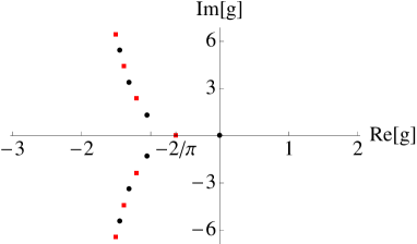
Figure 1: (Color online) Branch points of $k_{n}(g)$ in complex $g$-plane. Circles and squares correspond to even and odd $n$, respectively. When $n$ is even, we numerically obtain $g$ that simultaneously satisfies (22) and (3). There is only a single branch point $g=0$ on the real axis. All other complex branch points are in the region $\Re\;g<0$. We obtain the branch points for the odd $n$ case by solving (22) and (4). There is only a single branch point $g=-2/\pi$ on the real axis. All other complex branch points are in the region $\Re\;g<-2/\pi$.

Our numerical result is consistent with the argument above in the sense that all complex branch points are of degree two. We find that a complex branch point always involves $k_{0}(g)$, the quasi-momentum of the ground state. As far as we see, there is no branch point that involves two “excited states” $k_{n}(g)$ and $k_{n^{\prime}}(g)$ with $n,n^{\prime}>1$ at the same time. Also, each $k_{n}(g)$ with $n>1$ is involved with a complex branch point, which is denoted by $g^{(n)}$. Namely, $k_{0}(g)$ and $k_{n}(g)$ degenerate at $(g,k)=(g^{(n)},k^{(n)})$, where $k^{(n)}\equiv k_{0}(g^{(n)})=k_{n}(g^{(n)})$.

The numerical result can be explained qualitatively by a perturbation expansion around $g=-\infty$ Ushveridze-JPA-21-955 . The quasi-momentum of the ground state diverges as $k_{0}(g)\sim ig$ at $g\sim-\infty$ Lieb-PR-130-15 , where we ignore the small $g^{-1}$ correction. On the other hand, the quasi-momentum of the $n$-th excite state ($n>1$) converges to a constant value, i.e., $k_{n}(g)\sim n-1$ at $g\sim-\infty$ Lieb-PR-130-15 . Hence $k_{0}(g)$ and $k_{n}(g)$ coincides at $g\sim-i(n-1)$, which is considered to be an approximation of $g^{(n)}$ in the lower half-plane. Although this argument is consistent only when $n$ is large enough, the present estimation seems to be applicable to smaller $n$’s (see figure 1). We also remark that the configuration of exceptional points in the upper half-plane is due to the other branch of $k_{0}(g)$, i.e., $k_{0}(g)\sim-ig$ at $g\sim-\infty$.

We construct a Riemann sheet $k_{n}(g)$ in the complex plane as follows. For real numbers $g^{\prime}$ and $g^{\prime\prime}$, $k_{n}(g^{\prime}+ig^{\prime\prime})$ is extended from $k_{n}(g^{\prime})$ along the line parallel to the imaginary axis, if there is no branch point in the interval between $g^{\prime}$ and $g^{\prime}+ig^{\prime\prime}$. Branch cuts are chosen to be parallel to the imaginary axis. We also require that the branch cuts do not traverse the real axis. When there is a branch point in the real axis, the corresponding branch cut is located in the upper half plane. We depict some of the Riemann sheets in Fig 2.

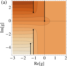
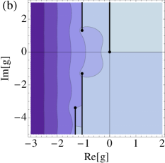
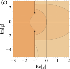
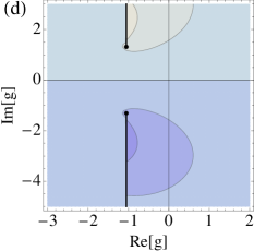
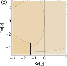
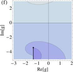
Figure 2: The Riemann sheets $k_{n}(g)$: (1st row) $n=0$; (2nd row) $n=2$; (3rd row) $n=4$. The real and imaginary parts are shown in the left and right columns, respectively. While all exceptional points appear in $k_{0}(g)$, each $k_{n}(g)$ ($n>1$) has a single exceptional point. Bold lines indicate branch cuts. These Riemann sheets are interconnected by the branch cuts in the lower half plane. This is due to our choice of the sign of “bound states” $k_{0}(g)$ and $k_{1}(g)$ in the real axis.

We examine the quasi-momentum in the vicinity of $g=g^{(n)}$ ($n>1$). A condition of the branch point $\partial_{k}J(g^{(n)},k^{(n)})=0$ implies $\partial_{g}J(g^{(n)},k^{(n)})=k^{(n)}/g^{(n)}$ and $\partial_{k}^{2}J(g^{(n)},k^{(n)})=-\pi k^{(n)}/g^{(n)}$. Hence we have

$$G^{(2)}(g^{(n)},k^{(n)})=\frac{2}{\pi}.$$ (23)

From (20), we conclude

$$\begin{split}k_{0}(g)&\simeq k^{(n)}-\sqrt{\frac{2}{\pi}(g-g^{(n)})},\\ k_{n}(g)&\simeq k^{(n)}+\sqrt{\frac{2}{\pi}(g-g^{(n)})},\end{split}$$ (24)

where the signs are determined from the numerical results, which are consistent with the fact $\Im k_{0}(g)<0$ and $\Re k_{n}(g)>0$ for $g<0$.

For the Riemann surface that consists of $k_{n}(g)$’s with odd $n$, the situation is quite similar to the even $n$ case. There is a real branch point, where $k_{1}(g)$ and $-k_{1}(g)$, which correspond to an equivalent eigenstate, degenerate at $(g,k)=(-2/\pi,0)$. A complex branch point, which we denote $g^{(n)}$ ($n>1$), involves $k_{1}(g)$ and $k_{n}(g)$. There is no branch point that involves two excited states at a time. In the vicinity of $g^{(n)}$, we have

$$\begin{split}k_{1}(g)&\simeq k^{(n)}-\sqrt{\frac{2}{\pi}(g-g^{(n)})},\\ k_{n}(g)&\simeq k^{(n)}+\sqrt{\frac{2}{\pi}(g-g^{(n)})},\end{split}$$ (25)

where the signs are determined from the numerical results, and are consistent with the fact $\Im k_{1}(g)<0$ and $\Re k_{n}(g)>0$ for $g<0$.

V Emulating the eigenenergy anholonomy with complex contour

It is straightforward to obtain the Riemann surfaces of eigenenergies from the analysis of $k_{n}(g)$ above. For a given $\bar{k}$, the quantum number of the center of mass, we have a Riemann surface that consists of $E_{\bar{k},n}(g)$ for all possible $n$’s. Only even (odd) $n$ is possible for even (odd) $\bar{k}$ Yonezawa-up-20130 .

Let us take an example of the case of $\bar{k}=0$. The eigenenergies $E_{0,n}(g)$ with even $n$ form the corresponding Riemann surface. The branch point $g^{(n)}$, which involves $k_{0}(g)$ and $k_{n}(g)$ ($n>1$), is introduced as the degeneracy point of $k_{0}(g)$ and $k_{n}(g)$, as explained above. Also, $g^{(n)}$ is a branch point or exceptional point for the pair of eigenenergies of $E_{0,0}(g)$ and $E_{0,n}(g)$. From (24), we obtain a $\sqrt{}$-type behavior in the vicinity of $g^{(n)}$:

$$E_{0,n}(g)-E_{0,0}(g)=k^{(n)}\sqrt{\frac{2}{\pi}(g-g^{(n)})}+\mathcal{O}(g-g^{(n)}).$$ (26)

Let us explain how we emulate the eigenenergy anholonomy by a closed contour in the complexified parameter space. More precisely, we compare the permutations induced by $\mathcal{C}(g_{0})$ and closed cycles in the complex $g$-plane (see, figure 3). The real cycle $\mathcal{C}(g_{0})$ starts from $g=g_{0}$ and arrives at a point that is equivalent to $g_{0}$, as explained in Sec. III. Note that $g$ passes $\pm\infty$ during $\mathcal{C}(g_{0})$. On the other hand, the initial and final points of the closed cycles examined here are $g_{0}$. We show that this requires to include all relevant contribution from the exceptional points (EPs). We start from “$N$-EP approximation” for integer $N$.

Firstly, we examine the contour that encloses only a single exceptional point $g^{(2)}$ (“$1$-EP approximation”). We explain the associated parametric evolution of each eigenenergy along the contour. As for $E_{0,0}(g)$ and $E_{0,2}(g)$, they are exchanged each other after the completion of the closed cycle. On the other hand, the closed cycle does not change other eigenenergies. This is because $g^{(2)}$ is the branch point that involves only $E_{0,0}(g)$ and $E_{0,2}(g)$. Hence the resultant permutation is cyclic:

$$\left(E_{0,0}(g_{0}),E_{0,2}(g_{0})\right),$$ (27)

which mimics the result of $\mathcal{C}(g_{0})$ only for $E_{0,0}(g_{0})$. We note that such an approximation breaks down when we repeat the complex cycle. A similar permutation between $E_{0,0}(g)$ and $E_{0,n}(g)$ occurs along a closed contour that enclose only $g^{(n)}$ ($n>1$). We note that all $1$-EP case involves the ground energy $E_{0,0}(g)$.

Secondly, we examine a closed contour that encloses only two different exceptional points, say, $g^{(2)}$ and $g^{(4)}$ (“$2$-EP approximation”). The result of the parametric evolution of each eigenenergy along the closed contour is the following cyclic permutation:

$$\left(E_{0,0}(g_{0}),E_{0,2}(g_{0}),E_{0,4}(g_{0})\right).$$ (28)

Hence the result of the single cycle, as for $E_{0,0}(g_{0})$ and $E_{0,2}(g_{0})$, mimics the result of $\mathcal{C}(g_{0})$. Other cycles that involve two exceptional points induce a similar permutation. We note again that all $2$-EP case involves the ground energy $E_{0,0}(g)$. This is because all “elementary” branch points involve $E_{0,0}(g)$.

Now it is straightforward to extend our analysis to $N$-EP cases (“$N$-EP approximation”). A closed contour that encloses $N$ branch points $\left\{g^{(2m)}\right\}_{m=1}^{N}$ induces the following cyclic permutation of $N+1$ eigenenergies:

$$\left(E_{0,0}(g_{0}),E_{0,2}(g_{0}),\dots,E_{0,2N}(g_{0})\right),$$ (29)

which approximates the permutation induced by $\mathcal{C}(g_{0})$, as for lower-lying eigenenergies. In this sense, the limit $N\to\infty$ provides us a closed cycle that emulates the eigenenergy anholonomy induced by $\mathcal{C}(g_{0})$.

Our analysis suggests that the exceptional points offer “elements” of the eigenenergy anholonomy of the two-body Lieb-Liniger model. This view is an extension of the previous result Kim-PLA-374-1958 .

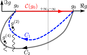
Figure 3: (Color online) Schematic picture of contours that enclose exceptional points. We depict the real cycle $\mathcal{C}(g_{0})$ by a thick line. Note that $\mathcal{C}(g_{0})$ traverses the line $g=\pm\infty$. The concatenation of $\mathcal{C}(g_{0})$ and $C_{1}$ (dashed curve) encloses a single exceptional point $g^{(2)}$, and offers the $1$-EP approximation. On the other hand, the concatenation of $\mathcal{C}(g_{0})$ and $C_{2}$ (dotted curve) encloses two exceptional points $g^{(2)}$ and $g^{(4)}$, and offers the $2$-EP approximation.

VI Eigenspace anholonomy in terms of exceptional points

In this section, we explain the role of exceptional points in the gauge theory that provides a unified formulation of the phase holonomy and the eigenspace anholonomy Cheon-EPL-85-20001 . In particular, we show an evaluation of the holonomy matrix $M(C)$ (See, (31) below), which quantifies the eigenspace anholonomy, using the exceptional points. This confirms our view that the exceptional points constitute a skeleton of the eigenspace anholonomy. To prepare this, we make a brief review of the gauge theory of the eigenspace anholonomy in § VI.1. We show that each exceptional point provides a “local” contribution to $M(C)$ in § VI.2. By collecting these contributions, we conclude this section (§ VI.3).

VI.1 Gauge theory of eigenspace anholonomy

We outline the gauge theory of the eigenspace and phase anholonomies Cheon-EPL-85-20001 . Suppose that the system is initially in an eigenstate $|{}\psi_{\bar{k},n}(g){}\rangle$ and the parameter is adiabatically deformed along a cycle $C$. Let $|{}\psi_{\bar{k},n}(g;C){}\rangle$ denote the final state induced by the adiabatic time evolution along $C$. We assume that the dynamical phase Berry-PRSLA-392-45 is removed from $|{}\psi_{\bar{k},n}(g;C){}\rangle$. A simple way to quantify the eigenspace anholonomy, which concerns about the discrepancy between $|{}\psi_{\bar{k},n}(g){}\rangle$ and $|{}\psi_{\bar{k},n}(g;C){}\rangle$, is to examine the overlapping integral or the holonomy matrix $\langle{}\psi^{\mathrm{L}}_{\bar{k}^{\prime}n^{\prime}}(g){}|{}\psi_{\bar{k}n}(g;C){}\rangle.$ Note that the adiabatic variation of the interaction strength $g$ does not vary $\bar{k}$, which is the quantum number of the center of mass. Hence it suffices to focus on the case $\bar{k}^{\prime}=\bar{k}$:

$$M_{n^{\prime},n}(C)\equiv\langle{}\psi^{\mathrm{L}}_{\bar{k}n^{\prime}}(g){}|{}\psi_{\bar{k}n}(g;C){}\rangle,$$ (30)

which is independent of $\bar{k}$, as is seen below. Also, $M_{n^{\prime},n}(C)$ is non-zero only when the oddness (or evenness) of $\bar{k}$, $n^{\prime}$ and $n$ is the same. Hence $M(C)$ is consist of the even and odd blocks.

A gauge covariant expression of $M(C)$ is

$$M(C)=\mathop{\rm exp}_{\rightarrow}\left(-i\int_{C}A(g)dg\right)\exp\left(i\int_{C}A^{\mathrm{D}}(g)dg\right),$$ (31)

where $\mathop{\rm exp}_{\rightarrow}$ indicates the anti-path-ordered exponential, and $A(g)$ and $A^{\mathrm{D}}(g)$ are gauge connections Cheon-EPL-85-20001 ; Kim-PLA-374-1958

$$\begin{split}A_{n^{\prime},n}(g)&\equiv i\langle{}\psi^{\mathrm{L}}_{\bar{k}n^{\prime}}(g){}|\left[\partial_{g}|{}\psi_{\bar{k},n}(g){}\rangle\right]\\ A^{\mathrm{D}}_{n^{\prime},n}(g)&\equiv\delta_{n^{\prime},n}A_{\bar{k}n^{\prime},\bar{k}n}(g),\end{split}$$ (32)

which are independent of the total momentum $\bar{k}$, too.

Two kinds of gauge invariants are involved in $M(C)$ Tanaka-JPA-45-335305 . One is a permutation matrix and the other is the off-diagonal geometric phases Manini-PRL-85-3067 .

In the following, we impose the parallel transport condition Stone-PRSLA-351-141 for each eigenspace, i.e.,

$$A^{\mathrm{D}}_{n^{\prime},n}(g)=0.$$ (33)

This makes the parametric evolution of the eigenvectors precisely describe the adiabatic time evolution except the dynamical phase. Hence it is also suitable to investigate analytic continuation of the adiabatic parameter for eigenfunction. Regardless of $C$ being closed or open, the parametric evolution of eigenvectors is described by the gauge connection $A{}(g)$ as

$$|{}\psi_{\bar{k},n}(g;C){}\rangle=\sum_{n^{\prime}}|{}\psi_{\bar{k},n^{\prime}}(g){}\rangle\left[\mathop{\rm exp}_{\rightarrow}\left(-i\int_{C}A(g)dg\right)\right]_{n^{\prime}n}.$$ (34)

In particular, the second factor in (31) vanishes

$$M(C)=\mathop{\rm exp}_{\rightarrow}\left(-i\int_{C}A(g)dg\right).$$ (35)

We obtain the gauge connections from (32), (8) and (12). The diagonal elements are

$$A_{n,n}(g)$$ (36)

$$= \begin{cases}\partial_{g}\left[i\ln\left\{a^{(\mathrm{g})}(k)\left(1+\frac{\sin(\pi k)}{\pi k}\right)^{1/2}\right\}\right],&\text{for even $n$, }\\ \partial_{g}\left[i\ln\left\{a^{(\mathrm{e})}(k)\left(1-\frac{\sin(\pi k)}{\pi k}\right)^{1/2}\right\}\right],&\text{for odd $n$ }.\end{cases}$$

The parallel transport condition (33) implies

$$a^{(\mathrm{g})}(k) = a^{(\mathrm{g})}(0)\sqrt{2}\left(1+\frac{\sin(\pi k)}{\pi k}\right)^{-1/2},$$ (37)

$$a^{(\mathrm{e})}(k) = \alpha\sqrt{2}\left(1-\frac{\sin(\pi k)}{\pi k}\right)^{-1/2},$$ (38)

where $\alpha$ is a constant. The off-diagonal elements of the gauge connections are

$$A_{n^{\prime}n}(g)=-i\frac{4}{\pi}\frac{D_{n^{\prime}}(g)D_{n}(g)}{k^{\prime 2}-k^{2}}\left(1-\delta_{n^{\prime}n}\right),$$ (39)

where $k=k_{n}(g)$ and $k^{\prime}=k_{n^{\prime}}(g)$ are assumed, and

$$D_{n}(g)\equiv\begin{cases}\left(1+\frac{\sin(\pi k)}{\pi k}\right)^{-\frac{1}{2}}\cos\frac{\pi k}{2},&\text{for even $n$, }\\ \left(1-\frac{\sin(\pi k)}{\pi k}\right)^{-\frac{1}{2}}{\sin\frac{\pi k}{2}},&\text{for odd $n$. }\end{cases}$$ (40)

We will obtain another expression of $D_{n}(g)$ in Appendix A:

$$D_{n}(g)=d_{n}\frac{k_{n}(g)}{\sqrt{\left\{k_{n}(g)\right\}^{2}+g^{2}+2g/\pi}},$$ (41)

where $d_{n}$ is defined as

$$d_{n}=(-1)^{[n/2]},$$ (42)

and $[x]$ is the maximum integer less than $x$.

VI.2 Contribution from an exceptional point to $M(C)$

We evaluate $M(C)$ (35), deforming the integration contour $C$. The anti-path-ordered exponential in $M(C)$ is decomposed into the contributions from the exceptional points. Here we focus on the contribution from the single exceptional point $g^{(n)}$ ($n>1$). Namely, we will evaluate the anti-path-ordered exponential of the gauge connection along the contour $C^{(n)}=\left\{g^{(n)}+\epsilon e^{i\theta}|\;\theta_{0}\leq\theta\leq\theta_{0}+2\pi\right\}$, which encircles the exceptional point $g^{(n)}$ along the clockwise direction with the radius $\epsilon$ (see figure 4). In particular, we focus on the limit $\epsilon\downarrow 0$, i.e.,

$$M^{(n)}\equiv\lim_{\epsilon\downarrow 0}\mathop{\rm exp}_{\rightarrow}\left(-i\int_{C^{(n)}}A{}(g)dg\right),$$ (43)

in the following.

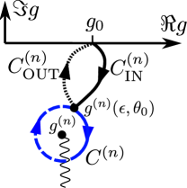
Figure 4: (Color online) Schematic picture of contours for the evaluation of (43) and (57). The circle $C^{(n)}$ encircles an exceptional point $g^{(n)}$ with a radius $\epsilon$ (see the main text). The initial point of the cycle $C^{(n)}$ is denoted by $g^{(n)}(\epsilon,\theta_{0})=g^{(n)}+\epsilon e^{i\theta_{0}}$. Note that $C^{(n)}$ intersects a branch cut (wavy line) that emanates from $g^{(n)}$. The bold and dotted lines that connect $g_{0}$ and $g^{(n)}(\epsilon,\theta_{0})$ are $C^{(n)}_{\rm IN}(g_{0})$ and $C^{(n)}_{\rm OUT}(g_{0})$, respectively.

First, we show that the gauge connection $A{}(g)$ is singular at the exceptional point. Assume that $\epsilon\equiv g-g^{(n)}$ is small. As explained in Sec. IV, the quasi-momenta $k_{n_{\mathrm{b}}}(g)$ and $k_{n}(g)$ are degenerate at $\epsilon=0$, i.e., $g=g^{(n)}$, where $n_{\mathrm{b}}=0$ for even $n$, and $n_{\mathrm{b}}=1$ for odd $n$. In Appendix B, we show that

$$D_{n}(g)D_{n_{\mathrm{b}}}(g)=d_{n}\frac{i\pi^{1/2}k^{(n)}}{2^{3/2}\epsilon^{1/2}}\left[1+\mathcal{O}(\epsilon^{1/2})\right].$$ (44)

On the other hand, (24) implies

$$\left(\left[k_{n}(g)\right]^{2}-\left[k_{n_{\mathrm{b}}}(g)\right]^{2}\right)^{-1}=\frac{\pi^{1/2}}{2^{5/2}k^{(n)}\epsilon^{1/2}}\left[1+\mathcal{O}(\epsilon^{1/2})\right].$$ (45)

Combining these factors, each of which diverges $\mathcal{O}(\epsilon^{-1/2})$ as $\epsilon\to 0$, we find

$$A_{n,n_{\mathrm{b}}}(g)=d_{n}\frac{1}{4\epsilon}\left[1+\mathcal{O}(\epsilon^{1/2})\right].$$ (46)

Accordingly, the gauge connection within the subspace spaned by $n_{\mathrm{b}}$-th and $n$-th eigenstates is

$$\left[\begin{array}[]{cc}A_{n_{\mathrm{b}},n_{\mathrm{b}}}(g)&A_{n_{\mathrm{b}},n}(g)\\ A_{n,n_{\mathrm{b}}}(g)&A_{n_{0},n_{0}}(g)\end{array}\right]=i\frac{d_{n}}{\epsilon}R\left[1+\mathcal{O}(\epsilon^{1/2})\right],$$ (47)

where

$$R\equiv-\frac{1}{4}\left[\begin{array}[]{cc}0&-i\\ i&0\end{array}\right].$$ (48)

The leading term is proportional to $\epsilon^{-1}$ and single-valued around $\epsilon=0$. The next leading term exhibits weaker divergence $\mathcal{O}(\epsilon^{-1/2})$ and multiple-valuedness. Other matrix elements of (32) exhibit, at most, the weaker divergence $\mathcal{O}(\epsilon^{-1/2})$.

We examine $M^{(2)}$ by expanding the anti-path-ordered exponential in (43):

$$M^{(2)} = \lim_{\epsilon\downarrow 0}\mathop{\mathcal{P}}_{\rightarrow}\left[1-i\int_{C^{(2)}}A(g)dg\right.$$ (49)

$$\qquad\qquad\left.-\frac{1}{2}\int_{C^{(2)}}A(g_{1})dg_{1}\int_{C^{(2)}}A(g_{2})dg_{2}\right.$$

$$\qquad\qquad\left.+\dots\right],$$

where $\mathop{\mathcal{P}}_{\rightarrow}$ indicates the anti-path ordering product of matrices. From the argument above, the dominant part of the gauge connection has a block-diagonal structure

$$A{}(g^{(2)}+\epsilon)=-\frac{i}{{\epsilon}}\left[\begin{array}[]{c|c}R&0\\ \hline\cr 0&0\\ \end{array}\right]+\mathcal{O}(\epsilon^{-\frac{1}{2}}),$$ (50)

where the matrix representation involves only the subspace that consists of $|{}\psi_{0,n}(g){}\rangle$ with even $n$($\geq 0$). Since the circumference of $C^{(2)}$ is $2\pi\epsilon$, only the leading term in (50) contributes to $M^{(2)}$:

$$M^{(2)}=\left[\begin{array}[]{c|c}\exp\left(-i2\pi R\right)&0\\ \hline\cr 0&1\\ \end{array}\right].$$ (51)

It is straightforward to see

$$\exp\left(-i2\pi R\right)=\left[\begin{array}[]{cc}0&-1\\ 1&0\end{array}\right]$$ (52)

from (48). Hence we obtain

$$M^{(2)}=\left[\begin{array}[]{cc|c}0&-1&0\\ 1&0&0\\ \hline\cr 0&0&1\end{array}\right],$$ (53)

which describes the parametric evolution of eigenvectors along $C^{(2)}$. The bound state $|{}\psi_{0,0}(g){}\rangle$ evolves into $|{}\psi_{0,2}(g){}\rangle$. The partner $|{}\psi_{0,2}(g){}\rangle$ evolves into $-|{}\psi_{0,0}(g){}\rangle$, where an extra phase factor $(-1)$ is acquired. Other eigenvectors are remain unchanged.

It is straightforward to obtain $M^{(n)}$ for an arbitrary $n$($>1$)

$$\begin{split}M^{(n)}_{n^{\prime\prime}n^{\prime}}&=d_{n}\left(\delta_{n^{\prime\prime}n_{\mathrm{b}}}\delta_{n^{\prime}n}-\delta_{n^{\prime\prime}n}\delta_{n^{\prime}n_{\mathrm{b}}}\right)\\ &\qquad+(1-\delta_{n^{\prime\prime}n_{\mathrm{b}}})(1-\delta_{n^{\prime\prime}n})\delta_{n^{\prime\prime}n^{\prime}}.\end{split}$$ (54)

We depict a few of them:

$$M^{(4)}=\left[\begin{array}[]{ccc|c}0&0&1&0\\ 0&1&0&0\\ -1&0&0&0\\ \hline\cr 0&0&0&1\end{array}\right],\qquad M^{(6)}=\left[\begin{array}[]{cccc|c}0&0&0&-1&0\\ 0&1&0&0&0\\ 0&0&1&0&0\\ 1&0&0&0&0\\ \hline\cr 0&0&0&0&1\end{array}\right].$$ (55)

VI.3 Combining multiple-EP contributions

Let us examine the analytic continuation of eigenvector $|{}\psi_{0,n^{\prime}}(g_{0}){}\rangle$, where $g_{0}$ is real and $n^{\prime}$ is even. We extend $|{}\psi_{0,n^{\prime}}(g_{0}){}\rangle$ along the cycle (see figure 4)

$$C^{(n)}(g_{0})=C^{(n)}_{\mathrm{IN}}(g_{0})\circ{}C^{(n)}_{\mathrm{EP}}\circ{}C^{(n)}_{\mathrm{OUT}}(g_{0})$$ (56)

($n>1$), where $a\circ b$ indicates the concatenation of paths $a$ and $b$. We note that all eigenvectors remain unchanged against the parametric evolution along $C^{(n)}_{\mathrm{IO}}(g_{0})\equiv C^{(n)}_{\mathrm{IN}}(g_{0})\circ C^{(n)}_{\mathrm{OUT}}(g_{0})$, because $C^{(n)}_{\mathrm{IO}}(g_{0})$ encloses no branch point (figure 4). Hence, from (34), $|{}\psi_{0,n}(g_{0};C^{(n)}(g_{0})){}\rangle$ has the following expression

$$|{}\psi_{0,n}(g_{0};C^{(n)}(g_{0})){}\rangle=\sum_{n^{\prime\prime}}|{}\psi_{0,n^{\prime\prime}}(g_{0}){}\rangle M^{(n)}_{n^{\prime\prime},n^{\prime}}.$$ (57)

Next, we consider the effect of two exceptional points $g^{(2)}$ and $g^{(4)}$ using a contour $C^{(2,4)}\equiv C^{(2)}(g_{0})\circ C^{(4)}(g_{0})$ (see, figures 3 and 4). To carry out this, let us extend the eigenvectors in (57) with $n=2$ along $C^{(4)}(g_{0})$. We find

$$|{}\psi_{0,n}(g_{0};C^{(2,4)}(g_{0})){}\rangle=\sum_{n^{\prime\prime}}|{}\psi_{0,n^{\prime\prime}}(g_{0};C^{(4)}(g_{0})){}\rangle M^{(2)}_{n^{\prime\prime},n^{\prime}}.$$ (58)

Hence we obtain, using (57) with $n=4$,

$$|{}\psi_{0,n}(g_{0};C^{(2,4)}(g_{0})){}\rangle=\sum_{n^{\prime\prime}}|{}\psi_{0,n^{\prime\prime}}(g_{0}){}\rangle M^{(2,4)}_{n^{\prime\prime},n^{\prime}},$$ (59)

where

$$M^{(2,4)}=M^{(4)}M^{(2)}.$$ (60)

Furthermore, we examine the analytic continuation of $|{}\psi_{0,n}(g_{0}){}\rangle$ along

$$C^{(2,\dots,2m)}(g_{0})\equiv C^{(2,\dots,2m-2)}(g_{0})\circ C^{(2m)}(g_{0})$$ (61)

($m>1$). In a similar way above, we find

$$|{}\psi_{0,n}(g_{0};C^{(2,\dots,2m)}(g_{0})){}\rangle=\sum_{n^{\prime\prime}}|{}\psi_{0,n^{\prime\prime}}(g_{0}){}\rangle M^{(2,\dots,2m)}_{n^{\prime\prime},n^{\prime}},$$ (62)

where

$$M^{(2,\dots,2m)}=M^{(2m)}M^{(2,\dots,2m-2)}.$$ (63)

As shown in Appendix C, we obtain

$$M^{(2,\dots,2m)}_{n^{\prime\prime},n^{\prime}}$$ (64)

$$= \sum_{m^{\prime}=0}^{m-1}\delta_{n^{\prime\prime},2(m^{\prime}+1)}\delta_{n^{\prime},2m^{\prime}}+(-1)^{m}\delta_{n^{\prime\prime},0}\delta_{n^{\prime},2m}$$

$$\qquad+\prod_{m^{\prime}=0}^{m}\left(1-\delta_{n^{\prime\prime},2m^{\prime}}\right)\delta_{n^{\prime\prime},n^{\prime}},$$

where the first and second term describe the shift of eigenstates $(0,\dots,2m-2)\mapsto(2,\dots,2m)$, and the shift of eigenstate $2m\mapsto 0$ with a phase factor $(-1)^{m}$. The other eigenstates remain unchanged by the closed contour $C^{(2,\dots,2m)}(g_{0})$. Hence this contour accurately describes the shift of eigenstates up to $(2m-2)$-th excited states. In this sense, $C^{(2,\dots,2m)}(g_{0})$ emulates $C$ in the limit $m\to\infty$ as for the exotic quantum holonomy induced by $\mathcal{C}(g_{0})$ along the real axis of $g$, i.e.,

$$M^{(2,\dots,2m)}\to M\left(\mathcal{C}(g_{0})\right)$$ (65)

as $m\to\infty$.

VII Discussion

First, we compare the present result with Ref. Kim-PLA-374-1958 , where the correspondence between the exotic quantum holonomy and exceptional points is examined in families of quantum kicked spin-$\frac{1}{2}$. First of all, because a kicked spin is a periodically driven system, the exotic quantum holonomy of the eigenvalues and the eigenvectors of Floquet operator, which is the time evolution operator during the period of a driving force, is investigated. Hence the physical context of the exotic quantum holonomy is slightly different from the one in autonomous systems. On the other hand, these two models have the same relationship between the quantum holonomy and the exceptional points, as a whole. For example, the multiple-valuedness of eigenvalues and eigenvectors is governed by the exceptional points. The non-Abelian gauge connection has a $\epsilon^{-1}$-divergence around an exceptional point (see (47)), where $\epsilon$ is the distance from the exceptional point in the parameter space. This divergence comprises the permutation of eigenvectors against a tiny loop around the exceptional point (see (53)). However, we find a subtle difference on the analyticity of the gauge connection. As for the kicked spin, the gauge connection is single-valued in the parameter space. We may say that the gauge connection has a degree-$1$ pole at an exceptional point of the kicked spin. On the other hand, as for the gauge connection of two-body Lied-Liniger model, an exceptional point is not only a divergent point, but also a branch point. However the multiple-valuedness appears only in the higher-order correction terms about $\epsilon$ (see (47)).

Second, it is certain that we should see whether the present observations apply to Lieb-Liniger model with an arbitrary number of particles, as we focus on the two-body case. We may expect that a similar scenario on the interplay of the exotic quantum holonomy and the exceptional points can be applicable. For example, according to the strong coupling expansion explained in Section IV, the degree of exceptional points is $2$ and each exceptional point connects the ground state and an excited state, regardless of the number of particles Ushveridze-JPA-21-955 . On the other hand, however, there remain subtle points. For example, as for two-body case, the repetitions of the adiabatic cycle $\mathcal{C}(g_{0})$ and its inverse connect all eigenstates once we specify the total momentum. We call the collection of such eigenstates a family Yonezawa-up-20130 . From the present analysis, a family corresponds to a Riemann surface of eigenenergy. The analytic continuation of the interaction strength $g$ can connect any pair of eigenstates in a family. However, as discovered in Ref. Yonezawa-up-20130 , there is an infinite number of families in three-body Lieb-Liniger model. For now, whether or not a family corresponds to a Riemann surface of eigenenergy is unknown, because several families might be connected in a region far from the real axis of a Riemann surface. In other words, the question is open as to whether there is any exceptional point that is “inaccessible” by the real cycles. Suppose that there is no such inaccessible exceptional point. This implies one-to-one correspondence between a family and a Riemann surface. Although this might suggest that the exceptional point picture obtained for the two body case is applicable to an arbitrary number of particles, another question is raised. There is only a single Riemann surface for a given total momentum when the number of particles is two. The number of Riemann surfaces, however, is infinite for the number of particle is three. We do not know how such a proliferation of Riemann surfaces against the increment of the number of particles is possible.

VIII Summary

We have shown the direct link between the exotic quantum holonomy in eigenenergies and eigenspaces, and the exceptional points, which are degeneracy points in the complexified parameter space in two-body Lieb-Liniger model. With the help of Bethe ansatz, we examine the Riemann surface of quasi-momentum. All exceptional points in the lower half plane participate the eigenenergy anholonomy. Also the non-Abelian gauge connection introduced for the eigenspace anholonomy exhibits divergent behavior around the exceptional point as well as tiny multiple-valuedness correction. The exceptional points offer building blocks of the eigenspace anholonomy. It remains to be seen how the current result is to be extended to systems with an arbitrary number of particles.

Appendix A $D$-function

We show how we obtain (41). In the following, we assume that $n$ is even. It is straightforward to obtain a similar argument for odd $n$. Using the fact that $k=k_{n}(g)$ satisfies (3), we find that the numerator and the denominator of (40) satisfy

$$\cos\frac{z\pi}{2}=\pm\sqrt{\frac{k^{2}}{k^{2}+g^{2}}},$$ (66)

and

$$\sqrt{1+\frac{\sin(\pi k)}{\pi k}}=\sqrt{\frac{\pi(k^{2}+g^{2})+2g}{\pi(k^{2}+g^{2})}},$$ (67)

respectively. Hence we obtain

$$D_{n}(g)=\pm\frac{k_{n}(g)}{\sqrt{\{k_{n}(g)\}^{2}+g^{2}+2g/\pi}}.$$ (68)

There remains the ambiguity of sign. It is chosen so as to be consistent with the behavior of (40) in the real axes:

$$D_{n}(g)=(-1)^{n/2}\frac{k_{n}(g)}{\sqrt{\{k_{n}(g)\}^{2}+g^{2}+2g/\pi}}.$$ (69)

Hence we obtain (41) in the main text.

Appendix B A derivation of (44)

We examine the singular behavior of the gauge connection (32) around the exceptional point $g^{(n)}$ ($n>1$). We assume that $\epsilon\equiv g-g^{(n)}$ is small. Two quasi-momenta $k_{n}(g)$ and $k_{n_{\mathrm{b}}}(g)$ degenerates at $(\epsilon,k)=(0,k^{(n)})$, where $n_{\mathrm{b}}=0$ for even $n$, and $n_{\mathrm{b}}=1$ for odd $n$. We summarize (24) and (25)

$$\begin{split}k_{n}(g)&=k^{(n)}+\left(\frac{2}{\pi}\epsilon\right)^{1/2}+\mathcal{O}(\epsilon).\\ k_{n_{\mathrm{b}}}(g)&=k^{(n)}-\left(\frac{2}{\pi}\epsilon\right)^{1/2}+\mathcal{O}(\epsilon).\end{split}$$ (70)

We choose that the branch cut emanating from $g^{(n)}$ is parallel to the imaginary axis, and is confined within the lower half plane. Namely, we suppose that

$$-\frac{\pi}{2}<{\rm Arg}\;\epsilon\leq\frac{3\pi}{2}$$ (71)

in the Riemann sheet where we are working.

We will examine

$$r_{n}(g)\equiv\left\{k_{n}(g)\right\}^{2}+g^{2}+2g/\pi$$ (72)

in order to evaluate $D_{n}(g)=d_{n}k_{n}(g)/\sqrt{r_{n}(g)}$ around $g^{(n)}$. We start from the real axis, where ${\rm Arg}\;r_{n}(g)=0$ holds. Hence we expect

$$-\pi<{\rm Arg}\;r_{n}(g)\leq\pi$$ (73)

holds around the region between the real axis and $g^{(n)}$, as ${\rm Arg}\;r_{n}(g)$ has no singular point there. We examine ${\rm Arg}\;\;r_{n_{\mathrm{b}}}(g)$ in a similar way. As for real $g$, we have $r_{n_{\mathrm{b}}}(g)>0$ for $g>-(2/\pi)n_{\mathrm{b}}$ and $r_{n_{\mathrm{b}}}(g)<0$ for $g<-(2/\pi)n_{\mathrm{b}}$. Note that $\sqrt{r_{n_{\mathrm{b}}}(g)}$ has a branch point at $g=0$, and the corresponding branch cut locates at the imaginary axis within the upper half plane. So we choose ${\rm Arg}\;r_{n_{\mathrm{b}}}(g)=0$ for $g>-(2/\pi)n_{\mathrm{b}}$ and ${\rm Arg}\;r_{n_{\mathrm{b}}}(g)=-\pi$ for $g<-(2/\pi)n_{\mathrm{b}}$. Hence we expect that

$$-\frac{3\pi}{2}<{\rm Arg}\;r_{n_{\mathrm{b}}}(g)\leq\frac{\pi}{2}$$ (74)

is valid in the region between the real axis and $g^{(n)}$.

We move to the vicinity of the exceptional point $g^{(n)}$, where we obtain

$$r_{n}(g) = \frac{2^{3/2}}{\pi^{1/2}}k^{(n)}\epsilon^{1/2}\left[1+\mathcal{O}(\epsilon^{1/2})\right],$$ (75)

$$r_{n_{\mathrm{b}}}(g) = -\frac{2^{3/2}}{\pi^{1/2}}k^{(n)}\epsilon^{1/2}\left[1+\mathcal{O}(\epsilon^{1/2})\right].$$ (76)

Note that ${\rm Arg}\;\;r_{n}(g)$ and ${\rm Arg}\;\;r_{n_{\mathrm{b}}}(g)$ are singular at $g^{(n)}$, i.e., $\epsilon=0$. From $g^{(n)}$, the real axis is located in the direction ${\rm Arg}\;\epsilon=\pi/2$, where (73) and  (74) are expected to be valid. We choose ${\rm Arg}\;k^{(n)}$ so as to satisfy

$$-\pi<\frac{\pi}{4}+{\rm Arg}\;k^{(n)}\leq\pi,$$ (77)

in order to be consistent with (73). On the other hand, there remains ambiguity of ${\rm Arg}\;r_{n_{\mathrm{b}}}(g)={\rm Arg}\;(-1)+\frac{\pi}{4}+{\rm Arg}\;k^{(n)}$. We resolve this using (77) and (74). We conclude

$${\rm Arg}\;r_{n_{\mathrm{b}}}(g)=-\pi+\frac{1}{2}{\rm Arg}\;\epsilon+{\rm Arg}\;k^{(n)},$$ (78)

which implies (44) in the main text.

Appendix C A proof of (64)

We prove (64) by induction. Note that, as for $m=1$, (53) implies Eq. (64). Hence it suffices to prove (64) for $m=m^{\prime}+1$ using the assumption that (64) holds for $m=m^{\prime}$($>1$). For simplicity, $m^{\prime}$ is denoted by $m$. From the recursion relation (63), we have

$$M^{(2,\dots,2m+2)}_{n^{\prime\prime},n^{\prime}}=\sum_{n}M^{(2m+2)}_{n^{\prime\prime}n}M^{(2,\dots,2m)}_{nn^{\prime}}.$$ (79)

We find from (54)

$$M^{(2,\dots,2m+2)}_{n^{\prime\prime},n^{\prime}} = (-1)^{m+1}\delta_{n^{\prime\prime}0}M^{(2,\dots,2m)}_{2(m+1),n^{\prime}}$$

$$\qquad+(-1)^{m}\delta_{n^{\prime\prime},2(m+1)}M^{(2,\dots,2m)}_{0n^{\prime}}$$

$$\qquad+(1-\delta_{n^{\prime\prime}0})(1-\delta_{n^{\prime\prime}2(m+1)})M^{(2,\dots,2m)}_{n^{\prime\prime}n^{\prime}}.$$

Hence, (64) implies

$$M^{(2,\dots,2m+2)}_{n^{\prime\prime},n^{\prime}} = \sum_{m^{\prime}=0}^{m}\delta_{n^{\prime\prime},2(m^{\prime}+1)}\delta_{n^{\prime},2m^{\prime}}$$

$$\qquad+(-1)^{m+1}\delta_{n^{\prime\prime},0}\delta_{n^{\prime},2(m+1)}$$

$$\qquad+\left[\prod_{m^{\prime}=0}^{m+1}\left(1-\delta_{n^{\prime\prime},2m^{\prime}}\right)\right]\delta_{n^{\prime\prime},n^{\prime}}.$$

Hence the proof of (64) is completed.

References

- (1) Born M and Fock V 1928 Z. Phys. 51 165
- (2) Kato T 1950 J. Phys. Soc. Japan 5 435
- (3) Longuet-Higgins H C 1975 Proc. R. Soc. London A 344 147
- (4) Mead C and Truhlar D G 1979 J. Chem. Phys. 70 2284
- (5) Berry M V 1984 Proc. R. Soc. London A 392 45
- (6) Wilczek F and Zee A 1984 Phys. Rev. Lett. 52 2111
- (7) Bohm A, Mostafazadeh A, Koizumi H, Niu Q and Zwanziger Z 2003 The Geometric Phase in Quantum Systems (Berlin: Springer)
- (8) Cheon T 1998 Phys. Lett. A 248 285
- (9) Tanaka A and Miyamoto M 2007 Phys. Rev. Lett. 98 160407
- (10) Kim S W, Cheon T and Tanaka A 2010 Phys. Lett. A 374 1958
- (11) Kato T 1980 Perturbation Theory for Linear Operators (Berlin: Springer-Verlag) chap II corrected printing of the second ed
- (12) Heiss W D and Steeb W H 1991 J. Math. Phys. 32 3003
- (13) Heiss W 2004 Czechoslovak Journal of Physics 54 1091
- (14) See, e.g., Bender C, Fring A, Günther U and Jones H 2012 “Quantum physics with non-Hermitian operator”, J. Phys. A: Math. Theor. 45 440301
- (15) See, e.g., Moiseyev N 2011 Non-Hermitian Quantum Mechanics (New York: Cambridge Univ. Press)
- (16) Lieb E H and Liniger W 1963 Phys. Rev. 130 1605
- (17) Ushveridze A G 1988 J. Phys. A. 21 955
- (18) Yonezawa N, Tanaka A and Cheon T 2013 Phys. Rev. A 87 062113
- (19) Dürr S, García-Ripoll J J, Syassen N, Bauer D M, Lettner M, Cirac J I and Rempe G 2009 Phys. Rev. A 79 023614
- (20) Olshanii M 1998 Phys. Rev. Lett. 81 938
- (21) Haller E, Gustavsson M, Mark M J, Danzl J G, Hart R, Pupillo G and Nägerl H C 2009 Science 325 1224
- (22) Haller E, Mark M J, Hart R, Danzl J G, Reichsöllner L, Melezhik V, Schmelcher P and Nägerl H C 2010 Phys. Rev. Lett. 104 153203
- (23) Cheon T and Tanaka A 2009 Europhys. Lett. 85 20001
- (24) Tanaka A, Cheon T and Kim S W 2012 J. Phys. A: Math. Theor. 45 335305
- (25) Manini N and Pistolesi F 2000 Phys. Rev. Lett. 85 3067
- (26) Stone A J 1976 Proc. R. Soc. London A 351 141
- (27) Arnold V I 1991 Selecta Mathematica, New Series 1 1
- (28) Mailybaev A A. Kirillov O N, and Seyranian A P 2005, Phys. Rev. A 72 014104
- (29) Dietz B, Harney H L, Kirillov O N, Miski-Oglu M, Richter A and Schäfer F 2011, Phys. Rev. Lett. 106 150403