Observing coronal nanoflares in active region moss

Abstract

The High-resolution Coronal Imager (Hi-C) has provided Fe XII 193Å images of the upper transition region moss at an unprecedented spatial ($\sim 0.3-0.4$^′′) and temporal (5.5s) resolution. The Hi-C observations show in some moss regions variability on timescales down to $\sim 15$ s, significantly shorter than the minute scale variability typically found in previous observations of moss, therefore challenging the conclusion of moss being heated in a mostly steady manner. These rapid variability moss regions are located at the footpoints of bright hot coronal loops observed by SDO/AIA in the 94Å channel, and by Hinode/XRT. The configuration of these loops is highly dynamic, and suggestive of slipping reconnection. We interpret these events as signatures of heating events associated with reconnection occurring in the overlying hot coronal loops, i.e., coronal nanoflares. We estimate the order of magnitude of the energy in these events to be of at least a few $10^{23}$ erg, also supporting the nanoflare scenario. These Hi-C observations suggest that future observations at comparable high spatial and temporal resolution, with more extensive temperature coverage are required to determine the exact characteristics of the heating mechanism(s).

1 Introduction

Coronal heating is one of the central problems in solar physics, and the detailed characteristics of the processes converting magnetic into thermal energy are still hotly debated (see e.g., Klimchuk, 2006; Reale, 2010, for reviews). Heating processes are likely to occur on small spatial and temporal scales, which are difficult to access with the typical resolution of present instrumentation. The spatial and temporal characteristics of heating in active regions (ARs) have been investigated by indirectly inferring constraints from the spatial, temporal and thermal properties of the plasma from imaging and spectral data, and comparing them with predictions of different heating models (e.g., Reale et al., 2009a, b; McTiernan, 2009; Hansteen et al., 2010; Testa et al., 2011; Tripathi et al., 2011; Winebarger et al., 2011b; Warren et al., 2012). One of the candidate processes for coronal heating is the nanoflare model, where the heating is produced by reconnection due to braiding of coronal magnetic field lines caused by random motions of the loop footpoints in the photosphere (Parker, 1988; Cirtain et al., 2013). Several models have been developed assuming nanoflare events to occur in unresolved loop strands (e.g., Cargill, 1994; Cargill & Klimchuk, 1997), and provide a viable interpretation of various coronal AR observations which are constraining the spatial distribution and frequency of the heating events (e.g., Reale et al., 2011; Warren et al., 2011). However, past observations provide only limited constraints to the models, and higher quality observations are crucial to test the models. We note that scenarios alternative to Parker’s have been proposed, which can also produce nanoflare-like heating (e.g., van Ballegooijen et al., 2011; De Pontieu et al., 2011).

Heating events are difficult to investigate in the corona, where conduction is extremely efficient in smoothing out gradients, therefore many studies have focused on “moss”, i.e., the upper transition region (TR) layer of high pressure loops in active regions, which is very bright in narrowband EUV images sensitive to $\sim 1$ MK emission (e.g., Peres et al., 1994; Fletcher & De Pontieu, 1999; Berger et al., 1999b; De Pontieu et al., 1999; Martens et al., 2000). Revealed first by recent high spatial resolution X-rays and EUV narrowband coronal imagers, such as NIXT (Golub et al., 1990) and TRACE (Handy et al., 1999), the moss is very bright in cool EUV bands (e.g., 171Å and 193Å). Moss is generally relatively free from line-of-sight (LOS) confusion due to the lack of overlying coronal emission, since the overlying coronal loops are hotter (few MK) and only weakly emitting in cool EUV narrowbands. The moss has been found to have typical temperatures of 0.6-1.5 MK, densities of the order of $10^{10}$ cm^-3, and thickness of about 1-3 Mm (e.g., Fletcher & De Pontieu, 1999; Berger et al., 1999b; Warren et al., 2008b). Studies using imaging and spectral observations of moss have found relatively low level temporal variability, placing constraints on the frequency and distribution of intensity of heating events, and it has often been interpreted as an indication of quasi-steady heating of the moss and therefore of the associated AR core loops (Antiochos et al., 2003; Brooks et al., 2009; Tripathi et al., 2010). However, spatial and temporal averaging can significantly influence the results found for moss variability, as we show here.

In this Letter, we investigate the properties of moss by using EUV imaging data of the High-resolution Coronal Imager (Hi-C) instrument, which are characterized by unprecedented spatial ($\sim 0.3-0.4$^′′) and temporal ($\sim 5.5$ s) resolution. Hi-C, launched on a sounding rocket on 2012 July 11, has provided about 5 minutes of EUV observations of coronal and TR plasma in a 6.8 arcmin $\times$ 6.8 arcmin field of view, in a narrow passband very similar to the SDO/AIA 193Å band (Cirtain et al., 2013). We show that the spatial and temporal resolution of Hi-C data reveal moss variability on very short timescales, contrary to previous findings, and suggesting a more episodic nature of the heating compared to what was previously thought. These rapid and intense brightenings are found at the footpoints of hot (several MK) loops, and we interpret them as the signature of heating episodes due to reconnection higher up in the corona, i.e., coronal nanoflares. In order to investigate the relation of the high variability in the moss with the overlying coronal emission and surface magnetic field we analyze simultaneous observations from Hi-C, SDO/AIA (Lemen et al., 2012), Hinode/XRT (Golub et al., 2007) and SDO/HMI (Scherrer et al., 2012), as described in Section 2. In Section 3 we present the results of our analysis of the temporal variability in the moss as observed by Hi-C, and spatial correlations with hotter corona emission and photospheric magnetic field. We discuss our findings and draw our conclusions in Section 4.

2 Observations

We analyze Hi-C observations ($\sim 0.103$^′′ pixel^-1) of AR 11520 on 2012 July 11 around 18:53UT. Figure 1 shows the region we selected ($\sim 160$^′′$\times 310$^′′) from the full field of view, to focus on the properties of moss regions. We also analyze simultaneous imaging data of the same region in SDO/AIA EUV narrowbands ($\sim 0.6$^′′ pixel^-1, 12 s cadence), and in Hinode/XRT Ti-poly filter ($\sim 1$^′′ pixel^-1, 15 s cadence). The AIA and XRT data have been processed with the aia_prep and xrt_prep routines respectively, available as a part of SolarSoft.

The AIA, XRT, and HMI data have been rescaled to the Hi-C spatial resolution, corrected for solar rotation, and rotated and transposed to match the Hi-C data. A time series in each band, matching the higher Hi-C temporal resolution, has been created by taking the corresponding image closest in time to the Hi-C observing times. For XRT we combined short and long exposure images to obtain the best signal-to-noise ratio in both dark and bright regions, while avoiding saturation. The data from different instruments have been carefully coaligned by applying cross-correlation procedures. AIA and XRT data, averaged over the duration of the Hi-C observations, as well as an HMI data are shown together with Hi-C data in Figure 1.

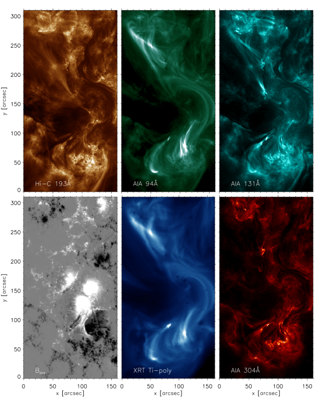
Figure 1: Hi-C, SDO and Hinode/XRT observations of AR 11520 on 2012 July 11. We show images obtained by averaging intensities in the interval approximately between 18:52:50UT and 18:55:30UT. Solar north is to the right, and solar east is down. Top row, left to right: Hi-C 193Å passband, SDO/AIA 94Å and 131Å passbands. Bottom row, left to right: SDO/HMI magnetic field, Hinode/XRT Ti-poly, SDO/AIA 304Å.

The comparison of the images taken by the different instruments shows several moss regions, which are the brightest features in the Hi-C 193Å and AIA 304Å and 131Å images, while in XRT and AIA 94Å coronal loops tend to be the most prominent features. Though the AIA 94Å channel is sensitive to both cool ($\sim 1$ MK) and hot ($\sim 6$ MK) emission (e.g., Boerner et al., 2012; Testa et al., 2012), for these loops the AIA 94Å emission is dominated by Fe xviii emission as supported by the comparison of the AIA coronal channels (according to the method of Testa & Reale, 2012), their temporal evolution, and the close morphological correspondence with the XRT loops.

3 Results

The high spatial and temporal resolution observations of Hi-C show a variety of spatial and temporal scales. Cirtain et al. (2013) investigated brightening in twisted loops (located around $[x,y]\sim[70,80]$^′′ in Figure 1) interpreted as a result of energy release due to fine-scale magnetic field braiding. Close inspection of the Hi-C movies (Movie 1 and 2) shows that a subset of moss regions are characterized by striking temporal variability dominated by localized short duration brightenings ($\sim 15-20$ s). These timescales are significantly shorter than for the typical moss variability that previous studies found on timescales of the order of minutes, and interpreted as due to absorption of EUV emission by chromospheric dynamic fibrils (De Pontieu et al., 2003a, b).

We applied an analysis to the Hi-C time series to single out these regions where brightenings on short timescales occur, characterize the properties of these regions, and investigate the reasons for their strikingly enhanced temporal variability. We spatially rebinned the Hi-C data to the level of the effective spatial resolution, and derived time series of the running difference of the rebinned data. We then apply an algorithm calculating the number of zero crossings of the running difference lightcurves. Finally we obtain a mask of the points where the number of zero crossing is above a certain threshold, since we want to highlight regions characterized by episodic brightenings, i.e., where the lightcurve increases and then decreases to roughly pre-brightening levels, as opposed to steady increases on long timescales. We also impose that the level of variability in intensity is above a given threshold above the average intensity. We explored a small range of spatial rebinning scales, temporal scales for the running difference, and significance of variability. Figure 2 (left panel) shows the map resulting from our temporal analysis (red), calculated using a factor 4 spatial rebin, a running difference calculated over 3 time steps ($\sim 16.5$s), and significance above $4\sigma$. The map is superimposed on the Hi-C data (blue) and the AIA 94Å data (green).

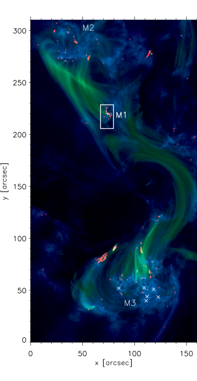
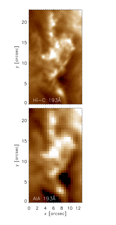
Figure 2: Left: 3 color image combining Hi-C data (blue), SDO/AIA 94Å data (green), and a mask highlighting regions with high level of variability in the Hi-C time series (red; see text for details). The white crosses mark moss locations outside high variability areas which we select for comparison with the rapidly varying moss (Figure 4). Right: 193Å Hi-C (top; $\sim 0.1$^′′ pixel^-1) and AIA (bottom; $\sim 0.6$^′′ pixel^-1) images of the rapid variability moss region M1 (white box in left panel), clearly showing the significantly different spatial resolution of the two instruments.

This map confirms the impression from the visual inspection of the time series, showing a high concentration of locations characterized by high variability on small time scales in the moss region M1 (white box in Figure 2). We note that there appears to be a close correspondence of the rapid variability regions with the brightest areas in the AIA 304Å image. The map of high variability regions also includes a few isolated features in both large moss regions in the field of view (labeled M2, and M3), as well as the reconnection event studied by Cirtain et al. (2013) (at $[x,y]\sim[70,80]$), and some other coherent events like apparent flows (e.g., around $[x,y]\sim[110,90]$ and $[x,y]\sim[115,280]$; see Movie 1). In the following we focus on the very prominent short scale variability in M1.

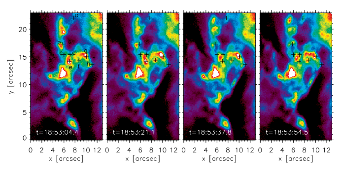
Figure 3: Hi-C images of M1, at four different times, at about 16.5s interval from one another, showing large variations on time scales of about 15-30s in some locations. We label a few selected locations for which we show the Hi-C lightcurves in Figure 4.

The comparison of Hi-C and AIA 193Å images of the moss region M1 (Figure 2, right panels), clearly illustrates the significant improvement of Hi-C in spatial resolution. In Figure 3 we show four images of the high variability moss region M1 at about 16.5s cadence. The high variability is clearly evident already with this limited temporal sampling. A few locations, showing rapid temporal variability, as indicated by the temporal analysis described above, are marked by crosses and labeled, and their lightcurves are shown in Figure 4. For comparison, we also show sample lightcurves for 6 moss locations not characterized by rapid variability (marked in Figure 2).

Figure 4: Hi-C normalized lightcurves for 8 locations labeled ($a-h$) in Figure 3, and for 6 moss locations marked in Figure 2 not characterized by rapid variability (bottom right panel). The lightcurves are obtained by integrating the intensity in a 3 pixel $\times$ 3 pixel area (i.e., comparable with effective spatial resolution of the instrument).

As evident from Figure 1 and 2, the rapidly variable moss region is located at the footpoints of the hottest coronal loops in the AR, which are bright in the AIA 94Å and XRT images. Inspection of the longer time series of AIA images (see Movie 3) indicates that these loops become brighter relatively shortly before the start of Hi-C observations ($\sim 20$min) and the whole coronal loop configuration is highly dynamic. Sets of loops connecting the moss region M2 with M1 appear to be crossing in the plane of the sky. The area where the hot loops appear to cross (around $[x,y]\sim[50,250]$) shows an increase in brightness that is followed by increased brightness along the entire length of loops. The time series of the magnetic field from HMI and of the coronal emission in AIA bands (Movie 3 and 4) support a scenario in which the pre-existing configuration of coronal loops between M1 and the conjugate footpoints, M2, are impacted by emerging flux, as evidenced by the brightening of the loops connecting the right-end area of M2 to this emerging flux region. These hot loops are rapidly evolving, and the apparent displacement of their footpoints towards M1 supports a slipping reconnection scenario as in Aulanier et al. (2007). This reconnection process might explain the brightening of all hot loops anchored to the moss region M2, which is observed simultaneously with the apparent footpoint motion. We discuss in the following the possible implications of these findings.

4 Discussion and Conclusions

In this Letter we have presented observations of active region moss with the Hi-C narrowband EUV imager. The unprecedented combination of high spatial and temporal resolution of Hi-C shows that the moss is structured down to small spatial scales, like the chromosphere (De Pontieu et al., 2003b), and it reveals high levels of temporal variability. This challenges previous findings of moss steady emission (Antiochos et al., 2003; Brooks et al., 2009). Hi-C shows moss areas characterized by slow variability, on typical timescales of minutes, analogous to previous findings (De Pontieu et al., 2003a, b), but it also shows moss locations with high intensity brightenings on very short timescales (down to $\sim 15$ s).

We investigated the characteristics of these rapid variability regions which might explain their distinctively higher temporal variability compared to other moss. We found that these rapid variability regions show an intriguing correlation with the brightest 304Å emission, and they occur at the footpoints of the hottest loops ($\sim 6$ MK), which are brightening after flux emergence is observed. As shown in section 3, the evolution of the coronal configuration of these hot loops is suggestive of slipping reconnection. Even if we cannot exclude heating in the TR region, these observed correlations with the magnetic and coronal features suggest that the rapid moss variability is due to reconnection events and resulting energy release occurring in the corona, i.e., to coronal nanoflares. The energy transport to the TR layers can be due to either thermal conduction and/or to beams of non-thermal particles accelerated at the reconnection site (e.g., Brosius, 2012; Brosius & Holman, 2012). We note that the signal-to-noise ratio and temporal resolution of the AIA 94Å images are too low to resolve these heating events in the corona (as expected on the basis of simulations of nanoflare heated multi-stranded loops; e.g., Reale & Orlando 2008; Bradshaw & Klimchuk 2011) and to investigate their temporal correlations with the events Hi-C observes at lower temperatures at the loop footpoints.

Since the TR emission timescales depends on the timescale of evolution of pressure (see e.g., Klimchuk et al., 2008), the extremely short timescales for the moss brightenings imply that the associated heating events must last less than $\sim 15$s (comparable to processes observed in flares, such as tearing mode instability; Kliem 1995; Cassak & Drake 2009), providing tight constraints on heating theories. The observed lightcurves imply a very short cooling time for the emitting plasma, since this is TR emission: heating of the plasma out of the passband is incompatible with these observations as it would imply that the $\sim 1$ MK TR would be pushed down to even larger densities, therefore causing a further increase in the 193Å intensity. The conductive cooling times for the loop can be written as $\tau_{c}\sim 4.6\cdot 10^{-10}T^{-5/2}n_{e}L^{2}$ (e.g., Reale, 2010). Estimating for the loop semilength $L\sim 3\cdot 10^{9}$ cm, and assuming for the coronal plasma density $n_{e}\sim 10^{9}$, and temperature $T\sim 8$ MK, we find timescales of the order of 20s, comparable with the observed timescales.

By using the constraints from the Hi-C lightcurves, we can also estimate an order of magnitude for the energy of these events, $E=3n_{e}k_{B}TV$, where $V=A\cdot\ell$, $A$ can be written as the area of the Hi-C pixel times the number of pixels $n_{pix}$ involved in the brightening event, and $\ell$ is the depth of the emitting plasma along the LOS. The TR density can be written as a function of the Hi-C intensity of the brightenings $\Delta I$, since $\Delta I=\Delta EM_{los}\cdot R_{HiC}(T)$, where $R_{HiC}(T)$ is the Hi-C temperature response (obtained from the routine hic_get_response in SolarSoft), and $EM_{los}$ is the emission measure per unit area $=n_{e}^{2}\ell$. Therefore, $E\propto Tn_{pix}\cdot(\Delta I\cdot\ell/R_{HiC}(T))^{1/2}$. For $n_{pix}=9$, i.e., about the effective spatial resolution (though some events possibly involve larger areas, up to $\sim 5\times 5$ pixel), $\ell=1-3\cdot 10^{8}$ cm (see sec. 1), we find that the energies of these events have typical values of a few $10^{23}$ erg. As we are only estimating the energy deposited in the TR, this is likely a lower limit to the total energy in these heating events. The total energy radiated by the plasma in these events is $n_{e}^{2}V\cdot P(T)\cdot t=\Delta I\cdot P(T)\cdot A\cdot t/R_{HiC}(T)$, where $P(T)$ represents the radiative losses of a plasma at temperature $T$ (from CHIANTI; Landi et al. 2013), and $t$ is the duration of the events. We find that in the range of $\log T\sim[5.7-6.2]$ the radiated energy is $E_{r}\lesssim 10^{22}$ erg, confirming that the plasma is likely cooling more by conduction than radiation.

In summary the data are compatible with a heating event and subsequent conductive cooling, and the energies are of magnitude comparable with small nanoflare events. We note that all of these estimates can be affected by other factors such as absorption of EUV emission by chromospheric material (De Pontieu et al., 2009), or the element abundances of the emitting plasma (e.g., Testa, 2010).

We find that rapid heating events on timescales comparable with the Hi-C moss brightenings presented here are also observed in MHD simulations. We consider here 2D radiative MHD simulations with thermal conduction along the magnetic field lines (Martínez-Sykora et al., 2012), performed using the Bifrost code (Gudiksen et al., 2011). This model shows a magnetic field configuration with a reconnection X point in the corona (see Figure 5). The Fe VIII and Fe x emission, synthesized under optically thin approximation and ionization equilibrium, shows strong variations on timescales of roughly 15 s (bottom panel of Figure 5). This rapid small scale variability is due to the heating timescales and thermodynamic evolution along the field lines resulting from the reconnection in the corona. We note that the modeled coronal temperatures are significantly lower than the observed hot loops. However, the models suggest that brightenings due to coronal episodic heating can be observed with high spatial and temporal resolution capabilities of instruments like Hi-C.

In conclusion we find that Hi-C observations of moss show evidence of very rapid variability which we interpret as a signature of coronal nanoflares. These observations showcase the diagnostic potential of moss observations for coronal heating studies, when spatial and temporal resolution are sufficiently high. Observations in several passbands sensitive to different temperatures, for instance analogous to AIA passbands, at the level of spatial and temporal resolution of Hi-C would provide significantly stronger constraints to solve many of the open questions, e.g., the mechanism of energy transport (conduction vs. beams).

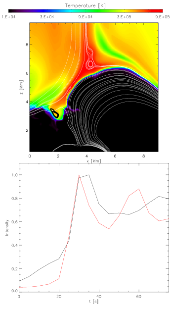
Figure 5: Top panel: Plasma temperature map of a snapshot of a 2D MHD model where a reconnection event occurs in the corona (Martínez-Sykora et al., 2012). The snapshot selected is at the peak Fe VIII emission, which is shown with the black contours around $[x,z]=[1.8,3.2]$ Mm. The magnetic field is shown with white lines. Bottom panel: Lightcurves of Fe VIII (red) and Fe X (black) emission averaged over an area corresponding to $3\times 3$ Hi-C pixels centered in the location where Fe VIII emission is strongest ($x=1.8$ Mm).

References

- Antiochos et al. (2003) Antiochos, S. K., Karpen, J. T., DeLuca, E. E., Golub, L., & Hamilton, P. 2003, ApJ, 590, 547
- Aulanier et al. (2007) Aulanier, G., et al. 2007, Science, 318, 1588
- Berger et al. (1999b) Berger, T. E., De Pontieu, B., Schrijver, C. J., & Title, A. M. 1999b, ApJ, 519, L97
- Boerner et al. (2012) Boerner, P., et al. 2012, Sol. Phys., 275, 41
- Bradshaw & Klimchuk (2011) Bradshaw, S. J., & Klimchuk, J. A. 2011, ApJS, 194, 26
- Brooks et al. (2009) Brooks, D. H., Warren, H. P., Williams, D. R., & Watanabe, T. 2009, ApJ, 705, 1522
- Brosius (2012) Brosius, J. W. 2012, ApJ, 754, 54
- Brosius & Holman (2012) Brosius, J. W., & Holman, G. D. 2012, A&A, 540, A24
- Cargill (1994) Cargill, P. J. 1994, ApJ, 422, 381
- Cargill & Klimchuk (1997) Cargill, P. J., & Klimchuk, J. A. 1997, ApJ, 478, 799
- Cassak & Drake (2009) Cassak, P. A., & Drake, J. F. 2009, ApJ, 707, L158
- Cirtain et al. (2013) Cirtain, J. J., Golub, L., Winebarger, A., & et al. 2013, Nature, 493, 501
- De Pontieu et al. (1999) De Pontieu, B., Berger, T. E., Schrijver, C. J., & Title, A. M. 1999, Sol. Phys., 190, 419
- De Pontieu et al. (2003a) De Pontieu, B., Erdélyi, R., & de Wijn, A. G. 2003a, ApJ, 595, L63
- De Pontieu et al. (2009) De Pontieu, B., Hansteen, V. H., McIntosh, S. W., & Patsourakos, S. 2009, ApJ, 702, 1016
- De Pontieu et al. (2011) De Pontieu, B., et al. 2011, Science, 331, 55
- De Pontieu et al. (2003b) De Pontieu, B., Tarbell, T., & Erdelyi, R. 2003b, ApJ, 590, 502
- Fletcher & De Pontieu (1999) Fletcher, L., & De Pontieu, B. 1999, ApJ, 520, L135
- Golub et al. (2007) Golub, L., et al. 2007, Sol. Phys., 243, 63
- Golub et al. (1990) Golub, L., Nystrom, G., Herant, M., Kalata, K., & Lovas, I. 1990, Nature, 344, 842
- Gudiksen et al. (2011) Gudiksen, B. V., Carlsson, M., Hansteen, V. H., Hayek, W., Leenaarts, J., & Martínez-Sykora, J. 2011, A&A, 531, A154
- Handy et al. (1999) Handy, B. N., et al. 1999, Sol. Phys., 187, 229
- Hansteen et al. (2010) Hansteen, V. H., Hara, H., De Pontieu, B., & Carlsson, M. 2010, ApJ, 718, 1070
- Kliem (1995) Kliem, B. 1995, in Lecture Notes in Physics, Berlin Springer Verlag, Vol. 444, Coronal Magnetic Energy Releases, ed. A. O. Benz & A. Krüger, 93
- Klimchuk (2006) Klimchuk, J. A. 2006, Sol. Phys., 234, 41
- Klimchuk et al. (2008) Klimchuk, J. A., Patsourakos, S., & Cargill, P. J. 2008, ApJ, 682, 1351
- Landi et al. (2013) Landi, E., Young, P. R., Dere, K. P., Del Zanna, G., & Mason, H. E. 2013, ApJ, 763, 86
- Lemen et al. (2012) Lemen, J. R., et al. 2012, Sol. Phys., 275, 17
- Martens et al. (2000) Martens, P. C. H., Kankelborg, C. C., & Berger, T. E. 2000, ApJ, 537, 471
- Martínez-Sykora et al. (2012) Martínez-Sykora, J., De Pontieu, B., & Hansteen, V. 2012, ApJ, 753, 161
- McTiernan (2009) McTiernan, J. M. 2009, ApJ, 697, 94
- Parker (1988) Parker, E. N. 1988, ApJ, 330, 474
- Peres et al. (1994) Peres, G., Reale, F., & Golub, L. 1994, ApJ, 422, 412
- Reale (2010) Reale, F. 2010, Living Reviews in Solar Physics, 7, 5
- Reale et al. (2011) Reale, F., Guarrasi, M., Testa, P., DeLuca, E. E., Peres, G., & Golub, L. 2011, ApJ, 736, L16
- Reale et al. (2009a) Reale, F., McTiernan, J. M., & Testa, P. 2009a, ApJ, 704, L58
- Reale & Orlando (2008) Reale, F., & Orlando, S. 2008, ApJ, 750, L10
- Reale et al. (2009b) Reale, F., Testa, P., Klimchuk, J. A., & Parenti, S. 2009b, ApJ, 698, 756
- Scherrer et al. (2012) Scherrer, P. H., et al. 2012, Sol. Phys., 275, 207
- Testa (2010) Testa, P. 2010, Space Sci. Rev., 130
- Testa et al. (2012) Testa, P., Drake, J. J., & Landi, E. 2012, ApJ, 745, 111
- Testa & Reale (2012) Testa, P., & Reale, F. 2012, ApJ, 750, L10
- Testa et al. (2011) Testa, P., Reale, F., Landi, E., DeLuca, E. E., & Kashyap, V. 2011, ApJ, 728, 30
- Tripathi et al. (2011) Tripathi, D., Klimchuk, J. A., & Mason, H. E. 2011, ApJ, 740, 111
- Tripathi et al. (2010) Tripathi, D., Mason, H. E., Del Zanna, G., & Young, P. R. 2010, A&A, 518, A42
- van Ballegooijen et al. (2011) van Ballegooijen, A. A., Asgari-Targhi, M., Cranmer, S. R., & DeLuca, E. E. 2011, ApJ, 736, 3
- Warren et al. (2011) Warren, H. P., Brooks, D. H., & Winebarger, A. R. 2011, ApJ, 734, 90
- Warren et al. (2012) Warren, H. P., Winebarger, A. R., & Brooks, D. H. 2012, ApJ, 759, 141
- Warren et al. (2008b) Warren, H. P., Winebarger, A. R., Mariska, J. T., Doschek, G. A., & Hara, H. 2008b, ApJ, 677, 1395
- Winebarger et al. (2011b) Winebarger, A. R., Schmelz, J. T., Warren, H. P., Saar, S. H., & Kashyap, V. L. 2008b, ApJ, 677, 1395