Scanning Gate Spectroscopy of transport across a Quantum Hall Nano-Island

Abstract

We explore transport across an ultra-small Quantum Hall Island (QHI) formed by closed quantum Hall edge states and connected to propagating edge channels through tunnel barriers. Scanning gate microscopy and scanning gate spectroscopy are used to first localize and then study a single QHI near a quantum point contact. The presence of Coulomb diamonds in the spectroscopy confirms that Coulomb blockade governs transport across the QHI. Varying the microscope tip bias as well as current bias across the device, we uncover the QHI discrete energy spectrum arising from electronic confinement and we extract estimates of the gradient of the confining potential and of the edge state velocity.

I Introduction

Most peculiar properties of quantum Hall systems stem from the propagation of electrons along one-dimensional edge channels, emerging wherever a Landau level crosses the Fermi energy Halperin_PRB1982 . The so-called Edge States (ES), that mainly form at the borders of a two-dimensional sheet of electrons in a high perpendicular magnetic field $B$, provide a powerful model that describes the behavior of quantum Hall nano-devices Buttiker_PRB1988 . Since scattering is topologically prohibited, ES offer a natural protection to electrons, so that they constitute ideal models of quantum wires, whose manipulation is particularly fruitful. Indeed, various device geometries can be carved from two-dimensional electron systems thanks to lithography techniques, and the position of ES within a device can then be tuned using voltages applied on metallic gates deposited on top of the device.

In this context, a strong interest recently emerged for interferometer geometries, where counterpropagating ES are brought close enough to interact, and electron loops can be formed at will. Tuning the coupling between ES leads to a large variety of situations. In open systems, i.e. when the conductance of the device $\sigma$ is much larger than $2e^{2}/h$, electronic analogs of Mach-Zehnder Ji_Nat2003 ; Neder_PRL2006 ; Roulleau_PRL2008 and Fabry-Pérot Rosenow_PRL2007 ; McClure_prl2009 ; Zhang_PRB09 ; Yamauchi_PRB09 ; Ofek_PNAS10 ; Halperin_PRB2011 interferometers allowed to study and control electron dephasing processes within ES and to estimate the electron phase coherence length Neder_PRL2006 ; Roulleau_PRL2008 ; Huynh_PRL_2012 . In particular, ref. McClure_prl2009 used interference checkerboard patterns generated in a Fabry-Pérot geometry to determine the edge state velocity in the quantum Hall regime. In the other extreme, $\sigma<<2e^{2}/h$, Quantum Hall Islands (QHIs) created by patterned quantum dots Altimiras_NatPhys09 or antidots Kataoka_prl1999 ; Sim_pr2008 ; Maasilta_PRB98 ; Michael_phE2006 ; Goldman_sc95 lead to the observation of a fractional electric charge  Goldman_sc95 ; Kou_prl2012 ; McClure_prl2012 and to the characterization of localized states’ confining potential Maasilta_PRB98 ; Sim_pr2008 ; Michael_phE2006 .

These pioneering experiments succeeded in evidencing electron interferences in model ES geometries, as well as signatures of charge tunneling through lithographically-patterned QHIs. Such phenomena can also occur in unpatterned two-dimensional electron systems: since the electron confining potential is never perfectly flat, electrons can be trapped in QHIs, pinned around potential ”hills” and ”dips”. The contribution of these QHIs to electron transport depends on their coupling to propagating ES. It is therefore important to devise methods to explore electron transport at the local scale in such systems, and new scanning probe techniques, derived from Atomic Force Microscopy (AFM) are now used for that purpose. The microscopic picture of electron localization was particularly investigated: compressibility measurements on quantum Hall localized states using a scanning single electron transistor revealed deviation from the single-particle picture Ilani_Nature2004 ; Martin_NatPhys2009 . Moreover, localized states as well as the electrostatic potential confining the two-dimensional electron systems could be imaged by monitoring the charging of a moving ‘bubble’ of electrons created in a two-dimensional electron system Finkelstein_Science2000 ; Steele_PRL2005 . Finally, Scanning Gate Microscopy (SGM) Topinka_Science2000 ; Crook_PRB2000 ; Kicin_NJP2005 ; Schnez_NJP2011 ; Hackens_NatPhys2006 ; MartinsPRL2007 ; PalaPRB2008 ; PalaNano2009 ; Kicin_PRB2004 ; Aoki_PRB2005 , directly relates the microscopic structure of a quantum Hall system to its transport properties. At the starting point of the present work is the discovery that SGM allows to precisely locate QHIs connected to propagating ES through tunnel barriers, and to decrypt the complex magnetoresistance oscillations patterns to which they give rise Hackens_NatComm2010 ; Paradiso_PRB2012 .

Here, we go beyond SGM and apply Scanning Gate Spectroscopy (SGS) Hackens_NatComm2010 ; Bleszynski-Jayich_prb2008 to access the discrete energy spectrum of an individual QHI pinned around a potential inhomogeneity. Unexpectedly, the QHI is located near one constriction of the quantum ring rather than around the central antidot. In SGS, the microscope tip is used as a local gate whose bias tunes the energy levels inside the QHI that is coupled to propagating ES by tunneling. Around filling factor $\nu$ = 6, the magnetoresistance of the quantum ring displays periodic oscillations. Thanks to SGM, we decrypt that they originate from Coulomb Blockade (CB) of electrons tunneling across a single ultra-small QHI. The CB interpretation is confirmed by the presence of Coulomb diamonds in the SGS spectrum. Importantly, lines parallel to the sides of Coulomb diamonds are associated with excited states arising from confinement. Using their energy spacing, we estimate the gradient of the confining potential and the associated edge state velocity around the QHI.

II Experimental setup and sample properties

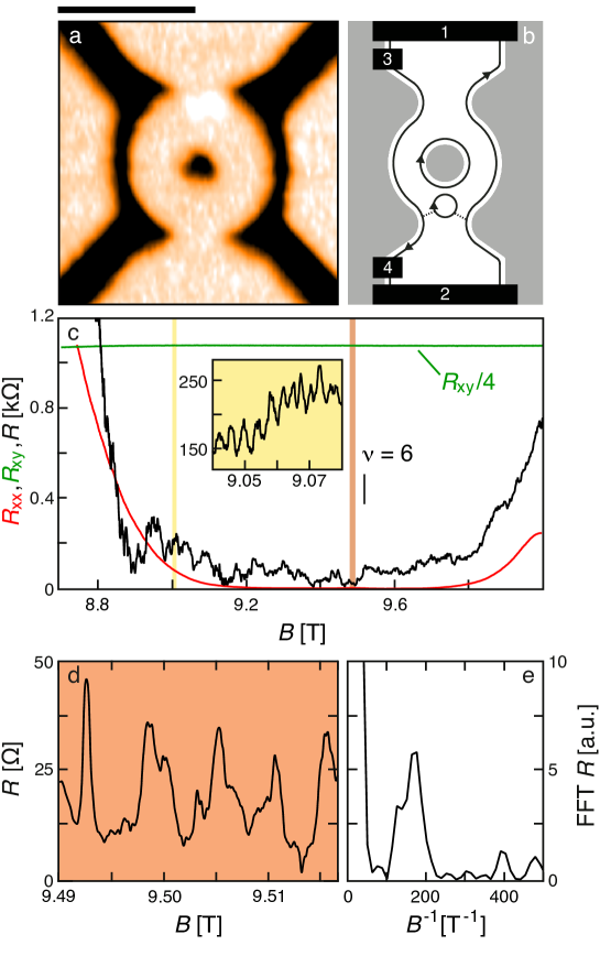
Figure 1: (Color online) (a) AFM topography of the quantum ring obtained at $B$ = 9.5 T and $T$ = 100 mK. The black bar represents 1 $\mu$m. (b) Schematic representation of our device showing a QHI connecting opposite edge channels through tunnel barriers (dotted lines). Current carrying contacts (1-2) and voltage probes (3-4) allow resistance measurements. (c) Magnetoresistance of the quantum ring ($R$) together with the longitudinal resistance $R_{\mathrm{xx}}$, in red, and the transverse resistance $R_{\mathrm{xy}}$, in green, of a Hall bar a next to $\nu~{}=~{}6$. In the inset we zoom a set periodic oscillations corresponding to the yellow region. (d) Close-up of the orange-shaded region in (c). (e) Fast Fourier transform of magnetoresistance (d).

Our experiments are carried out inside a ³He/⁴He dilution refrigerator at temperature $T$ = 100 mK. The cryostat is equipped with a superconducting coil that provides a magnetic field up to 15/17 T. A home made cryogenic AFM is attached at the bottom of the mixing chamber. The movement of the tip is detected via a piezoelectric tuning fork to which a conductive cantilever is glued Hackens_NatComm2010 . Using this setup, we perform measurements on a quantum ring patterned in an InGaAs/InAlAs heterostructure using e-beam lithography followed by wet etching. The two-dimensional electron gas is located 25 nm below the surface. In figure 1(a) we show an AFM topography of our device obtained at $B$ = 9.5 T and $T$ = 100 mK, just before SGM measurements.

As sketched in figure 1(b) the current is injected between ohmic contacts 1 and 2 and the voltage drop is measured between 3 and 4. Next to the ring, we patterned a Hall bar where we measure a low-$T$ electron density and mobility of $1.3\times 10^{16}~{}\mathrm{m^{-2}}$ and $4~{}\mathrm{m^{2}/Vs}$, respectively. Additionally, two lateral gates visible in figure 1(a) were grounded during the experiments shown here.

With the AFM tip connected to the ground, and retracted, around $\nu~{}=~{}6$ (measured in the Hall bar), the magnetoresistance of the device, shown in figure 1(c), displays oscillations with various periods which correspond to different QHIs being successively ”active” Hackens_NatComm2010 , i.e. tunnel-coupled to the propagating ES. A close up of a set of periodic oscillations is shown in the inset of figure 1(c). These magnetoresistance oscillations are not related to coherent electron interferences since their amplitude is inversely proportional to temperature which is consistent with pure Coulomb blockade Hackens_NatComm2010 . For the rest of our work, we focus on the orange-shaded region of figure 1(c), zoomed in figure 1(d), which displays periodic peaks with $\Delta B=$ 1/ 180 T $\sim$  5.6 mT as evidenced by the fast Fourier transform displayed in figure 1(e). This magnetic field range was chosen after reviewing the full trace and picking one region where the magnetoresistance was characterized by one dominant frequency, and where the resistance minima were the closest to zero so that the edge state picture, i.e. essentially no backscattering of edge states by the constriction, was the simplest. We understand these oscillations within a Coulomb-dominated model where electrons tunnel between propagating ES through a single QHI created around a potential inhomogeneity Rosenow_PRL2007 . Intuitively, this model states that a variation in the magnetic field creates an energy imbalance between the QHI and the propagating ES. This imbalance generates one CB-type oscillation per populated ES circling around the QHI per flux quantum $\phi_{\mathrm{0}}$. In this case, the device resistance oscillates with a period Rosenow_PRL2007 :

$$\Delta B=(\phi_{\mathrm{0}}/A)/N^{*},$$ (1)

where $N^{*}$ is the number of filled ES around the QHI and $A$ is the QHI area. From equation (1), figure 1(d), and assuming that $N^{*}=N=6$, where $N$ is the number of fully occupied ES in the bulk, we deduce that the QHI has a surface $A$ equivalent to that of a disk with a radius $r\simeq$ 200 nm.

III Imaging a QHI

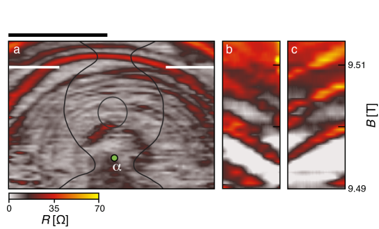
Figure 2: (Color online) (a) SGM map obtained at $B$ = 9.5 T, $T$ = 100 mK, $D_{\mathrm{tip}}=50$ nm and $V_{\mathrm{tip}}$ = 2 V. Continuous lines indicate the position of the quantum ring whereas $\alpha$ marks the origin of concentric fringes. The black bar represents 1 $\mu$m. (b-c) $B$-dependence of 500 nm long resistance profiles over the left/right regions marked with white lines in (a), respectively, with $V_{\mathrm{tip}}$ = -1 V.

We now use SGM in order to reveal the position of the active QHI by tuning the local potential landscape. It consists in scanning the polarized tip ($V_{\mathrm{tip}}$) along a plane parallel to the two-dimensional electron system at a distance $D_{\mathrm{tip}}=50$ nm, which roughly corresponds to the lateral extent of the tip-induced potential full width at half maximum Gildemeister_PRB2007 , while recording, at every point, the resistance of the device. figure 2(a) shows a SGM map recorded at $B$ = 9.5 T, $V_{\mathrm{tip}}$ = 2 V and $T$ = 100 mK. The continuous black lines superimposed on the image indicate the lithographic edges of the quantum ring. Concentric fringes decorate the SGM map and their center indicates the position of the active QHI (point $\alpha$ in figure 2(a)). Indeed, approaching the polarized tip modifies the potential on the island. It therefore gradually changes its area $A$ and hence the magnetic flux $\phi$ enclosed by circling ES. Equivalently to the effect of $B$ described above, varying the tip-QHI distance also generates CB-type oscillations and isoresistance lines on figure 2(a) are indeed iso-$\phi$ lines. Variations of the visibility of the fringes are observed when the tip approaches the QHI, a typical feature of CB experiments Kouwenhoven_AS1997 ; BennekerPRB1991 . Furthermore, the amplitude also varies along a single concentric fringe, most likely due to the variation of the tunneling strength through the QHI, which depends sharply on the potential landscape. In figure 2(a), we chose $V_{\mathrm{tip}}$ = 2 V to make sure that $N^{*}=N=6$ during the entire scan. Otherwise, when approaching a negatively charged tip near the constrictions of the quantum ring, $N^{*}$ decreases and the resistance sharply increases Aoki_PRB2005 , which hinders the observation of CB-type fringes. Noteworthy, the same fringes are present in both negative and positive $V_{\mathrm{tip}}$ as long as $N^{*}=N$, i.e. for both repulsive or attractive tip potential, respectively. Changing $V_{\mathrm{tip}}$, the fringes are simply shifted with respect to the position of the QHI.

The effects of both $B$ and tip-QHI distance along the white lines in the left and right sides of figure 2(a) are illustrated in figures 2(b) and (c), respectively (note that figure 2(a) was obtained with positive $V_{\mathrm{tip}}$ while figure 2(b) and (c) with negative $V_{\mathrm{tip}}$). Along the $B$-axis, clear oscillations are visible with a period around $\Delta B\sim 6$ mT in agreement with the magnetoresistance in figure 1(d). For the case of a potential hill, resistance peaks should follow positive $dV_{\mathrm{tip}}/dB$ slopes, i.e. decreasing $B$ should be compensated by a tip voltage decrease in order to keep the same magnetic flux through the QHI Zhang_PRB09 ; Ofek_PNAS10 ; Halperin_PRB2011 . In our case, approaching the negatively charged tip has the same effect as decreasing $V_{\mathrm{tip}}$ as it corresponds to an increase of the QHI area. The slope of the fringes in figures 2(b-c) therefore supports the CB picture.

Finally, the ES model states that a complete reflection of $K$ edge channels by a quantum point contact gives rise to a resistance shift of $\frac{h}{e^{2}}\left(\frac{1}{N-K}-\frac{1}{N}\right)$ Aoki_PRB2005 ; Buttiker_PRB1988 . Using this argument Buttiker_PRB1988 with $N$ = 6 and taking into account that the amplitude of the oscillations is around $40\Omega$, we deduce $K$ = 0.05, meaning that the peak conductance across the QHI is about 0.05 $e^{2}/h$, also consistent with the tunneling regime required for CB. This also means that most of the current flows in the transmitted ES and only a small fraction is used to probe the QHI, in contrast with typical CB experiments where all the current flows through the quantum dot.

IV Local spectroscopy of the QHI

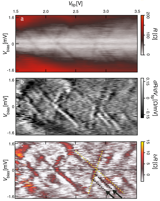
Figure 3: (Color online) (a) SGS measured when placing the tip at $\alpha$, in figure 2(a). (b) Numerical derivative $dR/dV_{\mathrm{tip}}$ of (a) in the $V_{\mathrm{tip}}-V_{\mathrm{bias}}$ plane. Note that each resonance in the differential resistance appears as a black and white double line. (c) High-pass-filter version of (a), where two yellow dashed lines indicate the transition between Coulomb-blockaded regions. Black dashed lines highlight Coulomb excited states.

A deeper understanding of the QHI’s electronic structure can be reached using SGS: positioning the tip at point $\alpha$, both $V_{\mathrm{tip}}$ and the current $I$ through the device are swept. The bias current can be converted to a voltage bias $V_{\mathrm{bias}}$ across the QHI thanks to the quantized Hall resistance: $V_{\mathrm{bias}}=h/(e^{2}N)I$. The plot of the differential resistance $R$ in the ($V_{\mathrm{tip}}$, $V_{\mathrm{bias}}$) plane is drawn in figure 3(a), where a set of narrow straight lines is superimposed on a slowly-varying background. We associate this background to the breakdown of the QH regime as a large current flows through the device Nachtwei_PhyE1999 . Straight lines are more apparent in figure 3(b), where the numerical derivative $dR/dV_{\mathrm{tip}}$ of figure 3(a) is plotted, as well as in figure 3(c), where a smooth background was subtracted from the raw $R$ vs $[V_{\mathrm{tip}},V_{\mathrm{bias}}]$ data to obtain $\delta R$. Consistently with previous observations, crossing lines (two of them are highlighted with yellow dashed lines) correspond to transitions between Coulomb blockaded regions as energy levels of the QHI enter in the bias window defined by the source and drain electro-chemical potentials. The slopes are determined by the various capacitances $C_{\Sigma}$ of the system. Crossing lines form Coulomb diamonds analog to those measured in closed quantum dots at $B$ = 0 T Kouwenhoven_AS1997 .

Parallel to the borders of the Coulomb diamonds, additional lines are visible, highlighted with black dashed lines in figure 3(c). Noteworthy, these lines do not enter the adjacent Coulomb diamond, a characteristic signature of excited states Reimann_RMP_2002 . The energy gap between these excited states is $\Delta E\simeq$ 380 $\mu$eV, much smaller than the Landau level spacing, $\Delta E_{\mathrm{LL}}\simeq 26.8$ meV, and the Zeeman splitting, $\Delta E_{\mathrm{z}}\simeq 1.65$ meV, in our system around $B=9.5$ T. These values are determined making use of $\Delta E_{\mathrm{LL}}=\hbar eB/m^{*}$, where $e$ is the electron charge, $m^{*}=0.041~{}m_{\mathrm{e}}$ is the electron effective mass in our two-dimensional electron system with respect to the free electron mass $m_{\mathrm{e}}$ Kotera_PhysE2001 , and $\Delta E_{\mathrm{z}}=|g|\mu_{\mathrm{\beta}}B$, where $\mu_{\mathrm{\beta}}$ is the Bohr magneton and $g\simeq 3$ is the Landé g-factor in the heterostructure Nitta_APL2003 . The QHI is thus in the quantum limit of CB defined by $k_{B}T<<\Delta E<<e^{2}/C_{\Sigma}\sim 1.6$ meV obtained from figure 3(b) Kouwenhoven_AS1997 , which justifies the $1/T$ temperature dependence found previously in Hackens_NatComm2010 . Assuming that the Coulomb excited states emerge as a consequence of circular confinement, we can determine an average of the derivative of the confining potential $dU/dr$ using the relation Kataoka_prl1999 ; Sim_pr2008 ; Michael_phE2006 :

$$\Delta E=\hbar v/r=|dU/dr|\hbar/(e~{}rB),$$ (2)

where $v$ is the ES velocity in the QHI. Taking into account that $r\simeq$ 200 nm, we obtain $|dU/dr|\simeq$ 1 meV/nm for the QHI formed around a potential inhomogeneity. In QHIs created around antidots etched in GaAs/AlGaAs heterostructures Kataoka_prl1999 ; Maasilta_PRB98 ; Michael_phE2006 , which are known to generate soft-wall potentials, $|dU/dr|$ was found to be around 20 $\mu$eV/nm Maasilta_PRB98 , and data in Kataoka_prl1999 ; Michael_phE2006 give $|dU/dr|\simeq$ 50 $\mu$eV/nm. In the case of a GaAs quantum Hall Fabri-Pérot interferometer McClure_prl2009 , in the high-magnetic-field limit, $|dU/dr|$ was found to be 80 $\mu$eV/nm. These results are summarized in table (1), from which we conclude that $|dU/dr|$ scales with the carrier density of the two-dimensional electron system Eksi _prb2007 : $1\times 10^{15}~{}\mathrm{m^{-2}}$ Maasilta_PRB98 , $2.6\times 10^{15}~{}\mathrm{m^{-2}}$ Kataoka_prl1999 ; Michael_phE2006 , $2.7\times 10^{15}~{}\mathrm{m^{-2}}$ McClure_prl2009 and $1.4\times 10^{16}~{}\mathrm{m^{-2}}$ in the present sample. In the same framework, using equation (2), we extract $v=9.8\times 10^{4}$ m/s, which is close to the lower limit of results in McClure_prl2009 . As $v$ decreases with increasing $B$, this data copes with the larger values reported in McClure_prl2009 at lower $B$. The numerical values determined here for $v$ and $|dU/dr|$ constitute upper bounds as the shape of the QHI is assumed to be circular.

Reference	Carrier density (${m^{-2}}$)	$|dU/dr|$ ($\mu$eV/nm)
Maasilta_PRB98	$1\times 10^{15}$	20
Kataoka_prl1999 ; Michael_phE2006	$2.6\times 10^{15}$	50
McClure_prl2009	$2.7\times 10^{15}$	80
this work	$1.4\times 10^{16}$	1000

Table 1: Comparison between $dU/dr$ calculated from data in the literature and extracted in this work as a function of the carrier density in the 2DES.

V Conclusion

In conclusion, we have used SGM to locate an individual quantum Hall island and directly probed its excited states arising from confinement with SGS. We were able to confirm that Coulomb blockade governs transport and to characterize the confining potential of the QHI. Both the slope of the confining potential and the edge state velocity were estimated. The combination of SGM and SGS techniques is therefore extremely useful to unveil the microscopic nature of charge transport inside complex nanodevices even in the quantum Hall regime, just like the combination of scanning tunneling microscopy and scanning tunneling spectroscopy was key to understand the electronic local density of states of surface nanostructures. Another advantage of the presence of the tip is the possibility to tune in situ the local electrostatic environment of the nano-device by depositing charges on its surface Crook _Nature2003 . This way, one could envision to induce QHIs with controlled geometries.

References

- (1) Halperin B I 1982 Phys. Rev. B 25 2185
- (2) Büttiker M 1988 Phys. Rev. B 38 9375
- (3) Ji Y,Chung Y C, Sprinzak D, Heiblum M, Mahalu D and Shtrikman H 2003 Nature 422 415
- (4) Neder I, Heiblum M, Levinson Y, Mahalu D and Umansky V 2006 Phys. Rev. Lett. 96 016804
- (5) Roulleau P, Portier F, Roche P, Cavanna A, Faini G, Gennser U and Mailly D 2008 Phys. Rev. Lett. 100 126802
- (6) Rosenow B and Halperin B I 2007 Phys. Rev. Lett. 98 106801
- (7) McClure D T, Zhang Y, Rosenow B, Levenson-Falk E M, Marcus C M, Pfeiffer L N and West K W 2009 Phys. Rev. Lett. 103 206806
- (8) Zhang Y, McClure D T, Levenson-Falk E M, Marcus C M, Pfeiffer L N and West K W 2009 Phys. Rev. B 79 241304
- (9) Yamauchi Y, Hashisaka M, Nakamura S, Chida K, Kasai S, Ono T, Leturcq R, Ensslin K, Driscoll D C, Gossard A C and Kobayashi K 2009 Phys. Rev. B 79 161306
- (10) Ofek N, Bid A, Heiblum M, Stern A, Umansky V and Mahalu D 2010 Proc. Nat. Acad. Sci. 107 5276
- (11) Halperin B, Stern A, Neder I and Rosenow B 2011 Phys. Rev. B 83 155440
- (12) Huynh P-A, Portier F, le Sueur H, Faini G, Gennser U, Mailly D, Pierre F, Wegscheider W and Roche P 2012 Phys. Rev. Lett. 108 256802
- (13) Altimiras C, le Sueur H, Gennser U, Cavanna A,Mailly D and Pierre F, 2009 Nature Phys. 6 34
- (14) Kataoka M, Ford C J B, Faini G, Mailly D, Simmons M Y, Mace D R, Liang C -T and Ritchie D A 1999 Phys. Rev. Lett. 83 160
- (15) Sim H -S, Kataoka M and Ford C J B 2008 Phys. Rep. 456 127
- (16) Maasilta I J and Goldman V J 1998 Phys. Rev. B 57 R4273
- (17) Michael C P, Kataoka M, Ford C J B, Faini G, Mailly D, Simmons M Y and Ritchie D A 2006 Physica E 34 195
- (18) Goldman V J and Su B 1995 Science 267 1010
- (19) Kou A, Marcus C M, Pfeiffer L N and West K W 2012 Phys. Rev. Lett. 108 256803
- (20) McClure D T, Chang W, Marcus C M, Pfeiffer L N and West K W 2012 Phys. Rev. Lett. 108 256804
- (21) Ilani S, Martin J, Teitelbaum E, Smet J H, Mahalu D, Umansky V and Yacoby A 2004 Nature 427 328
- (22) Martin J, Akerman N, Ulbricht G, Lohmann T, von Klitzing K, Smet J H and Yacoby A 2009 Nature Phys. 5 669-674
- (23) Finkelstein G, Glicofridis P I, Ashoori R C and Shayegan M 2000 Science 289 90
- (24) Steele G A, Ashoori R C, Pfeiffer L N and West K W 2005 Phys. Rev. Lett. 95 136804
- (25) Topinka M A, LeRoy B J, Shaw S E J, Heller E J, Westervelt R M, Maranowski K D and Gossard A C 2000 Science 289 2323
- (26) Crook R, Smith C G, Simmons M Y and Ritchie D A 2000 Phys. Rev. B 62 5174
- (27) Kic̆in S, Pioda A, Ihn T, Sigrist M, Fuhrer A, Ensslin K, Reinwald M and Wegscheider W 2005 New J. Phys. 7 185
- (28) Schnez S, G ttinger J, Stampfer C, Ensslin K and Ihn T 2011 New J. Phys. 13 053013
- (29) Hackens B, Martins F, Ouisse T, Sellier H, Bollaert S, Wallart X, Cappy A, Chevrier J, Bayot V and Huant S 2006 Nature Phys. 2 826
- (30) Martins F, Hackens B, Pala M G, Ouisse T, Sellier H, Wallart X, Bollaert S, Cappy A, Chevrier J, Bayot V and Huant S 2007 Phys. Rev. Lett. 99 136807
- (31) Pala M G, Hackens B, Martins F, Sellier H, Bayot V, Huant S and Ouisse T 2008 Phys. Rev. B 77 125310
- (32) Pala M G, Baltazar S, Martins F, Hackens B, Sellier H, Ouisse T, Bayot V and Huant S 2009 Nanotechnology 20 264021
- (33) Kic̆in S, Pioda A, Ihn T, Ensslin K, Driscoll D C and Gossard A C 2004 Phys. Rev. B 70 205302
- (34) Aoki N, da Cunha C R, Akis R, Ferry D K and Ochiai Y 2005 Phys. Rev. B 72 155327
- (35) Hackens B, Martins F, Faniel S, Dutu C A, Sellier H, Huant S, Pala M, Desplanque L, Wallart X and Bayot V 2010 Nature Comm 1 39
- (36) Paradiso N, Heun S, Roddaro S, Biasiol G, Sorba L, Venturelli D, Taddei F, Giovannetti V, and Beltram F 2012 Phys. Rev. B 86 085326
- (37) Bleszynski-Jayich A C, Froberg L E, Bjork M T, Trodahl H J, Samuelson L and Westervelt R M 2008 Phys. Rev. B 77 245327
- (38) Gildemeister A E, Ihn T, Sigrist M, Ensslin K, Driscoll D C and Gossard A C 2007 Phys. Rev. B 75 195338
- (39) Kouwenhoven L P, Marcus C M, McEuen P L, Tarucha S, Westervelt R M and Wingreen N S 1997 in Series E: Applied Sciences (eds Sohn L L, Kouwenhoven L P and Schon G) 345 105214 (Kluwer Academic)
- (40) Beenakker C W J 1991 Phys. Rev. B 44 1646
- (41) Nachtwei G 1999 Physica E 4 79
- (42) Hanson R, Kouwenhoven L P, Petta J R, Tarucha S and Vandersypen L M K 2007 Rev. Mod. Phys. 79 1217-1265
- (43) Kotera N, Arimoto H, Miura N, Shibata K, Ueki Y, Tanaka K, Nakamura H, Mishima T, Aiki K and Washima M 2001 Physica E 11 219 223
- (44) Nitta J, Lin Y P, Akazaki T and Koga T 2003 Appl. Phys. Lett. 22 4565-4567
- (45) Eksi D, Cicek E, Mese A I, Aktas S, Siddiki A and Hakioğlu T 2007 Phys. Rev. B 76 075334
- (46) Crook R, Graham A C, Smith C G, Farrer I, Beere H E and Ritchie D A 2003 Nature 424 751