Quintom potentials from quantum cosmology using the FRW cosmological model

Abstract

We construct the quintom potential of dark energy models in the framework of spatially flat Friedmann-Robertson Walker universe in the inflationary epoch, using the Bohm like approach, known as amplitude-real-phase. We find some potentials for which the wave function of the universe is found analytically and we have obtained the classical trajectories in the inflation era.

I Introduction

At the present time, there are some efforts to explain the observations for the accelerated expansion of the universe, based on the dynamics of a scalar (quintessence) or multiscalar field (quintom) as models for dark energy, (see the review (Copeland et al.,, 2006; Feng,, 2006; Cai et al.,, 2010)). The properties of the quintom models have been studied from different points of view. Among them, the phase space studies, using the dynamical systems tools, are very useful in order to analyze the qualitative and asymptotic behavior of the model (Guo,, 2005; Feng,, 2005; Sadjadi,, 2006; Guo,, 2006; Feng,, 2006; Zhao,, 2006; Cai, 2007a, ; Cai, 2007b, ; Alimohammadi,, 2007; Lazkoz,, 2007; Cai, 2008a, ; Cai, 2008b, ; Zhang,, 2008; Sadeghi,, 2008; Nozari,, 2009; Setare,, 2009; Setare et al.,, 2009; Sadeghi,, 2009; Qiu,, 2010; Saridakis, 2010a, ; Amani,, 2011; Farajollahi,, 2012)). In the present work we want to investigate the case of quintom cosmology constructed by using both quintessence ($\sigma$) and phantom ($\phi$) fields, maintaining a nonspecific potential $\rm V(\phi,\sigma)$ from the begining. In the literature one special class of potential used is the sum of the exponential potentials for each field (Guo,, 2005; Sadjadi,, 2006; song et al.,, 2005; Zhao,, 2006; Chimento,, 2009). There are other works where other type of potentials are analyzed Copeland et al., (2006); Zhao, (2006); Setare et al., (2009); Cai, 2008b ; Adak et al., (2011); Setare, (2009); Saridakis, 2010a ; Amani, (2011).

We claim that the analysis of general potentials using dynamical systems was made considering particular structures of them, in other words, how can we introduce this mathematical structure within a physical context? We can partially answer this question, when the amplitude-real-phase formalism is introduced, in the sense that, some potentials can be constructed (Guzmán et al.,, 2007; J. Socorro et al.,, 2010; Bohm,, 1952).

This work is arranged as follows. In section II we present the corresponding Einstein-Klein-Gordon equation for the quintom model. Also we introduced the hamiltonian apparatus which is applied to FRW cosmological model in order to construct a master equation for barotropic perfect fluid and cosmological constant. Furthermore, we present the classical equations for the flat FRW, which are presented in section V for particular scalar potentials. In subsection III we present the quantum scheme, where we will use the amplitude-real-phase ansatz in order to solve the WDW equation. This method was used by Moncrief and Ryan Moncrief & Ryan, (1991) to obtain exact solutions for the Bianchi type IX anisotropic cosmological model with a wavefunction of the form $\rm\Psi=We^{-S}$. This form of the wavefunction was motivated by the work of Kodama Kodama, (1988, 1990). Our treatment is applied to build the mathematical structure of quintom scalar potentials which allow us obtain exact solutions together with an arbitrary factorization of the WDW equation. In this work we have obtain the wave function of the universe in order to find the quantum potentials, which is a more important matter in order to find the classical trajectories, which is shown in section V, that is devoted to obtain the classical solutions for particular scalar potentials, also we show graphically the classical trajectory in the configuration space $\rm(\Omega,\varphi)$ projected from its quantum counterpart. In this same section, we present the time dependence for the $\Omega$, and quintom scalar fields ($\varphi\,,\varsigma$) for the potentials treated in this section. In section VI is devoted to final remarks of this work.

II The Quintom model

We begin with the construction of the quintom cosmological theory, which requires the simultaneous consideration of two fields, namely, a canonical one $\sigma$, and phantom one $\phi$ (see equation (12) below and reference Setare et al., (2009)). The lagrangian density of this theory with two fields, the cosmological term, and matter contribution, is

$$\rm{\cal L}=\sqrt{-g}\left(R-2\Lambda-\frac{1}{2}g^{\mu\nu}\nabla_{\mu}\phi\nabla_{\nu}\phi+\frac{1}{2}g^{\mu\nu}\nabla_{\mu}\sigma\nabla_{\nu}\sigma-V(\phi,\sigma)\right)+{\cal L}_{matter},$$ (1)

the corresponding field equations for perfect fluid matter content are

$$\rm G_{\alpha\beta}+g_{\alpha\beta}\Lambda = \rm-\frac{1}{2}\left(\nabla_{\alpha}\phi\nabla_{\beta}\phi-\frac{1}{2}g_{\alpha\beta}g^{\mu\nu}\nabla_{\mu}\phi\nabla_{\nu}\phi\right)+\frac{1}{2}\left(\nabla_{\alpha}\sigma\nabla_{\beta}\sigma-\frac{1}{2}g_{\alpha\beta}g^{\mu\nu}\nabla_{\mu}\sigma\nabla_{\nu}\sigma\right)$$ (2)

$$\rm-\frac{1}{2}g_{\alpha\beta}\,V(\phi,\sigma)-8\pi GT_{\alpha\beta},$$

$$\rm g^{\mu\nu}\phi_{,\mu\nu}-g^{\alpha\beta}\Gamma^{\nu}_{\alpha\beta}\nabla_{\nu}\phi+\frac{\partial V}{\partial\phi} = \rm 0,\qquad\Leftrightarrow\quad\Box\phi+\frac{\partial V}{\partial\phi}=0$$

$$\rm g^{\mu\nu}\sigma_{,\mu\nu}-g^{\alpha\beta}\Gamma^{\nu}_{\alpha\beta}\nabla_{\nu}\sigma-\frac{\partial V}{\partial\sigma} = \rm 0,\qquad\Leftrightarrow\quad\Box\sigma-\frac{\partial V}{\partial\sigma}=0,$$

$$\rm T^{\mu\nu}_{\,\,;\mu} = \rm 0,\quad with\quad T_{\mu\nu}=Pg_{\mu\nu}+(P+\rho)u_{\mu}u_{\nu},$$ (3)

here $\rho$ is the energy density, P the pressure, and $\rm u_{\mu}$ the velocity of the fluid, satisfying that $\rm u_{\mu}u^{\mu}=-1$.

Let us recall here the canonical formulation in the ADM formalism for flat FRW cosmological model. The metric has the form

$$\rm ds^{2}=-N(t)dt^{2}+e^{2\Omega(t)}\left[dr^{2}+r^{2}\left(d\theta^{2}+\sin^{2}\theta d\phi^{2}\right)\right],$$ (4)

where the scale factor is defined as $\rm A=e^{\Omega(t)}$, where $\rm\Omega\epsilon\,(-\infty,\infty)$.

The lagrangian density (1) for FRW cosmological model is written as

$$\rm{\cal L}_{FRW}=\rm e^{3\Omega}\left[6\frac{\dot{\Omega}^{2}}{N}+6\frac{\dot{\varphi}^{2}}{N}-6\frac{\dot{\varsigma}^{2}}{N}+N\left(-V(\varphi,\varsigma)+2\Lambda+16\pi G\rho\right)\right],$$ (5)

where the overdot denotes time derivative, the fields were re-scaled as $\phi=\sqrt{12}\varphi,\sigma=\sqrt{12}\varsigma$ for simplicity in the calculations.

The momenta are define in the usual way, $\rm\Pi_{q^{i}}=\rm\frac{\partial{\cal L}}{\partial\dot{q}^{i}}$, where $\rm q^{i}=(A,\varphi,\varsigma)$ are the fields coordinates of the model.

$$\rm\Pi_{\Omega} = \rm\frac{\partial{\cal L}}{\partial\dot{\Omega}}=\frac{12e^{3\Omega}\dot{\Omega}}{N},\qquad\to\dot{\Omega}=\frac{N\Pi_{\Omega}}{12}e^{-3\Omega}$$

$$\rm\Pi_{\varphi} = \rm\frac{\partial{\cal L}}{\partial\dot{\varphi}}=12\frac{e^{3\Omega}\dot{\varphi}}{N},\qquad\to\dot{{\varphi}}=+\frac{N\Pi_{\varphi}}{12}e^{-3\Omega}$$

$$\rm\Pi_{\varsigma} = \rm\frac{\partial{\cal L}}{\partial\dot{\varsigma}}=-12\frac{e^{3\Omega}\dot{\varsigma}}{N},\qquad\to\dot{{\varsigma}}=-\frac{N\Pi_{\varsigma}}{12}e^{-3\Omega}.$$ (6)

Writing (5) in the canonical form, $\rm{\cal L}_{canonical}=\Pi_{q}\dot{q}-N{\cal H}$ and substituting the energy density of the barotropic fluid $\rm P=\gamma\rho$, which was found using the covariant derivative of the energy-momentum tensor (3), $\rm\rho=M_{\gamma}e^{-3\left(1+\gamma\right)\Omega},$ where $M_{\gamma}$ is an integration constant. The corresponding Hamiltonian density ${\cal H}$ considering in this work the inflationary epoch, that corresponds to the value $\gamma=-1$, becomes

$$\rm{\cal H}_{FRW}=\frac{e^{-3\Omega}}{24}\left[\Pi_{\Omega}^{2}-\Pi_{\varsigma}^{2}+\Pi_{\varphi}^{2}+e^{6\Omega}\left\{24V(\varphi,\varsigma)-\lambda_{eff}\right\}\right],$$ (7)

where $\rm\lambda_{eff}=48(\Lambda+8\pi GM_{{}_{-1}})$.

The Einstein field equations (2,3) for the flat FRW cosmological model with barotropic state equation, are

$$\rm 3\frac{\dot{\Omega}^{2}}{N^{2}} = \rm 8\pi G\rho-3\frac{\dot{\varphi}^{2}}{N^{2}}+3\frac{\dot{\varsigma}^{2}}{N^{2}}+\Lambda+\frac{V(\varphi,\varsigma)}{2},$$ (8)

$$\rm 2\frac{\ddot{\Omega}}{N^{2}}+3\frac{\dot{\Omega}^{2}}{N^{2}}-2\frac{\dot{\Omega}\dot{N}}{N^{3}} = \rm-8\pi GP+3\frac{\dot{\varphi}^{2}}{N^{2}}-3\frac{\dot{\varsigma}^{2}}{N^{2}}+\Lambda+\frac{V(\varphi,\varsigma)}{2},$$ (9)

$$\rm-3\frac{\dot{\Omega}\dot{\varsigma}}{N^{2}}+\frac{\dot{N}\dot{\varsigma}}{N^{3}}-\frac{\ddot{\varsigma}}{N^{2}}+\frac{\partial V(\varsigma,\varphi)}{\partial\varsigma} = 0,$$ (10)

$$\rm-3\frac{\dot{\Omega}\dot{\varphi}}{N^{2}}+\frac{\dot{N}\dot{\varphi}}{N^{3}}-\frac{\ddot{\varphi}}{N^{2}}-\frac{\partial V(\varsigma,\varphi)}{\partial\varphi} = 0,$$ (11)

which can be written as

$$\rm 8\pi G\rho+\Lambda+\frac{1}{2}\left(-6\varphi^{\prime 2}+6\varsigma^{\prime 2}+V(\varphi,\varsigma)\right) = \rm 3H^{2},$$ (12)

$$\rm 8\pi GP-\Lambda+\frac{1}{2}\left(-6\varphi^{\prime 2}+6\varsigma^{\prime 2}-V(\varphi,\varsigma)\right)=-2\Omega^{\prime\prime}-3H^{2} = \rm 3H^{2}q-H^{2},$$ (13)

$$\rm-3\Omega^{\prime}\varsigma^{\prime}-\varsigma^{\prime\prime}+\frac{\partial V(\varsigma,\varphi)}{\partial\varsigma} = 0,$$ (14)

$$\rm-3\Omega^{\prime}\varphi^{\prime}-\varphi^{\prime\prime}-\frac{\partial V(\varsigma,\varphi)}{\partial\varphi} = 0,$$ (15)

where the Hubble parameter is define as $\rm H=\frac{\dot{A}}{A}=\dot{\Omega}$ and the deceleration parameter $q=-\frac{A\ddot{A}}{\dot{A}^{2}}$. We have done the time transformation $\rm\frac{d}{d\tau}=\frac{d}{Ndt}=\prime$.

Adding (12) and (13) we obtain

$$\rm-\Omega^{\prime\prime}=4\pi G\left[\rho+\rho_{\varphi}+\rho_{\varsigma}+P+P_{\varphi}+P_{\varsigma}\right],$$ (16)

where

$$\rm P_{\varphi} = \rm\frac{1}{16\pi G}\left(-6\varphi^{\prime 2}-V(\varphi,\varsigma)|_{\varsigma}\right),\qquad P_{\varsigma}=\frac{1}{16\pi G}\left(6\varsigma^{\prime 2}-V(\varphi,\varsigma)|_{\varphi}\right),$$

$$\rm\rho_{\varphi} = \rm\frac{1}{16\pi G}\left(-6\varphi^{\prime 2}+V(\varphi,\varsigma)|_{\varsigma}\right),\qquad\rho_{\varsigma}=\frac{1}{16\pi G}\left(6\varsigma^{\prime 2}+V(\varphi,\varsigma)|_{\varphi}\right),$$

which are useful when we study the behavior of dynamical systems. Additionally we can introduce the total quintom energy density and pressure as:

$$\rho_{{}_{DE}}=\rho_{\varsigma}+\rho_{\varphi},\qquad P_{{}_{DE}}=P_{\varsigma}+P_{\varphi},\qquad P_{{}_{DE}}=\omega_{{}_{DE}}\rho_{{}_{DE}}$$ (17)

where

$$\rm\omega_{{}_{DE}}=\frac{6\varsigma^{\prime 2}-6\varphi^{\prime 2}-V(\varsigma,\varphi)}{6\varsigma^{\prime 2}-6\varphi^{\prime 2}+V(\varsigma,\varphi)}=-1-\frac{12\left(\varphi^{\prime 2}-\varsigma^{\prime 2}\right)}{V(\varsigma,\varphi)-6\left(\varphi^{\prime 2}-\varsigma^{\prime 2}\right)}.$$ (18)

For phenomenological analysis, (18) will serve us as a test for the viable class of quintom potentials whose equation of state can cross the cosmological constant barrier which $\omega_{{}_{DE}}=-1$ is mildly favored of observations Melchiorri, et al. (2002). For instance, when $\rm V(\varsigma,\varphi)>0$ and $\rm V(\varsigma,\varphi)>6\varphi^{\prime 2}-6\varsigma^{\prime 2}$, then the kinetic terms satisfies $\rm\varsigma^{\prime 2}<\varphi^{\prime 2}$, so, the barotropic parameter $\rm\omega_{{}_{DE}}<-1$. In this case, the intensity of the phantom field $\rm\varphi$ always is larger than the intensity of the quintessence field $\rm\varsigma$. In other case, we have that $\rm\omega_{{}_{DE}}>-1$. The particular value equivalent to cosmological constant is when the kinetic terms are null or equal in both fields.

For constant potential, equations (14,15) can be solved in terms of the $\Omega$ function,

$$\rm\varsigma^{\prime} = \rm\varsigma_{0}e^{-3\Omega},\qquad\varsigma(\tau)=\varsigma_{0}\int e^{-3\Omega(\tau)}d\tau+\varsigma_{1},$$ (19)

$$\rm\varphi^{\prime} = \rm\varphi_{0}e^{-3\Omega},\qquad\varphi(\tau)=\varphi_{0}\int e^{-3\Omega(\tau)}d\tau+\varphi_{1},$$ (20)

We obtain in implicit solution for $\Omega$ in a quadrature

$$\rm\int\frac{d\Omega}{\sqrt{F(\Omega)}}=\Delta\tau,$$ (21)

where $\rm F(\Omega)$ is given by

$$\rm F(\Omega)=\frac{8\pi GM_{\gamma}}{3}e^{-3(1+\gamma)\Omega}+\left(-\varphi_{0}^{2}+\varsigma_{0}^{2}\right)e^{-6\Delta\Omega}+\frac{\Lambda_{eff}}{3},$$

with $\rm\Lambda_{eff}=\Lambda+V_{0}/2.$ For particular values of the parameter $\gamma$, has analytical solution.

For one scalar field, with constant potential, the formalism is like the one formulated by Sáez and Ballester in 1986, because both field are equivalent, see equations (14,15) Sáez & Ballester, (1986). This formalism was studied by one of the author and collaborators, in the FRW and Bianchi type Class A cosmological models, J. Socorro et al., (2010); M. Sabido et al., (2010); J. Socorro et al., (2011).

III quantum cosmology

The Wheeler-DeWitt equation for this model is obtained introducing the representation (we choose $\hbar=1$) $\rm\Pi_{q^{\mu}}=-i\partial_{q^{\mu}}$ into (7). The factor $\rm e^{-3\Omega}$ can be ordered with the momenta $\rm\hat{\Pi}_{\Omega}$ in many ways. Hartle and Hawking (Hartle & Hawking,, 1983) have suggested a semi-general factor ordering for $\rm e^{-3\Omega}\hat{\Pi}^{2}_{\Omega}$ as

$$\rm-e^{-(3-Q)\Omega}\,\partial_{\Omega}e^{-Q\Omega}\partial_{\Omega} = \rm-e^{-3\Omega}\,\partial^{2}_{\Omega}+Q\,e^{-3\Omega}\partial_{\Omega},$$ (22)

where Q is any real constant that measure the ambiguity in the factor ordering in the variable $\Omega$. In the following we will assume this factor ordering for the Wheeler-DeWitt equation, which becomes

$$\rm\Box\Psi+Q\frac{\partial\Psi}{\partial\Omega}+e^{6\Omega}U(\Omega,\varphi,\varsigma,\lambda_{eff})\Psi=0,$$ (23)

where $\rm\Box=-\frac{\partial^{2}}{\partial\Omega^{2}}-\frac{\partial^{2}}{\partial\varphi^{2}}+\frac{\partial^{2}}{\partial\varsigma^{2}}$ is the d’Alambertian in the field coordinates $q^{\mu}=(\Omega,\varsigma,\varphi)$ and $\rm U=24V(\varphi,\varsigma)-\lambda_{eff}$.

III.1 Solving the WDW equation in amplitude-real-phase approach

Some time ago, Moncrief and Ryan tried successfully amplitude-real-phase ansatz in order to solve the WDW equation to obtain exact solutions for the Bianchi type IX anisotropic cosmological model. This ansatz was motivated by the remarks of Kodama Kodama, (1988, 1990) on the relation between the ADM wavefunction and the Ashtekar wavefunction. This ansatz is as follows

$$\rm\Psi(\ell^{\mu})=W(\ell^{\mu})e^{-S(\ell^{\mu})},$$ (24)

where $S(\ell^{\mu})$ is known as the superpotential function, W is like probability amplitude in the Bohm formalism (Bohm,, 1952).

Then, the WDW equation (23) is written as

$$\left\{{\Box\,W}-Q\frac{\partial W}{\partial\Omega}\right\}-\left\{W\left({\Box\,S}-Q\frac{\partial S}{\partial\Omega}\right)+2{\nabla W}\cdot{\nabla S}\right\}+\left\{W\left[\left(\nabla S\right)^{2}-{\cal U}\right]\right\}=0,$$ (25)

with $\rm\Box=G^{\mu\nu}\frac{\partial^{2}}{\partial\ell^{\mu}\partial\ell^{\nu}}$, $\rm{\nabla\,W}\cdot{\nabla\,\Phi}=G^{\mu\nu}\frac{\partial W}{\partial\ell^{\mu}}\frac{\partial\Phi}{\partial\ell^{\nu}}$, $\rm(\nabla)^{2}=G^{\mu\nu}\frac{\partial}{\partial\ell^{\mu}}\frac{\partial}{\partial\ell^{\nu}}=+(\frac{\partial}{\partial\varphi})^{2}+(\frac{\partial}{\partial\Omega})^{2}-(\frac{\partial}{\partial\varsigma})^{2}$, where $\rm G^{\mu\nu}=diag(-1,1,1)$, and $\rm{\cal U}=e^{6\Omega}U(\varphi,\varsigma,\lambda_{eff})$ is the potential term.

The last equation is a difficult one to solve, in view of which we propose to factorize as below and set each factor to zero, obtaining simpler set of equations,

$$(\nabla S)^{2}-{\cal U} = 0,$$ (26a)

$$W\left(\Box S-Q\frac{\partial S}{\partial\Omega}\right)+2\nabla\,W\cdot\nabla\,S = 0\,,\,$$ (26b)

$$\Box\,W-Q\frac{\partial W}{\partial\Omega} = 0,$$ (26c)

We follow the approach presented in the references (Guzmán et al.,, 2007; J. Socorro et al.,, 2010) for solving these set of partial differential equations in order to obtain particular solutions to de WDW equation. We solve initially the Einstein-Hamilton-Jacobi (EHJ) equation (26a), next we introduce the superpotential function S into equation (26b) in order to solve for the W function, and finally, these solutions must satisfy the quantum potential equation (26c), that appears as a quantum constraint in our approach.

IV Mathematical structure of quintom potential

To solve Hamilton-Jacobi equation (26a)

$$\rm\left(\frac{\partial S}{\partial\varphi}\right)^{2}+\left(\frac{\partial S}{\partial\Omega}\right)^{2}-\left(\frac{\partial S}{\partial\varsigma}\right)^{2}=e^{6\Omega}U(\varphi,\varsigma,\lambda_{eff})$$

we propose that the superpotential function has the following form

$$\rm S=e^{3\Omega}g(\varphi)h(\varsigma),$$ (27)

and substituting into (26a),

$$\rm e^{6\Omega}\left[h^{2}\left(\frac{dg}{d\varphi}\right)^{2}-g^{2}\left(\frac{dh}{d\varsigma}\right)^{2}+9g^{2}h^{2}-U(\varphi,\varsigma,\lambda_{eff})\right]=0,$$ (28)

in order to solve by separation of variables, this equation imply the foolowing structure for the potential

$$\rm U=g^{2}h^{2}\left[c_{1}G(g)+c_{0}H(h)\right],$$ (29)

where $\rm g(\varphi)$, $\rm h(\varsigma)$, $\rm G(g)$ and $\rm H(h)$ are generic functions on their arguments, which will be determined under this process, and $\rm c_{0}$, $\rm c_{1}$ are constants. Then, by method of separation variables we find the following master equations for the quintom fields

$$\rm d\varphi = \rm\pm\frac{dg}{g\sqrt{p^{2}+c_{1}G}},\qquad with\quad p^{2}=\nu^{2}-\frac{9}{2},$$ (30a)

$$\rm d\varsigma = \rm\pm\frac{dh}{h\sqrt{\ell^{2}-c_{0}H}},\qquad with\quad\ell^{2}=\nu^{2}+\frac{9}{2},$$ (30b)

where $\nu$ is a constant of separation of variables.

For particular choices of functions $\rm G$ and $\rm H$ we can solve for the $\rm g(\varphi)$ and $\rm h(\varsigma)$ functions, and then use them to obtain the potential term U from (29). Some examples are shown in the tables 1 and 2, thereby, the superpotential $\rm S(\Omega,\varphi)$ is known, and the possible quintom potentials are shown in table 2.

$\rm H(h)$	$\rm h(\varsigma)$	$\rm G(g)$	$\rm g(\varphi)$
$0$	$\rm h_{0}e^{\pm\ell\Delta\varsigma}$	0	$\rm g_{0}e^{\pm p\Delta\varphi}$
$\rm H_{0}$	$\rm h_{0}e^{\pm\sqrt{\ell^{2}-c_{0}\,H_{0}}\Delta\varsigma}$	$\rm G_{0}$	$\rm g_{0}e^{\pm\sqrt{p^{2}+c_{1}\,G_{0}}\Delta\varphi}$
$\rm H_{0}h^{-2}$	$\rm\frac{\sqrt{c_{0}H_{0}}}{\ell}cosh\left[\ell\Delta\varsigma\right]$	$\rm G_{0}g^{-2}$	$\rm\frac{\sqrt{c_{1}\,G_{0}}}{p}sinh\left[p\Delta\varphi\right]$
$\rm H_{0}h^{-n}$ ($\rm n\neq 2$)	$\rm\left[\frac{c_{0}H_{0}}{\ell^{2}}\,cosh^{2}\left(\frac{n\ell\Delta\varsigma}{2}\right)\right]^{1/n}$	$\rm G_{0}g^{-n}$ ($\rm n\neq 2$)	$\rm\left[\frac{c_{1}G_{0}}{p^{2}}\,sinh^{2}\left(\frac{np\Delta\varphi}{2}\right)\right]^{1/n}$
$\rm H_{0}\,\ln h$	$\rm e^{u(\varsigma)}$,	$\rm G_{0}\,\ln g$	$\rm e^{v(\varphi)}$
	$\rm u(\varsigma)=\frac{\ell^{2}-\left(\frac{c_{0}H_{0}}{2}\Delta\varsigma\right)^{2}}{c_{0}H_{0}}$		$\rm v(\varphi)=\frac{-p^{2}+\left(\frac{c_{1}G_{0}}{2}\Delta\varphi\right)^{2}}{c_{1}G_{0}}$
$\rm H_{0}(\ln h)^{2}$	$\rm e^{r(\varsigma)}$	$\rm G_{0}(\ln g)^{2}$	$\rm e^{\omega(\varphi)}$
	$\rm r(\varsigma)=\frac{\ell}{\sqrt{c_{0}H_{0}}}sin\left(\sqrt{c_{0}H_{0}}\,\Delta\varsigma\right)$		$\rm\omega(\varphi)=\frac{p}{\sqrt{c_{1}G_{0}}}sinh\left(\sqrt{c_{1}G_{0}}\,\Delta\varphi\right)$

Table 1: Some exact solutions to eqs. (30a,30b), where n is any real number, $\rm G_{0}$ and $\rm H_{0}$ are an arbitrary constants.

$\rm U(\varphi,\varsigma)$	Relation between all constants
0	$\rm\ell^{2}(s-p^{2}-3k-9)^{2}-p^{2}(s-\ell^{2})^{2}+\ell^{2}p^{2}(k^{2}-Q^{2})=0$
$\rm U_{0}e^{\pm 2[\sqrt{\ell^{2}-c_{0}H_{0}}\Delta\varsigma+\sqrt{p^{2}+c_{1}G_{0}}\Delta\varphi]}$	$\rm(\ell^{2}-c_{0}H_{0})(s-p^{2}-3k-9-c_{1}G_{0})^{2}-(p^{2}+c_{1}G_{0})(s-\ell^{2}+c_{0}H_{0})^{2}$
	$\rm+(\ell^{2}-c_{0}H_{0})(p^{2}+c_{1}G_{0})(k^{2}-Q^{2})=0$
$\rm U_{0}sinh^{2}(p\Delta\varphi)+U_{1}\,cosh^{2}(\ell\Delta\varsigma)$	$\rm k(k-6)=Q^{2},\,\,6k(9+p^{2})+9Q^{2}-p^{4}+(\ell^{2}-9)^{2}=0,\,\,\,s=\ell^{2}$,
$\rm b_{0}H_{0}\left[\frac{c_{1}G_{0}}{p^{2}}sinh^{2}\left(\frac{np\Delta\varphi}{2}\right)\right]^{\frac{2}{n}}\left[\frac{c_{0}H_{0}}{\ell^{2}}cosh^{2}\left(\frac{n}{2}\ell\Delta\varsigma\right)\right]^{\frac{2-n}{n}}+$	quantum constraint is not satisfied
$\rm a_{0}G_{0}\left[\frac{c_{1}G_{0}}{p^{2}}sinh^{2}\left(\frac{np\Delta\varphi}{2}\right)\right]^{\frac{2-n}{n}}\left[\frac{c_{0}H_{0}}{\ell^{2}}cosh^{2}\left(\frac{n}{2}\ell\Delta\varsigma\right)\right]^{\frac{2}{n}}$
$\rm e^{2u(\varsigma)+2v(\varphi)}\left[b_{0}H_{0}u(\varsigma)+a_{0}G_{0}\,v(\varphi)\right]$	quantum constraint is not satisfied
$\rm e^{2r(\varsigma)+2\omega(\varphi)}\left[b_{0}H_{0}r^{2}+a_{0}G_{0}\omega^{2}\right]$	quantum constraint is not satisfied

Table 2: The corresponding quintom potentials that emerge from quantum cosmology in direct relation with the table (1). Also we present the relation between all constant that satisfy the eqn. (26c). We can see that the quantum constraint restrict the general potential of fifth line to remain in the state of n=2. The sixth and seventh lines indicate that these potentials are not allowed.

To solve (26b) we assume the separation variables for the W function

$$W=e^{\left[\eta(\Omega)+\xi(\varphi)+\lambda(\varsigma)\right]},$$ (31)

and introducing the corresponding superpotential function S (27) into the equation (26b), it follows the equation

$$\rm\frac{1}{g}\frac{d^{2}g}{d\varphi^{2}}+\frac{2}{g}\frac{dg}{d\varphi}\frac{d\xi}{d\varphi}+9-\frac{1}{h}\frac{d^{2}h}{d\varsigma^{2}}-\frac{2}{h}\frac{d\lambda}{d\varsigma}\frac{dh}{d\varsigma}+6\frac{d\eta}{d\Omega}-3Q=0,$$ (32)

and using the method of separation of variables, we arrive to a set of ordinary differential equations for the functions $\eta(\Omega)$, $\rm\xi(\varphi)$ and $\lambda(\varsigma)$ (however, this decomposition is not unique, because it depends on the way as we put the constants in the equations).

$$\rm 2\frac{d\eta}{d\Omega}-Q = \rm k,$$ (33)

$$\rm\frac{d^{2}g}{d\varphi^{2}}+2\frac{dg}{d\varphi}\frac{d\xi}{d\varphi} = \rm[s-3(k+3)]g,$$ (34)

$$\rm\frac{d^{2}h}{d\varsigma^{2}}+2\frac{dh}{d\varsigma}\frac{d\lambda}{d\varsigma} = \rm sh,$$ (35)

whose solutions in the generic fields g and h are (given in table (1))

$$\rm\eta(\Omega) = \rm\frac{Q+k}{2}\Omega,$$

$$\rm\lambda(\varsigma) = \rm\frac{s}{2}\int\frac{d\varsigma}{\partial_{\varsigma}(lnh)}-\frac{1}{2}\int\frac{\frac{d^{2}h}{d\varsigma^{2}}}{\partial_{\varsigma}h}d\varsigma,$$

$$\rm\xi(\varphi) = \rm\left(\frac{s}{2}-\frac{3k}{2}-\frac{9}{2}\right)\int\frac{d\varphi}{\partial_{\varphi}(lng)}-\frac{1}{2}\int\frac{\frac{d^{2}g}{d\varphi^{2}}}{\partial_{\varphi}g}d\varphi,$$

then the solution for the function W is

$$\rm W=e^{\frac{s}{2}\int\left(\frac{d\varsigma}{\partial_{\varsigma}(lnh)}+\frac{d\varphi}{\partial_{\varphi}(lng)}\right)}e^{-\frac{1}{2}\int\left(\frac{\frac{d^{2}h}{d\varsigma^{2}}}{\partial_{\varsigma}h}d\varsigma+\frac{\frac{d^{2}g}{d\varphi^{2}}}{\partial_{\varphi}g}d\varphi\right)}e^{\frac{k}{2}\left(\Omega-3\int\frac{d\varphi}{\partial_{\varphi}(lng)}\right)}e^{\frac{1}{2}\left(Q\Omega-9\int\frac{d\varphi}{\partial_{\varphi}(lng)}\right)}.$$ (36)

In a similar way, the constraint (26c) can be written as

$$\rm\partial^{2}_{\varphi}\xi+\left(\partial_{\varphi}\xi\right)^{2}-\partial^{2}_{\varsigma}\lambda-\left(\partial_{\varsigma}\lambda\right)^{2}+\frac{k^{2}-Q^{2}}{4}=0\,,$$ (37)

or in other words (here $\rm\mu=s-3(3+\kappa)$)

$$\rm 2\frac{\partial^{3}_{\varsigma}h}{\partial_{\varsigma}h}-2\frac{\partial^{3}_{\varphi}g}{\partial_{\varphi}g}+4sh\frac{\partial^{2}_{\varsigma}h}{(\partial_{\varsigma}h)^{2}}-4\mu g\frac{\partial^{2}_{\varphi}g}{(\partial_{\varphi}g)^{2}}-3\frac{(\partial^{2}_{\varsigma}h)^{2}}{(\partial_{\varsigma}h)^{2}}+3\frac{(\partial^{2}_{\varphi}g)^{2}}{(\partial_{\varphi}g)^{2}}-\frac{s^{2}h^{2}}{(\partial_{\varsigma}h)^{2}}+\frac{\mu^{2}g^{2}}{(\partial_{\varphi}g)^{2}}-2s+2\mu+k^{2}-Q^{2}=0.$$

When we use the different cases presented in the table (1), the relations between all constants were found, which we presented in the same table 2 with the quintom potentials. So, the quantum solutions for each potential are presented in quadrature form, using the equations (24, 27) and (31).

V Classical solutions a la WKB

For our study, we shall make use of a semi-classical approximation to extract the dynamics of the WDW equation. The semi-classical limit of the WDW equation is achieved by taking $\rm\Psi=e^{-S}$, and imposing the usual WKB conditions on the superpotential function S, namely

$$\rm\left(\frac{\partial S}{\partial q}\right)^{2}>>\frac{\partial^{2}S}{\partial q^{2}}$$

Hence, the WDW equation, under the particular factor ordering Q = 0, becomes exactly the afore-mentioned EHJ equation (26a) (this approximation is equivalent to a zero quantum potential in the Bohmian interpretation of quantum cosmology (Barbosa & Pinto-Neto,, 2004)). The EHJ equation is also obtained if we introduce the following transformation on the canonical momenta $\rm\Pi_{q}\to\partial_{q}S$ in Eq. (7) and then Eq. (6) provides the classical solutions of the Einstein Klein Gordon (EKG) equations. Moreover, for particular cases shown in table 1, the classical solutions of the EKG, in terms of $\rm q(\tau)$, arising from Eqs. (6) and (27) are given by

$$\rm gh=4\frac{d\Omega}{d\tau},\qquad\frac{d\varphi}{\partial_{\varphi}Lng}+\frac{d\varsigma}{\partial_{\varsigma}Lnh}=0,$$ (38)

the second equation appears in the W function (36), therefore W is simplified. We also have the corresponding relation with the time $\tau$

$$\rm d\tau=12\frac{1}{h}\frac{d\varphi}{\partial_{\varphi}g}\,\,,\qquad d\tau=-12\frac{1}{g}\frac{d\varsigma}{\partial_{\varsigma}h}.$$ (39)

V.1 Particular classical solutions

V.1.1 Free wave function

This particular case corresponds to an null potential function $U(\varphi,\varsigma)$, (see second line in table (2)). The particular exact solution for the wave function $\Psi$ becomes

$$\rm\Psi(\Omega,\varphi,\varsigma)=e^{\pm\frac{s}{2}\left(\frac{\Delta\varsigma}{\ell}+\frac{\Delta\varphi}{p}\right)}e^{\pm\frac{1}{2}\left(\ell\Delta\varsigma+p\Delta\varphi\right)}e^{\frac{\Omega}{2}\left(k+Q\right)\pm\left(3k-9\right)\frac{\Delta\varphi}{2p}}\,\,Exp\left[{-{g_{0}h_{0}}e^{3\Omega\pm\ell\Delta\varsigma\pm p\Delta\varphi}}\right],$$ (40)

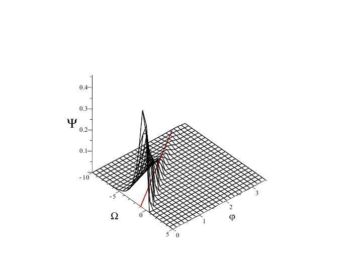
Figure 1: Exact wave function for the free case, i.e. for $U(\varphi,\varsigma)=0$. The wave function (40) is peaked around the classical trajectory $\Delta\Omega\pm\frac{3}{p}\Delta\varphi=\rm\nu_{0}=const$, which is the solid line shown on the $\{\Omega,\varphi\}$ plane. For this case $\nu_{0}=-1$ in equation (42a)

the classical trajectory implies that $\frac{\Delta\varsigma}{\ell}+\frac{\Delta\varphi}{p}=0$, then there is the simple relation between the fields $\varphi$ and $\varsigma$,

$$\rm\Delta\varsigma=-\frac{\ell}{p}\Delta\varphi.$$

So, the wavefunction can be written in terms of $\varphi$ and $\Omega$,

$$\rm\Psi(\Omega,\varphi,\varsigma)=e^{\frac{k}{2}\left(\Delta\Omega\pm\frac{3}{p}\Delta\varphi\right)+\frac{Q}{2}\Delta\Omega}\,\,Exp\left[{-{g_{0}h_{0}}e^{3\left(\Omega\pm\frac{3}{p}\Delta\varphi\right)}}\right],$$ (41)

Using the equantion (39), we find the classical trajectory on the $\{\Omega,\varphi\}$ plane as

$$\Delta\Omega\pm\frac{3}{p}\Delta\varphi = \rm\nu_{0}=const,$$ (42a)

$$\Delta\varphi = \rm Ln\left[\frac{3g_{0}h_{0}}{4}\Delta\tau\right]^{\pm\frac{p}{9}},$$ (42b)

$$\Delta\varsigma = \rm Ln\left[\frac{3g_{0}h_{0}}{4}\Delta\tau\right]^{\mp\frac{\ell}{9}},$$ (42c)

$$\Delta\Omega = \rm Ln\left[\frac{3g_{0}h_{0}}{4}\Delta\tau\right]^{\frac{1}{3}}+\nu_{0},$$ (42d)

where the first equation corresponds to constant phase of the second exponential in the W function (36). The last equation gives the scale factor which goes as a power law expansion, in a stiff matter epoch.

V.1.2 Exponential scalar potential

For an exponential scalar potential, see the third line in table (2), the exact solution of the WDW equation and the classical solutions are similar to the last case, only we redefine the constants,

$$\ell\to\sqrt{\ell^{2}-c_{0}H_{0}},\qquad p\to\sqrt{p^{2}+c_{1}G_{0}}.$$

We present two solutions, depending of the value of the constant $\rm 9-c_{0}H_{0}-c_{1}G_{0}$; when $\rm 6<c_{0}H_{0}+c_{1}G_{0}<9$, the scale factor which goes as a power law expansion, and $\rm c_{0}H_{0}+c_{1}G_{0}=9$, the scale factor have an exponential behavior. The corresponding classical solutions are

1. Case $\rm 6<c_{0}H_{0}+c_{1}G_{0}<9$

   $$\Delta\Omega\pm\frac{3}{\sqrt{p^{2}+c_{1}G_{0}}}\Delta\varphi = \rm\nu_{1}=const,$$ (43a)

   $$\Delta\varphi = \rm Ln\left[\frac{(9-c_{0}H_{0}-c_{1}G_{0})g_{0}h_{0}}{12}\Delta\tau\right]^{\pm\frac{\sqrt{p^{2}+c_{1}G_{0}}}{9-c_{0}H_{0}-c_{1}G_{0}}},$$ (43b)

   $$\Delta\varsigma = \rm Ln\left[\frac{(9-c_{0}H_{0}-c_{1}G_{0})g_{0}h_{0}}{12}\Delta\tau\right]^{\mp\frac{\ell^{2}-c_{0}H_{0}}{9-c_{0}H_{0}-c_{1}G_{0}}},$$ (43c)

   $$\Delta\Omega = \rm Ln\left[\frac{(9-c_{0}H_{0}-c_{1}G_{0})g_{0}h_{0}}{12}\Delta\tau\right]^{\frac{3}{9-c_{0}H_{0}-c_{1}G_{0}}},$$ (43d)

   if the scale factor must have an inflationary behavior as a power law expansion, the exponent $\rm\frac{3}{9-c_{0}H_{0}-c_{1}G_{0}}>1$, so, the constants $\rm 6<c_{0}H_{0}+c_{1}G_{0}<9$.

2. Case $\rm c_{0}H_{0}+c_{1}G_{0}=9$

   Employing the equations (38) and (39), we choose this value before to realize the integration, obtaining

   $$\Delta\Omega\pm\frac{3}{\sqrt{p^{2}+c_{1}G_{0}}}\Delta\varphi = \rm\nu_{1}=const,$$ (44a)

   $$\Delta\varphi = \rm\frac{g_{0}h_{0}\sqrt{p^{2}+c_{1}G_{0}}}{12}\Delta\tau,$$ (44b)

   $$\Delta\varsigma = \rm-\frac{g_{0}h_{0}\sqrt{\ell^{2}-c_{0}H_{0}}}{12}\Delta\tau,$$ (44c)

   $$\Delta\Omega = \rm\frac{g_{0}h_{0}}{4}\Delta\tau,\qquad\Rightarrow\qquad A(\tau)=e^{\Omega}=A_{0}e^{\frac{g_{0}h_{0}}{4}\Delta\tau}.$$ (44d)

where the scale factor have an exponential behavior, which corresponding to inflationary epoch with exponential scalar fields.

VI Final remarks.

Under canonical quantization we were able to determine a family of potentials that allows as to find exact solutions in classical and quantum cosmology in the inflation era. Some of the potentials of this family satisfied the conditions that can cross the cosmological constant barrier $\omega_{{}_{DE}}=-1$, equation (18). One potential for which it to was not possible to solve analytically Genly et al., (2012), by means of dynamical systems is possible to show that crosses this barrier.

The exact quantum solutions to the Wheeler-DeWitt equation were found using the Bohmian like scheme (Bohm,, 1952) of quantum mechanics, using the amplitude-real-phase approach Moncrief & Ryan, (1991), where the ansatz to the wave function is $\rm\Psi(\ell^{\mu})=W(\ell^{\mu})e^{-S(\ell^{\mu})}$ includes the superpotential function S, which plays an important role in solving the Hamilton-Jacobi equation.

We presented the corresponding Einstein Klein Gordon equation for the quintom model, which is applied to the FRW cosmological model with a barotropic perfect fluid and cosmological constant as the matter content; the classical solutions are given in a quadrature form for constant scalar potentials, in an inflationary stage ($p=-\rho$) these solutions are related to the Sáez-Ballester formalism, Sáez & Ballester, (1986); J. Socorro et al., (2010); M. Sabido et al., (2010); J. Socorro et al., (2011). For the inflationary stage with a potential that is a product of exponentials of the fields we found two exact solutions, one with a potential expansion law and the other with an exponential one.

We emphasize that the quantum potential from the Bohm like formalism will work as a constraint equation which restricts our family of potentials found, see table (2), J. Socorro et al., (2010). in this work such a problem has been solved in order to find the quantum potentials, which was a more important matter for being able to find the classical trajectories, which were showed through graphics how the classical trajectory is projected from its quantum counterpart. We include some steps used to solve the imaginary like equation (26b) when we found the superpotential function S (27) and particular ansatz for the function W, we found the equation (32), and using the separation variables method we find the set of equations that were necessary to solve.

The recent astronomical data suggest the existence of the dark energy with negative pressure Perlmutter, et al. (1999), with ratio $\rm\omega_{{}_{DE}}$ between the pressure $\rm P_{{}_{DE}}$ and the energy density $\rm\rho_{{}_{DE}}$ seems to be near or less than -1, $\rm-1.62<\omega_{{}_{DE}}<-0.74,$ Melchiorri, et al. (2002). Following the equation (18), in order to have agreement with these observational results, considering $\rm V(\varsigma,\varphi)>0$ and $\rm V(\varsigma,\varphi)>6\varphi^{\prime 2}-6\varsigma^{\prime 2}$, then the kinetic terms satisfies $\rm\varsigma^{\prime 2}<\varphi^{\prime 2}$, so, the barotropic parameter $\rm\omega_{{}_{DE}}<-1$. In this case, the intensity of the phantom field $\rm\varphi$ is always larger than the intensity of the quintessence field $\rm\varsigma$. In other case, we have that $\rm\omega_{{}_{DE}}>-1$. The particular value corresponding to cosmological constant is when the kinetic terms are null or equal in both fields.

However, the strange properties of the phantom field (violation of energy conditions and related negative energy density, the theories are not quantum mechanically viable, either because they violate conservation of probability, or they have unboundedly negative energy density and lead to the absence of a stable vacuum state, Cline et al., (2004)). To avoid this kind of problem, one should consider theories where the interactions between phantom field and normal matter are as weak as possible, but we must allow the ghosts to interact gravitationally, since it is their gravitational interactions which are needed for them to have any cosmological consequences. For instance, in Nojiri & Odintsov, (2003, 2003), the authors include some generalizations of phantom cosmology with quantum contribution. Quantum effects may lead also to negative energy density or to negative pressure what may indicate that phantom corresponds to the effective description of some fundamental quantum field theory (QFT). Those authors mention that QFT can suggests some mechanism to introduce the phantom field at the early universe, and most of energy conditions are satisfied due to quantum effects.

References

• Copeland et al., (2006) Copeland, E.J., Sami, M., and Tsujikawa S.: Int. J. Mod. Phys. D 15 1753, (2006) [arXiv:hep-th 0603057].
• Feng, (2006) Feng, B.: [ArXiv:astro-ph/0602156].
• Cai et al., (2010) Cai, Y.F., Saridakis, E.N., Setare, M.R., and Xia, J.Q.: Phys. Rep. 493, 1 (2010).
• Guo, (2005) Guo, Z.K., Piao, Y.S., Zhang, X., and Zhang, Y.Z.: Phys. Lett. B 608, 177 (2005).
• Feng, (2005) Feng, B., Wang, X., and Zhang, X.: Phys. Lett. B 607, 35 (2005).
• Sadjadi, (2006) Sadjadi, H.M., and Alimohammadi, M.: Phys. Rev. D 74 (4), 043506 (2006).
• Guo, (2006) Guo, Z.K., Piao, Y.S., Zhang, X., and Zhang, Y.Z.: Phys. Rev. D 74 (12), 127304 (2006).
• Feng, (2006) Feng, B., Li, M., Piao, Y.S., and Zhang, X.: Phys. Lett. B 634, 101 (2006).
• Zhao, (2006) Zhao, W., and Zhang, Y.: Phys. Rev. D 73 (12) 123509 (2006).
• (10) Cai, Y.F., Li, M., Lu, J.X., Piao, Y.S., Qiu, T. and Zhang, X.: Phys. Lett. B 651,1 (2007)
• (11) Cai, Y.F., Qiu, T., Zhang, X., Piao, Y.S. and Li, M.: J. of High Energy Phys. 10 71 (2007).
• Alimohammadi, (2007) Alimohammadi, M. and Sadjadi, H.M.: Phys. Lett. B 648, 113 (2007).
• Lazkoz, (2007) Lazkoz, R., León, G. and Quiros, I. Phys. Lett. B 649, 103 (2007).
• (14) Cai, Y.F., Qiu, T., Brandenberger, R., Piao, Y.S., and Zhang, X.: J of Cosmology and Astroparticle Phys. 3, 13 (2008).
• (15) Cai,Y.F., and Wang, J.: Classical and Quantum Gravity 25 (16), 165014 (2008).
• Zhang, (2008) Zhang, S., and Chen, B.: Phys. Lett. B 669, 4 (2008).
• Sadeghi, (2008) J. Sadeghi, M.R. Setare, A. Banijamali and F. Milani Phys. Lett. B 662, 92, (2008).
• Nozari, (2009) Nozari,K., Setare, M.R., Azizi, T. and Behrouz, N.: Physica Scripta, 80 (2), 025901 (2009).
• Setare, (2009) Setare, M.R., and Saridakis, E.N.: Phys. Rev. D 79 (4), 043005 (2009).
• Setare et al., (2009) Setare, M.R., and Saridakis, E.N.: Int. Jour. of Mod. Phys. D 18 (4), 549 (2009).
• Sadeghi, (2009) Sadeghi, J., Setare, M.R. and Banijamali, A.: Phys. Lett. B 678,164 (2009)
• Qiu, (2010) Qiu, T.: Mod. Phys. Lett.A 25, 909 (2010).
• (23) Saridakis, E.N.: Nuclear Phys. B 830, 374 (2010).
• Amani, (2011) Amani, A.R. Int. J. of Theor. Phys. 50, 3078 (2011).
• Farajollahi, (2012) Farajollahi, H., Shahabi, A., and Salehi, A.: Astronomy & Astrophysics, Supplement 338, 205 (2012).
• song et al., (2005) Song-Kuan Guo, Yun-Song Piao, Xinmin Zhang and Yuan-Zhong Zhang Phys. Lett. B 608, 177 (2005). [arXiv:astro-ph/0410654]
• Chimento, (2009) Chimento, L.P., Forte, M., Lazkoz, R., and Richarte, M.G.: Phys. Rev. D 79 (4) 043502(2009).
• Adak et al., (2011) Adak, D., Bandyopadhyay, A., and Majumdar, D.: (2011) [arXiv:1103.1533]
• Guzmán et al., (2007) Guzmán, W., Sabido, M., Socorro,J., and Ureña-López, L. Arturo.: Int. J. Mod. Phys. D 16 (4), 641-653 (2007).
• J. Socorro et al., (2010) Socorro, J., and D’oleire, M.: Phys. Rev. D 82(4), 044008 (2010).
• Bohm, (1952) Bohm, D.: Phys. Rev. 85 (2), 166 (1952).
• Moncrief & Ryan, (1991) Moncrief, V., and Ryan, M.P.: Phys. Rev. D 44, 2375 (1991).
• Kodama, (1988) Kodama, H.: Progress of Theor. Phys. 80, 1024 (1988).
• Kodama, (1990) Kodama, H.: Phys. Rev D 42, 2548 (1990).
• Melchiorri, et al. (2002) Melchiorri, A., Mersini, L., Odmann, C.J. and Trodden, M.: Astro-ph/0211522.
• Sáez & Ballester, (1986) Sáez, D., and Ballester, V.J.: Physics Letters A 113, 467 (1986).
• J. Socorro et al., (2010) Socorro, J., Sabido, M., Sánchez G., M.A. and Frías Palos, M.G.: Rev. Mex. Fís. 56(2), 166-171 (2010), [arxiv:1007.3306].
• M. Sabido et al., (2010) Sabido, M., Socorro, J. and Ureña-López, L. Arturo: Fizika B 19 (4), 177-186 (2010), [arXiv:0904.0422].
• J. Socorro et al., (2011) Socorro, J., Paulo A. Rodríguez, Espinoza-García, A., Pimentel, Luis O., and Romero, P.: Cosmological Bianchi Class A Models in Sáez-Ballester Theory: in Aspects of Today’s Cosmology InTech, Antonio Alfonso-Faus (Ed.) pages 185-204. Available from: http://www.intechopen.com/articles/show/title/
• Hartle & Hawking, (1983) J. Hartle, & S.W. Hawking Phys. Rev. D, 28, 2960 (1983).
• Arkadiusz & Jerzy, (1996) Blaut, A., and Kowalski G, J.: Class. Quantum Grav. 13,39 (1996).
• Barbosa & Pinto-Neto, (2004) Barbosa, G.D. and Pinto-Neto, N.: Phys. Rev. D 70 103512 (2004).
• Genly et al., (2012) León, G., Leyva, Y., and Socorro, J.: [gr-qc.1208-0061]
• Perlmutter, et al. (1999) Perlmutter, S. et al, Astrophys. J 517, 565 (1999).
• Cline et al., (2004) Cline, J.M., Jeon S. and Moore, G.D.: Phys. Rev. D 70, 043543 (2004).
• Nojiri & Odintsov, (2003) Nojiri, S. and Odintsov, S.D.: Phys. Lett. B 571, 1 (2003)).
• Nojiri & Odintsov, (2003) Nojiri, S. and Odintsov, S.D.: Phys. Lett. B 562, 147 (2003).