Magnetic proximity effect in the 3D topological insulator/ferromagnetic insulator heterostructure

Abstract

We theoretically study the magnetic proximity effect in the three dimensional (3D) topological insulator/ferromagnetic insulator (TI/FMI) structures in the context of possibility to manage the Dirac helical state in TI. Within continual approach based on the $\mathbf{kp}$ Hamiltonian we predict that, when 3D TI is brought into contact with 3D FMI, the ordinary bound state arising at the TI/FMI interface becomes spin polarized due to the orbital mixing at the boundary. Whereas the wave function of FMI decays into the TI bulk on the atomic scale, the induced exchange field, which is proportional to the FMI magnetization, builds up at the scale of the penetration depth of the ordinary interface state. Such the exchange field opens the gap at the Dirac point in the energy spectrum of the topological bound state existing on the TI side of the interface. We estimate the dependence of the gap size on the material parameters of the TI/FMI contact.

I INTRODUCTION

The engineering of layered hybrid heterostructures for spintronics applications, which are apt to simultaneously generate, manipulate and detect electron spin-polarized currents, sends a formidable challenge to modern material science and technology.Wolf The information obtained from combining traditional semiconductors with magnetic materials indicates the key influence of the interface between the constituents on magnetic properties of the heterostructure.Zutic ; Jansen The electronic rearrangement at the interface, often accompanied by appearance of spin-polarized bound states on both sides of the boundary, is the central feature inherent in the hybrid heterostructures. This feature underlies the magnetic proximity effect when spin ordering penetrates inside semiconductor over the interface.Men-10 Naturally one asks what are the peculiarities of the magnetic proximity effect provided that a trivial band semiconductor in the hybrid heterostructure is replaced by a time-reversal-invariant semiconductor with inverted band gap driven by strong intrinsic spin-orbit coupling (SOC), which is now known as a three dimensional topological insulator (3D TI).Hasan ; Qi A characteristic feature of the heterostructures containing the 3D TI layers is the topologically protected electron helical states with the linear Dirac-cone-like energy-momentum dispersion living at a boundary between topologically nonequivalent regions (such as between TI and a conventional, i.e. topologically trivial, insulator).Hasan ; Qi When TI is in contact with a magnetic material, the interface states can be influenced by a presence of magnetic ordering via time reversal symmetry breaking. Because of the Dirac spectrum and spin-momentum locking in such the systems, an interplay between the interface states and magnetism is naturally expected to display novel behavior that is absent in the case of the heterostructure composed of a conventional semiconductor and a magnetic material. In integrating of TIs with magnetic materials, fundamental issue is characterization of electron properties of the interface to understand the mechanisms of an exchange coupling.

The design of the heterostructures made of TI and magnetic layers has the potential to achieve a strong and uniform exchange coupling between the layers without significant spin dependent random scattering of helical carriers on magnetic atoms. The main challenge is to find suitable magnetic material, which can form a high-quality contact with TI and, at the same time, provides a strong exchange coupling at the interface. Unfortunately magnetic metals are out of the range of the search since they naturally short circuit the TI layer, restricting fundamentally the device design. The film of a ferromagnetic insulator or semiconductor (below we will use the abbreviation FMI) adjacent to TI is a most promising candidate to manipulate the helical states of 3D TI by means of a magnetic proximity effect.Garate Such a way may diminish the surface scattering via continuum states of the magnetic film, contrary to the metallic film case. There are several experimental investigations directly addressable to the hybrid TI/FMI structures. Zhou et al had studied semiconductor trilayer structures with ferromagnetic Sb_2-xCr_xTe₃ layers separated by the Sb₂Te₃ layer.Zhou Ferromagnetic out-of-plane exchange coupling between the Sb_2-xCr_xTe₃ layers was found for a sample with the Sb₂Te₃ spacer thickness of 2 nm. Recently Kandala et al. studied hybrid heterostructure composed of TI (Bi₂Se₃) and FMI (GdN) layers to probe the effects of broken time reversal symmetry on electrical transport in the surface states of 3D TI.Kandala Low temperature longitudinal magnetoconductance data presented in Ref. Kandala, are consistent with the opening of a magnetic gap in the surface state spectrum at the Bi₂Se₃/GdN interface. In Ref. Ji, it is demonstrated that the layered room temperature ferromagnet Fe₇Se₈ grows very well between layers of Bi₂Se₃ in bulk crystals. Both phases in the intergrown composite Bi₂Se₃:Fe₇Se₈ crystals display their intrinsic bulk properties: the ferromagnetism of Fe₇Se₈ is anisotropic, with magnetization easy axis in the plane of the crystal, and ARPES characterization shows that the topological states remain present on the Bi₂Se₃ surface. The heterostructures comprised of the layers of hexagonal TI Bi₂Se₃ and cubic FMI EuS with the sharp interface were fabricated by molecular beam epitaxy in Ref. Wei, . The magnetic and magnetotransport measurements on the Bi₂Se₃/EuS bilayers indicated eloquently that EuS induces ferromagnetic order with a significant magnetic moment in the interfacial region of the Bi₂Se₃ layer due to a transmission of the exchange field across the interface.Wei

Of magnetic insulators that show relatively good lattice matching with binary TIs Bi₂Te₃, Bi₂Se₃ and Sb₂Te₃, one can note the wide-gap antiferromagnetic insulator (AFMI) MnSe.Luo The authors of Ref. Luo, performed first-principles calculation for the Bi₂Se₃/MnSe superlattice electron structure; in particular, they predicted that exchange coupling with MnSe induces a gap of 54 meV in the surface states spectrum of Bi₂Se₃.

There are theoretical studies of the properties of TI in contact with a conventional FMI, which are routinely based on the simple phenomenological Hamiltonian of the 2D Dirac-like states of helical fermions in an homogeneous exchange field:Fu $H_{s}=-iv(\mathbf{e}_{z}[\bm{\sigma}\times\bm{\bigtriangledown}])+\mathbb{U}_{ex}$, where $\mathbf{e}_{z}$ is the unit vector normal to the interface, $v$ is the Fermi velocity. It is generally thought that a controllable exchange field on the TI side of the TI/FMI hybrid structure can be directly generated by means of a FMI layer attached to a TI layer.Garate ; Tserkovnyak ; Yokoyama In such the case one presumes $\mathbb{U}_{ex}=J(\bm{\sigma}\mathbf{M})$, i.e., the exchange field is proportional to the FMI magnetization $\mathbf{M}$ on the FMI side of the structure, $J$ is effective exchange coupling and $\bm{\sigma}$ is the vector composed of the Pauli matrices. Within this description, it was predicted that many curious effects can be realized in the TI/FMI structures. However, strictly speaking, the 2D Hamiltonian $H_{s}$ can formally be derived from a relevant 3D Hamiltonian only under the stipulation that TI has a free surface on which $\mathbb{U}_{ex}=0$. Usually, to take into account a perturbation from the interface with magnetic material, the exchange term is simply included in the Hamiltonian $H_{s}$, without a serious analysis of its microscopic origin. The same one can refer to an attempt to go beyond the scope of the 2D model.Habe

In the present paper, within the framework of the continual approach, we study the physics of magnetic proximity effect at the TI/FMI heterocontact. This model generalizes an approach recently proposed to describe the electron states formed by the interface between TI and normal insulator (NI).Men-13 As was shown in Ref. Men-13, the boundary between TI and a trivial insulator hosts a pair of the bound electron states inside the bulk energy gap of TI on the topological side of the interface (referred as the topological and ordinary states), which differ from each other in physical meaning, spatial distribution and energy spectrum. Namely, the bound topological state stems from a breaking of the $Z_{2}$ topological invariant at the boundary with a trivial insulator. This state being located relatively remote from the interface and almost insensitive to the interface influence shows the Dirac spectrum. By contrast, the bound ordinary state results from the crystal symmetry breaking at the interface. This state is spatially located near the interface, therefore, its features strongly depend on the effective interface potential. Here we generalize the approach of Ref. Men-13, to the case when TI is attached to FMI. Our analysis sheds light on the origin of the proximity effect in the TI/FMI structures and the possibility of magnetic control over the Dirac helical state in TI.

The paper is organized as follows. In Sec. II, we discuss the model for a contact between TI and FMI and introduce the main ingredients and assumptions of the problem within the continual approach, which takes into account the hybridization between the orbitals of the constituents at the interface. In Sec. III, we argue the occurrence of the spin-polarized ordinary interface state on the topological side of the contact, derive the spin polarization of carriers in the ordinary state that is induced by the adjacent FMI and determine the dependence of the polarization on the distance from the interface. In Sec. IV the behavior of the topological interface state under the influence of the exchange field associated with the ordinary state is described. We show how the proximity of the FMI modifies the energy spectrum of the topological state and obtain the expression for the energy gap. In Sec. V, we analyze the obtained results and compare them with the recent ab-initio calculations for the Bi₂Se₃/MnSe superlattice.Eremeev

II MODEL HAMILTONIAN

We consider a conceptual analytic model for the magnetic proximity effect in the TI/FMI structure. The low energy and long wavelength bulk electron states of the prototypical TI, narrow-gap semiconductor of Bi₂Se₃-type, are described near the $\Gamma$ point of the Brillouin zone by the four bands $\mathbf{kp}$ Hamiltonian with strong SOC proposed in Ref. Liu, . Without a loss of generality, we make use the simplified version of this Hamiltonian in the form:

$$H_{t}^{0}(\mathbf{k})=\Xi(\mathbf{k})\tau_{z}\otimes\sigma_{0}+\mathrm{A}(k_{x}\tau_{x}+k_{y}\tau_{y})\otimes\sigma_{x}+\mathrm{A}k_{z}\tau_{x}\otimes\sigma_{z},$$ (1)

where $\Xi(\mathbf{k})=\Xi-\mathrm{B}k^{2}$, $\mathbf{k}$ is the wave vector, $k=|\mathbf{k}|$, $\sigma_{\alpha}$ and $\tau_{\alpha}$ ($\alpha=0,x,y,z$) denote the Pauli matrices in the spin and orbital space, respectively. The condition $\Xi,\mathrm{B}>0$ reflects an inverted order of the energy terms around the $\Gamma$ point $\mathbf{k}=0$ as compared with large $k$, which correctly characterizes the topologically non-trivial nature of the system due to strong SOC.

For the sake of simplicity we introduce the FMI as a wide-gap semiconductor in which the exchange potential of local magnetic moments induces uniform spin splitting of both the conduction and valence bands in the bulk. Thus, the low energy and long wavelength bulk electron states of FMI are formally modeled by the four bands $\mathbf{kp}$ Hamiltonian without SOC:

$$H_{f}^{0}(\mathbf{k})=\mathrm{E}_{0}(\mathbf{k})\mathbb{I}+\Lambda(\mathbf{k})\tau_{z}\otimes\sigma_{0}+\mathrm{M}\tau_{0}\otimes\sigma_{z},$$ (2)

where $\mathbb{I}$ is unit $4\times 4$ matrix. For the sake of convenience we use a simple effective mass approximation so that $\Lambda(\mathbf{k})=\Lambda+\mathrm{N}k^{2}$, $\Lambda,\mathrm{N}>0$. The band structure (2) is generally asymmetric with respect to the middle of the TI band gap, since $\mathrm{E}_{0}(\mathbf{k})\neq 0$; in the following we omit for simplicity the $\mathbf{k}$ dependence of $\mathrm{E}_{0}(\mathbf{k})$ and put $\mathrm{E}_{0}(\mathbf{k})=\mathrm{E}_{0}$. The intrinsic magnetization of FMI is assumed perpendicular to the TI/FMI interface plane. We regard FMI as a wide-gap semiconductor in the sense that $|\mathrm{E}_{c,v}^{\sigma}|>\Xi$, where $\mathrm{E}_{c}^{\sigma}=\mathrm{E}_{0}+\Lambda+\sigma\mathrm{M}$ and $\mathrm{E}_{v}^{\sigma}=\mathrm{E}_{0}-\Lambda+\sigma\mathrm{M}$ are the edges of the conduction and valence bands, respectively, $\Lambda,\mathrm{M}>0$, $\sigma=\pm 1$ is spin projection on the quantization axis $z$.

We assume that the TI occupies the right half-space, $z>0$, while the FMI occupies the left one, $z<0$. Both the TI and FMI are treated as semi-infinite materials joined at a perfectly flat interface located at $z=0$. In a real space coordinate representation, the electron energy of the TI/FMI contact reads:

$$\Omega = \int_{z>0}d\mathbf{r}\Theta^{{\dagger}}(\mathbf{r})H_{t}(-i\nabla)\Theta(\mathbf{r})$$

$$+ \int_{z<0}d\mathbf{r}\Phi^{{\dagger}}(\mathbf{r})H_{m}(-i\nabla)\Phi(\mathbf{r})+\Omega_{I},$$

$$H_{t}(-i\nabla)=H_{t}^{0}(-i\nabla)+\varphi(\mathbf{r})\mathbb{I}+\tau_{0}\otimes(\bm{\sigma}\cdot\bm{\Delta}(\mathbf{r})),$$ (4)

$$H_{f}(-i\nabla)=H_{f}^{0}(-i\nabla)+\varphi_{m}(\mathbf{r})\mathbb{I}+\tau_{0}\otimes(\bm{\sigma}\cdot\bm{\Delta}_{m}(\mathbf{r})),$$ (5)

$$\Omega_{I}=\int d\mathbf{r}[\Theta^{{\dagger}}(\mathbf{r})V(\mathbf{r})\Phi(\mathbf{r})+\Phi^{{\dagger}}(\mathbf{r})V^{{\dagger}}(\mathbf{r})\Theta(\mathbf{r})],$$ (6)

Here the operators $H_{t}^{0}(-i\nabla)$ and $H_{f}^{0}(-i\nabla)$ determined in Eqs. (1)-(2) (momentum $\mathbf{k}$ is replaced by operator $-i\nabla$) act in the space of the spinor envelope functions $\Theta(\mathbf{r})=(\theta_{1}(\mathbf{r}),\theta_{2}(\mathbf{r}),\theta_{3}(\mathbf{r}),\theta_{4}(\mathbf{r}))^{\mathrm{T}}$ and $\Phi(\mathbf{r})=(\phi^{(1)}(\mathbf{r}),\phi^{(2)}(\mathbf{r}),\phi^{(3)}(\mathbf{r}),\phi^{(4)}(\mathbf{r}))^{\mathrm{T}}$, respectively. The subscript $j$ indicates the TI state spinor components, $\theta_{j}(\mathbf{r})$, while the superscript $(n)$ indicates the FMI state spinor components, $\phi^{(n)}(\mathbf{r})$.

Since TI is a narrow-gap semiconductor, it is evident that a significant electric field can be induced on the TI side of the TI/FMI contact due to the redistribution of the charge density of carriers $n(\mathbf{r})$ in the sub-interface layers of TI. This field contains, in principle, the components of different spatial scales. In our approach, the short-range (of the order of inter-atomic distance) components of the Coulomb potential are assumed to be included in the spin-independent terms of an effective local interface potential (see below). The long-range profile of the Coulomb potential $\varphi(\mathbf{r})$ in Eq. (4) near the interface can be formally described by the equation

$$\varphi(\mathbf{r})=\int d\mathbf{r}^{\prime}\mathcal{V}(\mathbf{r}-\mathbf{r}^{\prime})n(\mathbf{r}^{\prime}),$$ (7)

where $\mathcal{V}(\mathbf{r})$ is the spin-independent part of electron-electron interaction in TI. Besides, a noticeable redistribution of the carrier spin density $s(\mathbf{r})$ can appear in TI due to exchange coupling between the states of TI and FMI at the interface. This redistribution induces an exchange field in the sub-interface layers of TI. In our approach, the short-range components of this field are included into the spin-dependent terms of an effective local interface potential (see below), while the relative long-range components of the spin density cause the spin-dependent field $\bm{\Delta}(\mathbf{r})$ in Eq. (4):

$$\Delta^{\alpha}(\mathbf{r})=\int d\mathbf{r}^{\prime}\mathcal{K}^{\alpha\beta}(\mathbf{r}-\mathbf{r}^{\prime})s^{\beta}(\mathbf{r}^{\prime}).$$ (8)

The diagonal elements of the matrix $\mathcal{K}^{\alpha\beta}(\mathbf{r})$ with $\alpha=\beta$ are due to the exchange term of the electron-electron interaction in TI, while the off-diagonal elements with $\alpha\neq\beta$ appear due to the spin-flip electron-electron scattering and vanish without SOC.

In general case, not only the bound interface states under the study, but all engaged electron states of TI give rise to the charge and spin densities, $n(\mathbf{r})$ and $s(\mathbf{r})$. The fields $\varphi(\mathbf{r})$ and $\bm{\Delta}(\mathbf{r})$ in Eq. (4) are associated with the band bending and spin splitting on the TI side of the contact, respectively. It is clear that similar expressions can be formally written for the potentials $\varphi_{f}(\mathbf{r})$ and $\bm{\Delta}_{f}(\mathbf{r})$ on the MI side of the contact. However, since FMI is a wide-gap semiconductor, it is reasonable to assume in Eq. (5) that $|\varphi_{f}(\mathbf{r})|<<2\Lambda$ and $|\bm{\Delta}_{f}(\mathbf{r})|<<2\mathrm{M}$, thus neglecting the effect of charge and spin redistributions for the FMI subsystem.

To formally make the potentials $\varphi(\mathbf{r})$ and $\Delta^{\alpha}(\mathbf{r})$ [as well as the interactions $\mathcal{V}(\mathbf{r})$ and $\mathcal{K}^{\alpha\beta}(\mathbf{r})$] consistent with the densities $n(\mathbf{r})$ and $s(\mathbf{r})$ it is necessary to solve the system of the Dyson equations for the self-energy parts of the Green‘s functions on the TI side of the contact. One can hardly accomplish this task analytically, so we make some approximations. First, the matrices $\mathcal{V}(\mathbf{r})$ and $\mathcal{K}^{\alpha\beta}(\mathbf{r})$ are supposed to be independent of the orbital indices. Second, we use the ”local” approximation for an electron-electron interaction: $\mathcal{V}(\mathbf{r})\rightarrow\mathcal{V}\delta(\mathbf{r})$ and $\mathcal{K}^{\alpha\beta}(\mathbf{r})\rightarrow\mathcal{K}^{\alpha\beta}\delta(\mathbf{r})$ [$\delta(\mathbf{r})$ is the delta-function], which is specific to a metal situation. For the Coulomb interaction such the assumption is not evident, since the effective scale of $\mathcal{V}(\mathbf{r})$ defined by the Debye screening length, $D$, may significantly exceed a characteristic metal screening length due to a relatively low carrier concentration in TI. Nevertheless, we formally suggest that, near the interface, the concentration $n(\mathbf{r})$ is large enough to efficiently screen the interaction between carriers. As for the exchange and spin-orbit components, the scale of $\mathcal{K}^{\alpha\beta}(\mathbf{r})$ is at least one order of magnitude lower as compared to $D$, hence in this case the ”local” approximation is correct. Third, we average the redistributions $n(\mathbf{r})$ and $s(\mathbf{r})$ over the $(x,y)$ plane remaining one-dimensional profiles $n(z)$ and $s(z)$. As a result of the aforesaid approximations we arrive at the following relations $\varphi(z)=\mathcal{V}n(z)$ and $\bm{\Delta}^{\alpha}(z)=\mathcal{K}^{\alpha\beta}s^{\beta}(z)$. This means that, in Eq. (4), we consider electrons under the one-dimensional potential fields, $\varphi(z)$ and $\bm{\Delta}^{\alpha}(z)$, smoothly varying (on an atomic scale) in the $z$ direction and homogeneous along the $(x,y)$ plane.

The $\mathbf{kp}$ method cannot provide information on the wave-function behavior in the vicinity of the atomically sharp interface, where large momenta are highly important. To overcome this drawback we bring in the effective potential of hybridization $V(\mathbf{r})$, which intermixes the TI and FMI electron states at the interface. The hybridization potential $V(\mathbf{r})$ spreads over a small region $d$ (of the order a lattice parameter) around the geometrical boundary $z=0$, where the $\mathbf{kp}$ scheme is not valid. An introduction of the phenomenological term of the interface energy $\Omega_{I}$ enables us to correctly reconcile the short-range (at $|z|<d<<D$) and long-range (at $|z|>d$) variations of the charge and spin densities near the interface in terms of the boundary conditions for the envelope functions $\Theta(\mathbf{r})$ and $\Phi(\mathbf{r})$. The influence of the short-range variations of $n(\mathbf{r})$ and $s(\mathbf{r})$ is implied to be included into the effective potential of the hybridization. As long as the spatial variations of the interface states are sufficiently slow on the scale of the length $d$, one can adopt for practical calculations a local approximation for the hybridization potential, $V(\mathbf{r})=dV(x,y)\delta(z)$.

III SPIN POLARIZED ORDINARY BOUND STATE

Since the system under consideration displays translational symmetry in the interface plane, it is reasonable to use the mixed $(\bm{\kappa},z)$ representation, where $\bm{\kappa}$ is 2D wave vector in the $(x,y)$ plane. We are interested in obtaining the eigen states of the problem, Eqs. (II)-(6), with decaying asymptotics far from the interface, $\Phi(\bm{\kappa},z\rightarrow-\infty)$ and $\Theta(\bm{\kappa},z\rightarrow\infty)$. Recently, within the variational approach, it was shownMen-13 that the energy functional Eq. (II) possesses two different extremals on the class of piecewise smooth in both half-spaces and square integrable functions. In other words, for each $\kappa$-mode, one can write the spinor envelope functions $\{\Phi(\bm{\kappa},z),\Theta(\bm{\kappa},z)\}$ satisfying the same Euler equation, $[H_{m}(\bm{\kappa},-i\partial_{z})-E]\Phi(\bm{\kappa},z)=0$ at $z<0$ and $[H_{t}(\bm{\kappa},-i\partial_{z})-E]\Theta(\bm{\kappa},z)=0$ at $z>0$ (where $\partial_{z}=\partial/\partial z$), but distinct boundary conditions at the interface $z=0$. On the one hand, one can strictly fix the magnitude of the envelope functions at the interface, $\{\Phi(\bm{\kappa},0-)=0,\Theta(\bm{\kappa},0+)=0\}$ to obtain the so-called interface topological state $\{\Phi_{t}(\bm{\kappa},z),\Theta_{t}(\bm{\kappa},z)\}$.Men-13 This case will be considered later on. Now we focus on the so-called interface ordinary state with the envelope function $\{\Phi_{o}(\bm{\kappa},z),\Theta_{o}(\bm{\kappa},z)\}$ corresponding to the natural boundary conditions:Men-13

$$i\frac{\delta H_{t}(\bm{\kappa},-i\partial_{z})}{\delta(-i\partial_{z})}\Theta(\bm{\kappa},z)|_{z=0+}-2dV(\bm{\kappa})\Phi(\bm{\kappa},z)|_{z=0-}=0,$$ (9)

$$i\frac{\delta H_{m}(\bm{\kappa},-i\partial_{z})}{\delta(-i\partial_{z})}\Phi(\bm{\kappa},z)|_{z=0-}-2dV^{{\dagger}}(\bm{\kappa})\Theta(\bm{\kappa},z)|_{z=0+}=0.$$ (10)

In the left half-space, the components of the envelope function $\Phi_{o}(\bm{\kappa},z)$ are given by:

$$\phi^{(n)}(\bm{\kappa},z)=\phi^{(n)}(\bm{\kappa},0)\exp[p^{(n)}(\kappa)z],$$ (11)

$$\phi^{(n)}(\bm{\kappa},0)=\frac{(-1)^{n+1}d}{\mathrm{N}p^{(n)}(\kappa)}\sum_{j=1}^{4}V_{j}^{(n)\ast}(\kappa)\theta_{j}(\bm{\kappa},0),$$ (12)

$$p^{(1)}(\kappa)=\sqrt{\kappa^{2}+[\Lambda+\mathrm{E}_{0}-E+\mathrm{M}]/\mathrm{N}},$$ (13)

$$p^{(2)}(\kappa)=\sqrt{\kappa^{2}+[\Lambda-\mathrm{E}_{0}+E+\mathrm{M}]/\mathrm{N}},$$ (14)

$$p^{(3)}(\kappa)=\sqrt{\kappa^{2}+[\Lambda+\mathrm{E}_{0}-E-\mathrm{M}]/\mathrm{N}},$$ (15)

$$p^{(4)}(\kappa)=\sqrt{\kappa^{2}+[\Lambda-\mathrm{E}_{0}+E-\mathrm{M}]/\mathrm{N}},$$ (16)

where $V_{j}^{(n)}(\kappa)$ are the matrix elements of the hybridization potential $V(\mathbf{r})$, the subscript $j$ and superscript $(n)$ are related to the TI and FMI states, respectively.

Inserting $\Phi(\bm{\kappa},0)$ Eq. (12) into Eq. (9) one arrives at the relation for the interface magnitude of the ordinary envelope function on the TI side:

$$i\frac{\delta H_{t}(\bm{\kappa},-i\partial_{z})}{\delta(-i\partial_{z})}\Theta(\bm{\kappa},0)-2dU(\bm{\kappa},E)\Theta(\bm{\kappa},0)=0,$$ (17)

which contains the effective local pseudo-potential $U(\bm{\kappa},E)$ seen by electrons on the TI side. The potential matrix elements have the form

$$U_{jj^{\prime}}(\bm{\kappa},E)=\sum_{n=1}^{4}(-1)^{n+1}U_{jj^{\prime}}^{(n)}(\bm{\kappa},E),$$ (18)

$$U_{jj^{\prime}}^{(n)}(\bm{\kappa},E)=\frac{dV_{j}^{(n)}V_{j^{\prime}}^{(n)\ast}}{\mathrm{N}p^{(n)}(\kappa,E)}.$$ (19)

The matrix elements $U_{jj^{\prime}}^{(n)}(\bm{\kappa},E)$ characterize internal properties of the interface. In the case when $V^{(n)}_{1,3}\neq 0$, $V^{(n)}_{2,4}=0$, the effective pseudo-potential $U(\bm{\kappa},E)$ has four non-zero components: $U_{11}(\bm{\kappa},E)=P(\bm{\kappa},E)+Q(\bm{\kappa},E)$, $U_{33}(\bm{\kappa},E)=P(\bm{\kappa},E)-Q(\bm{\kappa},E)$, $U_{13}(\bm{\kappa},E)=U_{31}^{\ast}(\bm{\kappa},E)$, where $P(\bm{\kappa},E)$, $Q(\bm{\kappa},E)$ and $U_{13}(\bm{\kappa},E)$ are the potential, exchange and spin orbit contribution(s), respectively. These expressions are derived under the condition $|U_{13}(\bm{\kappa},E)|<<|Q(\bm{\kappa},E)|<<|P(\bm{\kappa},E)|$; note, that $Q(\bm{\kappa},E)$ is proportional to the intrinsic exchange potential $\mathrm{M}$ of the FMI Hamiltonian, Eq. (2). In the following, for the sake of simplicity, we omit the dependence of $P(\bm{\kappa},E)$, $Q(\bm{\kappa},E)$ and $U_{13}(\bm{\kappa},E)$ on both $\bm{\kappa}$ and $E$. Then, if the hybridization with the FMI conduction band is predominant, one obtains the estimation

$$P\simeq\frac{d|V|^{2}}{\mathrm{N}\sqrt{\Lambda+\mathrm{E}_{0}}},~{}Q\simeq\frac{-d|V|^{2}\mathrm{M}}{2\mathrm{N}(\sqrt{\Lambda+\mathrm{E}_{0}})^{3}},~{}U_{13}\simeq\frac{dV_{1}^{(1)}V_{3}^{(1)\ast}}{\mathrm{N}\sqrt{\Lambda+\mathrm{E}_{0}}},$$ (20)

where $\Lambda+\mathrm{E}_{0}>>\mathrm{M}$, $|V^{(1)}_{1}|=|V^{(3)}_{3}|=|V|$. The influence of the off-diagonal component of the hybridization, $U_{13}$, on the interface electron states has been discussed in Ref. Men-13, . This influence is insignificant as the interface spin-flip processes generating the component $U_{13}$ are relatively weak, $|V_{3}^{(1)}|\approx|V_{1}^{(3)}|<<|V|$. We are interested in the investigation of the interface state spin polarization along the $z$ axis. Therefore in the following, without the loss of generality, we assume $U_{13}=0$. As a consequence, the matrix $\mathcal{K}^{\alpha\beta}$ acquires the diagonal form and the $z$-polarized exchange field is $\Delta^{z}(z)=\mathcal{K}^{zz}s^{z}(z)$. Below the upper indices can be omitted, i.e., $\Delta(z)=\mathcal{K}s(z)$.

In general case, under the nontrivial boundary conditions and the self-consistent potentials $\varphi(z)$ and $\Delta(z)$, we meet a problem to seek for the solution of the non-linear equation $[H_{t}(\bm{\kappa},-i\partial_{z})-E]\Theta(\bm{\kappa},z)=0$ (at $z>0$). It is evident, no exact analytical solution for such the task is available. Therefore, to capture the principal features of the solution, we restrict ourselves to the lowest order of perturbation theory in the interface potential and disregard the feedback influence of these potentials on the envelope function and spectrum the ordinary bound state. As it will be shown below, the weak interface potential approximation, even being relatively simplified, gives a good opportunity to clearly understand what role the ordinary bound state plays in the establishing of an exchange field on the TI side of the contact.

Following the procedure of Ref. Men-13, one can obtain the expressions for the spectrum $E_{o}(\kappa)$ of the interface ordinary state and the envelope function $\Theta_{o}(\bm{\kappa},z)$ at $z>0$. If the interface potential is weak, $|P,Q|/\Xi<<1$, the ordinary state spectrum for small momenta is given by the transparent formula:

$$E_{o}^{(\pm)}(\kappa)=-\widetilde{P}\pm\sqrt{\widetilde{Q}^{2}+\mathrm{A}^{2}\kappa^{2}},$$ (21)

$$\widetilde{P}=\frac{2dP\sqrt{\Xi}}{\sqrt{\mathrm{B}}}\frac{\sqrt{\lambda}}{1+\lambda},~{}\widetilde{Q}=\frac{2dQ\sqrt{\Xi}}{\sqrt{\mathrm{B}}}\frac{\sqrt{\lambda}}{1+\lambda},$$ (22)

where $\lambda=\mathrm{A}^{2}/4\mathrm{B}\Xi$ is the parameter of the TI bulk band spectrum, which is implied to be $\lambda\geqslant 1$. The spin-independent part of the interface potential gives the energy shift $-\widetilde{P}$ to the dispersion relation, while the $z$ component of the exchange part of the interface potential causes the energy gap of the size $2\widetilde{Q}$ at the node point; the label $\pm$ in Eq. (21) distinguishes the states above and below the gap.

Keeping the first order in the terms of the interface potential, after some algebra, the envelope function of the ordinary state with spin projection $\sigma=\pm$, $\Theta_{o}^{\sigma}(\bm{\kappa},z)$, is reduced to rather simple form

$$\Theta_{o}^{\sigma}(\bm{\kappa},z) = C_{o}^{\sigma}(\kappa)\{\Theta_{1}^{\sigma}(\phi)\exp[-q_{1}(\kappa)z]$$

$$+ \Theta_{2}^{\sigma}(\phi)\exp[-q_{2}(\kappa)z]\},$$

$$\Theta_{1}^{\sigma}(\phi) = (i(1+\alpha_{1}^{\sigma}),sign(\mathrm{A})(1+\alpha_{2}^{\sigma}),$$

$$e^{i\phi}(1+\alpha_{1}^{-\sigma}),sign(\mathrm{A})ie^{i\phi}(1+\alpha_{2}^{-\sigma}))^{\mathrm{T}},$$

$$\Theta_{2}^{\sigma}(\phi) = (i(1+\beta_{1}^{\sigma}),sign(\mathrm{A})(1+\beta_{2}^{\sigma}),$$

$$e^{i\phi}(1+\beta_{1}^{-\sigma}),sign(\mathrm{A})ie^{i\phi}(1+\beta_{2}^{-\sigma}))^{\mathrm{T}},$$

where $C_{o}^{\sigma}(\kappa)$ is normalization factor. The corrections $\alpha_{j}^{\sigma}$ and $\beta_{j}^{\sigma}$ satisfy the relations:

$$-\widetilde{P}+\sigma\widetilde{Q} = |\mathrm{A}|q_{1}(\alpha_{1}^{\sigma}-\alpha_{2}^{\sigma})=|\mathrm{A}|q_{2}(\beta_{1}^{\sigma}-\beta_{2}^{\sigma})$$

$$= |\mathrm{A}|[q_{1}-q_{2}](\beta_{2}^{\sigma}-\alpha_{2}^{\sigma})/4$$

$$= \mathrm{B}\Xi[q_{1}-q_{2}](\beta_{1}^{\sigma}-\alpha_{1}^{\sigma})/|\mathrm{A}|.$$

The characteristic momenta are given by

$$q_{1}(\kappa)=\frac{|\mathrm{A}|+\sqrt{\mathrm{A}^{2}-4\mathrm{B}\Xi(\kappa)}}{2\mathrm{B}},$$ (27)

$$q_{2}(\kappa)=\frac{|\mathrm{A}|-\sqrt{\mathrm{A}^{2}-4\mathrm{B}\Xi(\kappa)}}{2\mathrm{B}},$$ (28)

and $q_{1,2}=q_{1,2}(0)$, $\Xi(\kappa)=\Xi-\mathrm{B}\kappa^{2}$. We neglect a weak dependence of the pre-exponential factors $\Theta_{1,2}^{\sigma}(\phi)$ (III)-(III) on $\kappa$. The corrections $\alpha_{j}^{\sigma}$ and $\beta_{j}^{\sigma}$ reflect the fact that the interface potential lifts both the electron-hole degeneration and the spin degeneration of the TI bulk Hamiltonian (1). From Eq. (III) it is clear that, when $Q\neq 0$, one has $\alpha_{j}^{\sigma}\neq\alpha_{j}^{-\sigma}$ and $\beta_{j}^{\sigma}\neq\beta_{j}^{-\sigma}$. Without the interface potential the corrections are absent, $\alpha_{j}^{\sigma}=0$ and $\beta_{j}^{\sigma}=0$. The probability density of the ordinary state (III), $|\Theta_{o}^{\sigma}(\bm{\kappa},z)|^{2}$, shows the maximum value at $z=0$ and decays exponentially into TI with the characteristic length $z_{o}\simeq q_{2}^{-1}$.

The charge density $n_{o}(z)$ and spin density $s_{o}(z)$ associated with the formation of the bound ordinary state on the TI side of the TI/FMI interface may be determined as $n_{o}(z)=\sum_{\bm{\kappa}}\Theta_{o}^{{\dagger}}(\bm{\kappa},z)(\frac{\mathbb{I}}{2})\Theta_{o}(\bm{\kappa},z)$ and $s_{o}(z)=\sum_{\bm{\kappa}}\Theta_{o}^{{\dagger}}(\bm{\kappa},z)\frac{\tau_{0}\sigma_{z}}{2}\Theta_{o}(\bm{\kappa},z)$, respectively, where the sum runs over occupied states. When the dispersion law is expressed by Eqs. (21)-(22), one can write these densities through the squared components of the envelope function (III) as

$$n_{o}(z) = \frac{a^{2}}{4\pi\mathrm{A}^{2}}\int_{-W}^{\mu}dE(E+\widetilde{P})$$

$$\times \biggl{[}h(E+\widetilde{P}-|\widetilde{Q}|)+h(-E-\widetilde{P}-|\widetilde{Q}|)\biggr{]}$$

$$\times \sum_{j=1}^{4}|\theta_{oj}^{+}(\bm{\kappa},z)|^{2},$$

$$s_{o}(z) = \frac{a^{2}}{4\pi\mathrm{A}^{2}}\int_{-W}^{\mu}dE(E+\widetilde{P})$$

$$\times \biggl{[}h(E+\widetilde{P}-|\widetilde{Q}|)+h(-E-\widetilde{P}-|\widetilde{Q}|)\biggr{]}$$

$$\times \biggl{[}|\theta_{o1}^{+}(\bm{\kappa},z)|^{2}-|\theta_{o2}^{+}(\bm{\kappa},z)|^{2}$$

$$+ |\theta_{o2}^{-}(\bm{\kappa},z)|^{2}-|\theta_{o1}^{-}(\bm{\kappa},z)|^{2}\biggr{]},$$

where $\mu$ is the chemical potential, $W$ is a cut-off energy, $W\simeq|\mathrm{A}|a^{-1}\simeq\Xi$, $a$ is in-plane lattice constant. In Eqs. (III) and (III), we have used the above relations (III).

The FMI magnetization opens the gap $2|\widetilde{Q}|$ in the ordinary state spectrum at the node point $E_{o}(0)$ being somewhat remote from the chemical potential $\mu$. Here we study the relevant regime of $\mu+\widetilde{P}>|\widetilde{Q}|$. In the leading non-vanishing order in the interface energies, which are far below the bulk energy gap, $\widetilde{P}<<\Xi$ and $|\widetilde{Q}|<<\Xi$, it is now straightforward to use Eqs. (III) and (III) to find that

$$n_{o}(z)\simeq\frac{2a^{2}|C_{o}|^{2}}{\pi\mathrm{A}^{2}}(W^{2}+\mu^{2})g_{o}(z),$$ (31)

$$g_{o}(z)=\frac{1}{4}\biggl{\{}\exp[-q_{1}z]+\exp[-q_{2}z]\biggr{\}}^{2},$$ (32)

$$s_{o}(z)\simeq\frac{2a^{2}|C_{o}|^{2}}{\pi\mathrm{A}^{2}}\frac{\widetilde{Q}}{\Xi}(W^{2}+\mu^{2})f(z),$$ (33)

$$f(z) = \frac{\Xi}{2|\mathrm{A}|}\biggl{\{}\exp[-q_{1}z]+\exp[-q_{2}z]\biggr{\}}$$

$$\times \biggl{\{}\frac{\exp[-q_{1}z]}{q_{1}}+\frac{\exp[-q_{2}z]}{q_{2}}\biggr{\}},$$

where $|C_{o}|^{2}=|C_{o}(0)|^{2}=|\mathrm{A}|/8\mathrm{B}(1+\lambda)$, $g_{o}(0)=f(0)=1$. Since the dependence of the function $\theta_{oj}^{\pm}(\bm{\kappa},z)$ on $\bm{\kappa}$ is weak enough, it has been justified to set $\bm{\kappa}=0$ in the integrand in Eqs. (III) and (III).

Thus, when TI is brought into contact with FMI, the hybridization between the orbitals of TI and FMI at the interface induces the spin polarized ordinary bound state on the topological side of the contact. The direction of spin polarization of this state is opposite to the FMI magnetization, the magnitude $s_{o}(0)$ is proportional to $\widetilde{Q}\sim\mathrm{M}$ and depends on the occupation of the state. Thank to the ordinary spin polarized state, the induced exchange field $\Delta_{o}(z)=\mathcal{K}s_{o}(z)$ penetrates inside TI on the length scale far above the lattice spacing, $z_{o}/2>>a,d$. The spin and charge spatial distributions, $g_{o}(z)$ Eq. (32) and $f(z)$ Eq. (III), are illustrated in Fig. 1.

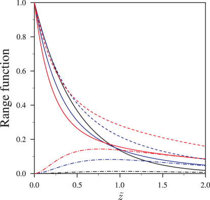
Figure 1: (Color online) The range functions of the charge and spin densities for the ordinary state, $g_{o}(z)$ (solid line) and $f(z)$ (dashed line), at given band parameter $\lambda=1.0$ (black line), $\lambda=2.0$ (blue lines), $\lambda=4.0$ (red lines). Note that at $\lambda=1.0$ the dependences $g_{o}(z)$ and $f(z)$ coincide. The range function of the topological state density, $g_{t}(z)$ (dotted-dashed line), at given band parameter $\lambda=1.1$ (black line), $\lambda=2.0$ (blue lines), $\lambda=4.0$ (red lines). $\widetilde{z}=z\sqrt{\frac{\Xi}{\mathrm{B}}}$ is the dimensionless coordinate.

IV TOPOLOGICAL BOUND STATE MODIFICATION

As said above, the contact between TI and topologically trivial insulator hosts, besides the ordinary bound state, the so-called topological bound state, which is specified by the Dirac spectrum and the envelope function $\{\Phi_{t}(\bm{\kappa},z),\Theta_{t}(\bm{\kappa},z)\}$. In the entire left half-space the envelope function is trivial, $\Phi_{t}(\bm{\kappa},z)=0$, in the right half-space it conforms to the conditions $\Theta_{t}(\bm{\kappa},z\rightarrow\infty)=0$ and $\Theta_{t}(\bm{\kappa},0+)=0$. Under these conditions the solution of the equation $[H_{t}^{0}(\bm{\kappa},-i\partial_{z})-E]\Theta(\bm{\kappa},z)=0$ (at $z>0$) has the form

$$\Theta_{t}^{0(\pm)}(\bm{\kappa},z) = C_{t}(\kappa)\Theta^{0(\pm)}(\phi)$$

$$\times \{\exp[-q_{1}(\kappa)z]-\exp[-q_{2}(\kappa)z]\},$$

where the spinor $\Theta^{0(\pm)}(\phi)=(i,sign(\mathrm{A}),\pm e^{i\phi},\pm sign(\mathrm{A})ie^{i\phi})^{\mathrm{T}}$ depends only on the polar angle of the momentum, $k_{\pm}=\kappa e^{\pm i\phi}$. The functions $\Theta_{t}^{0(+)}(\bm{\kappa},z)$ and $\Theta_{t}^{0(-)}(\bm{\kappa},z)$ describe the states with the positive $E_{t}^{0(+)}(\kappa)=|\mathrm{A}|\kappa$ and negative $E_{t}^{0(-)}(\kappa)=-|\mathrm{A}|\kappa$ energy, respectively; $C_{t}(\kappa)$ is the normalization factor.

By analogy with Eq. (31) one can to write the expression for the charge density in the unperturbed topological state (IV):

$$n_{t}(z)\simeq\frac{2a^{2}|C_{t}|^{2}}{\pi\mathrm{A}^{2}}(W^{2}+\mu^{2})g_{t}(z),$$ (36)

$$g_{t}(z)=\frac{1}{4}\biggl{\{}\exp[-q_{1}z]-\exp[-q_{2}z]\biggr{\}}^{2},$$ (37)

where $|C_{t}|^{2}=|\mathrm{A}|/8\mathrm{B}(\lambda-1)$. The spatial dependence (37) is given in Fig. 1. The topological state decays into the TI bulk on the length scale $z_{o}/2$, but the maximum of the density $n_{t}(z)$ does not occur at the interface, where $n_{t}(0)=0$, but rather near the point $z_{t}=\ln(q_{1}/q_{2})/(q_{1}-q_{2})$ ($z_{t}\lesssim\sqrt{\frac{\mathrm{B}}{\Xi}}<z_{o}$) on the TI side that is distant from the interface. Therefore, within our continual model, the topological state is directly insensitive to the local effective interface potential. Correspondingly, the direct magnetic coupling between the topological state and the FMI magnetization is absent since this state is spatially separated from the interface. Nevertheless, the topological state is subjected to the indirect influence of the interface with FMI through the extended fields $\varphi_{o}(z)$ and $\Delta_{o}(z)$ induced inside the TI host due to the orbital intermixing at the interface. We further show how the embedded exchange field $\Delta_{o}(z)$ affects the energy spectrum of the topological state.

Strictly speaking, we ought to find out an evanescent solution of the equation $[H_{t}(\bm{\kappa},-i\partial_{z})-E]\Theta(\bm{\kappa},z)=0$ at $z\rightarrow\infty$ and $z=0$, wherein the Hamiltonian operator (4) has the potential energy $\mathbb{U}=\varphi(z)\mathbb{I}+\tau_{0}\otimes(\bm{\sigma}\cdot\bm{\Delta}(z))$ with rather complicated matrix and spatial dependences. In the context of the magnetic proximity effect, we are interested to know how the induced exchange field $\Delta_{o}(z)$, applied along the $z$ axis, affects the electron spectrum of the topological state. Therefore we treat the potential energy $\mathbb{U}$ as a perturbation and remain only the exchange part $\mathbb{U}_{ex}(z)=\tau_{0}\otimes\sigma_{z}\Delta_{o}(z)$, where $\Delta_{o}(z)=\mathcal{K}s_{o}(z)$, the function $s_{o}(z)$ is given by Eqs. (33) and (III).

To estimate the modification of the topological state near the Dirac point under the exchange field, we utilize the method similar to the perturbation theory treatment for electron terms with close eigenenergies.Landau Indeed, near the Dirac point $\kappa=0$, there are energies in the spectrum of the unperturbed topological state, $E_{t}^{0(\pm)}(\kappa)=\pm|\mathrm{A}|\kappa$, the difference between which does not exceed the perturbation value $|\Delta_{o}(z)|$. For the perturbed envelope function $\Theta(\bm{\kappa},z)$ we employ the ansatz having the same spatial dependence of Eq. (IV), but the variable spinor structure $\Theta^{(\pm)}=(\theta_{1},\theta_{2},\theta_{3},\theta_{4})^{\mathrm{T}}$ that is driven by the perturbation. To seek for the factors $\theta_{j}$ we calculate the integral

$$\int_{0}^{\infty}dz\Theta^{{\dagger}}(\bm{\kappa},z)[H_{t}^{0}(\bm{\kappa},-i\partial_{z})+\mathbb{U}_{ex}(z)-E]\Theta(\bm{\kappa},z)=0.$$ (38)

The corresponding secular equation yields the spectrum of the topological state under the embedded exchange field:

$$E_{t}^{(\pm)}(\kappa)=\pm\sqrt{\mathrm{A}^{2}\kappa^{2}+I^{2}\Delta_{o}^{2}(0)},$$ (39)

where

$$I=\int_{0}^{\infty}dzf(z)[\Theta_{t}^{0(\pm)}(0,z)]^{{\dagger}}\mathbb{I}\Theta_{t}^{0(\pm)}(0,z)=\frac{1}{2}\frac{3\lambda-1}{3\lambda+1}.$$ (40)

The overlap integral $I$ is a function only of the material parameters of the TI bulk. The perturbation violates a parity between the minority and majority spin orientations of the electron states along the $z$ axis in accordance with

$$\Theta^{(\pm)}(\bm{\kappa}) \simeq \biggl{(}i,sign(\mathrm{A}),$$

$$\frac{e^{i\phi}|\mathrm{A}|\kappa}{E_{t}^{(\pm)}(\kappa)-I\Delta_{o}(0)},\frac{ie^{i\phi}\mathrm{A}\kappa}{E_{t}^{(\pm)}(\kappa)+I\Delta_{o}(0)}\biggr{)}^{\mathrm{T}}.$$

Ergo, the induced exchange field associated with the ordinary state penetrates into the TI host over distance on the order of $z_{o}/2$ to break the time reversal symmetry. As a consequence, the energy gap opens in the Dirac spectrum of the interface topological state $E_{t}^{(\pm)}(\kappa)$ (39). The gap size is directly proportional to the FMI magnetization and determined by the overlap of the ordinary state spin polarization and the topological state electron density, Eq. (40). As follows from Eqs. (20), (33) and (40), the induced gap size $2I\Delta_{o}(0)$ is limited by a number of factors: the intermixing intensity of the TI and FMI states at the interface, $Q$; the TI bulk band structure, $\lambda$; the Fermi level position, $\mu$, defining the TI states filling; and the exchange interaction strength in the TI bulk, $\mathcal{K}$.

The fact used in the present work is that the topological and ordinary states respond highly distinctly to the perturbation created by the TI/FMI interface. We show that the gap opens at the Dirac point of the topological state due to the exchange field originated from the spin polarized ordinary state. We conclude that the exchange coupling transfer through the mediation of the ordinary state is a key aspect of the mechanism of achieving interplay between FMI and the helical state in TI.

V SUMMARY AND CONCLUDING REMARKS

In this study, we have succeeded in understanding of the physical mechanism for magnetic proximity effect in the TI/FMI heterostructures, by using a rather simple model for both insulators and phenomenologically regarding the interface mixing between their states but ignoring the fine details of the interface on atomic scale. We have applied the envelope function method to study the in-gap bound states at the TI/FMI interface, wherein the narrow-gap semiconductor with inverted band structure is in the contact with the wide-gap magnetic semiconductor with normal band structure. Within the continual approach, to analytically describe the ordinary and topological interface states and interplay between them we have used the perturbation theory in the terms of the interface potential and the local approximation for an electron-electron interaction. It is no reason to think that there will be a qualitative difference with the obtained results when the self-consistent electrostatic and exchange fields are taken into account in the presence of an arbitrarily strong interface potential. Nevertheless the question about the electron density rearrangement within the interface region on the TI side is highly important to discuss it. It is particularly specific of the prototypical 3D TIs belonging to the Bi₂Se₃ family, which are narrow-gap semiconductors, that the screening scale is typically on the order of a quintuple thickness, i.e. $\approx$1 nm. It means that the fields $\varphi(\mathbf{r})$ and $\bm{\Delta}(\mathbf{r})$ figuring in Eq. (4), in strict sense, are neither long-range nor short-range fields. Therefore each of the limit treatments, the renormalization of the interface potential (that would be under the condition $D\ll z_{o}/2$) or the semiclassical treatment (that would be suited under the condition $D\gg z_{o}/2$), is the approximation for the fields $\varphi(\mathbf{r})$ and $\bm{\Delta}(\mathbf{r})$ that can yield only qualitative estimation for the spatial variation of electron density near the interface. To improve the description of the TI/FMI contact on the specific scale $D\approx z_{o}/2$, it should be reasonable one to utilize a fitting procedure with the sectionally continuous functions $\varphi(z)$ and $\Delta(z)$, for example, in the form of a rectangular or triangular potential well attached to the interface, where the value $\varphi(0)$ may, in principle, exceed the bulk energy gap and thus may significantly shift the energy spectrum $E_{o}^{\sigma}(\kappa)$ of the ordinary states relative to the bulk energy spectrum of TI. It is evident that such the modification of the model cannot change the principle conclusion about the mechanism of the magnetic proximity effect in the system under investigation.

An exchange field inside TI may also be induced by placing TI in contact with AFMI due to the presence of uncompensated magnetization in the outermost AFMI layer. The recent density functional theory (DFT) first-principles calculations for the Bi₂Se₃/MnSe superlattice expounded in Ref. Eremeev, has examined in detail the magnetic proximity effect near the 3D TI/AFMI (MnSe) interface. It was shown that the charge redistribution and mixing of the Bi₂Se₃ and MnSe orbitals at the interface brings on drastic modification of the electron structure with respect to the pristine Bi₂Se₃ surface. The calculation results reveal the presence of the ordinary state with probability maximum near the interface plane. This state penetrates into the first interfacial quintuple layer of TI. At the $\Gamma$ point, it appears in the local bulk valence band gap owing to the near-interface band bending of $\approx-0.8$ eV. This state is gapped (56 meV) and spin polarized due to the hybridization of the TI and AFMI states. On the other hand, the probability maximum of the Dirac topological state relocates from the first quintuple layer to the second one, leaving directly unattainable for a magnetic perturbation from MnSe. The interface ordinary state mediates an exchange coupling between AFMI and the topological state due to an overlap of the topological and trivial interface states within the first interfacial quintuple layer. The topological state acquires the energy gap of $\approx$8.5 meV proportional to the overlap.

The magnetic proximity effect in the TI/magnetic insulator (FMI or AFMI) hybrid structures is rather intricate phenomenon. The analytical continual model developed here and the DFT results of Ref. Eremeev, are in good qualitative agreement with each other. They unveil the unique route for the penetration of the exchange field into TI including three stages: the magnetic insulator magnetization $\rightarrow$ the interface ordinary state $\rightarrow$ the interface topological state.

It is likely that our results would be highly helpful for the analysis of the feasibility of recently proposed unusual physical effects in TIs and the “tailor-made” structures on their base, such as anomalous quantum Hall effect,Yu magnetic monopole imaging,Qi-09 topological contribution to the Faraday and Kerr effects,Qi-08 inverse spin-galvanic effect.Garate Our findings could provide guidelines to engineer spintronic device applications, for instance, the TI-based p-n junctionsWang and memory device based on the TI surface coated with a magnetic insulator film.Fujita

In summary, our analysis provides insight into the microscopic mechanism of the proximity effect in the TI/FMI hybrid structure. The nature of the proximity effect is tangled enough. The delicate moment is the presence of the ordinary state as a mediator for the spin polarization transmission over the interface from FMI to the topological state. We have distinguished way for modifying the spectrum of the topological state through the interface-induced exchange field that breaks time reversal symmetry, giving rise to the gap opening at the Dirac point in the topological state spectrum.

- (1) S. A. Wolf, D. D. Awschalom, R. A. Buhrman, J. M. Daughton, S. von Molnar, M. L. Roukes, A. Y. Chtchelkanova and D. M. Treger, Science 294, 1488 (2001).
- (2) I. Zutic, J. Fabian and S. Das Sarma, Rev. Mod. Phys. 76, 323 (2004).
- (3) R. Jansen, S. P. Dash, S. Sharma and B. C. Min, Semicond. Sci. Technol. 27, 083001 (2012).
- (4) V. N. Men’shov, V. V. Tugushev, S. Caprara, and E. V. Chulkov, Phys. Rev. B 81, 235212 (2010).
- (5) M. Z. Hasan and C. L. Kane, Rev. Mod. Phys. 82, 3045 (2010).
- (6) X. L. Qi and S. C. Zhang, Rev. Mod. Phys. 83, 1057 (2011).
- (7) I. Garate and M. Franz, Phys. Rev. Lett. 104, 146802 (2010).
- (8) Z. Zhou, Y. J. Chien, and C. Uher, Appl. Phys. Lett. 89, 232501 (2006).
- (9) A. Kandala, A. Richardella, D. W. Rench, D. M. Zhang, T. C. Flanagan, and N. Samarth, arXiv:1212.1225.
- (10) H. Ji, J. M. Allred, N. Ni, J. Tao, M. Neupane, A. Wray, S. Xu, M. Z. Hasan, and R. J. Cava, Phys. Rev. B 85, 165313 (2012).
- (11) P. Wei, F. Katmis, B. A. Assaf, H. Steinberg, P. Jarillo-Herrero, D. Heiman, and J. S. Moodera, Phys. Rev. Lett. 110, 186807 (2013).
- (12) W. Luo and X. L. Qi, Phys. Rev. B 87, 085431 (2013).
- (13) L. Fu, Phys. Rev. Lett. 103, 266801 (2009).
- (14) Y. Tserkovnyak and D. Loss, Phys. Rev. Lett. 108, 187201 (2012).
- (15) T. Yokoyama, J. Zang, and N. Nagaosa, Phys. Rev. B 81, 241410 (2010).
- (16) T. Habe, Y. Asano, Phys. Rev. B 85, 195325 (2012).
- (17) V. N. Men’shov, V. V. Tugushev, E. V. Chulkov, JETP Lett. 97, 258 (2013).
- (18) S.V. Eremeev, V. N. Men’shov, V. V. Tugushev, P. M. Echenique, and E. V. Chulkov, arXiv:1304.1275v1.
- (19) C. X. Liu, X. L. Qi, H. Zhang et al., Phys. Rev. B 82, 045122 (2010).
- (20) L. D. Landau and E. M. Lifshitz, Quntum Mechanics (Non-Relativistic Theory), Butterworth-Heinemann, Oxford, 1980.
- (21) R. Yu, W. Zhang, H. J. Zhang, S. C. Zhang, X. Dai, and Z. Fang, Science 329, 61 (2010).
- (22) X. L. Qi, R. Li, J. Zang, S. C. Zhang, Science 323, 1184 (2009).
- (23) X. L. Qi, T. L. Hughes, and S. C. Zhang, Phys. Rev. B 78, 195424 (2008).
- (24) J. Wang, X. Chen, B. F. Zhu, and S. C. Zhang, Phys. Rev. B 85, 235131 (2012).
- (25) T. Fujita, M. B. A. Jalil and S.G. Tan, Applied Physics Express 4, 094201 (2011).