Realistic Filter Cavities for Advanced Gravitational Wave Detectors

Abstract

The ongoing global effort to detect gravitational waves continues to push the limits of precision measurement while aiming to provide a new tool for understanding both astrophysics and fundamental physics. Squeezed states of light offer a proven means of increasing the sensitivity of gravitational wave detectors, potentially increasing the rate at which astrophysical sources are detected by more than an order of magnitude. Since radiation pressure noise plays an important role in advanced detectors, frequency dependent squeezing will be required. In this paper we propose a practical approach to producing frequency dependent squeezing for Advanced LIGO and similar interferometric gravitational wave detectors.

I Introduction

The Laser Interferometer Gravitational-Wave Observatory (LIGO) is part of a global effort to directly detect gravitational waves, which has the potential to revolutionize our understanding of both astrophysics, and fundamental physics.LIGO Laboratory (ment); Virgo Collaboration (ment); KAGRA (ment); GEO600 (ment) To realize this potential fully, however, significant improvements in sensitivity will be needed beyond Advanced LIGO and similar detectors.Harry and (2010) (The LIGO Scientific Collaboration); LIGO Scientific Collaboration (2010)

The use of squeezed states of light (known simply as “squeezing”) offers a promising direction for sensitivity improvement, and has the advantage of requiring minimal changes to the detectors currently under construction.LIGO Scientific Collaboration (2011); Barsotti (2013) Squeezing in advanced detectors will require that the squeezed state be varied as a function of frequency to suppress both the low-frequency radiation pressure noise and the high-frequency shot noise.Kimble et al. (2001); Chelkowski et al. (2005) When a squeezed state is reflected off a detuned optical cavity, the frequency-dependent amplitude and phase response of the cavity can be used to vary the squeezed state as a function of frequency. Though all future detectors plan to reduce quantum noise through squeezing, uncertainty remains with respect the practical design and limitations of the resonant optical cavities, known as “filter cavities”, this will require.McClelland et al. (2011); Khalili (2010)

In this paper we propose a practical approach to producing frequency dependent squeezing as required by advanced interferometric gravitational wave detectors. Section II describes the impact of squeezing and filter cavities in the context of a detector with realistic thermal noise, preparing us for a down-selection among filter cavity topologies. Section III goes on to suggest a filter cavity implementation appropriate for Advanced LIGO in light of realistic optical losses and other practical factors. Finally, in Appendix A we introduce a new approach to computing the quantum noise performance of interferometers with filter cavities in the presence of multiple sources of optical loss.

II Quantum Noise Filtering in Advanced Gravitational Wave Detectors

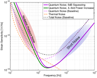
Figure 1: The sensitivity of an Advanced LIGO-like detector, our baseline (see table 1 for parameters), is limited at most frequencies by quantum noise, though at low frequencies thermal noise also contributes significantly. In terms of quantum noise, 6 dB of squeezing is equivalent to a 4-fold increase in power circulating in the interferometer, though always somewhat worse at low frequencies due to degradation of the squeezed vacuum state by optical losses and technical noises.Dwyer (2013) All of the curves in this paper assume $5\%$ injection loss (e.g., from the squeezed vacuum source to the interferometer), and $10\%$ readout loss (e.g., from the interferometer to the readout, including the photodetector quantum efficiency).

The quantum mechanical nature of light sets fundamental constraints on our ability to use it as a measurement tool, and in particular it produces a noise floor in interferometric position measurements like those employed by gravitational wave detectors. Figure 1 shows the expected sensitivity of an Advanced LIGO-like detector, in which quantum noise is dominant at essentially all frequencies (see Appendix A for calculation method and parameters).

The injection of a squeezed vacuum state into an interferometer can reduce quantum noise, as demonstrated in GEO600 and LIGO.LIGO Scientific Collaboration (2011); Barsotti (2013) The “frequency independent” form of squeezing used in these demonstrations will not, however, result in a uniform sensitivity improvement in an advanced detector. The difference comes from the expectation that radiation pressure noise will play a significant role in advanced detectors, and squeezing reduces shot noise at the expense of increased radiation pressure noise (see figure 1).

These demonstration experiments focused on reducing quantum noise at high frequency, where shot noise dominates, giving results similar to increasing the total power circulating in the detector (reduced shot noise and increased radiation pressure noise). Increasing circulating power, however, leads to significant technical difficulties related to thermal lensing and parametric instabilities.Evans, Barsotti, and Fritschel (2010); Harry and (2010) (The LIGO Scientific Collaboration) Furthermore, squeezing offers a means of reducing the quantum noise at any frequency simply by rotating the squeezed quadrature relative to the interferometer signal quadrature (known as the “squeeze angle”).Harms et al. (2003) In general, the squeeze angle that minimizes quantum noise varies as a function of frequency, and a technique for producing the optimal angle at all frequencies is required to make effective use of squeezing. One such technique is to reflect a frequency independent squeezed state off of a detuned Fabry-Perot cavity, known as a “filter cavity”.Kimble et al. (2001) Figure 2 shows a simplified interferometer with a squeezed light source and a filter cavity.

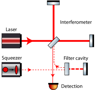
Figure 2: Frequency dependent squeezing can be produced with the help of a filter cavity. Shown here is a simplified interferometer with a linear “input filter cavity”.Kimble et al. (2001)

There are two primary options for the use of filter cavities to improve the sensitivity of advanced gravitational wave detectors; rotation of the squeezed vacuum state before it enters the interferometer, known as “input filtering”, and rotation of the signal and vacuum state as they exit the interferometer, known as “variational readout” or “output filtering”.Kimble et al. (2001); Harms et al. (2003); Khalili (2008) While variational readout appears to have great potential, a comprehensive study of input and output filtering in the presence of optical losses found that they result in essentially indistinguishable detector performance.Chen et al. (2010); McClelland et al. (2011); Khalili (2010)

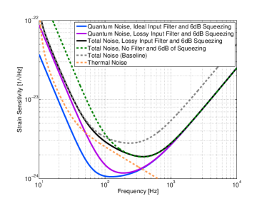
Figure 3: Frequency dependent squeezing decreases both shot noise and radiation pressure noise, reducing quantum noise at all frequencies (blue curve). A lossy filter cavity has degraded performance in the radiation pressure dominated region relative to an ideal lossless filter cavity (purple curve). The lossy filter shown here, with $1\text{\,}\mathrm{p}\mathrm{p}\mathrm{m}\mathrm{/}\mathrm{m}$ round-trip loss, represents a significant advantage over frequency independent squeezing in that it prevents an increase in radiation pressure noise (green dashed curve, see figure 1). Furthermore, since thermal noise is significant in the region where radiation pressure noise acts, there is little to be gained by making a lower loss filter cavity in the context of a near-term upgrade to Advanced LIGO.

III Filtering Solution for Advanced LIGO

In this section we propose a realistic filter cavity arrangement for implementation as an upgrade to Advanced LIGO. The elements of realism which drive this proposal are; the level of thermal noise and mode of operation expected in Advanced LIGO, the geometry of the Advanced LIGO vacuum envelope, and achievable values for optical losses in the squeezed field injection chain, in the filter cavity, and in the readout chain.

While frequency dependent squeezing for a general signal recycled interferometer requires two filter cavities, only one filter cavity is required to obtain virtually optimal results for a wide-band interferometer that is operated on resonance (i.e. in a “tuned” or “broadband” configuration).Purdue and Chen (2002); Khalili (2010) Since this is likely to be the primary operating state of Advanced LIGO we will start by restricting our analysis to this configuration.

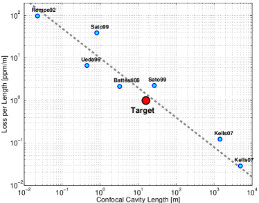
Figure 4: Measured round-trip loss per length from the literature.Rempe et al. (1992); Ueda et al. (1996); Sato et al. (1999); Kells (2007); Battesti et al. (2007) Losses grow with beam size on the optics, so a confocal geometry is optimal for minimizing losses and is a good choice for a filter cavity.Magaña-Sandoval et al. (2012) To remove any dependence on the choice of cavity geometry in the experiments presented here, the beam sizes on the optics are used to scale the cavity length to that of an equivalent confocal cavity. A rough fit to these data is included to guide the eye, and our target value of $1\text{\,}\mathrm{p}\mathrm{p}\mathrm{m}\mathrm{/}\mathrm{m}$ in a $16\text{\,}\mathrm{m}\text{/}$ cavity is marked.

Practically speaking, input filtering has the advantage of being functionally separate from the interferometer readout. That is, input filtering can be added to a functioning gravitational wave detector without modification, and even after it is added its use is elective. The same cannot be said for output filtering, which requires that a filter cavity be inserted into the interferometer’s readout chain. Furthermore, variational readout is incompatible with current DC readout schemes which produce a carrier field for homodyne detection by introducing a slight offset into the differential arm length, essentially requiring that the homodyne readout angle match the signal at DC, which is orthogonal to the angle required by variational readout.Kimble et al. (2001); Fricke et al. (2012); Evans (2013)

The essentially identical performance of input and output filtering, especially in the presence of realistic thermal noise, combined with the practical implications of both schemes push us to select a single input filter cavity as a the preferred option. That said, the requirements which drive input and output filter cavity design are very similar such that given a compatible readout scheme the input filter cavity solution presented here can also be used as an output filter cavity.

The impact of losses on cavity line-width is inversely proportional to cavity length, and thus it is always the loss per unit length that determines filter cavity performance.Khalili (2010) Figure 3 shows that less than 1 ppm/m round-trip loss will not significantly improve the detector’s sensitivity, so we take this as the target for an Advanced LIGO filter cavity. While this appears within reach given the optical losses reported in the literature (see figure 4), a study of optical losses in high finesse cavities as a function of cavity length with currently available polishing and coating technologies will be required to determine if this is realizable.

To achieve this loss target it is important to choose a filter cavity geometry which minimizes losses. A 2-mirror linear cavity with an isolator is a better choice than the 3-mirror triangular geometry frequently used to represent filter cavities,Kimble et al. (2001); Khalili (2007, 2010) since they both have essentially the same length while the linear cavity has fewer reflections and thus lower loss (see figure 5 for details).

Looking to a near-term upgrade of Advanced LIGO, the implementation of a short filter cavity which can be housed in the existing vacuum envelope will make squeezing a very attractive option. Since loss per unit length is observed to decrease with cavity length, it is advantageous to make a filter cavity as long as possible. The largest usable distance between two vacuum chambers that house the readout optics in the main experimental hall of Advanced LIGO is about $16\text{\,}\mathrm{m}\text{/}$ (see figure 6), which is plausibly sufficient to achieve the desired 1 ppm/m loss target.

Several technical issues in the implementation of a filter cavity for Advanced LIGO remain to be addressed before a precise performance prediction can be made. In addition to measurements of the dependence of optical loss on cavity length, the impact of spatial mode-mismatch and other sources of loss will need to be carefully evaluated. An analysis of technical noises which degrade filter cavity performance, especially via noise in the reflection phase of the filter cavity, will also be required.

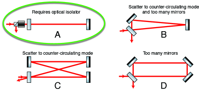
Figure 5: Various geometries considered for implementing a filter cavity. Factors considered in choosing among these geometries were: cavity length per mirror, potential for scatter into a counter-circulating mode, mode quality degradation due to large angle reflection from curved optics, and the ease of separating incident and reflected fields. While a linear cavity (option A) requires an optical isolator to separate input and output fields, it has the best length per mirror, no counter circulating mode, and good mode quality. A polarization based optical isolator is likely to introduce at least $1\%$ loss in the squeezed field injection. For short filter cavities, in which the separation between input and output beams is significant in a bow-tie geometry (C), the coupling to a counter-circulating mode may be negligible and the absence of an optical isolator will make this option preferable.

IV Conclusions

Squeezed vacuum states offer a proven means of enhancing the sensitivity of gravitational wave detectors, potentially increasing the rate at which astrophysical sources are detected by more than an order of magnitude.LIGO Scientific Collaboration (2011); Barsotti (2013) However, due to radiation pressure noise advanced detectors pose a more difficult problem than the proof-of-principle experiments conducted to date, and narrow line-width optical cavities will be required to make effective use of squeezing.

This work adds to previous efforts, which were aimed at parameterizing optimal filter cavity configurations in the context of a generalized interferometric gravitational wave detector, by identifying a practical and effective filter cavity design for Advanced LIGO and similar interferometric detectors. We find that a two-mirror linear cavity with $1\text{\,}\mathrm{p}\mathrm{p}\mathrm{m}\mathrm{/}\mathrm{m}$ round-trip loss is sufficient to reap the majority of the benefit that squeezing can provide.

Finally, we include a mathematical formalism which can be used to compute quantum noise in the presence of multiple sources of optical loss. This approach also maps the “audio sideband” or “one-photon” formalism commonly used to compute the behavior of classical fields in interferometers to the two-photon formalism used to compute quantum noise, thereby offering a simple connection between the optical parameters of a system and its quantum behavior.

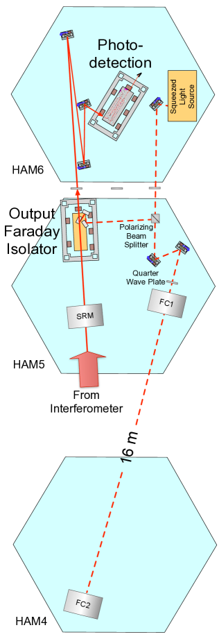
Figure 6: An input filter cavity could be included in the existing vacuum envelope of Advanced LIGO. The HAM4 and HAM5 chambers shown in this figure contain the interferometer output optics, and offer a $16\text{\,}\mathrm{m}\text{/}$ baseline with superior vibration isolation and direct access to the Faraday isolator with which squeezed vacuum will be injected. Acronyms used in the figure: signal recycling mirror (SRM), filter cavity input mirror (FC1), filter cavity end mirror (FC2).

Appendix A Mathematical Formalism

We use the following mathematical formalism to calculate quantum noise, as shown in figures 1 and 3. This treatment is based on Kimble et at.,Kimble et al. (2001) Buonanno and Chen,Buonanno and Chen (2001) and Harms et al.Harms et al. (2003) (hence forth KLMTV, BnC and HCF). The notation of HCF is used whenever possible.

This treatment extends HCF to a simple means of including all sources of loss, but makes no attempt to find analytic expressions for optimal values for filter cavity parameter as this appears better done numerically. To simplify the relevant expressions, a transformation from the one-photon formalism to the two-photon formalism is also presented, and utilized for computing the input-output relations of filter cavities.Caves and Schumaker (1985)

We start by noting that equation 2 in HCF can be written to express the output of the interferometer as a sum of signal and noise fields

$$\mathbf{\bar{o}}=\mathbf{\bar{s}}~{}h+\sum_{n}\mathbf{T_{n}}\mathbf{\bar{i}_{n}}$$ (1)

as suggested in the text preceding their equation 1. (The pre-factor $1/M$ in HCF is absorbed into $\mathbf{T_{n}}$ and $\mathbf{\bar{s}}$ to make them more independent.) In this notation each $\mathbf{\bar{i}_{n}}$ is a coherent vacuum field of the two-photon formalism such that

$$\mathbf{\bar{i}_{n}}=\begin{pmatrix}\alpha_{1}&\alpha_{2}\end{pmatrix},~{}\alpha_{1}=\begin{pmatrix}1\\ 0\end{pmatrix},~{}\alpha_{2}=\begin{pmatrix}0\\ 1\end{pmatrix}$$ (2)

where $\alpha_{1}$ and $\alpha_{2}$ represent the two field quadratures.Yuen (1976); Caves and Schumaker (1985) Thus, for $N$ vacuum fields entering an interferometer $\left\{\mathbf{\bar{i}_{1}},\dots,\mathbf{\bar{i}_{N}}\right\}$, there are $2N$ independent noise sources.

Carrying this through to the noise spectral density (HCF equation 7) gives

$$S_{h}=\frac{\sum_{n}\left|\mathbf{\bar{b}}_{\zeta}\cdot\mathbf{T_{n}}\right|^{2}}{\left|\mathbf{\bar{b}}_{\zeta}\cdot\mathbf{\bar{s}}\right|^{2}}$$ (3)

where we have kept the homodyne field vector $\mathbf{\bar{b}}_{\zeta}$ as in BnC. To avoid ambiguity: in our notation the dot product of vectors $\mathbf{\bar{a}}\cdot\mathbf{\bar{b}}\equiv\left<\mathbf{a}|\mathbf{b}\right>\equiv\sum_{n}a_{n}^{*}b_{n}$ is a complex number, the dot product of a vector and a matrix $\mathbf{\bar{a}}\cdot\mathbf{B}\equiv\left<\mathbf{a}\right|\mathbf{B}\equiv\mathbf{\bar{a}}^{\dagger}\mathbf{B}$ is a vector, and the magnitude squared of a vector $\left|\mathbf{\bar{a}}\right|^{2}\equiv\sum_{n}\left|a_{n}\right|^{2}$ is a real number.

In equation 3, each $\mathbf{T_{n}}$ is a $2\!\times\!2$ the transfer matrix which takes the coherent vacuum field $\mathbf{\bar{i}_{n}}$ from its point of entry into the interferometer to the readout photodetector. The transfer matrix $\mathbf{T_{1}}$ for vacuum fluctuations from the squeezed light source, for instance, can be constructed by taking a product of transfer matrices

$$\mathbf{T_{1}}=\mathbf{T_{ro}}\;\mathbf{T_{ifo}}\;\mathbf{T_{inj}}\;S(r,\lambda)$$ (4)

where $S(r,\lambda)$ is the operator for squeezing by $e^{r}$ with angle $\lambda$, $\mathbf{T_{inj}}$ takes the squeezed field from its source to the interferometer, $\mathbf{T_{ifo}}$ is the input-output transfer matrix of the interferometer ($\mathbf{C}/M$ in BnC, $\mathbf{T}/M$ in HCF), and $\mathbf{T_{ro}}$ transfers the field from the interferometer to the readout. In the case of input filtering $\mathbf{T_{inj}}$ will impose a frequency dependent rotation of the squeeze angle, while for output filtering $\mathbf{T_{ro}}$ will rotate the noise and signal fields as they propagate to the photodetector.

Computation of the input-output relation for any optical system can be performed in the two-photon formalism,Corbitt, Chen, and Mavalvala (2005) or in the simpler audio-sideband “one-photon” picture where the transfer of a field at frequency $\omega_{0}+\Omega$ is given by $\tau(\Omega)$ (as in previous works $\omega_{0}$ is the carrier frequency and $\Omega$ the signal sideband frequency). To convert between pictures we define transfer coefficients for positive and negative sidebands as $\tau_{+}=\tau(\Omega)$ and $\tau_{-}=\tau(-\Omega)$, and then compute the two-photon transfer matrix as

$$\mathbf{T}=A_{2}\begin{pmatrix}\tau_{+}&\\ &\tau^{*}_{-}\end{pmatrix}A_{2}^{-1},~{}A_{2}=\frac{1}{\sqrt{2}}\begin{pmatrix}1&1\\ -i&+i\end{pmatrix}~{}.$$ (5)

Off-diagonal elements in the one-photon transfer matrix are unnecessary for filter cavities, since those elements represent non-linear transformations that couple the positive and negative sideband amplitudes such as squeezing or radiation pressure back-action.

For a filter cavity, the one-photon transfer coefficient is just the amplitude reflectivity of the cavity

$$r_{fc}(\Omega)=r_{in}-\frac{t_{in}^{2}}{r_{in}}\;\frac{r_{rt}e^{-i\phi(\Omega)}}{1-r_{rt}e^{-i\phi(\Omega)}}$$ (6)

where the cavity round-trip reflectivity $r_{rt}$ is related to its bandwidth by

$$\gamma_{fc}=-\log(r_{rt})\;f_{FSR}\simeq\frac{1-r_{rt}^{2}}{2}f_{FSR},\quad f_{FSR}=\frac{c}{2L_{fc}}$$ (7)

and the round-trip phase derives from the cavity detuning according to

$$\phi(\Omega)=\frac{\Omega-\Delta\omega_{fc}}{f_{FSR}},\quad\Delta\omega_{fc}=\omega_{fc}-\omega_{0}$$ (8)

for a cavity of length $L_{fc}$ and resonant frequency $\omega_{fc}$. (The cavity “bandwidth” is the half-width of the resonance, a.k.a. the “cavity pole” frequency. In KLMTV the detuning is given in terms of the bandwidth $\xi=\Delta\omega_{fc}/\gamma_{fc}$.) The amplitude reflectivity of the cavity input-output coupler is related to its transmissivity by $r_{in}^{2}\leq 1-t_{in}^{2}$, and to the round-trip reflectivity by $r_{rt}\leq r_{in}$, where a lossless filter cavity attains equality in both expressions. The filter cavity transfer matrix in the two-photon formalism is

$$\mathbf{T_{fc}}=A_{2}\begin{pmatrix}r_{fc+}&\\ &r^{*}_{fc-}\end{pmatrix}A_{2}^{-1}.$$ (9)

Returning to an interferometer with input filtering, and including injection and readout losses, we can write

$$\mathbf{\bar{s}} = L(\Lambda_{ro})\;\mathbf{\bar{s}}_{0}$$ (10)

$$\mathbf{T_{in1}} = L(\Lambda_{ro})\;\mathbf{T_{ifo}}\;\mathbf{T_{fc}}\;L(\Lambda_{inj})\;S(r,\lambda)$$ (11)

$$\mathbf{T_{in2}} = L(\Lambda_{ro})\;\mathbf{T_{ifo}}\;\mathbf{T_{fc}}\;\Lambda_{inj}$$ (12)

$$\mathbf{T_{in3}} = L(\Lambda_{ro})\;\mathbf{T_{ifo}}\;\Lambda_{fc}$$ (13)

$$\mathbf{T_{in4}} = \Lambda_{ro}$$ (14)

where $L(\Lambda_{x})=\sqrt{1-\Lambda_{x}^{2}}$ is the transfer coefficient of a power loss $\Lambda_{x}^{2}$. The four $\mathbf{T_{n}}$ terms each contribute to the sum in equation 3, since each represents an entry point for coherent vacuum fluctuations.Kimble et al. (2001) $\mathbf{T_{in1}}$ propagates the squeezed field from its source to the photodetector, and $\mathbf{T_{in2}}$ accounts for the losses of the injection path (from squeezer to filter cavity). $\mathbf{T_{in3}}$ represents the frequency dependent losses in the filter cavity with

$$\Lambda_{fc}^{2}=1-(\left|r_{fc+}\right|^{2}+\left|r_{fc-}\right|^{2})/2\quad.$$ (15)

Finally, $\mathbf{T_{in4}}$ accounts for losses in the readout path, from interferometer to photodetector including the detector quantum efficiency.

For an interferometer with output filtering, on the other hand, we have

$$\mathbf{\bar{s}} = L(\Lambda_{ro})\;\mathbf{T_{fc}}\;\mathbf{\bar{s}}_{0}$$ (16)

$$\mathbf{T_{out1}} = L(\Lambda_{ro})\;\mathbf{T_{fc}}\;\mathbf{T_{ifo}}\;L(\Lambda_{inj})\;S(r,\lambda)$$ (17)

$$\mathbf{T_{out2}} = L(\Lambda_{ro})\;\mathbf{T_{fc}}\;\mathbf{T_{ifo}}\;\Lambda_{inj}$$ (18)

$$\mathbf{T_{out3}} = L(\Lambda_{ro})\;\Lambda_{fc}$$ (19)

$$\mathbf{T_{out4}} = \Lambda_{ro}$$ (20)

where the signal produced by the interferometer $\mathbf{\bar{s}}_{0}$ is modified by the filter cavity, in addition to experiencing some loss in the readout process.

The transfer matrix and signal vector for a tuned signal recycled interferometer of the sort discussed in section III and analyzed in III.C.2 of BnC, are

$$\mathbf{T_{ifo}}=\begin{pmatrix}1&\mathcal{K}_{sr}\\ 0&1\end{pmatrix},~{}\mathbf{\bar{s}}_{0}=\frac{\sqrt{2\mathcal{K}_{sr}}}{h_{SQL}}\begin{pmatrix}1\\ 0\end{pmatrix},~{}$$ (21)

where

$$h_{SQL}=\sqrt{\frac{8\hbar}{mL_{arm}^{2}\Omega^{2}}},\quad\mathcal{K}_{sr}=\frac{\mathcal{K}\;t_{sr}^{2}}{\left|1+e^{2i\Phi}r_{sr}\right|^{2}},$$ (22)

$$\mathcal{K}=\frac{8P_{bs}\;\omega_{0}}{mL_{arm}^{2}\Omega^{2}(\Omega^{2}+\gamma_{arm}^{2})},$$ (23)

$$\Phi=\Omega L_{src}/c+\,{\textrm{arctan}}\!\left({\Omega/\gamma_{arm}}\right),$$ (24)

and the signal recycling mirror amplitude reflectivity and transmissivity are $r_{sr}$ and $t_{sr}$ for consistency with equations 6-9 (these are $\rho$ and $\tau$ in BnC and HCF). (There appear to be several errors in HCF with respect to the equations for Advanced LIGO, making BnC a better reference.) Symbol definitions, and the values used in our calculations, are given in table 1.

Table 1: Symbols and values

Symbol	Meaning	Value
$c$	light speed	$299\,792\,458\text{\,}\mathrm{m}\mathrm{/}\mathrm{s}$
$\omega_{0}$	frequency of carrier field	$2\pi\times$282\text{\,}\mathrm{THz}\text{/}$$
$P_{bs}$	power on the beam-splitter	$5.6\text{\,}\mathrm{kW}\text{/}$
$m$	mass of each test-mass mirror	$40\text{\,}\mathrm{kg}\text{/}$
$L_{arm}$	arm cavity length	$3995\text{\,}\mathrm{m}\text{/}$
$L_{src}$	signal cavity length	$55\text{\,}\mathrm{m}\text{/}$
$\gamma_{arm}$	arm cavity half-width	$2\pi\times$42\text{\,}\mathrm{Hz}\text{/}$$
$t_{sr}^{2}$	signal mirror power transmission	$35\%$
$\Lambda_{inj}^{2}$	injection losses	$5\%$
$\Lambda_{ro}^{2}$	readout losses	$10\%$
$t_{in}^{2}$	filter cavity input transmission
	ideal $16\text{\,}\mathrm{m}\text{/}$ filter cavity	$66\text{\,}\mathrm{p}\mathrm{p}\mathrm{m}$
	$1\text{\,}\mathrm{p}\mathrm{p}\mathrm{m}\mathrm{/}\mathrm{m}$ loss $16\text{\,}\mathrm{m}\text{/}$ filter cavity	$50\text{\,}\mathrm{p}\mathrm{p}\mathrm{m}$
$\gamma_{fc}$	filter cavity half-width	$2\pi\times$49\text{\,}\mathrm{Hz}\text{/}$$
$\Delta\omega_{fc}$	filter cavity detuning	$2\pi\times$49\text{\,}\mathrm{Hz}\text{/}$$

References

- LIGO Laboratory (ment) LIGO Laboratory, “LIGO web site,” (living document).
- Virgo Collaboration (ment) Virgo Collaboration, “Virgo web site,” (living document).
- KAGRA (ment) KAGRA, “KAGRA web site,” (living document).
- GEO600 (ment) GEO600, “GEO web site,” (living document).
- Harry and (2010) (The LIGO Scientific Collaboration) G. M. Harry and (The LIGO Scientific Collaboration), “Advanced LIGO: the next generation of gravitational wave detectors,” Classical and Quantum Gravity 27, 084006 (2010).
- LIGO Scientific Collaboration (2010) LIGO Scientific Collaboration, “GWIC Roadmap,” (2010).
- LIGO Scientific Collaboration (2011) LIGO Scientific Collaboration, “A gravitational wave observatory operating beyond the quantum shot-noise limit,” Nature Physics 7, 962–965 (2011).
- Barsotti (2013) L. Barsotti, “Enhancing the astrophysical reach of the LIGO gravitational wave detector by using squeezed states of light,” (2013), in Preparation.
- Kimble et al. (2001) H. Kimble, Y. Levin, A. Matsko, K. Thorne, and S. Vyatchanin, “Conversion of conventional gravitational-wave interferometers into quantum nondemolition interferometers by modifying their input and/or output optics,” Physical Review D 65 (2001).
- Chelkowski et al. (2005) S. Chelkowski, H. Vahlbruch, B. Hage, A. Franzen, N. Lastzka, K. Danzmann, and R. Schnabel, “Experimental characterization of frequency-dependent squeezed light,” Physical Review A 71 (2005).
- McClelland et al. (2011) D. McClelland, N. Mavalvala, Y. Chen, and R. Schnabel, “Advanced interferometry, quantum optics and optomechanics in gravitational wave detectors,” Laser & Photonics Reviews , 677–696 (2011).
- Khalili (2010) F. Y. Khalili, “Optimal configurations of filter cavity in future gravitational-wave detectors,” Physical Review D 81, 122002 (2010).
- Evans, Barsotti, and Fritschel (2010) M. Evans, L. Barsotti, and P. Fritschel, “A general approach to optomechanical parametric instabilities,” Physics Letters A 374, 665–671 (2010).
- Dwyer (2013) S. Dwyer, “Squeezing angle fluctuations in a quantum enhanced gravitational wave detector,” (2013), in Preparation.
- Harms et al. (2003) J. Harms, Y. Chen, S. Chelkowski, A. Franzen, H. Vahlbruch, K. Danzmann, and R. Schnabel, “Squeezed-input, optical-spring, signal-recycled gravitational-wave detectors,” Physical Review D 68, 042001 (2003).
- Khalili (2008) F. Khalili, “Increasing future gravitational-wave detectors’ sensitivity by means of amplitude filter cavities and quantum entanglement,” Physical Review D 77, 062003 (2008).
- Chen et al. (2010) Y. Chen, S. L. Danilishin, F. Y. Khalili, and H. Müller-Ebhardt, “QND measurements for future gravitational-wave detectors,” General Relativity and Gravitation 43, 671–694 (2010).
- Purdue and Chen (2002) P. Purdue and Y. Chen, “Practical speed meter designs for quantum nondemolition gravitational-wave interferometers,” Physical Review D 66 (2002).
- Fricke et al. (2012) T. T. Fricke, N. D. Smith-Lefebvre, R. Abbott, R. Adhikari, K. L. Dooley, M. Evans, P. Fritschel, V. V. Frolov, K. Kawabe, J. S. Kissel, B. J. J. Slagmolen, and S. J. Waldman, “DC readout experiment in Enhanced LIGO,” Classical and Quantum Gravity 29, 065005 (2012).
- Evans (2013) M. Evans, “Low-Noise Homodyne Readout for Quantum Limited Gravitational Wave Detectors,” (2013), in Preparation.
- Khalili (2007) F. Khalili, “Quantum variational measurement in the next generation gravitational-wave detectors,” Physical Review D 76, 102002 (2007).
- Rempe et al. (1992) G. Rempe, R. J. Thompson, H. J. Kimble, and R. Lalezari, “Optics InfoBase: Optics Letters - Measurement of ultralow losses in an optical interferometer,” Optics letters (1992).
- Ueda et al. (1996) A. Ueda, N. Uehara, K. Uchisawa, K.-i. Ueda, H. Sekiguchi, T. Mitake, K. Nakamura, N. Kitajima, and I. Kataoka, “Ultra-High Quality Cavity with 1.5 ppm Loss at 1064 nm,” Optical Review 3, 369–372 (1996).
- Sato et al. (1999) S. Sato, S. Miyoki, M. Ohashi, and M. K. Fujimoto, “Optics InfoBase: Applied Optics - Loss Factors of Mirrors for a gravitational wave Antenna,” Applied … (1999).
- Kells (2007) W. Kells, “Initial LIGO COC Loss investigation Summary,” Tech. Rep. LIGO-T070051 (CALIFORNIA INSTITUTE OF TECHNOLOGY, 2007) https://dcc.ligo.org/LIGO-T070051.
- Battesti et al. (2007) R. Battesti, B. Pinto Da Souza, S. Batut, C. Robilliard, G. Bailly, C. Michel, M. Nardone, L. Pinard, O. Portugall, G. Trénec, J. M. Mackowski, G. L. J. A. Rikken, J. Vigué, and C. Rizzo, “The BMV experiment: a novel apparatus to study the propagation of light in a transverse magnetic field,” The European Physical Journal D 46, 323–333 (2007).
- Magaña-Sandoval et al. (2012) F. Magaña-Sandoval, R. X. Adhikari, V. Frolov, J. Harms, J. Lee, S. Sankar, P. R. Saulson, and J. R. Smith, “Large-angle scattered light measurements for quantum-noise filter cavity design studies,” JOSA A 29, 1722–1727 (2012).
- Buonanno and Chen (2001) A. Buonanno and Y. Chen, “Quantum noise in second generation, signal-recycled laser interferometric gravitational-wave detectors,” Phys. Rev. D 64, 042006 (2001).
- Caves and Schumaker (1985) C. M. Caves and B. L. Schumaker, “New formalism for two-photon quantum optics. I. Quadrature phases and squeezed states,” Physical Review A 31, 3068 (1985).
- Yuen (1976) H. Yuen, “Two photon coherent states of the radiation field,” Phys.Rev. A13, 2226–2243 (1976).
- Corbitt, Chen, and Mavalvala (2005) T. Corbitt, Y. Chen, and N. Mavalvala, “Mathematical framework for simulation of quantum fields in complex interferometers using the two-photon formalism,” Physical Review A 72 (2005).