The scattering map in two coupled piecewise-smooth systems, with numerical application to rocking blocks

Abstract

We consider a non-autonomous dynamical system formed by coupling two piecewise-smooth systems in $\mathbb{R}^{2}$ through a non-autonomous periodic perturbation. We study the dynamics around one of the heteroclinic orbits of one of the piecewise-smooth systems. In the unperturbed case, the system possesses two $C^{0}$ normally hyperbolic invariant manifolds of dimension two with a couple of three dimensional heteroclinic manifolds between them. These heteroclinic manifolds are foliated by heteroclinic connections between $C^{0}$ tori located at the same energy levels. By means of the impact map we prove the persistence of these objects under perturbation. In addition, we provide sufficient conditions of the existence of transversal heteroclinic intersections through the existence of simple zeros of Melnikov-like functions. The heteroclinic manifolds allow us to define the scattering map, which links asymptotic dynamics in the invariant manifolds through heteroclinic connections. First order properties of this map provide sufficient conditions for the asymptotic dynamics to be located in different energy levels in the perturbed invariant manifolds. Hence we have an essential tool for the construction of a heteroclinic skeleton which, when followed, can lead to the existence of Arnol’d diffusion: trajectories that, on large time scales, destabilize the system by further accumulating energy. We validate all the theoretical results with detailed numerical computations of a mechanical system with impacts, formed by the linkage of two rocking blocks with a spring.

1 Introduction

This paper is concerned with the question of whether it is possible to observe Arnol’d diffusion [Arn64] in systems governed by piecewise-smooth differential equations, to which known results in the field can not be directly applied. Arnol’d diffusion occurs when there is a large change in the action variables in nearly integrable Hamiltonian systems. Systems governed by piecewise-smooth differential equations are widespread in engineering, economics, electronics, ecology and biology; see [ML12] for a recent comprehensive survey of the field.

Action variables are conserved for integrable systems. When such systems are perturbed, for example, by a periodic forcing, KAM theory tells us that the value of these variables stays close to their conserved values for most solutions. Subsequently Arnol’d [Arn64] gave an example of an nearly integrable system for which there was large growth in the action variables.

There has been a lot of activity in the field of Arnol’d diffusion in recent years and a large variety of results that have been obtained or announced. We refer to [DGdlLS08, Che08, Che10, Ber10] for a detailed survey of recent results. Up to now, there are mainly two kind of methods used to prove the existence of instabilities in Hamiltonian systems close to integrable; variational methods [Ber02, BBB02, BBB03, Mat02, CY04, KL08b, KL08a, BKZ11, KZ12] and the so-called geometric methods [DdlLS00, DdlLS06, DdlLS08, GdlL06, Tre04, Tre12, FGKR11], both of which have been used to prove generic results or study concrete examples.

The study of Arnol’d diffusion using geometric methods has been greatly facilitated by the introduction [DdlLS00, DdlLS06, DdlLS08] of the scattering map of a normally hyperbolic invariant manifold with intersecting stable and unstable invariant manifolds along a homoclinic manifold. This map finds the asymptotic orbit in the future, given an asymptotic orbit in the past. Perturbation theory of the scattering map [DdlLS08] generalizes and extends several results obtained using Melnikov’s method [Mel63, GH83].

For planar regular systems under non-autonomous periodic perturbations, Melnikov’s method is used to determine the persistence of periodic orbits and homoclinic/heteroclinic connections by guaranteeing the existence of simple zeros of the subharmonic Melnikov function and the Melnikov function, respectively. The main idea is to consider a section normal to the unperturbed vector field at some point on the unperturbed homoclinic/heteroclinic connection. Then it is possible to measure the distance between the perturbed manifolds, owing to the regularity properties of the stable and unstable manifolds of hyperbolic critical points in smooth systems.

In [GHS12] these classical results were rigorously extended to a general class of piecewise-smooth differential equations, allowing for a general periodic Hamiltonian perturbation, with no symmetry assumptions. For such systems, the unperturbed system is defined in two domains, separated by a switching manifold $\Sigma$, each possessing one hyperbolic critical point either side of $\Sigma$. In this case, the vector normal to the unperturbed vector field is not defined everywhere. By looking for the intersection between the stable and unstable manifolds with the switching manifold, an asymptotic formula for the distance between the manifolds was obtained. This turned out to be a modified Melnikov function, whose zeros give rise to the existence of heteroclinic connections for the perturbed system. The general results in [GHS12] were then applied to the case of the rocking block [Hou63, Hog89] and excellent agreement was obtained with the results of  [Hog89].

Following these ideas, in this paper we study a system which consists of a non-autonomous periodic perturbation of a piecewise-smooth integrable Hamiltonian system in $\mathbb{R}^{4}$. The unperturbed system is given by the product of two piecewise-smooth systems. We assume that one of them has two hyperbolic critical points of saddle type with a pair of $C^{0}$ heteroclinic orbits between them. The other system behaves as a classical integrable system with a region foliated by $C^{0}$ periodic orbits. Therefore, the product system looks like a classical a priori unstable Hamiltonian system [CG94], possessing two $C^{0}$ normally hyperbolic invariant manifolds of dimension two with a couple of three dimensional $C^{0}$ heteroclinic manifolds.

The main difficulty in following the program of [DdlLS06] is that we couple two piecewise-smooth systems, each of which possesses its own switching manifold. Therefore, when considering the product system, we need to deal with a piecewise-smooth system in $\mathbb{R}^{4}$ with two 3-dimensional switching manifolds that cross in a 2-dimensional one. Therefore the classical impact map associated with one switching manifold will be piecewise-smooth in general. We overcome this difficulty by restricting the impact map to suitable domains so that we can apply classical results for normally hyperbolic invariant manifolds and their persistence and obtain a scattering map between them with explicit asymptotic formulae.

Note that, in this paper, we restrict our attention to the study of the scattering map and we do not rigorously prove the existence of Arnol’d diffusion. Due to the continuous nature of the system considered in this paper, the method of correctly aligned windows [GdlL06] seems to be very suitable for application to our model for this purpose. In fact, recent results in [RdlL02], which do not rely on the use of KAM theory, appear to be capable of extension to piecewise-smooth systems in order to achieve this goal.

Piecewise-smooth systems are found in a host of applications [ML12]. A simple example is the rocking block model [Hou63], which has wide application in earthquake engineering and robotics. This piecewise-smooth system has been shown to possess a vast array of solutions [Hog89]. The model has been extended to include, for example, stacked rigid blocks [SRP01] and multi–block structures [PLC08]. Particular attention is paid to the case of block overturning in the presence of an earthquake, as this has consequences for safety in the nuclear industry [CK09] and for the preservation of ancient statues [KPC12]. Within the context of the current paper, Arnol’d diffusion could be seen as one possible mechanism for block overturning, when the perturbation (earthquake) of an apparently stable system (two blocks coupled by a simple spring) leads to overturning. An early application of Melnikov theory to the rocking block problem [Kov10] involved the calculation of the stochastic Melnikov criterion of instability for a multidimensional rocking structure subjected to random excitation.

Note that we are considering the class of piecewise-smooth differential equations that involve crossing [ML12], where the normal components of the vector field either side of the switching manifold are in the same sense. When these components are in the opposite sense, sliding can occur [ML12]. The extension of the Melnikov method to this case is still in its infancy [DuLi12].

The paper is organised as follows. In section 2 we present the system we will consider and the main piecewise-smooth invariant geometrical objects that will play a role in the process. In section 3 we present the impact map associated with one switching manifold in the extended phase space and its domains of regularity and provide an explicit expression for it in the unperturbed case. In section 4 we study some regular normally hyperbolic invariant manifolds for the impact map which correspond to the piecewise-smooth ones for the flow in the extended phase space. We then apply classical perturbation theory to demonstrate the persistence of the normally hyperbolic invariant manifolds and their stable and unstable manifolds and deduce the persistence of the corresponding invariant manifolds for the perturbed flow. This allows us to give explicit conditions for the existence of transversal heteroclinic manifolds in the perturbed system in terms of a modified Melnikov function and to derive explicit formulae for the scattering map in section 5. In particular, we obtain formulae for the change in the energy of the points related by the scattering map and in the average energy along their orbits. In section 6 we illustrate the theoretical results of section 5 with numerical computations for two coupled rocking blocks subjected to a small periodic forcing. We use the simple zeros of the Melnikov function to numerically compute heteroclinic connections linking, forwards and backwards in time, two trajectories at the invariant manifolds. These trajectories correspond to one block performing small rocking oscillations while the other block rocks about one of its heteroclinic orbits. During this large, fast, excursion, the amplitude of the rocking block oscillations may lead to an increase or decrease in its average energy. Using the first order analysis of the scattering map we are able to approximately predict the magnitude of this change, which is in excellent agreement with our numerical computations.

2 System description

2.1 Two uncoupled systems

In this paper we consider a non-autonomous dynamical system formed by coupling two piecewise-smooth systems in $\mathbb{R}^{2}$ through a non-autonomous periodic perturbation. We divide $\mathbb{R}^{2}$ into two sets,

$$S^{+}=\left\{(q,p)\in\mathbb{R}^{2}\,|\,q>0\right\},$$

$$S^{-}=\left\{(q,p)\in\mathbb{R}^{2}\,|\,q<0\right\},$$

separated by the switching manifold

$$\Sigma=\Sigma^{+}\cup\Sigma^{-}\cup\{(0,0)\},$$ (2.1)

where

$$\Sigma^{+}=\left\{(0,p)\in\mathbb{R}^{2}\,|\,p>0\right\},$$ (2.2)

$$\Sigma^{-}=\left\{(0,p)\in\mathbb{R}^{2}\,|\,p<0\right\}.$$

We consider the piecewise-smooth systems defined in $\mathbb{R}^{2}\backslash\Sigma$

$$\left(\begin{array}[]{c}\dot{x}\\ \dot{y}\end{array}\right):=\mathcal{X}(x,y):=\left\{\begin{aligned} &\mathcal{X}^{+}(x,y)&&\text{if }(x,y)\in S^{+}\\ &\mathcal{X}^{-}(x,y)&&\text{if }(x,y)\in S^{-}\end{aligned}\right.$$ (2.3)

$$\left(\begin{array}[]{c}\dot{u}\\ \dot{v}\end{array}\right):=\mathcal{U}(u,v):=\left\{\begin{aligned} &\mathcal{U}^{+}(u,v)&&\text{if }(u,v)\in S^{+}\\ &\mathcal{U}^{-}(u,v)&&\text{if }(u,v)\in S^{-}\end{aligned}\right.$$ (2.4)

with $\mathcal{X}^{\pm}(x,y),\,\mathcal{U}^{\pm}(u,v)\in C^{\infty}(\mathbb{R}^{2})$.

Let us assume that (2.3) and (2.4) are Hamiltonian systems associated, respectively, with $C^{0}(\mathbb{R}^{2})$ piecewise-smooth Hamiltonians of the form

$$X(x,y) :=\frac{y^{2}}{2}+Y(x)$$

$$:=\left\{\begin{aligned} &X^{+}(x,y):=\frac{y^{2}}{2}+Y^{+}(x)&&\text{if }(x,y)\in S^{+}\\ &X^{-}(x,y):=\frac{y^{2}}{2}+Y^{-}(x)&&\text{if }(x,y)\in S^{-}\end{aligned}\right.$$ (2.5)

$$U(u,v) :=\frac{v^{2}}{2}+V(u)$$

$$:=\left\{\begin{aligned} &U^{+}(u,v):=\frac{v^{2}}{2}+V^{+}(u)&&\text{if }(u,v)\in S^{+}\\ &U^{-}(u,v):=\frac{v^{2}}{2}+V^{-}(u)&&\text{if }(u,v)\in S^{-},\end{aligned}\right.$$ (2.6)

with $Y^{\pm},\,V^{\pm}\in C^{\infty}(\mathbb{R}^{2})$ satisfying $Y^{+}(0)=Y^{-}(0)=0$ and $V^{+}(0)=V^{-}(0)=0$. Then

$$\mathcal{X}^{\pm} =J\nabla X^{\pm}$$ (2.7)

$$\mathcal{U}^{\pm} =J\nabla U^{\pm}$$

where $J$ is the symplectic matrix

$$J=\left(\begin{array}[]{cc}0&1\\ -1&0\end{array}\right).$$

From the form of the Hamiltonians (2.5) and (2.6), it is natural to extend the definition of the flows of $\mathcal{X}^{+}$ and $\mathcal{U}^{+}$ to $S^{+}\cap\Sigma^{+}$ and of the flows of $\mathcal{X}^{-}$ and $\mathcal{U}^{-}$ to $S^{-}\cap\Sigma^{-}$. Hence, the Hamiltonian $X(x,y)$ in (2.5) is naturally extended to $\mathbb{R}^{2}$ as

$$X(x,y)=\left\{\begin{aligned} &X^{+}(x,y)&&\text{if }(x,y)\in S^{+}\cup\Sigma^{+}\cup\left\{(0,0)\right\}\\ &X^{-}(x,y)&&\text{if }(x,y)\in S^{-}\cup\Sigma^{-},\end{aligned}\right.$$

and similarly for the Hamiltonian $U(u,v)$ in (2.6). Note that the vector fields $\mathcal{X}^{+}$ and $\mathcal{X}^{-}$ are tangent to $\Sigma$ at $(0,0)$ (resp. $\mathcal{U}^{+}$ and $\mathcal{U}^{-}$).

To define the flow associated with system (2.3), we proceed as usual in piecewise-smooth systems. Given an initial condition $(x_{0},y_{0})\in S^{\pm}$, we apply the flows $\phi_{\mathcal{X}^{\pm}}$ associated with the smooth systems $\mathcal{X}^{\pm}$ until the switching manifold $\Sigma$ is crossed at some point. Then, using this point as the new initial condition we evolve with the flow in the new domain. The flow associated with system (2.4) is defined in a similar way. Note that, as no sliding along the switching manifold is possible, the definition of the flows is straightforward. This allows us to consider the flows

$$\phi_{\mathcal{X}}(t;x_{0},y_{0})\text{ and }\phi_{\mathcal{U}}(t;,u_{0},v_{0})$$ (2.8)

associated with systems (2.3) and (2.4), respectively, that are $C^{0}$ functions piecewise-smooth in $t$ satisfying

$$\phi_{\mathcal{X}}(0;,x_{0},y_{0}) =(x_{0},y_{0})$$

$$\phi_{\mathcal{U}}(0;,u_{0},v_{0}) =(u_{0},v_{0}).$$

Let us assume that the following conditions are satisfied.

1. System (2.3) possesses two hyperbolic critical points $Q^{+}\in S^{+}$ and $Q^{-}\in S^{-}$ of saddle type belonging to the energy level $X(x,y)=\bar{d}$.

2. The energy level $X(x,y)=\bar{d}$ contains two heteroclinic orbits given by $\gamma^{\text{up}}:=W^{u}(Q^{-})=W^{s}(Q^{+})$ and $\gamma^{\text{down}}:=W^{u}(Q^{+})=W^{s}(Q^{-})$.

3. The Hamiltonians $U^{\pm}$ in (2.6) satisfy

   $$(V^{+})^{\prime}(0)>0;\;(V^{-})^{\prime}(0)<0,$$

   and so $(0,0)$ is an invisible quadratic tangency for both vector fields $\mathcal{U}^{\pm}$ in (2.4). Following [Kuz04, GST11], we call the point $(0,0)$ an invisible fold-fold.

4. System (2.4) possesses a continuum of (piecewise-smooth) continuous periodic orbits surrounding the origin. These can be parameterized by the Hamiltonian $U$ and have the form

   $$\Lambda_{c}=\left\{(u,v)\in\mathbb{R}^{2}\,|\,U(u,v)=c\right\},\;0<c\leq\bar{c}.$$ (2.9)

The main purpose of this paper is to study the dynamics around one of the heteroclinic orbits of system (2.3). From now on, we focus on the upper one

$$\gamma^{\text{up}}:=W^{u}(Q^{-})\cap W^{s}(Q^{+})=\left\{(x,y)\in\mathbb{R}^{2}\,|\,X(x,y)=\bar{d},\,y\geq 0\right\}.$$

There we consider the following parameterization

$$\gamma^{\text{up}}=\left\{\sigma^{\text{up}}(t),\,t\in\mathbb{R}\right\}$$ (2.10)

where $\sigma^{\text{up}}(t)$ is the solution of system (2.3) satisfying

$$\sigma^{\text{up}}(0)=(0,y_{h})\in\Sigma$$ (2.11)

$$\lim_{t\to\pm\infty}\sigma^{\text{up}}(t)=Q^{\pm},$$

where $(0,y_{h})$, $y_{h}=\sqrt{\bar{d}}$, is given by

$$(0,y_{h})=W^{u}(Q^{-})\cap\Sigma=W^{s}(Q^{+})\cap\Sigma.$$

Before introducing the non-autonomous perturbation which will couple both systems described above, we outline the invariant objects of the cross product of both systems (see figure 1), which has a (piecewise-smooth) Hamiltonian

$$H_{0}(u,v,x,y)=U(u,v)+X(x,y).$$ (2.12)

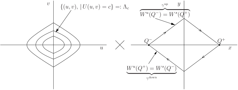
Figure 1: Invariant objects for the unperturbed coupled system.

Even if the periodic orbits $\Lambda_{c}\times Q^{\pm}$ are only continuous manifolds, as $Q^{\pm}$ are hyperbolic critical points, they can be considered hyperbolic periodic orbits. Moreover, their stable and unstable (non-regular) manifolds, $W^{s,u}(\Lambda_{c}\times Q^{\pm})$, are given by $\Lambda_{c}\times W^{s,u}(Q^{\pm})$. Furthermore, the stable/unstable manifold of each periodic orbit $\Lambda_{c}\times Q^{+}$ coincides with the unstable/stable manifold of the periodic orbit $\Lambda_{c}\times Q^{-}$, respectively, and hence there exist (non-regular) heteroclinic manifolds connecting these periodic orbits.
Also of interest are the manifolds $\Lambda^{\pm}$ given by the cross product of the critical points $Q^{\pm}$ with the union of all periodic orbits

$$\Lambda^{+} =\bigcup_{c\in[c_{1},c_{2}]}\Lambda_{c}\times Q^{+}$$

$$=\left\{\left(u,v,Q^{+}\right)\,|\,U(u,v)=c,\,c_{1}\leq c\leq c_{2},\,\right\}$$

$$\Lambda^{-} =\bigcup_{c\in[c_{1},c_{2}]}\Lambda_{c}\times Q^{-}$$

$$=\left\{\left(u,v,Q^{-}\right)\,|\,U(u,v)=c,\,c_{1}\leq c\leq c_{2}\right\},$$

for some $0<c_{1},\,c_{2}<\bar{c}$. In figure 2 we show these two manifolds schematically.

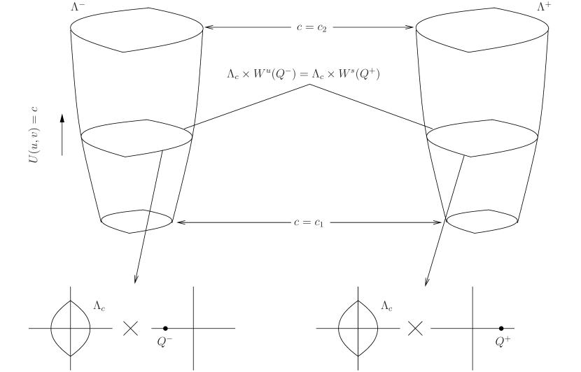
Figure 2: Schematic representation of the manifolds $\Lambda^{+}$ and $\Lambda^{-}$.

2.2 The coupled system

We now consider the system given by coupling systems (2.3) and (2.4) through a non-autonomous $T$-periodic Hamiltonian perturbation $\varepsilon h(u,v,x,y,s)\in C^{\infty}(\mathbb{R}^{5})$ satisfying

$$h(u,v,x,y,s)=h(u,v,x,y,s+T),\;\forall(u,v,x,y,s)\in\mathbb{R}^{5}.$$

Therefore, the perturbed system is a non-autonomous $T$-periodic in time Hamiltonian system with Hamiltonian:

$$H_{\varepsilon}(\tilde{z}):=U(u,v)+X(x,y)+\varepsilon h(\tilde{z}),\;\varepsilon>0,$$ (2.13)

where $\tilde{z}=(z,s)=(u,v,x,y,s)$, $s\in\mathbb{T}_{T}$ and $\mathbb{T}_{T}=\mathbb{R}\backslash T$. To study the dynamics of the corresponding Hamiltonian system we will work in the extended state space $\mathbb{R}^{4}\times\mathbb{T}_{T}$, adding the time $s$ as a state variable. Note that we retain $\mathbb{T}_{T}$, rather than the usual circle (modulus $1$), because $T$ is very important in applications.
Recalling that the unperturbed systems (2.3) and (2.4) are piecewise-smooth, the coupled system is defined in four partitions of $\mathbb{R}^{4}\times\mathbb{T}_{T}$ as follows

$$\left(\begin{array}[]{c}\dot{u}\\ \dot{v}\\ \dot{x}\\ \dot{y}\end{array}\right) =\left\{\begin{aligned} &J_{4}\nabla\left(U^{+}+X^{+}+\varepsilon h\right)\left(\tilde{z}\right)\\ &\hskip 130.08731pt\text{if }\tilde{z}\in S^{+}\cup\Sigma^{+}\times S^{+}\cup\Sigma^{+}\times\mathbb{T}_{T}\\ &J_{4}\nabla\left(U^{+}+X^{-}+\varepsilon h\right)\left(\tilde{z}\right)\\ &\hskip 130.08731pt\text{if }\tilde{z}\in S^{+}\cup\Sigma^{+}\times S^{-}\cup\Sigma^{-}\times\mathbb{T}_{T}\\ &J_{4}\nabla\left(U^{-}+X^{-}+\varepsilon h\right)\left(\tilde{z}\right)\\ &\hskip 130.08731pt\text{if }\tilde{z}\in S^{-}\cup\Sigma^{-}\times S^{-}\cup\Sigma^{-}\times\mathbb{T}_{T}\\ &J_{4}\nabla\left(U^{-}+X^{+}+\varepsilon h\right)\left(\tilde{z}\right)\\ &\hskip 130.08731pt\text{if }\tilde{z}\in S^{-}\cup\Sigma^{-}\times S^{+}\cup\Sigma^{+}\times\mathbb{T}_{T}\end{aligned}\right.$$ (2.14)

$$\dot{s} =1,$$

where $\tilde{z}=(z,s)=(u,v,x,y,s)$, $s\in\mathbb{T}_{T}$ and

$$J_{4}=\left(\begin{array}[]{cccc}0&1&0&0\\ -1&0&0&0\\ 0&0&0&1\\ 0&0&-1&0\end{array}\right).$$

These differential equations define four different autonomous flows $\tilde{\phi}^{\pm\pm}(t;\tilde{z}_{0};\varepsilon)$ in the extended phase space. Letting $\varphi^{\pm\pm}(t;t_{0},z_{0};\varepsilon)$ denote the corresponding non-autonomous flows such that $\varphi^{\pm\pm}(t_{0};t_{0},z_{0};\varepsilon)=z_{0}$, we write $\tilde{\phi}^{\pm\pm}(t;\tilde{z}_{0};\varepsilon)$ satisfying $\tilde{\phi}^{\pm\pm}(0;\tilde{z}_{0};\varepsilon)=\tilde{z}_{0}$ as

$$\tilde{\phi}^{\pm\pm}(t;\tilde{z}_{0};\varepsilon)=\left(\phi^{\pm\pm}(t;\tilde{z}_{0};\varepsilon),s_{0}+t\right),$$

where $\phi^{\pm\pm}(t;\tilde{z}_{0};\varepsilon)$ are such that

$$\varphi^{\pm\pm}(t;t_{0},z_{0};\varepsilon)=\phi^{\pm\pm}(t-t_{0};\tilde{z}_{0};\varepsilon).$$

Proceeding as we did for the systems $\mathcal{U}$ and $\mathcal{X}$, we can define the solution, $\tilde{\phi}(t;\tilde{z}_{0};\varepsilon)$, of the coupled system (2.14) satisfying $\tilde{\phi}(0;\tilde{z}_{0};\varepsilon)=\tilde{z}_{0}$ by properly concatenating the flows $\tilde{\phi}^{+\pm}$ and $\tilde{\phi}^{-\pm}$ when the $4$-dimensional switching manifold $u=0$ is crossed, and $\tilde{\phi}^{\pm+}$ and $\tilde{\phi}^{\pm-}$ when $x=0$ is crossed. Following this definition, we will omit from now on the indices $\pm$ and write just $\tilde{\phi}$. Note that $\tilde{\phi}$ is not differentiable at those times corresponding to the crossings with the switching manifolds, although it is as smooth as the flows $\tilde{\phi}^{\pm\pm}$ when restricted to the open domains given in the respective branches.

Note that, for $\varepsilon=0$, all the invariant objects described in §2.1 for the cross product of the systems (2.3) and (2.4) become invariant objects of system (2.14) with one dimension more in the extended phase space. The study of these objects and their persistence after adding the perturbation will be the goal of section §4.

3 Some notation and properties

3.1 Impact map associated with $u=0$

In $\mathbb{R}^{4}\times\mathbb{T}_{T}$ let us define the sections

$$\tilde{\Sigma}=\Sigma\times\mathbb{R}^{2}\times\mathbb{T}_{T}=\left\{(0,v,x,y,s),\,(v,x,y,s)\in\mathbb{R}^{3}\times\mathbb{T}_{T}\right\}$$ (3.1)

and

$$\tilde{\Sigma}^{+}=\Sigma^{+}\times\mathbb{R}^{2}\times\mathbb{T}_{T}=\left\{(0,v,x,y,s)\in\tilde{\Sigma}\,|\,v>0\right\}$$ (3.2)

$$\tilde{\Sigma}^{-}=\Sigma^{-}\times\mathbb{R}^{2}\times\mathbb{T}_{T}=\left\{(0,v,x,y,s)\in\tilde{\Sigma}\,|\,v<0\right\}.$$ (3.3)

Note that $\tilde{\Sigma}$ is a switching manifold of system (2.14) in the extended phase space, and it will play an important role in what follows.

We wish to define the impact map $P_{\varepsilon}$ associated with $\tilde{\Sigma}$, that is, the Poincaré map from $\tilde{\Sigma}$ to itself (see figure 3). This map is as regular as the flows $\tilde{\phi}^{\pm\pm}$ restricted to some open domains, and this will allow us to apply classical results from perturbation theory of smooth systems that will be useful in our construction.

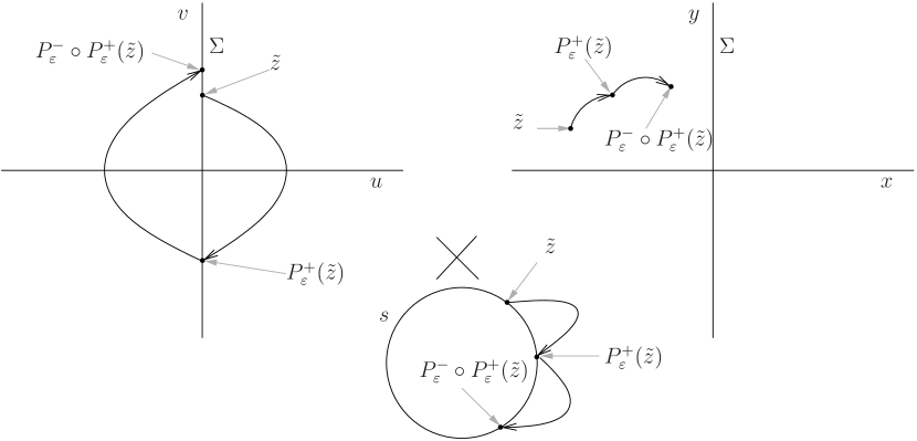
Figure 3: Schematic representation of the maps $P_{\varepsilon}^{-}$, $P_{\varepsilon}^{+}$.

The impact map $P_{\varepsilon}$ is given by the composition of two intermediate maps,

$$P^{+}_{\varepsilon} :\tilde{\mathcal{O}}_{P_{\varepsilon}^{+}}\subset\tilde{\Sigma}^{+}\longrightarrow\tilde{\Sigma}^{-}$$ (3.4)

$$P^{-}_{\varepsilon} :\tilde{\mathcal{O}}_{P_{\varepsilon}^{-}}\subset\tilde{\Sigma}^{-}\longrightarrow\tilde{\Sigma}^{+}$$ (3.5)

defined as

$$P_{\varepsilon}^{+}(\tilde{z}) =\tilde{\phi}(t_{\tilde{\Sigma}^{-}};\tilde{z};\varepsilon)$$

$$P_{\varepsilon}^{-}(\tilde{z}) =\tilde{\phi}(t_{\tilde{\Sigma}^{+}};\tilde{z};\varepsilon),$$

where $t_{\tilde{\Sigma}^{\pm}}$ are the smallest values of $t>0$ such that $\tilde{\phi}(t;\tilde{z};\varepsilon)\in\tilde{\Sigma}^{\mp}$. The domains $\tilde{\mathcal{O}}_{P_{\varepsilon}^{\pm}}$ where these maps are smooth are the open sets given by points in $\tilde{\Sigma}^{\pm}$ whose trajectories first impact the switching manifold $\tilde{\Sigma}$ given by $u=0$ rather than the switching manifold $x=0$. That is,

$$\tilde{\mathcal{O}}_{P_{\varepsilon}^{+}}=\left\{\tilde{z}\in\tilde{\Sigma}^{+},|\,\Pi_{x}\left(\tilde{\phi}(t;\tilde{z};\varepsilon)\right)\neq 0\,\forall t\in[0,t_{\tilde{\Sigma}^{-}}]\right\}$$ (3.6)

and

$$\tilde{\mathcal{O}}_{P_{\varepsilon}^{-}}=\left\{\tilde{z}\in\tilde{\Sigma}^{-},|\,\Pi_{x}\left(\tilde{\phi}(t;\tilde{z};\varepsilon)\right)\neq 0\,\forall t\in[0,t_{\tilde{\Sigma}^{+}}]\right\}.$$

Remark 3.1.

Due to the form of the Hamiltonian $X$ given in (2.5), for $\varepsilon\geq 0$ small enough the flow crosses the switching manifold $x=0$ for increasing $x$ when $y>0$ and for decreasing $x$ for $y<0$. Hence, the points in $\tilde{\mathcal{O}}_{P_{\varepsilon}^{+}}$ and $\tilde{\mathcal{O}}_{P_{\varepsilon}^{-}}$ can be arbitrarily close to $x=0$ when $xy\geq 0$ (possibly containing some part of the segment $x=0$) but not when $xy<0$. This implies that the sets $\tilde{\mathcal{O}}_{P_{\varepsilon}^{\pm}}$ consist of two connected components separated by the switching manifold $x=0$, $\mathbb{R}^{2}\times\Sigma\times\mathbb{T}_{T}$. How these sets are separated from $x=0$ depends on the time required to reach the switching manifold $u=0$.

Let us consider an open set,

$$\tilde{\mathcal{O}}_{P_{\varepsilon}}\subset\tilde{\mathcal{O}}_{P_{\varepsilon}^{+}}\cup\tilde{\mathcal{O}}_{P_{\varepsilon}^{-}}\subset\tilde{\Sigma},$$ (3.7)

and define the Poincaré impact map

$$P_{\varepsilon}:\tilde{\mathcal{O}}_{P_{\varepsilon}}\subset\tilde{\Sigma}\longrightarrow\tilde{\Sigma}$$

as

$$P_{\varepsilon}(0,v,x,y,s)=\left\{\begin{aligned} &P_{\varepsilon}^{+}\circ P_{\varepsilon}^{-}(0,v,x,y,s)&&\text{if }\left(0,v,x,y,s\right)\in\tilde{\mathcal{O}}_{P_{\varepsilon}}\cap\tilde{\Sigma}^{-}\\ &P_{\varepsilon}^{-}\circ P_{\varepsilon}^{+}(0,v,x,y,s)&&\text{if }\left(0,v,x,y,s\right)\in\tilde{\mathcal{O}}_{P_{\varepsilon}}\cap\tilde{\Sigma}^{+}\end{aligned}\right.$$

To simplify notation, when considering points $(0,v,x,y,s)\in\tilde{\Sigma}\subset\mathbb{R}^{4}\times\mathbb{T}_{T}$, we introduce the new variable $\tilde{\omega}=(v,x,y,s)$. Then points $\tilde{z}$ in $\mathbb{R}^{4}\times\mathbb{T}_{T}$ will be written as $\tilde{z}=(0,\tilde{\omega})$. In addition we consider the set $\tilde{\mathcal{O}}_{P_{\varepsilon}}$ in $\mathbb{R}^{3}\times\mathbb{T}_{T}$ and write the impact map

$$P_{\varepsilon}:\tilde{\mathcal{O}}_{P_{\varepsilon}}\longrightarrow\mathbb{R}^{3}\times\mathbb{T}_{T}$$ (3.8)

as

$$P_{\varepsilon}(\tilde{\omega})=\left\{\begin{aligned} &P_{\varepsilon}^{+}\circ P_{\varepsilon}^{-}(\tilde{\omega})&&\text{if }\tilde{\omega}\in\tilde{\mathcal{O}}_{P_{\varepsilon}}\cap\left\{(v,x,y,s)\in\mathbb{R}^{3}\times\mathbb{T}_{T},\,v<0\right\}\\ &P_{\varepsilon}^{-}\circ P_{\varepsilon}^{+}(\tilde{\omega})&&\text{if }\tilde{\omega}\in\tilde{\mathcal{O}}_{P_{\varepsilon}}\cap\left\{(v,x,y,s)\in\mathbb{R}^{3}\times\mathbb{T}_{T},\,v>0\right\}\end{aligned}\right.$$ (3.9)

with

$$\tilde{\mathcal{O}}_{P_{\varepsilon}}=\Big{\{} \tilde{\omega}=(v,x,y,s)\in\left([-v_{2},-v_{1}]\cup[v_{1},v_{2}]\right)\times\mathbb{R}^{2}\times\mathbb{T}_{T}$$

$$|\,\Pi_{x}\left(\tilde{\phi}(t;\left(0,\tilde{\omega}\right);\varepsilon)\right)\neq 0\,\forall t\in\left[0,\Pi_{s}\left(P_{\varepsilon}(\tilde{\omega})\right)-s\right]\Big{\}}.$$

Note that the map $P_{\varepsilon}$ is invertible in $\tilde{\mathcal{O}}_{P_{\varepsilon}^{-1}}:=P_{\varepsilon}(\tilde{\mathcal{O}}_{P_{\varepsilon}})$ and hence we can consider

$$P_{\varepsilon}^{-1}:\tilde{\mathcal{O}}_{P_{\varepsilon}^{-1}}\subset\mathbb{R}^{3}\times\mathbb{T}_{T}\longrightarrow\mathbb{R}^{3}\times\mathbb{T}_{T}.$$ (3.10)

Remark 3.2.

Although the maps $P^{+}_{\varepsilon}$, $P^{-}_{\varepsilon}$, $P_{\varepsilon}$ can be defined in a wider zone of the extended phase space, their restriction to the domains $\tilde{\mathcal{O}}_{P_{\varepsilon}^{+}}$, $\tilde{\mathcal{O}}_{P_{\varepsilon}^{-}}$, $\tilde{\mathcal{O}}_{P_{\varepsilon}}$ will be essential in our contructions. The reason is that the maps $P^{+}_{\varepsilon}$, $P^{-}_{\varepsilon}$, $P_{\varepsilon}$ are, in the domains $\tilde{\mathcal{O}}_{P_{\varepsilon}^{+}}$, $\tilde{\mathcal{O}}_{P_{\varepsilon}^{-}}$, $\tilde{\mathcal{O}}_{P_{\varepsilon}}$ respectively, as smooth as the flows $\tilde{\phi}^{\pm\pm}(t;\tilde{z};\varepsilon)$ restricted to $S^{\pm}\times S^{\pm}\times\mathbb{T}_{T}$. Therefore, we can apply to them classical results of smooth dynamical systems which need regularity assumptions.

If $\varepsilon=0$, we can provide an explicit expression for the impact map as follows. The flow $\tilde{\phi}(t;\tilde{z}_{0};0)$ consists of the uncoupled flows $\phi_{\mathcal{U}}$ and $\phi_{\mathcal{X}}$ described in (2.8) but extended by adding the time $s$ as a state variable. From conditions C.1–C.4, the phase portrait of system $\mathcal{U}$ is formed by the continuum of periodic orbits $\Lambda_{c}$ which, due to the form of the Hamiltonian $U$, is symmetric with respect to $v=0$. Hence the maps $P_{0}^{\pm}$ can be written as

$$P_{0}^{\pm}(\tilde{z})=\left(0,-v,\phi_{\mathcal{X}}(\alpha^{\pm}(v);x,y),s+\alpha^{\pm}(v)\right),$$

where

$$\alpha^{\pm}(v)=2\mspace{-30.0mu}\mathop{\int}_{0}^{(V^{\pm})^{-1}(c)}\mspace{-30.0mu}\frac{1}{\sqrt{2(c-V^{\pm}(x))}}dx,\quad c=U(0,v)=\frac{v^{2}}{2}$$ (3.11)

are the times taken by the flow $\phi_{\mathcal{U}}(t;0,\pm v)$, with $v>0$, to reach $\Sigma^{\mp}$. Hence, when $\varepsilon=0$, the impact map takes the form

$$P_{0}(\tilde{\omega})=\left(v,\phi_{\mathcal{X}}(\alpha(v);x,y),s+\alpha(v)\right),$$

where

$$\alpha(v)=\alpha^{+}(|v|)+\alpha^{-}(-|v|)$$ (3.12)

is the period of the orbit of system (2.4) with $c=U(0,v)$, and $\phi_{\mathcal{X}}(t;x,y)=\phi^{\pm}_{\mathcal{X}}(t;x,y)$ if $(x,y)\in\Sigma^{\pm}\cup S^{\pm}$.

3.2 Impact sequence

Let $\tilde{\omega}\in\tilde{\mathcal{O}}_{P_{\varepsilon}}$ and $\varepsilon\geq 0$ small enough. Proceeding as in [Hog89, GHS12], we define the direct sequence of impacts $\tilde{\omega}_{i}$ associated with the section $\tilde{\Sigma}$ as

$$\tilde{\omega}_{i}=\left\{\begin{aligned} &P^{+}_{\varepsilon}(\tilde{\omega}_{i-1})&&\text{if }\tilde{\omega}_{i-1}\in\tilde{\mathcal{O}}_{P_{\varepsilon}^{+}}\\ &P^{-}_{\varepsilon}(\tilde{\omega}_{i-1})&&\text{if }\tilde{\omega}_{i-1}\in\tilde{\mathcal{O}}_{P_{\varepsilon}^{-}},\end{aligned}\right.$$ (3.13)

with $i\geq 0$ and $\tilde{\omega}_{0}=\tilde{\omega}$. We also define the inverse sequence of impacts, if they exist, as

$$\tilde{\omega}_{i}=\left\{\begin{aligned} &(P^{+}_{\varepsilon})^{-1}(\tilde{\omega}_{i+1})&&\text{if }\tilde{\omega}_{i+1}\in P^{+}_{\varepsilon}(\tilde{\mathcal{O}}_{P_{\varepsilon}^{+}})\\ &(P^{-}_{\varepsilon})^{-1}(\tilde{\omega}_{i+1})&&\text{if }\tilde{\omega}_{i+1}\in P^{-}_{\varepsilon}(\tilde{\mathcal{O}}_{P_{\varepsilon}^{-}}),\end{aligned}\right.$$ (3.14)

with $i<0$. In general, this is a finite sequence, and is defined up to the $n$th iterate such that

$$\tilde{\omega}_{n}\notin\tilde{\mathcal{O}}_{P_{\varepsilon}^{+}}\cup\tilde{\mathcal{O}}_{P_{\varepsilon}^{-}},\,n>0$$

$$\tilde{\omega}_{n}\notin P_{\varepsilon}^{-}\left(\tilde{\mathcal{O}}_{P_{\varepsilon}^{-}}\right)\cup P_{\varepsilon}^{+}\left(\tilde{\mathcal{O}}_{P_{\varepsilon}^{+}}\right),\,n<0$$

That is, we consider all the impacts with the switching surface $u=0$ of the trajectory associated with system (2.14) with initial condition $\tilde{z}$ that are previous to the first impact with $x=0$, both forwards and backwards in time. When this occurs, then it is possible to extend the sequence by properly concatenating the flow.

In general, one can extend the definition of the impact sequence to arbitrary points in $\tilde{z}\in S^{\pm}\times S^{\pm}\times\mathbb{T}_{T}$, no necessarily located at $\tilde{\Sigma}$. This can be done by flowing $\tilde{z}$ by $\tilde{\phi}$ both forwards and backwards in time until the switching manifold $\tilde{\Sigma}$ is reached at the points $\tilde{z}_{1}\in\tilde{\mathcal{O}}_{P_{\varepsilon}}$ and $\tilde{z}_{2}\in\tilde{\mathcal{O}}_{P_{\varepsilon}}$, respectively. Then, one just considers the direct and inverse impact sequence of associated with the points $\tilde{z}_{1}$ and $\tilde{z}_{2}$, respectively.

Note that the impact sequence can be used to obtain explicit expressions for the flows (see [Gra12] for details).

4 Invariant manifolds and their persistence

4.1 Unperturbed case in the extended phase space

We consider invariant objects of system (2.14) when $\varepsilon=0$. The cross products of the hyperbolic critical points $Q^{\pm}$ and the periodic orbits $\Lambda_{c}$ give rise to two families of invariant $2$-dimensional tori $\tilde{\mathcal{T}}_{c}^{\pm}$ of the form

$$\tilde{\mathcal{T}}_{c}^{\pm} =\Lambda_{c}\times Q^{\pm}\times\mathbb{T}_{T}=$$

$$\left\{(u,v,x,y,s)\,|\,U(u,v)=c,\,(x,y)=Q^{\pm}\!,s\in\mathbb{T}_{T}\right\}$$ (4.1)

with $0<c\leq\bar{c}$. These tori are only continuous manifolds, because of the singularity of the Hamiltonian $U$ at $u=0$ (see figure 4).

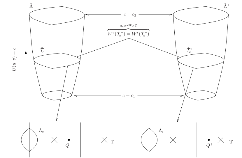
Figure 4: Scheme of the manifolds $\tilde{\Lambda}^{\pm}$, the tori $\tilde{\mathcal{T}}_{c}^{\pm}$ and their invariant manifolds.

We parameterize $\tilde{\mathcal{T}}_{c}^{\pm}$ by

$$\tilde{\mathcal{T}}_{c}^{\pm}=\left\{(\phi_{\mathcal{U}}(\theta\alpha(v);0,v),Q^{\pm},s),\,\theta\in\mathbb{T},\,v\in\mathbb{R},\,U(0,v)=c,\,s\in\mathbb{T}_{T}\right\},$$ (4.2)

where $\alpha(v)$ is given in (3.12), $\mathbb{T}=\mathbb{R}\backslash\mathbb{Z}$ is the usual circle and $\phi_{\mathcal{U}}$ is the flow associated with system (2.4). Then the flow $\tilde{\phi}$ restricted to these tori becomes

$$\tilde{\phi}(t; \phi_{\mathcal{U}}(\theta\alpha(v);0,v),Q^{\pm},s;0)$$

$$=\left(\phi_{\mathcal{U}}\left(\left(\theta+\frac{t}{\alpha(v)}\right)\alpha(v);0,v\right),Q^{\pm},s+t\right),\,\forall t\in\mathbb{R},$$

and hence $\tilde{\mathcal{T}}_{c}^{\pm}$ is invariant. For each of these invariant tori there exist $3$-dimensional continuous manifolds

$$W^{s} (\tilde{\mathcal{T}}_{c}^{+})=W^{u}(\tilde{\mathcal{T}}_{c}^{-})$$

$$=\Lambda_{c}\times W^{s}(Q^{-})\times\mathbb{T}_{T}=\Lambda_{c}\times W^{u}(Q^{+})\times\mathbb{T}_{T}$$

$$=\left\{(\phi_{\mathcal{U}}(\theta\alpha(v);0,v),\sigma^{\text{up}}(\xi),s),|\,U(0,v)=c,\,\theta\in\mathbb{T},\,\xi\in\mathbb{R},\,s\in\mathbb{T}_{T}\right\},$$

where $\sigma^{\text{up}}(\xi)$, given in (2.10)-(2.11), parameterizes the upper heteroclinic connection $\gamma^{\text{up}}$ of system $\mathcal{X}$ (see figure 4). The flow $\tilde{\phi}$ restricted to these manifolds can be written as

$$\tilde{\phi}(t; \phi_{\mathcal{U}}(\theta\alpha(v);0,v),\sigma^{\text{up}}(\xi),s;0)$$

$$=\left(\phi_{\mathcal{U}}\left(\left(\theta+\frac{t}{\alpha(v)}\right)\alpha(v);0,v\right),\sigma^{\text{up}}(\xi+t),s+t\right),\,\forall t\in\mathbb{R},$$

and hence they are invariant. Moreover, for any $\tilde{z}=\left(\phi_{\mathcal{U}}(\theta\alpha(v);0,v),\sigma^{\text{up}}(\xi),s\right)\in W^{s}(\tilde{\mathcal{T}}_{c}^{+})=W^{u}(\tilde{\mathcal{T}}_{c}^{-})$, there exists two points

$$\tilde{z}^{\pm}=\left(\phi_{\mathcal{U}}(\theta\alpha(v);0,v),Q^{\pm},s\right)\in\tilde{\mathcal{T}}_{c}^{\pm}$$

such that

$$\lim_{t\to\pm\infty}\left|\tilde{\phi}(t;\tilde{z};0)-\tilde{\phi}(t;\tilde{z}^{\pm};0)\right|=\lim_{t\to\pm\infty}\left(0,0,\sigma^{\text{up}}(\xi+t)-Q^{\pm},0\right)=0.$$

In addition, as the points $Q^{\pm}$ are hyperbolic for the flows $\phi^{\pm}_{\mathcal{X}}$, then there exist positive constants $K^{\pm}$ such that

$$\left|\phi(t;\tilde{z};0)-\phi(t;\tilde{z}^{\pm};0)\right|<K^{\pm}e^{-\lambda^{\pm}|t|},\,t\to\pm\infty,$$ (4.3)

where $\pm\lambda^{+}$ and $\pm\lambda^{-}$ are the eigenvalues of $D\mathcal{X}^{+}(Q^{+})$ and $D\mathcal{X}^{-}(Q^{-})$, respectively.
Although $W^{u,s}(\tilde{\mathcal{T}}_{c}^{\pm})$ are just continuous manifolds, they are the stable and unstable manifolds of $\tilde{\mathcal{T}}_{c}^{\pm}$. As they coincide, $\tilde{\gamma}^{\text{up}}_{c}:=W^{s}(\tilde{\mathcal{T}}_{c}^{+})=W^{u}(\tilde{\mathcal{T}}_{c}^{-})$ will be a $3$-dimensional heteroclinic manifold between the tori $\tilde{\mathcal{T}}_{c}^{-}$ and $\tilde{\mathcal{T}}_{c}^{+}$. The lower heteroclinic connection mentioned in condition C.2 leads to similar heteroclinic manifolds between the tori $\tilde{\mathcal{T}}_{c}^{+}$ and $\tilde{\mathcal{T}}_{c}^{-}$.

Following [DdlLS00], considering all the tori $\tilde{\mathcal{T}}^{+}_{c}$ and $\tilde{\mathcal{T}}^{-}_{c}$ together we end up with two $3$-dimensional continuous manifolds

$$\tilde{\Lambda}^{\pm} =\bigcup_{c\in[c_{1},c_{2}]}\tilde{\mathcal{T}}_{c}^{\pm}=\bigcup_{c\in[c_{1},c_{2}]}\Lambda_{c}\times Q^{\pm}\times\mathbb{T}_{T}$$

$$=\left\{\left(u,v,x,y,s\right),\,c_{1}\leq U(u,v)\leq c_{2},\,(x,y)=Q^{\pm},\,s\in\mathbb{T}_{T}\right\}$$

$$=\left\{\left(\phi_{\mathcal{U}}(\theta\alpha(v);0,v),Q^{\pm},s\right),\,\theta\in\mathbb{T},\,c_{1}\leq U(0,v)\leq c_{2},\,s\in\mathbb{T}_{T}\right\}$$ (4.4)

with $0<c_{1}<c_{2}<\bar{c}$, shown schematically in figure 4. These manifolds have $4$-dimensional stable and unstable continuous manifolds given by

$$W^{s} (\tilde{\Lambda}^{+})=W^{u}(\tilde{\Lambda}^{-})=\bigcup_{c\in[c_{1},c_{2}]}W^{s}(\tilde{\mathcal{T}}^{+}_{c})=\bigcup_{c\in[c_{1},c_{2}]}W^{u}(\tilde{\mathcal{T}}^{-}_{c})$$

$$=\left\{\left(\phi_{\mathcal{U}}(\theta\alpha(v);0,v),\sigma^{\text{up}}(\xi),s\right),\,\theta\in\mathbb{T},\,c_{1}\leq U(0,v)\leq c_{2},\,\xi\in\mathbb{R},\,s\in\mathbb{T}_{T}\right\}.$$ (4.5)

As they coincide, $\tilde{\gamma}^{\text{up}}:=W^{s}(\tilde{\Lambda}^{+})=W^{u}(\tilde{\Lambda}^{-})$ will be a $4$-dimensional heteroclinic continuous manifold between the manifolds $\tilde{\Lambda}^{\pm}$.

It will be convenient to write the manifolds $\tilde{\Lambda}^{\pm}$ in terms of a reference manifold $N$ (see [DdlLS08]) as follows. Let

$$N=\left\{(\theta,v,s)\in\mathbb{T}\times[v_{1},v_{2}]\times\mathbb{T}_{T}\right\}$$ (4.6)

where $c_{i}=U(0,v_{i})$, and consider two homeomorphisms

$$\begin{array}[]{cccc}F_{0}^{\pm}:&N&\longrightarrow&\tilde{\Lambda}^{\pm}\\ &(\theta,v,s)&\longmapsto&(\phi_{\mathcal{U}}(\theta\alpha(v);0,v),Q^{\pm},s).\end{array}$$ (4.7)

Hence the continuous manifolds $\tilde{\Lambda}^{\pm}$ are given by $\tilde{\Lambda}^{\pm}=F_{0}^{\pm}(N)$. This will later allow us to identify points on the perturbed manifolds $\tilde{\Lambda}_{\varepsilon}^{\pm}$ in terms of the same coordinates $(\theta,v,s)$ if $\varepsilon>0$ is small enough. Note that $F_{0}^{\pm}$ are in fact diffeomorphisms as long as $\theta\in\left(0,\frac{\alpha^{+}(v)}{\alpha(v)}\right)\cup\left(\frac{\alpha^{+}(v)}{\alpha(v)},1\right)$ as $\phi_{\mathcal{U}}(\theta\alpha(v);0,v)$ hits the switching manifold given by $u=0$ for $\theta=0$, $\theta=\frac{\alpha^{+}(v)}{\alpha(v)}$ and $\theta=1$.

4.2 Invariant manifolds for the unperturbed impact map

The fact that the manifolds $\tilde{\Lambda}^{\pm}$ are only continuous manifolds will prevent us from applying classical perturbation theory for hyperbolic manifolds [Fen72, Fen74, Fen77, HPS77, DdlLS00] to study their persistence for $\varepsilon>0$. In the smooth case, the usual tool to prove persistence following a non-autonomous periodic perturbation is the stroboscopic Poincaré map, which integrates the system during a certain time $T$, the period of the perturbation. However, in our case, such a map becomes unwieldy because, for a given time, the number of occasions that the switching manifold can be crossed is unknown and can even be arbitrarily large.

Instead, we will consider the Poincaré impact map defined in §3.1, which is a smooth map as regular as the flows $\tilde{\phi}^{\pm\pm}$ restricted to their respective domains. We first describe the invariant objects introduced above for the impact map restricted to $\tilde{\Sigma}^{+}$ when $\varepsilon=0$. As mentioned in §3.1, we will identify the switching manifold $\tilde{\Sigma}^{+}$ with the set $[v_{1},v_{2}]\times\mathbb{R}^{2}\times\mathbb{T}_{T}$ and omit the repetition of the coordinate $u=0$ for points in $\tilde{\Sigma}$. We then consider the unperturbed impact map

$$P_{0}:\tilde{\mathcal{O}}_{P_{0}}\cap\left\{(v,x,y,s)\in\mathbb{R}^{3}\times\mathbb{T}_{T},\,v>0\right\}\longrightarrow\mathbb{R}^{3}\times\mathbb{T}_{T}.$$

Taking into account that

$$P_{0}(v,Q^{\pm},s)=(v,Q^{\pm},s+\alpha(v)),$$ (4.8)

and letting $U\left(0,v\right)=c$, the invariant tori $\tilde{\mathcal{T}}_{c}^{\pm}$ give rise to smooth invariant curves

$$\tilde{\mathcal{C}}_{c}^{\pm} =\left\{v\right\}\times Q^{\pm}\times\mathbb{T}_{T}$$

$$=\left\{(v,x,y,s)\in\mathbb{R}^{3}\times\mathbb{T}_{T},\,U(0,v)=c,\,(x,y)=Q^{\pm}\right\}$$ (4.9)

with $0<c\leq\bar{c}$. For those values of $c$ such that $m\alpha(v)=nT$, for some natural numbers $n$ and $m$, the curves $\tilde{\mathcal{C}}_{c}^{\pm}$ are filled by periodic points. The rest are formed by points whose trajectories are dense in $\tilde{\mathcal{C}}_{c}^{\pm}$.

For each of these curves there exist $2$-dimensional (locally smooth) continuous manifolds

$$W^{s}(\tilde{\mathcal{C}}_{c}^{+}) =W^{u}(\tilde{\mathcal{C}}_{c}^{-})$$

$$=\left\{\left(v,\sigma^{\text{up}}(\xi),s\right),\,U(0,v)=c,\,\xi\in\mathbb{R},\,s\in\mathbb{T}_{T}\right\}$$

which are invariant under $P_{0}$:

$$P_{0}(v,\sigma^{\text{up}}(\xi),s)=\left(v,\sigma^{\text{up}}(\xi+\alpha(v)),s+\alpha(v))\right)\in W^{u}(\tilde{\mathcal{C}}_{c}^{-})=W^{s}(\tilde{\mathcal{C}}_{c}^{+}).$$

Moreover, due to the hyperbolicity of the points $Q^{\pm}$ (see (4.3)), for any $\tilde{\omega}=(v,\sigma^{\text{up}}(\xi),s)\in W^{u}(\tilde{\mathcal{C}}_{c}^{-})=W^{s}(\tilde{\mathcal{C}}_{c}^{+})$, there exist $\tilde{\omega}^{\pm}=(v,Q^{\pm},s)\in\tilde{\mathcal{C}}_{c}^{\pm}$ such that

$$|P^{n}_{0}(\tilde{\omega})-P_{0}^{n}(\tilde{\omega}^{\pm})|=\left|\left(0,\sigma^{\text{up}}\left(\xi+n\alpha\left(v\right)\right)-Q^{\pm},0\right)\right|<\hat{K}^{\pm}(\hat{\lambda}^{\pm})^{|n|},\,n\to\pm\infty,$$ (4.10)

where $\hat{K}^{\pm}=K^{\pm}e^{-\lambda^{\pm}\xi}$, $0<\hat{\lambda}^{\pm}=e^{-\lambda^{\pm}\alpha(v)}<1$ and $\lambda^{\pm},K^{\pm}$ are defined in (4.3).

Proceeding similarly as with the flow, we now consider the union over $c$ of all the curves $\tilde{\mathcal{C}}^{\pm}_{c}$ which become the smooth cylinders

$$\tilde{\Gamma}^{\pm}=\bigcup_{c\in[c_{1},c_{2}]}\tilde{\mathcal{C}}_{c}^{\pm}=\left\{(v,Q^{\pm},s)\,|\,v_{1}<v<v_{2},\,s\in\mathbb{T}_{T}\right\}\\$$ (4.11)

with $0<c_{i}\leq\bar{c}$ and $c_{i}=U(0,v_{i})$, $i=1,2$, which are invariant under $P_{0}$. Note that the manifolds $\tilde{\Gamma}^{\pm}$ correspond to the intersection

$$\tilde{\Lambda}^{\pm}\cap\tilde{\Sigma}^{+}=\left\{0\right\}\times\tilde{\Gamma}^{\pm}.$$

Taking into account that $\tilde{\Gamma}^{\pm}$ are compact manifolds with boundaries given by $v=v_{1}$ and $v=v_{2}$, there exist constants $\bar{\mu}>1$, $0<\bar{\lambda}^{\pm}<1$, $\bar{\lambda}^{\pm}<\frac{1}{\bar{\mu}}$ (in fact $\bar{\mu}$ can be taken as close to one as desired) such that, for all $\tilde{\omega}\in\tilde{\Gamma}^{\pm}$

$$\begin{array}[]{lcll}w\in E_{\tilde{\omega}}^{s}&\Longleftrightarrow&|DP_{0}^{n}(\tilde{\omega})w|\leq K^{\pm}(\bar{\lambda}^{\pm})^{n}|w|,&\,n\geq 0\\ w\in E_{\tilde{\omega}}^{u}&\Longleftrightarrow&|DP_{0}^{n}(\tilde{\omega})w|\leq K^{\pm}(\bar{\lambda}^{\pm})^{-n}|w|,&\,n\leq 0\\ w\in T_{\tilde{\omega}}\tilde{\Gamma}^{\pm}&\Longleftrightarrow&|DP^{n}_{0}(\tilde{\omega})w|\leq K^{\pm}(\bar{\mu})^{|n|}|w|,&\,n\in\mathbb{Z}\end{array}$$ (4.12)

where $E_{\tilde{\omega}}^{s},E_{\tilde{\omega}}^{u}$ and $T_{\tilde{\omega}}\tilde{\Gamma}^{\pm}$ are the stable, unstable and tangent bundles of $\tilde{\Gamma}^{\pm}$ respectively. Assuming that $\alpha(v)$ is an increasing function of $v$, we can take

$$\bar{\lambda}^{\pm}=e^{-\alpha(v_{1})\lambda^{\pm}}.$$ (4.13)

Hence, $\tilde{\Gamma}^{\pm}$ are $C^{\infty}$ (as regular as the flows) normally hyperbolic manifolds for the unperturbed impact map $P_{0}$, with stable and unstable invariant manifolds

$$W^{u}(\tilde{\Gamma}^{-}) =W^{s}(\tilde{\Gamma}^{+})=\bigcup_{c\in[c_{1},c_{2}]}W^{u}(\tilde{\mathcal{C}}_{c}^{-})=\bigcup_{c\in[c_{1},c_{2}]}W^{s}(\tilde{\mathcal{C}}_{c}^{+})$$

$$=\left\{(v,\sigma^{\text{up}}(\xi),s),\,v_{1}\leq v\leq v_{2},\,\xi\in\mathbb{R},\,s\in\mathbb{T}_{T}\right\}.$$

4.3 Perturbed case

Let us now consider the persistence of the invariant manifolds introduced in the previous section when $\varepsilon>0$ is small. We first focus on the normally hyperbolic manifolds, $\tilde{\Gamma}^{\pm}$, for the map $P_{0}$. As mentioned in Remark 3.2, the impact map $P_{\varepsilon}$ is, in $\tilde{\mathcal{O}}_{P_{\varepsilon}}$, as regular as the flows $\tilde{\phi}^{\pm\pm}$ restricted to $S^{\pm}\times S^{\pm}\times\mathbb{T}_{T}$. Thus, the persistence of the normally hyperbolic manifolds $\tilde{\Gamma}^{\pm}$ for $\varepsilon>0$ comes from the theory of normally hyperbolic manifolds [HP70, Fen72, Fen74, HPS77, DdlLS08]. This guarantees the existence of normally hyperbolic invariant manifolds $\tilde{\Gamma}_{\varepsilon}^{\pm}$ and $\mathcal{C}^{r}$ diffeomorphisms (with $r$ as big as we want)

$$G_{\varepsilon}^{\pm} :\mathbb{R}\times\mathbb{T}_{T}\longrightarrow\mathbb{R}^{3}\times\mathbb{T}_{T},$$

$$g_{\varepsilon}^{\pm} :\mathbb{R}\times\mathbb{T}_{T}\longrightarrow\mathbb{R}^{2}$$

such that the points at the manifolds $\tilde{\Gamma}_{\varepsilon}^{+}$ are parameterized by $\tilde{\omega}^{\pm}=G_{\varepsilon}^{\pm}(v,s)\in\tilde{\Gamma}_{\varepsilon}^{\pm}.$ These parameterizations are not unique. We can make them unique by taking $G_{\varepsilon}^{\pm}$ to be the identity in the $v$ and $s$ coordinates,

$$\Pi_{v,s}\left(G_{\varepsilon}^{\pm}\right)=Id,$$ (4.14)

that is,

$$G_{\varepsilon}^{\pm}(v,s)=(v,g_{\varepsilon}^{\pm}(v,s),s).$$

When $\varepsilon=0$, these maps coincide with the parametrization defined in (4.11). Therefore $g_{0}^{\pm}(v,s)=Q^{\pm}$ and $\tilde{\Gamma}_{\varepsilon}^{+}$ is $\varepsilon$-close to $\tilde{\Gamma}^{+}$. In particular, $\tilde{\Gamma}_{\varepsilon}^{\pm}\subset\tilde{\mathcal{O}}_{\varepsilon}$.

The manifolds $\tilde{\Gamma}_{\varepsilon}^{\pm}$ have $\mathcal{C}^{r}$ local stable and unstable manifolds

$$W^{s,u}(\tilde{\Gamma}_{\varepsilon}^{\pm})$$

$\varepsilon$-close to $W^{s,u}(\tilde{\Gamma}^{\pm})$, satisfying:

• For every $\tilde{\omega}^{s}\in W^{s}(\tilde{\Gamma}_{\varepsilon}^{+})$ there exists $\tilde{\omega}^{+}\in\tilde{\Gamma}_{\varepsilon}^{+}$ such that:

  $$|P^{n}_{\varepsilon}(\tilde{\omega}^{s})-P^{n}_{\varepsilon}(\tilde{\omega}^{+})|<K^{+}\left(\bar{\lambda}^{+}+O(\varepsilon)\right)^{n}\to 0,\,n\to+\infty,$$ (4.15)

• For every $\tilde{\omega}^{u}\in W^{u}(\tilde{\Gamma}_{\varepsilon}^{+})$ there exists $\tilde{\omega}^{+}\in\tilde{\Gamma}_{\varepsilon}^{+}$ such that:

  $$|P^{n}_{\varepsilon}(\tilde{\omega}^{u})-P^{n}_{\varepsilon}(\tilde{\omega}^{+})|<K^{+}\left(\bar{\lambda}^{+}+O(\varepsilon)\right)^{-n}\to 0,\,n\to-\infty,$$ (4.16)

and $0<\bar{\lambda}^{+}<1$ is the constant given in (4.12). Analogous properties hold for the manifold $\tilde{\Gamma}_{\varepsilon}^{-}$.

Remark 4.1.

In general, the theorem of persistence of normally hyperbolic manifolds only gives local invariance for the perturbed manifold. Nevertheless, following [KKY97], one can use the change of variables given in [Lev91] to obtain the impact map in symplectic coordinates. Therefore, one can apply the twist theorem to the perturbed impact map. This gives that those curves $\tilde{\mathcal{C}}_{c}\subset\tilde{\Gamma}_{0}^{\pm}$ with $\alpha(\sqrt{2c})/T$ far away from rational numbers persist as invariant curves. These provide invariant boundaries for the perturbed manifolds $\tilde{\Gamma}_{\varepsilon}^{\pm}$, and hence these are compact invariant manifolds.

We now consider the existence of manifolds equivalent to $\tilde{\Gamma}^{\pm}_{\varepsilon}$ for the flow $\tilde{\phi}$. More precisely, we are interested in obtaining the perturbed version of the manifolds $\tilde{\Lambda}^{\pm}$ in terms of the reference manifold $N$ given in (4.6).

Proposition 4.1.

Let $\tilde{\Lambda}^{\pm}$ and $W^{s,u}(\tilde{\Lambda}^{\pm})$ be the manifolds described in §4.1 invariant for the unperturbed system (2.14). Then, there exist continuous maps

$$F_{\varepsilon}^{\pm}:N\longrightarrow\mathbb{R}^{4}\times\mathbb{T}_{T},$$

where $F_{0}^{\pm}$ are given in (4.7), that are Lipschitz in $\varepsilon$, such that the $C^{0}$ manifolds

$$\tilde{\Lambda}_{\varepsilon}^{\pm}=F_{\varepsilon}^{\pm}(N)$$ (4.17)

are invariant under $\tilde{\phi}$ and $\varepsilon$-close to $\tilde{\Lambda}^{\pm}$. Moreover, there exist $C^{0}$ manifolds $W^{s,u}(\tilde{\Lambda}_{\varepsilon}^{\pm})$, $\varepsilon$-close to $W^{s,u}(\tilde{\Lambda}^{+})$, satisfying:

• for any $\tilde{z}^{s}=(z^{s},s^{s})\in W^{s}(\tilde{\Lambda}_{\varepsilon}^{+})$ there exists $\tilde{z}^{+}=(z^{+},s^{+})\in\tilde{\Lambda}_{\varepsilon}^{+}$ such that

  $$|\tilde{\phi}(t;\tilde{z}^{s};\varepsilon)-\tilde{\phi}(t;\tilde{z}^{+};\varepsilon)|<\bar{K}^{+}e^{-(\lambda^{+}+O(\varepsilon))|t|},\,t\to+\infty,$$ (4.18)

• for any $\tilde{z}^{u}=(z^{u},s^{u})\in W^{u}(\tilde{\Lambda}_{\varepsilon}^{+})$ there exists $\tilde{z}^{+}=(z^{+},s^{+})\in\tilde{\Lambda}_{\varepsilon}^{+}$ such that

  $$|\tilde{\phi}(t;\tilde{z}^{u};\varepsilon)-\tilde{\phi}(t;\tilde{z}^{+};\varepsilon)|<\bar{K}^{+}e^{-(\lambda^{+}+O(\varepsilon))|t|},\,t\to-\infty,$$ (4.19)

• $s^{s}=s^{u}=s^{+}$

where $\bar{K}^{+}>0$, and $\lambda^{+}>0$ is given in (4.3). Analogous properties hold for the manifold $\tilde{\Lambda}_{\varepsilon}^{-}$.

Proof.

The maps $F_{\varepsilon}^{\pm}$ are obtained by flowing the manifolds $\tilde{\Gamma}_{\varepsilon}^{\pm}$. Let $(\theta,v,s)\in N$ and consider

$$\tilde{\omega}^{\pm} =G^{\pm}_{\varepsilon}(v,s)=(v,g_{\varepsilon}^{\pm}(v,s),s)\in\tilde{\Gamma}_{\varepsilon}^{\pm}$$

$$\tilde{\omega}^{\pm}_{1} =(\omega_{1}^{\pm},s_{1}^{\pm})=P_{\varepsilon}(\tilde{\omega}^{\pm}),$$

and

$$\tilde{z}^{\pm}=(0,\tilde{\omega}^{\pm}).$$

Then we define

$$F_{\varepsilon}^{\pm}(\theta,v,s) =\tilde{\phi}\left(\left(s_{1}^{\pm}-s\right)\theta;(0,\tilde{\omega}^{\pm});\varepsilon\right)$$

$$=\tilde{\phi}\left(\left(s_{1}^{\pm}-s\right)\theta;0,v,g_{\varepsilon}^{\pm}(v,s),s;\varepsilon\right),\,\theta\in[0,1],$$ (4.20)

which are smooth maps as long as the flow does not hit $u=0$, which occurs at

$$\theta=0,\,\theta=\frac{\Pi_{s}(P_{\varepsilon}^{+}(\tilde{\omega}^{\pm}))-s}{s_{1}^{\pm}-s},\,\theta=1.$$ (4.21)

These provide the $3$-dimensional continuous manifolds given in (4.17) which are invariant by the flow $\tilde{\phi}$. This can be seen using the fact that

$$F_{\varepsilon}^{\pm}(1,v,s)=\tilde{\phi}(s_{1}^{\pm}-s;\tilde{z}^{\pm};\varepsilon)=\left(0,P_{\varepsilon}(\tilde{\omega}^{\pm})\right)\in\left\{0\right\}\times\tilde{\Gamma}_{\varepsilon}^{\pm},$$ (4.22)

(see [Gra12] §6.3.6 for details). Note that, when $\varepsilon=0$, $\tilde{z}^{\pm}=(0,\tilde{\omega}^{\pm})=(0,G_{0}^{\pm}(v,s))=\left(0,v,Q^{\pm},s\right)\in\tilde{\Gamma}_{0}^{\pm}$ and $(s_{1}^{\pm}-s)=\alpha(v)$. Therefore,

$$F^{\pm}_{0}(\theta,v,s)=\tilde{\phi}\left(\alpha(v)\theta;\tilde{z}^{\pm};0\right)=\left(\phi_{\mathcal{U}}(\theta\alpha(v);0,v),Q^{\pm},s\right)$$

which coincide with the parameterizations $F_{0}^{\pm}$ defined in (4.7).

Let us now consider the stable and unstable manifolds $W^{s,u}(\tilde{\Lambda}_{\varepsilon}^{\pm})$. We illustrate the method for $W^{s}(\tilde{\Lambda}_{\varepsilon}^{+})$. Let $(\theta,v,s)\in N$ and consider

$$\tilde{\omega}^{s}=(\omega^{s},s^{s})\in W^{s}(\tilde{\omega}^{+})$$

with

$$\tilde{\omega}^{+}=G_{\varepsilon}^{+}(v,s)=(v,g^{+}_{\varepsilon}(v,s),s)\in\tilde{\Gamma}_{\varepsilon}^{+},$$

which satisfy (4.15). Defining

$$\tau^{+}=\left(\Pi_{s}\left(P_{\varepsilon}(\tilde{\omega}^{+})\right)-s\right)\theta$$

we consider the point

$$\tilde{z}^{+}=\tilde{\phi}(\tau^{+};(0,\tilde{\omega}^{+});\varepsilon)=F_{\varepsilon}^{+}(\theta,v,s)\in\tilde{\Lambda}_{\varepsilon}^{+}.$$

We now define

$$\tau^{\prime}=s-s^{s}$$ (4.23)

and the point

$$\tilde{z}^{s}=\tilde{\phi}(\tau^{+}+\tau^{\prime};(0,\tilde{\omega}^{s});\varepsilon).$$ (4.24)

We now show that it belongs to the stable fibre of the point $\tilde{z}^{+}$. Let $\tilde{\omega}^{+}_{i}$ and $\tilde{\omega}^{s}_{i}$ be the impact sequences associated with the points $\tilde{\omega}^{+}$ and $\tilde{\omega}^{s}$, respectively. Using the (smooth) intermediate map $P^{+}_{\varepsilon}$ defined in (3.4) we have that

$$\tilde{\omega}^{+}_{2i+1} =P_{\varepsilon}^{+}(\tilde{\omega}^{+}_{2i}),\quad\tilde{\omega}_{2i}^{+}=P^{i}_{\varepsilon}(\tilde{\omega}^{+})$$

$$\tilde{\omega}^{s}_{2i+1} =P_{\varepsilon}^{+}(\tilde{\omega}^{s}_{2i}),\quad\tilde{\omega}^{s}_{2i}=P^{i}_{\varepsilon}(\tilde{\omega}^{s}),$$

and hence, by (4.15),

$$\left|\tilde{\omega}^{s}_{i}-\tilde{\omega}^{+}_{i}\right|<K^{+}(\bar{\lambda}^{+})^{i},\,i\to\infty.$$

The constant $K^{+}$ may differ from the one used in (4.15). To simplify the notation we take the maximum of both and use the same symbol. Consequently, the sequences $s^{s}_{i}$ and $s^{+}_{i}$ satisfy

$$|s_{i}^{s}-s_{i}^{+}|<K^{+}(\bar{\lambda}^{+})^{i},\,i\to\infty,$$

for $K^{+}>0$ again properly redefined. In other words, there exist two sequences of times, $t_{i}^{s}=s_{i}^{s}-s^{s}$ and $t_{i}^{+}=s_{i}^{+}-s$, where the impacts occur, such that

$$\left|\tilde{\phi}(t_{i}^{s};(0,\tilde{\omega}^{s});\varepsilon)-\tilde{\phi}(t_{i}^{+};(0,\tilde{\omega}^{+});\varepsilon)\right|<K^{+}(\bar{\lambda}^{+})^{i},\,i\to\infty$$ (4.25)

and

$$|t_{i}^{s}-t_{i}^{+}-(s^{s}-s)|<K^{+}(\hat{\lambda}^{+})^{i},\,i\to\infty.$$

The fact that the perturbed manifold $\tilde{\Gamma}_{\varepsilon}^{+}$ is compact (see remark 4.1) ensures that the sequences $t_{i+1}^{s}-t_{i}^{s}$ and $t_{i+1}^{+}-t_{i}^{+}$ are bounded, both from above and below,

$$\alpha^{\pm}(v)+O(\varepsilon)<t^{s}_{i+1}-t^{s}_{i}<\alpha^{\pm}(v)+O(\varepsilon)$$ (4.26)

$$\alpha^{\pm}(v)+O(\varepsilon)<t^{+}_{i+1}-t^{+}_{i}<\alpha^{\pm}(v)+O(\varepsilon).$$

Hence, using the lower bound, if $t$ is large enough, we can always find $i$ such that

$$b_{i}:=\min(t_{i}^{+}-\tau^{+},t_{i}^{s}-\tau^{+}-\tau^{\prime})<t<\max(t_{i+1}^{+}-\tau^{+},t_{i+1}^{s}-\tau^{+}-\tau^{\prime}):=a_{i+1}$$ (4.27)

and write the flows

$$\tilde{\phi}(t;\tilde{z}^{+};\varepsilon) =\tilde{\phi}(t-t_{i}^{+}+\tau^{+};(0,\tilde{\omega}^{+}_{i});\varepsilon)$$ (4.28)

$$\tilde{\phi}(t;\tilde{z}^{s};\varepsilon) =\tilde{\phi}(t-t_{i}^{s}+\tau^{+}+\tau^{\prime};(0,\tilde{\omega}^{s}_{i});\varepsilon).$$ (4.29)

Let us now assume that

$$a_{i}<t<b_{i+1}.$$

For $t\in(a_{i},b_{i+1})$, both flows (4.28) and (4.29) are located in the same domain $S^{\pm}\times S^{+}\times\mathbb{T}_{T}$ and hence, the the function

$$\mathfrak{u}(t)=|\tilde{\phi}(t;\tilde{z}^{+};\varepsilon)-\tilde{\phi}(t;\tilde{z}^{s};\varepsilon)|$$

is a smooth function in all its variables because so are the flows $\tilde{\phi}^{\pm+}$. Note that no impacts occur in the interval $(a_{i},b_{i+1})$.

Let $\mathfrak{K}>0$ be the largest Lipschitz constant of the two vector fields; then, for $t\in(a_{i},b_{i+1})$ we have

$$\mathfrak{u}(t)\leq K^{+}(\bar{\lambda}^{+})^{i}+\int_{a_{i}}^{t}\mathfrak{K}u(t)dt.$$

Applying Gronwall’s Lemma, we obtain

$$\mathfrak{u}(t)\leq K^{+}(\bar{\lambda}^{+})^{i}e^{\mathfrak{K}(b_{i+1}-a_{i})}.$$

Using (4.26), the difference $b_{i+1}-a_{i}$ is bounded by $\max(\alpha^{+}(v),\alpha^{-}(-v))+O(\varepsilon)$, and hence

$$a_{i}=i\left(\max(\alpha^{+}(v),\alpha^{-}(v))+O(\varepsilon)\right).$$

Then, recalling the definition of $\bar{\lambda}^{+}$ given in (4.13) and assumption (4.27), there exists a positive constant $K^{+}$ (suitably redefined) such that

$$|\phi(t;\tilde{z}^{s};\varepsilon)-\phi(t;\tilde{z}^{+};\varepsilon)|<K^{+}e^{-\lambda^{+}|t|},\,t\to\infty,$$

which is what we wanted to prove. If $t\in(b_{i},a_{i})$ (equivalently for $t\in(b_{i+1},a_{i+1})$), the flows are not located at the same domains $S^{\pm}\times S^{\pm}\times\mathbb{T}_{T}$ and we can not use the Lipschitz constants of the fields to bound $\mathfrak{u}(t)$. However, as the difference between the fields defined in $S^{\pm}\times S^{\pm}\times\mathbb{T}_{T}$ is bounded, one can find some constant $K_{1}$ such that $\mathfrak{u}(t)<(a_{i}-b_{i})K_{1}$. Since

$$\left(t_{i}^{+}-\tau^{+}\right)-\left(t_{i}^{s}-\tau^{+}-\tau^{\prime}\right)<K^{+}\left(\hat{\lambda}^{+}\right)^{i}\longrightarrow 0,$$

we also see that $\mathfrak{u}(t)\to 0$ exponentially.

In order to see that $W^{s,u}(\tilde{\Lambda}_{\varepsilon}^{\pm})$ are $\varepsilon$-close to $W^{s,u}(\tilde{\Lambda}^{\pm})$ we recall that so are the manifolds $\tilde{\Gamma}_{\varepsilon}^{\pm}$ and $\tilde{\Gamma}^{\pm}$ and $W^{s,u}(\tilde{\Gamma}_{\varepsilon}^{\pm})$ and $W^{s,u}(\tilde{\Gamma}^{\pm})$. This implies that $\tau^{\prime}$ given in (4.23) is of order $\varepsilon$. Now, since, for $\varepsilon=0$,

$$\tilde{\omega}^{s} =(v,\sigma^{\text{up}}(\xi),s)$$

$$\tilde{\omega}^{+} =(v,Q^{+},s)$$

$$\tilde{z}^{s} =(\phi_{\mathcal{U}}(\tau^{+};0,v),\sigma^{\text{up}}(\xi+\tau^{+}),s+\tau^{+})$$

$$\tilde{z}^{+} =(\phi_{\mathcal{U}}(\tau^{+};0,v),Q^{+},s+\tau^{+})$$

and the flow $\tilde{\phi}(t;\tilde{z};\varepsilon)$ is $\varepsilon$-close to $\tilde{\phi}(t;\tilde{z};0)$, we find that, for $\varepsilon>0$,

$$\begin{array}[]{lcr}\tilde{z}^{s}&=&(\phi_{\mathcal{U}}(\tau^{+};0,v),\sigma^{\text{up}}(\xi+\tau^{+}),s+\tau^{+})+O(\varepsilon)\\ \tilde{z}^{+}&=&(\phi_{\mathcal{U}}(\tau^{+};0,v),Q^{+},s+\tau^{+})+O(\varepsilon).\end{array}$$ (4.30)

Hence, the manifolds $W^{u,s}(\tilde{\Lambda}_{\varepsilon}^{\pm})$ are $\varepsilon$-close to the unperturbed manifolds $W^{u,s}(\tilde{\Lambda}^{\pm})$. ∎

Remark 4.2.

The section $\tilde{\Sigma}$ does not necessary have to be an isochrone. By introducing in (4.24) the delay $\tau^{\prime}$ given in (4.23) we obtain points $\tilde{z}^{s}$ that belong to the isochrone of $\tilde{z}^{+}$.

Remark 4.3.

The direct impact sequences of points $\tilde{\omega}^{+}$ and $\tilde{\omega}^{s}$ are infinite. Since $\tilde{\omega}^{+}\in\tilde{\Gamma}_{\varepsilon}^{+}$ and hence, as $\tilde{\Gamma}_{\varepsilon}^{+}$ is invariant and $\varepsilon$-close to $\tilde{\Gamma}_{0}^{+}$, it is contained in $\Sigma^{+}\times S^{+}\times\mathbb{T}_{T}$, so the flow $\tilde{\phi}(t;(0,\tilde{\omega}^{+});\varepsilon)$ never crosses the switching manifold associated with $x=0$.
Similarly, if $\tilde{\omega}^{s}$ is chosen to be in $\Sigma^{+}\times S^{+}\times\mathbb{T}_{T}$, then the flow $\tilde{\phi}(t;(0,\tilde{\omega}^{s});\varepsilon)$ approaches $\tilde{\Lambda}_{\varepsilon}^{+}$ for $t>0$, and thus never crosses the switching manifold $x=0$. It may happen that $W^{s}(\tilde{\Lambda}_{\varepsilon}^{+})$ crosses $x=0$ more than once backwards in time. In this case, $\tilde{\omega}^{s}$ has to be chosen in the piece of $W^{s}(\tilde{\Gamma}_{\varepsilon}^{+})$ “closest to” $\tilde{\Gamma}_{\varepsilon}^{+}$.

Finally, properties (4.18) and (4.19) allow us to refer to $W^{s,u}(\tilde{\Lambda}_{\varepsilon}^{\pm})$ as stable and unstable manifolds of the invariant manifolds $\tilde{\Lambda}_{\varepsilon}^{\pm}$.

5 Scattering map

The scattering map [DdlLS00], also called the outer map, is an essential tool in the study of Arnol’d diffusion. The diffusion mechanism in our system when $\varepsilon>0$ consists of trajectories that follow heteroclinic chains between the manifolds $\tilde{\Lambda}_{\varepsilon}^{\pm}$ such that energy may increase at each heteroclinic link. The main novelty in the mechanism we present here, is that we have a scattering map between two different normally hyperbolic $C^{0}$ manifolds. Therefore, the scattering map consists on identifying points at the invariant manifolds $\tilde{\Lambda}_{\varepsilon}^{\pm}$ via heteroclinic connections as follows. Let $\tilde{z}^{\pm}\in\tilde{\Lambda}^{\pm}_{\varepsilon}$ and assume that there exists $\tilde{z}^{*}\in W^{u}(\tilde{\Lambda}^{-}_{\varepsilon})\cap W^{s}(\tilde{\Lambda}^{+}_{\varepsilon})$ such that

$$\lim_{t\to\pm}\left|\tilde{\phi}(t;\tilde{z}^{\pm};\varepsilon)-\tilde{\phi}(t;\tilde{z}^{*};\varepsilon)\right|\to 0.$$

Then, the scattering map becomes

$$\begin{array}[]{cccc}S^{\text{up}}_{\varepsilon}:&\tilde{\Lambda}_{\varepsilon}^{-}&\longrightarrow&\tilde{\Lambda}_{\varepsilon}^{+}\\ &\tilde{z}^{-}&\longmapsto&\tilde{z}^{+}\end{array}.$$

The heteroclinic manifold $W^{u}(\tilde{\Lambda}^{-}_{\varepsilon})\cap W^{s}(\tilde{\Lambda}^{+}_{\varepsilon})$ is generated by the upper heteroclinic connection $\sigma^{\text{up}}$ (2.11) of the unperturbed system. Sufficient conditions for its existence will be studied in §5.1 by adapting the Melnikov procedure described in [DdlLS06] to the piecewise-smooth nature of our problem.

Similarly, one can obtain sufficient conditions for the existence of the heteroclinic manifold $W^{s}(\tilde{\Lambda}^{-}_{\varepsilon})\cap W^{u}(\tilde{\Lambda}^{+}_{\varepsilon})$, which is born from the lower heteroclinic connection of the unperturbed system, $\sigma^{\text{down}}$ by considering the scattering map

$$S^{\text{down}}_{\varepsilon}:\,\tilde{\Lambda}^{+}_{\varepsilon}\longrightarrow\tilde{\Lambda}^{-}_{\varepsilon}.$$

Note that for $\varepsilon=0$ the composition of these maps becomes the identity.

A first order study of these maps (§5.2) allows us to identify those trajectories which will land on higher energy levels of the target manifold. Hence we can construct proper heteroclinic chains with increasing energy levels. As in [DdlLS06], the concatenation of these chains is done by the so-called inner map, which is obtained by studying the dynamics inside the manifolds. We believe that the combination of the dynamics of the two scattering maps $S^{\text{up}}_{\varepsilon}$, $S^{\text{down}}_{\varepsilon}$ and the inner dynamics in $\tilde{\Lambda}_{\varepsilon}^{+}$, $\tilde{\Lambda}_{\varepsilon}^{-}$ gives more possibilities for diffusion than the mechanism in [DdlLS06]. However, in this paper we restrict ourselves to the study of the scattering maps, and we leave the study of the dynamics inside the manifolds for future work.

5.1 Transverse intersection of the stable and unstable manifolds

We now study sufficient conditions for the intersection of the stable and unstable manifolds of $\tilde{\Lambda}_{\varepsilon}^{+}$ and $\tilde{\Lambda}_{\varepsilon}^{-}$ when $\varepsilon>0$. The following result, equivalent to Proposition $9.1$ in [DdlLS06], provides sufficient conditions for both manifolds to intersect “transversally” in a 3-dimensional heteroclinic manifold which can be parameterized by the coordinates $(\theta,v,s)\in\mathbb{T}_{T}\times[v_{1},v_{2}]\times\mathbb{T}$. Recalling that these manifolds are only piecewise-smooth continuous and Lipschitz at the points given in (4.21), the tangent space is not defined everywhere and hence, the notion of transversality has to be adapted. In fact, what is important for us is that the intersection is locally unique. The continuity of the system gives us that, in those points where differentiability is lost, the intersection is the unique lateral limit of unique intersections. This will provide robustness of intersections under small perturbations.

Proposition 5.1.

Let (4.5) be a parameterization of the unperturbed heteroclinic manifold $W^{u}(\tilde{\Lambda}^{-})=W^{s}(\tilde{\Lambda}^{+})$, and assume that there exists an open set $J\subset N$ such that, for all $(\theta_{0},v_{0},s_{0})\in J$, the function

$$\zeta\longmapsto M(\zeta,\theta_{0},v_{0},s_{0}),$$ (5.1)

with

$$M(\zeta,\theta_{0},v_{0},s_{0}):=\int_{-\infty}^{\infty}\left\{X,h\right\}\left(\phi_{\mathcal{U}}\left(\theta_{0}\alpha(v_{0})+\zeta+t;0,v_{0}\right),\sigma^{\text{up}}(t),s_{0}+\zeta+t\right)dt,$$ (5.2)

has a simple zero at $\zeta=\bar{\zeta}(\theta_{0},v_{0},s_{0})$. Then, the manifolds $W^{s}(\tilde{\Lambda}_{\varepsilon}^{+})$ and $W^{u}(\tilde{\Lambda}_{\varepsilon}^{-})$ intersect transversally. Moreover, there exist open sets $\mathcal{J}^{-}\subset\tilde{\Lambda}_{\varepsilon}^{-}$ and $\mathcal{J}^{+}\subset\tilde{\Lambda}_{\varepsilon}^{+}$ such that for any point $\tilde{z}^{-}_{\varepsilon}\in\mathcal{J}^{-}$, and $\tilde{z}^{+}_{\varepsilon}\in\mathcal{J}^{+}$ there exists a locally unique point $\tilde{z}^{*}(\theta_{0},v_{0},s_{0};\varepsilon)\in W^{s}(\tilde{\Lambda}_{\varepsilon}^{+})\cap W^{u}(\tilde{\Lambda}_{\varepsilon}^{-})$ such that

$$\lim_{t\to\pm\infty}\tilde{\phi}(t;\tilde{z}^{*};\varepsilon)-\tilde{\phi}(t;\tilde{z}^{\pm};\varepsilon)=0.$$

Proof.

We first study the intersection of the $W^{s}(\tilde{\Lambda}_{\varepsilon}^{+})$ and $W^{u}(\tilde{\Lambda}_{\varepsilon}^{-})$ with the section given by $x=0$, $\mathbb{R}^{2}\times\Sigma\times\mathbb{T}_{T}$. We consider a point at the intersection between the unperturbed heteroclinic connection and this section. We write this point in terms of the parameters in the reference manifold $(\theta_{0},v_{0},s_{0})\in N$ as

$$\tilde{z}_{0}( \theta_{0},v_{0},s_{0}):=\left(\phi_{\mathcal{U}}(\theta_{0}\alpha(v_{0});0,v_{0}),\sigma^{\text{up}}(0),s_{0}\right)$$

$$=\left(\phi_{\mathcal{U}}(\theta_{0}\alpha(v_{0});0,v_{0}),0,y_{h},s_{0}\right)\in\left\{x=0\right\}\cap W^{u}(\tilde{\Lambda}^{-})=\left\{x=0\right\}\cap W^{s}(\tilde{\Lambda}^{+}),$$

where $(0,y_{h})=\sigma^{\text{up}}(0)$ and $\phi_{\mathcal{U}}(t;0,v_{0})$ is the solution of system (2.4) such that $\phi_{\mathcal{U}}(0;0,v_{0})=(0,v_{0})$. We now introduce a fourth parameter, $\zeta\in\mathbb{R}$, in the parameterization of $\tilde{z}_{0}$ as follows

$$\tilde{z}_{0}(\theta_{0}+\frac{\zeta}{\alpha(v_{0})},v_{0},s_{0}+\zeta) :=\left(\phi_{\mathcal{U}}\left(\theta_{0}\alpha(v_{0})+\zeta;0,v_{0}\right),0,y_{h},s_{0}+\zeta\right)$$ (5.3)

$$\in\left\{x=0\right\}\cap W^{u}(\tilde{\Lambda}^{-})=\left\{x=0\right\}\cap W^{s}(\tilde{\Lambda}^{+}).$$

Let us consider the line

$$\tilde{N}=\left\{\tilde{z}_{0}+l(0,0,0,1,0),\,l\in\mathbb{R}\right\}\subset\mathbb{R}^{2}\times\Sigma\times\mathbb{T}_{T}.$$

As the perturbed manifolds are $\varepsilon$-close to the unperturbed ones, if $\varepsilon>0$ is small enough this line intersects transversally the manifolds $W^{s/u}(\tilde{\Lambda}_{\varepsilon}^{+\!/\!-})$ at two points

$$\tilde{z}^{u/s}=\tilde{z}_{0}+\left(0,0,0,O\left(\varepsilon\right),0\right)=W^{s/u}(\tilde{\Lambda}_{\varepsilon}^{+\!/\!-})\cap\tilde{N},$$

which we write as

$$\tilde{z}^{s/u} \left(\zeta,\theta_{0},v_{0},s_{0},\varepsilon\right)$$

$$=\left(\phi_{\mathcal{U}}\left(\theta_{0}\alpha(v_{0})+\zeta;0,v_{0}\right),0,y^{s/u},s_{0}+\zeta\right).$$ (5.4)

Note that, if $\tilde{z}_{0}\in\Sigma\times\Sigma\times\mathbb{T}_{T}\subset\tilde{\Sigma}$ and therefore the unperturbed manifolds are not differentiable at $\tilde{z}_{0}$, the uniqueness of these points is also guaranteed because $\tilde{N}\subset\Sigma\times\Sigma\times\mathbb{T}_{T}$.
We measure the distance between these points using the unperturbed Hamiltonian:

$$\Delta(\theta_{0}+\frac{\zeta}{\alpha(v_{0})},v_{0},s_{0}+\zeta,\varepsilon)=H_{0}\left(\tilde{z}^{u}\right)-H_{0}\left(\tilde{z}^{s}\right)=X(\tilde{z}^{u})-X(\tilde{z}^{s}),$$ (5.5)

where $X(\tilde{z}^{s/u})$ is a shorthand for $X\left(\Pi_{x}\left(\tilde{z}^{s/u}\right),\Pi_{y}\left(\tilde{z}^{s/u}\right)\right)=X\left(0,y^{s/u}\right)$. When this distance is zero

$$\Delta(\theta_{0}+\frac{\zeta}{\alpha(v_{0})},v_{0},s_{0}+\zeta,\varepsilon)=0,$$ (5.6)

and we solve this equation for $\zeta$.

To find an expression for $\Delta$ we proceed as usual in Melnikov methods.
From Proposition 4.1 we know that there exist points $\tilde{z}^{\pm}\in\tilde{\Lambda}_{\varepsilon}^{\pm}$ satisfying

$$|\phi(t;\tilde{z}^{s};\varepsilon)-\phi(t;\tilde{z}^{+};\varepsilon)|<K^{+}e^{-(\lambda^{+}+O(\varepsilon))|t|},\,t\to+\infty,$$

$$|\phi(t;\tilde{z}^{u};\varepsilon)-\phi(t;\tilde{z}^{+};\varepsilon)|<K^{+}e^{-(\lambda^{+}+O(\varepsilon))|t|},\,t\to-\infty.$$ (5.7)

We add and subtract $X(\tilde{z}^{+})$ and $X(\tilde{z}^{-})$ to (5.5) and write $\Delta$ as

$$\Delta (\theta_{0}+\frac{\zeta}{\alpha(v_{0})},v_{0},s_{0}+\zeta,\varepsilon)=$$

$$\Delta^{-}(\theta_{0}+\frac{\zeta}{\alpha(v_{0})},v_{0},s_{0}+\zeta,\varepsilon)-\Delta^{+}(\theta_{0}+\frac{\zeta}{\alpha(v_{0})},v_{0},s_{0}+\zeta,\varepsilon)$$ (5.8)

where

$$\Delta^{-}(\theta_{0}+\frac{\zeta}{\alpha(v_{0})},v_{0},s_{0}+\zeta,\varepsilon) =X^{-}(\tilde{z}^{u})-X^{-}(\tilde{z}^{-})+X^{+}(\tilde{z}^{-})$$ (5.9)

$$\Delta^{+}(\theta_{0}+\frac{\zeta}{\alpha(v_{0})},v_{0},s_{0}+\zeta,\varepsilon) =X^{+}(\tilde{z}^{s})-X^{+}(\tilde{z}^{+})+X^{-}(\tilde{z}^{+}).$$ (5.10)

We now obtain expressions for $\Delta^{\pm}$. We illustrate the procedure for $\Delta^{-}$. Flowing backwards the points $\tilde{z}^{u}\in W^{u}(\tilde{z}^{-})$ and $\tilde{z}^{-}\in\tilde{\Lambda}_{\varepsilon}^{-}$ until the switching manifold $\tilde{\Sigma}$ is reached we obtain points for which their backwards impact sequences are defined for all the iterates. This is because, backwards in time, their trajectories never reach the other switching manifold given by $x=0$. This provides a sequence of times for which the flows $\tilde{\phi}(t;\tilde{z}^{u};\varepsilon)$ and $\tilde{\phi}(t;\tilde{z}^{-};\varepsilon)$ hit the switching manifold $\tilde{\Sigma}$ for $t<0$. This permits us to apply the fundamental theorem of calculus in these time intervals and write

$$\Delta^{-}(\theta_{0},v_{0},s_{0}+\zeta,\varepsilon)$$

$$=\underbrace{\varepsilon\int_{t}^{0}\left\{X^{-},h\right\}\left(\tilde{\phi}(r;\tilde{z}^{u};\varepsilon)\right)dr+X^{-}\left(\tilde{\phi}(t;\tilde{z}^{u};\varepsilon)\right)}_{X^{-}(\tilde{z}^{u})}$$

$$\underbrace{-\varepsilon\int_{t}^{0}\left\{X^{-},h\right\}\left(\tilde{\phi}(r;\tilde{z}^{-};\varepsilon)\right)dr-X^{-}\left(\tilde{\phi}\left(t;\tilde{z}^{-};\varepsilon\right)\right)}_{-X^{-}(\tilde{z}^{-})}$$

$$+X^{-}(\tilde{z}^{-}).$$

We now merge these two integrals and use the hyperbolicity property (5.7) to ensure convergence when $t\to-\infty$. The same property ensures that $\left|X^{-}\left(\tilde{\phi}\left(t;\tilde{z}^{u};\varepsilon\right)\right)-X^{-}\left(\tilde{\phi}\left(t;\tilde{z}^{-};\varepsilon\right)\right)\right|\to 0$ when $t\to-\infty$. Hence, we can write $\Delta^{-}$ as

$$\Delta^{-}(\theta_{0},v_{0}, s_{0}+\zeta,\varepsilon)$$

$$=\varepsilon\int_{-\infty}^{0}\left(\left\{X^{-},h\right\}\left(\tilde{\phi}(r;\tilde{z}^{u};\varepsilon)\right)-\left\{X^{-},h\right\}\left(\tilde{\phi}\left(r;\tilde{z}^{-};\varepsilon\right)\right)\right)dr$$

$$+X\left(\tilde{z}^{-}\right).$$

We now expand this in powers of $\varepsilon$. On the one hand, as $Q^{-}$ is a critical point of the system associated with the Hamiltonian $X^{-}$, since

$$\left(\Pi_{x}\left(\tilde{z}^{-}\right),\Pi_{y}\left(\tilde{z}^{-}\right)\right)=Q^{-}+O(\varepsilon),$$

we have that

$$\left\{X^{-},h\right\}\left(\tilde{\phi}\left(t;\tilde{z}^{-};\varepsilon\right)\right)=O(\varepsilon).$$

On the other hand, and for the same reason, we have that

$$X^{-}(\tilde{z}^{-})=X^{-}(Q^{-})+O(\varepsilon^{2}).$$

Hence, using $\tilde{z}^{u}=\tilde{z}_{0}+O(\varepsilon)$ and Proposition 4.1, we can write $\Delta^{-}$ as

$$\Delta^{-}(\theta_{0},v_{0}, s_{0}+\zeta,\varepsilon)$$

$$=\varepsilon\int_{-\infty}^{0}\left\{X^{-},h\right\}\left(\tilde{\phi}\left(r;\tilde{z}_{0};0\right)\right)dr$$

$$+X^{-}(Q^{-})+O(\varepsilon^{2}),$$

where $\tilde{z}_{0}$ is given in (5.3).
Proceeding similarly with $\Delta^{+}$ and $X^{+}$ and using (5.3) and that $X^{-}(Q^{-})=X^{+}(Q^{+})=\bar{d}$, we finally get

$$\Delta(\theta_{0} +\frac{\zeta}{\alpha(v_{0})},v_{0},s_{0}+\zeta,\varepsilon)=$$

$$\varepsilon\int_{-\infty}^{\infty}\left\{X,h\right\}\left(\phi_{\mathcal{U}}\left(\theta_{0}\alpha(v_{0})+\zeta+t;0,v_{0}\right),\sigma^{\text{up}}(t),s_{0}+\zeta+t\right)dt+O\left(\varepsilon^{2}\right)$$

$$:=\varepsilon M(\zeta,\theta_{0},v_{0},s_{0})+O(\varepsilon^{2}).$$

Each of these integrals is made up of a sum of integrals given by the impact sequence associated with $u=0$ of the point $\tilde{z}_{0}$ and whose integrands are smooth functions. Hence, the function

$$\zeta\longmapsto M(\zeta,\theta_{0},v_{0},s_{0})$$ (5.11)

is a smooth function as regular as the flows $\tilde{\phi}^{\pm\pm}$ associated with system (2.14) restricted to their respective domains. This is more apparent when performing the change of variables $r=\theta_{0}\alpha(v_{0})+\zeta+t$ leading to

$$M( \zeta,\theta_{0},v_{0},s_{0})$$

$$=\int_{-\infty}^{\infty}\left\{X,h\right\}\left(\phi_{\mathcal{U}}\left(r;0,v_{0}\right),\sigma^{\text{up}}(r-\theta_{0}\alpha(v_{0})-\zeta),s_{0}+r-\theta_{0}\alpha(v_{0})\right)dr.$$

Taking $(\theta_{0},v_{0},s_{0})\in J$ given in Proposition 5.1, let $\bar{\zeta}(\theta_{0},v_{0},s_{0})$ be a simple zero of (5.11). Then, applying the implicit function theorem to the equation

$$\frac{\Delta(\theta_{0}+\frac{\zeta}{\alpha(v_{0})},v_{0},s_{0}+\zeta)}{\varepsilon}=M\left(\zeta,\theta_{0},v_{0},s_{0}\right)+O(\varepsilon)=0$$

at the point $(\zeta,\theta_{0},v_{0},s_{0},\varepsilon)=(\bar{\zeta},\theta_{0},v_{0},s_{0},0)$, if $\varepsilon>0$ is small enough, there exists

$$\zeta^{*}(\theta_{0},v_{0},s_{0};\varepsilon)=\bar{\zeta}+O(\varepsilon)$$ (5.12)

which solves (5.6). Thus, for every $(\theta_{0},v_{0},s_{0})\in J$, there exists a locally unique point at the section $\mathbb{R}^{2}\times\Sigma\times\mathbb{T}_{T}$ belonging to the heteroclinic manifold between the manifolds $\tilde{\Lambda}_{\varepsilon}^{\pm}$,

$$\tilde{z}_{0}^{*}(\theta_{0}+\frac{\zeta^{*}}{\alpha(v_{0})},v_{0},s_{0}+\zeta^{*};\varepsilon) =\tilde{z}^{u}(\zeta^{*},\theta_{0},v_{0},s_{0};\varepsilon)$$ (5.13)

$$=\tilde{z}^{s}(\zeta^{*},\theta_{0},v_{0},s_{0};\varepsilon)$$

$$\in W^{u}(\tilde{\Lambda}_{\varepsilon}^{-})\;\;\makebox[0.0pt]{$\top$}\makebox[0.0pt]{$\cap$}\;\;W^{s}(\tilde{\Lambda}_{\varepsilon}^{+})\cap\Sigma\times\mathbb{R}^{2}\times\mathbb{T}_{T},$$

which is of the form

$$\tilde{z}_{0}^{*}(\theta_{0},v_{0},s_{0};\varepsilon)=(\phi_{\mathcal{U}}(\theta_{0}\alpha(v_{0})+\zeta^{*};0,v_{0}),0,y_{h}^{*},s_{0}+\zeta^{*}).$$

Finally we consider the point

$$\tilde{z}^{*}(\theta_{0},v_{0},s_{0};\varepsilon)=\tilde{\phi}(-\zeta^{*};\tilde{z}^{*}_{0};\varepsilon),$$ (5.14)

which belongs to $W^{u}(\Lambda_{\varepsilon}^{-})\cap W^{s}(\Lambda_{\varepsilon}^{+})$ but is not in $\tilde{\Sigma}$. Moreover, since $\zeta^{*}=\bar{\zeta}+O(\varepsilon)$, as given in (5.12), $\tilde{z}^{*}$ is of the form

$$\tilde{z}^{*}(\theta_{0},v_{0},s_{0};\varepsilon)=\left(\phi_{\mathcal{U}}(\theta_{0}\alpha(v_{0});0,v_{0}),\sigma(-\bar{\zeta})),s_{0}\right)+O(\varepsilon),$$

where $\left(\phi_{\mathcal{U}}(\theta_{0}\alpha(v);0,v),\sigma(\xi),s\right)$ is the parameterization of the unperturbed heteroclinic connection introduced in (4.5). As $\tilde{z}^{*}$ depends on $(\theta_{0},v_{0},s_{0})\in N$, this permits us to consider two points

$$\tilde{z}^{\pm}(\theta_{0},v_{0},s_{0};\varepsilon)=F_{\varepsilon}^{\pm}(\theta_{0}^{\pm},v_{0}^{\pm},s_{0}^{\pm})=F_{0}^{\pm}(\theta_{0},v_{0},s_{0})+O(\varepsilon)\in\tilde{\Lambda}_{\varepsilon}^{\pm},$$ (5.15)

such that

$$\lim_{t\to\pm\infty}\tilde{\phi}(t;\tilde{z}^{*};\varepsilon)-\tilde{\phi}(t;\tilde{z}^{\pm};\varepsilon)=0,$$

where $F_{\varepsilon}^{\pm}$ are the parameterizations of $\tilde{\Lambda}_{\varepsilon}^{\pm}$ defined in (4.17) and $(\theta_{0}^{\pm},v_{0}^{\pm},s_{0}^{\pm})\in N$, with $N$ the reference manifold given in (4.6). ∎

5.2 First order properties of the scattering map

Let $\bar{\zeta}=\bar{\zeta}(\theta,v,s)$ be a simple zero of the function (5.1) for any $(\theta,v,s)\in J\subset N$. Then, for any $(\theta,v,s)\in J$ we can define the scattering map

$$\begin{array}[]{cccc}S^{\text{up}}_{\varepsilon}:&\mathcal{J}^{-}\subset\tilde{\Lambda}_{\varepsilon}^{-}&\longrightarrow&\mathcal{J}^{+}\subset\tilde{\Lambda}_{\varepsilon}^{+}\\ &\tilde{z}^{-}(\theta,v,s;\varepsilon)&\longmapsto&\tilde{z}^{+}(\theta,v,s;\varepsilon)\end{array}$$ (5.16)

which identifies the points in (5.15) connected by the orbit of the heteroclinic point $\tilde{z}^{*}(\theta,v,s;\varepsilon)\in W^{u}(\tilde{z}^{-})\cap W^{s}(\tilde{z}^{+})$, which is of the form

$$\tilde{z}^{*}(\theta,v,s;\varepsilon)=(\phi_{\mathcal{U}}(\theta\alpha(v);0,v),\sigma^{\text{up}}(-\bar{\zeta}),s)+O(\varepsilon).$$

From equation (5.15), the points $\tilde{z}^{\pm}$ are of the form

$$\tilde{z}^{\pm}(\theta,v,s;\varepsilon) =F_{\varepsilon}^{\pm}(\theta^{\pm},v^{\pm},s^{\pm})$$

$$=F_{0}^{\pm}(\theta,v,s)+O(\varepsilon)$$

$$=(\phi_{\mathcal{U}}(\theta\alpha(v);0,v),Q^{\pm},s)+O(\varepsilon).$$

Remark 5.1.

All the computations for the scattering map $S^{\text{down}}$ associated with the “lower” heteroclinic connection of system $\mathcal{X}$, that is, for the heteroclinic manifold close to $W^{s}(\tilde{\Lambda}_{0}^{-})=W^{u}(\tilde{\Lambda}_{0}^{+})$, are completely analogous. In particular, when $\varepsilon=0$, the compositions of both scattering maps become the identity,

$$S^{\text{up}}_{0}\circ S^{\text{down}}_{0}=Id,$$

and therefore, there is no possibility of increasing the energy in this case.

We now want to derive properties of the image of the scattering map given in equation (5.16). More precisely, we want to measure the difference of the energy levels of the points $\tilde{z}^{\pm}$. To this end, as is usual in Melnikov-like theory, we use the Hamiltonian $U$ which, since $U(0,v)=\frac{v^{2}}{2}$, is equivalent to measuring the distance in the coordinate $v$. Hence we consider

$$\Delta U=U(\tilde{z}^{+})-U(\tilde{z}^{-}),$$ (5.17)

where $U(\tilde{z})$ is a shorthand for $U(\Pi_{u}(\tilde{z}),\Pi_{v}(\tilde{z}))$ and the points $\tilde{z}^{\pm}$ are given in Proposition 5.1. Note that this difference is $0$ for $\varepsilon=0$, and therefore $\Delta U=O(\varepsilon)$. The following Proposition provides an expression for the first order term in $\varepsilon$ of $\Delta U$.

Proposition 5.2.

Let $(\theta,v,s)\in J\subset N$ given in Proposition 5.1, and let $\bar{\zeta}=\bar{\zeta}(\theta,v,s)$ be a simple zero of the function

$$\zeta\longrightarrow M(\zeta,\theta,v,s),$$

where $M$ is defined in (5.2). Let also $\tilde{z}^{\pm}(\theta,v,s;\varepsilon)\in\tilde{\Lambda}^{\pm}_{\varepsilon}$ be the points given in (5.15), and hence satisfying

$$\tilde{z}^{+}=S^{\text{up}}_{\varepsilon}(\tilde{z}^{-}).$$

Then,

$$U(\tilde{z}^{+})-U(\tilde{z}^{-}) =\varepsilon\int_{-\infty}^{0}\Big{(}\left\{U,h\right\}\left((\phi_{\mathcal{U}}\left(\theta\alpha(v)+t;0,v\right),\sigma^{\text{up}}(t-\bar{\zeta}),s+t)\right)$$ (5.18)

$$-\left\{U,h\right\}\left(\phi_{\mathcal{U}}(\theta\alpha(v)+t;0,v),Q^{-}\!,s+t\right)\Big{)}dt$$

$$+\varepsilon\int^{+\infty}_{0}\Big{(}\left\{U,h\right\}\left((\phi_{\mathcal{U}}\left(\theta\alpha(v)+t;0,v\right),\sigma^{\text{up}}(t-\bar{\zeta}),s+t)\right)$$

$$-\left\{U,h\right\}\left(\phi_{\mathcal{U}}(\theta\alpha(v)+t;0,v),Q^{+}\!,s+t\right)\Big{)}dt$$

$$+O(\varepsilon^{1+\rho_{2}}),$$

for some $\rho_{2}>0$.
Moreover,

$$<U(\tilde{\phi}(t ;\tilde{z}^{+};\varepsilon))>-<U\left(\tilde{\phi}\left(t;\tilde{z}^{-};\varepsilon\right)\right)>$$

$$:=\lim_{T\to\infty}\frac{1}{T}\int_{0}^{T}\left(U\left(\tilde{\phi}(t;\tilde{z}^{+};\varepsilon\right)\right)-U\left(\tilde{\phi}\left(-t;\tilde{z}^{-};\varepsilon\right)\right)dt$$

$$=\varepsilon\left(\lim_{T\to\infty}\frac{1}{T}\int_{0}^{T}\int_{-t}^{t}\left\{U,h\right\}\Big{(}\phi_{\mathcal{U}}\left(\theta\alpha(v)+r;0,v\right),\sigma^{\text{up}}\left(r-\bar{\zeta}\right),s+r\Big{)}drdt\right)$$ (5.19)

$$\quad+O(\varepsilon^{1+\rho_{2}}).$$

In order to prove this result, we will use the following Lemma, whose proof is given after the proof of Proposition 5.2.

Lemma 5.1.

Let

$$\tilde{z}^{\pm} =F^{\pm}_{\varepsilon}(\theta,v,s)\in\tilde{\Lambda}_{\varepsilon}^{\pm}$$

$$\tilde{z}^{\pm}_{0} =F^{\pm}_{0}(\theta,v,s)\in\tilde{\Lambda}_{0}^{\pm}.$$

Given $c>0$, there exists $\rho>0$ independent of $\varepsilon$ such that, if $\varepsilon>0$ is small enough, then

$$\left|\tilde{\phi}(t;\tilde{z}^{\pm};\varepsilon)-\tilde{\phi}(t;\tilde{z}^{\pm}_{0};0)\right|=O(\varepsilon^{\rho})$$

for $0\leq t\leq c\ln\frac{1}{\varepsilon}$.

Proof.

Of Proposition 5.2
Let $(\theta,v,s)\in J$ and let $\bar{\zeta}$ be a simple zero of the Melnikov function (5.1), (5.2). Let also $\zeta^{*}(\theta,v,s,\varepsilon)$ be the solution of (5.6) given by the implicit function theorem near $\bar{\zeta}$, and $\tilde{z}^{*}(\theta,v,s;\varepsilon)$ the heteroclinic point defined in (5.14).
Let us write $\Delta U$ as

$$\Delta U=\Delta U_{+}+\Delta U_{-},$$ (5.20)

where

$$\Delta U_{+} =U(\tilde{z}^{+})-U(\tilde{z}^{*})$$

$$\Delta U_{-} =U(\tilde{z}^{*})-U(\tilde{z}^{-}).$$

and $\tilde{z}^{\pm}$ are the points given in Proposition 4.1 satisfying (4.18) and (4.19). We first derive an expression for the difference $\Delta U_{+}$; an analogous one can be obtained for $\Delta U_{-}$.

Proceeding similarly as in the proof of Proposition 5.1 we apply the fundamental theorem of calculus in the time intervals given by the direct impact sequences of the points obtained by flowing $\tilde{z}^{+}$ and $\tilde{z}^{*}$, forwards in time, until the switching manifold $\tilde{\Sigma}$ is reached. This provides expressions for $U(\tilde{z}^{+})$ and $U\left(\tilde{z}^{*}\right)$ which allow us to write $\Delta U_{+}$ as

$$\Delta U_{+} =\varepsilon\int_{0}^{t}\left(\left\{U,h\right\}\left(\tilde{\phi}(r;\tilde{z}^{*};\varepsilon)\right)-\left\{U,h\right\}\left(\tilde{\phi}\left(r;\tilde{z}^{+};\varepsilon\right)\right)\right)dr$$ (5.21)

$$+U\left(\tilde{\phi}(t;\tilde{z}^{+};\varepsilon)\right)-U\left(\tilde{\phi}\left(t;\tilde{z}^{*};\varepsilon\right)\right).$$

As $\tilde{z}^{*}\in W^{s}\left(\tilde{z}^{+}\right)$ and $U$ is continuous, formula (5.7) implies that the second line in (5.21) tends to zero as $t\to\infty$. As $\Delta U_{+}$ is independent of $t$ even if the impacts sequences of $\tilde{z}^{+}$ and $\tilde{z}^{*}$ are different, the integral in (5.21) converges when $t\to\infty$. This can also be seen by arguing as in the proof of Proposition 4.1 and exponentially bounding the integrand. Hence, we obtain that

$$\Delta U_{+}=\varepsilon\int_{0}^{\infty}\left\{U,h\right\}\left(\tilde{\phi}\left(r;\tilde{z}^{*};\varepsilon\right)\right)-\left\{U,h\right\}\left(\tilde{\phi}\left(r;\tilde{z}^{+};\varepsilon\right)\right)dr.$$ (5.22)

We now want to expand integral (5.22) in powers of $\varepsilon$. Unlike in the proof of Proposition 5.1, when using the Hamiltonian $U$ instead of $X$, the first order term in $\varepsilon$ of the Poisson bracket $\left\{U,h\right\}$ restricted to the manifold $\tilde{\Lambda}_{\varepsilon}^{+}$ does not vanish. For finite fixed times, the difference between the perturbed and unperturbed flows restricted to $\tilde{\Lambda}_{\varepsilon}^{+}$ is of order $O(\varepsilon)$. However, as the integral is performed from $0$ to $\infty$, one has to proceed carefully.
Using Lemma 5.1, we can split the integral in (5.22) to obtain

$$\Delta U_{+} =\varepsilon\int^{c\ln\frac{1}{\varepsilon}}_{0}\left(\left\{U,h\right\}\left(\tilde{\phi}\left(r;\tilde{z}^{*};\varepsilon\right)\right)-\left\{U,h\right\}\left(\tilde{\phi}\left(r;\tilde{z}^{+};\varepsilon\right)\right)\right)dr$$ (5.23)

$$+\varepsilon\int_{c\ln(\frac{1}{\varepsilon})}^{\infty}\left(\left\{U,h\right\}\left(\tilde{\phi}\left(r;\tilde{z}^{*};\varepsilon\right)\right)-\left\{U,h\right\}\left(\tilde{\phi}\left(r;\tilde{z}^{+};\varepsilon\right)\right)\right)dr$$

$$=\varepsilon\int^{c\ln\frac{1}{\varepsilon}}_{0}\left(\left\{U,h\right\}\left(\tilde{\phi}\left(r;\tilde{z}^{*}_{0};0\right)\right)-\left\{U,h\right\}\left(\tilde{\phi}\left(r;\tilde{z}^{+}_{0};0\right)\right)\right)dr+O(\varepsilon^{\rho+1}\ln\frac{1}{\varepsilon})$$

$$+\varepsilon\int_{c\ln\frac{1}{\varepsilon}}^{\infty}\left(\left\{U,h\right\}\left(\tilde{\phi}\left(r;\tilde{z}^{*};\varepsilon\right)\right)-\left\{U,h\right\}\left(\tilde{\phi}\left(r;\tilde{z}^{+};\varepsilon\right)\right)\right)dr,$$

where $\tilde{z}_{0}^{+}$ and $\tilde{z}_{0}^{*}$ are $\tilde{z}^{+}$ and $\tilde{z}^{*}$ for $\varepsilon=0$, respectively and are given in (4.30).
We now consider the last integral in (5.23). As mentioned above, arguing as in the proof of Proposition 4.1 with the sequences $a_{i}$ and $b_{i}$ defined in (4.27), we can exponentially bound the integrand of the last integral in (5.23) and write

$$\int_{c\ln\frac{1}{\varepsilon}}^{\infty}\left(\left\{U,h\right\}\left(\tilde{\phi}\left(r;\tilde{z}^{*};\varepsilon\right)\right)-\left\{U,h\right\}\left(\tilde{\phi}\left(r;\tilde{z}^{+};\varepsilon\right)\right)\right)dr$$

$$<\int_{c\ln\frac{1}{\varepsilon}}^{\infty}K^{+}e^{-\lambda^{+}t}dt=\frac{K^{+}}{\lambda^{+}}\varepsilon^{\bar{\rho}},$$

with $\bar{\rho}=c\lambda^{+}>0$. This allows us to write (5.22) as

$$\Delta U_{+} =\varepsilon\int^{\infty}_{0}\left(\left\{U,h\right\}\left(\tilde{\phi}\left(r;\tilde{z}^{*};\varepsilon\right)\right)-\left\{U,h\right\}\left(\tilde{\phi}\left(r;\tilde{z}^{+};\varepsilon\right)\right)\right)dr$$

$$=\varepsilon\int^{c\ln\frac{1}{\varepsilon}}_{0}\left(\left\{U,h\right\}\left(\tilde{\phi}\left(r;\tilde{z}^{*}_{0};0\right)\right)-\left\{U,h\right\}\left(\tilde{\phi}\left(r;\tilde{z}^{+}_{0};0\right)\right)\right)dr$$

$$+O(\varepsilon^{\rho+1}\ln\frac{1}{\varepsilon})+O(\varepsilon^{\bar{\rho}+1}).$$

By reverting the last argument, we can complete this integral from $c\ln\frac{1}{\varepsilon}$ to $\infty$ to finally obtain

$$\Delta U_{+} =\varepsilon\int^{\infty}_{0}\Big{(}\left\{U,h\right\}\left(\tilde{\phi}\left(r;\tilde{z}_{0}^{*};0\right)\right)$$

$$\qquad-\left\{U,h\right\}\left(\tilde{\phi}\left(r;\tilde{z}^{+}_{0};0\Big{)}\right)\right)dr+O(\varepsilon^{1+\rho_{1}})$$

$$=\varepsilon\int^{+\infty}_{0}\Big{(}\left\{U,h\right\}\left((\phi_{\mathcal{U}}\left(\theta\alpha(v)+t;0,v\right),\sigma^{\text{up}}(t-\bar{\zeta}),s+t)\right)$$

$$-\left\{U,h\right\}\left(\phi_{\mathcal{U}}(\theta\alpha(v)+t;0,v),Q^{+}\!,s+t\right)\Big{)}dt+O(\varepsilon^{1+\rho_{1}}).$$

for some $\rho_{1}>0$. Finally, proceeding similarly for $\Delta^{-}$ we obtain expression (5.18) for some $\rho_{2}>0$.

We now obtain the formula given in (5.19). Proceeding similarly as before we apply the fundamental theorem of calculus and obtain

$$<U(\tilde{\phi}(t ;\tilde{z}^{+};\varepsilon))>-<U\left(\tilde{\phi}\left(t;\tilde{z}^{-};\varepsilon\right)\right)>$$

$$=U\left(\tilde{z}^{+}\right)-U\left(\tilde{z}^{-}\right)$$

$$\quad+\varepsilon\Bigg{(}\lim_{T\to\infty}\frac{1}{T}\int_{0}^{T}\Bigg{(}\int_{0}^{t}\left\{U,h\right\}\left(\tilde{\phi}\left(r;\tilde{z}^{+};\varepsilon\right)\right)dr$$

$$\quad+\int_{-t}^{0}\left\{U,h\right\}\left(\tilde{\phi}\left(r;\tilde{z}^{-};\varepsilon\right)\right)dr\Bigg{)}dt\Bigg{)}.$$

Using (5.22) and the equivalent one for $\Delta U_{-}$, we get

$$U(\tilde{z}^{+})-U(\tilde{z}^{-}) =\varepsilon\int_{0}^{\infty}\left\{U,h\right\}\left(\tilde{\phi}\left(r;\tilde{z}^{*};\varepsilon\right)\right)-\left\{U,h\right\}\left(\tilde{\phi}\left(r;\tilde{z}^{+};\varepsilon\right)\right)dr$$

$$+\varepsilon\int_{-\infty}^{0}\left\{U,h\right\}\left(\tilde{\phi}\left(r;\tilde{z}^{*};\varepsilon\right)\right)-\left\{U,h\right\}\left(\tilde{\phi}\left(r;\tilde{z}^{-};\varepsilon\right)\right)dr.$$

We now compute

$$<U(\tilde{\phi}(t ;\tilde{z}^{+};\varepsilon))>-<U\left(\tilde{\phi}\left(t;\tilde{z}^{-};\varepsilon\right)\right)>-\varepsilon\lim_{T\to\infty}\frac{1}{T}\int_{0}^{T}\int_{-t}^{t}\left\{U,h\right\}\left(\tilde{\phi}\left(r;\tilde{z}^{*};\varepsilon\right)\right)drdt.$$

Using formula for $U(\tilde{z}^{+})-U(\tilde{z}^{-})$ obtained before, this difference becomes

$$\varepsilon\lim_{T\to\infty}\frac{1}{T}\int_{0}^{T}\int_{t}^{\infty}\left\{U,h\right\}\left(\tilde{\phi}\left(r;\tilde{z}^{*};\varepsilon\right)\right)-\left\{U,h\right\}\left(\tilde{\phi}\left(r;\tilde{z}^{+};\varepsilon\right)\right)drdt$$

$$-\varepsilon\lim_{T\to\infty}\frac{1}{T}\int_{0}^{T}\int_{-\infty}^{-t}\left\{U,h\right\}\left(\tilde{\phi}\left(r;\tilde{z}^{*};\varepsilon\right)\right)-\left\{U,h\right\}\left(\tilde{\phi}\left(r;\tilde{z}^{-};\varepsilon\right)\right)drdt=0,$$

due to the asymptotic properties (5.7). This gives,

$$<U(\tilde{\phi}(t ;\tilde{z}^{+};\varepsilon))>-<U\left(\tilde{\phi}\left(t;\tilde{z}^{-};\varepsilon\right)\right)>$$

$$=\varepsilon\lim_{T\to\infty}\int_{0}^{T}\int_{-t}^{t}\left\{U,h\right\}\left(\tilde{\phi}\left(r;\tilde{z}^{*};\varepsilon\right)\right)drdt,$$

which expanding in powers of $\varepsilon$ gives the desired formula in (5.19). ∎

Proof.

Of Lemma 5.1
We proceed with the points $\tilde{z}^{+}$ and $\tilde{z}^{+}_{0}$; analogous arguments hold for $\tilde{z}^{-}$ and $\tilde{z}^{-}_{0}$. Let us first flow the points $\tilde{z}^{+}$ and $\tilde{z}^{+}_{0}$ backwards in time until their trajectories reach the section $\tilde{\Sigma}^{+}$. This provides two points, $(0,\tilde{\omega}^{+})$ and $(0,\tilde{\omega}^{+}_{0})$, respectively, such that

$$\tilde{\omega}^{+} =\left(\omega^{+},s^{+}\right)=G_{\varepsilon}^{+}(v,s)\in\tilde{\Gamma}_{\varepsilon}^{+}$$

$$\tilde{\omega}^{+}_{0} =\left(\omega^{+}_{0},s^{+}_{0}\right)=G_{0}^{+}(v,s)\in\tilde{\Gamma}_{0}^{+}.$$

We now proceed by considering the trajectories of these last points. Let

$$\tilde{z}^{+}_{n,\varepsilon} =(0,\tilde{\omega}^{+}_{n,\varepsilon})=\left(0,v^{+}_{n,\varepsilon},x^{+}_{n,\varepsilon},y^{+}_{n,\varepsilon},s^{+}_{n,\varepsilon}\right)$$

$$\tilde{z}^{+}_{n,0} =(0,\tilde{\omega}^{+}_{n,0})=\left(0,v^{+}_{n,0},x^{+}_{n,0},y^{+}_{n,0},s^{+}_{n,0}\right)$$

be the impact sequences associated with $\tilde{\omega}^{+}$ and $\tilde{\omega}^{+}_{0}$, respectively. We first write

$$\Delta(t) :=\left|\tilde{\phi}(t;(0,\tilde{\omega}^{+});\varepsilon)-\tilde{\phi}(t;(0,\tilde{\omega}^{+}_{0});0)\right|$$

$$=\left|\tilde{\phi}(t-s_{n,\varepsilon}^{+}+s^{+};\tilde{z}^{+}_{n,\varepsilon};\varepsilon)-\tilde{\phi}(t-s_{n,0}^{+}+s^{+}_{0};\tilde{z}^{+}_{n,0};0)\right|.$$

Proceeding as in the proof of Proposition 5.2, we define

$$a_{n} =\min\left(s_{n,\varepsilon}^{+}-s^{+},s^{+}_{n,0}-s^{+}_{0}\right)$$

$$b_{n} =\max\left(s_{n,\varepsilon}^{+}-s^{+},s^{+}_{n,0}-s^{+}_{0}\right).$$

such that $t\in[a_{n},b_{n+1}]$.
Let $\mathcal{F}_{\varepsilon}$ be the piecewise-smooth vector field associated with the perturbed system (2.14) and $\mathcal{F}_{0}$ the one for $\varepsilon=0$; applying the fundamental theorem of calculus we get

$$\Delta(t) \leq\left|\tilde{z}^{+}_{n,\varepsilon}-\tilde{z}^{+}_{n,0}\right|$$

$$+\int_{a_{n}}^{b_{n}}\left|\mathcal{F}_{\varepsilon}\left(\tilde{\phi}\left(t-s^{+}_{n,\varepsilon};\tilde{z}^{+}_{n,\varepsilon};\varepsilon\right)\right)-\mathcal{F}_{0}\left(\tilde{\phi}\left(t-s^{+}_{n,0}+s_{0}^{+};\tilde{z}^{+}_{n,0};0\right)\right)\right|dt$$

$$+\int_{b_{n}}^{a_{n+1}}\left|\mathcal{F}_{\varepsilon}\left(\tilde{\phi}\left(t-s^{+}_{n,\varepsilon};\tilde{z}^{+}_{n,\varepsilon};\varepsilon\right)\right)-\mathcal{F}_{0}\left(\tilde{\phi}\left(t-s^{+}_{n,0}+s_{0}^{+};\tilde{z}^{+}_{n,0};0\right)\right)\right|dt$$

$$+\int^{b_{n+1}}_{a_{n+1}}\left|\mathcal{F}_{\varepsilon}\left(\tilde{\phi}\left(t-s^{+}_{n,\varepsilon};\tilde{z}^{+}_{n,\varepsilon};\varepsilon\right)\right)-\mathcal{F}_{0}\left(\tilde{\phi}\left(t-s^{+}_{n,0}+s_{0}^{+};\tilde{z}^{+}_{n,0};0\right)\right)\right|dt,$$

For the first and third integrals, as both flows do not belong to the same domain $S^{\pm}\times S^{\pm}\times\mathbb{T}_{T}$, it is not the case that $\mathcal{F}_{\varepsilon}\to\mathcal{F}_{0}$ as $\varepsilon\to 0$. However, their difference is bounded by some constant $K_{1}>0$.
For the middle integral, both flows belong to the same domain and $\mathcal{F}_{\varepsilon}$ and $\mathcal{F}_{0}$ are $\varepsilon$-close. Hence, there exists a constant $K>0$ such that

$$\Delta(t) \leq\left|\tilde{z}_{n,\varepsilon}^{+}-\tilde{z}_{n,0}^{+}\right|$$

$$+K_{1}(b_{n}-a_{n})$$

$$+\int_{b_{n}}^{a_{n+1}}K\left|\tilde{\phi}\left(t;\tilde{z}_{n,\varepsilon}^{+};\varepsilon\right)-\tilde{\phi}\left(t;\tilde{z}_{n,0}^{+};0\right)\right|dt$$

$$+K_{1}(a_{n+1}-b_{n+1}).$$

Let us bound $\left|\tilde{z}^{+}_{n,\varepsilon}-\tilde{z}^{+}_{n,0}\right|$. We first write

$$\left|\tilde{z}^{+}_{n,\varepsilon}-\tilde{z}^{+}_{n,0}\right| =\left|\tilde{\omega}^{+}_{n,\varepsilon}-\tilde{\omega}^{+}_{n,0}\right|$$

$$=\left|P^{\pm}_{\varepsilon}(\tilde{\omega}^{+}_{n-1,\varepsilon})-P_{0}^{\pm}(\tilde{\omega}^{+}_{n-1,0})\right|$$

$$=\Big{|}P^{\pm}_{\varepsilon}(\tilde{\omega}^{+}_{n-1,\varepsilon})-P_{0}^{\pm}(\tilde{\omega}^{+}_{n-1,\varepsilon})$$

$$+P_{0}^{\pm}(\tilde{\omega}^{+}_{n-1,\varepsilon})-P_{0}^{\pm}(\tilde{\omega}^{+}_{n-1,0})\Big{|},$$

where we apply $P^{+}_{\varepsilon}$ or $P^{-}_{\varepsilon}$ and $P^{+}_{0}$ or $P^{-}_{0}$ depending on the sign of $\Pi_{v}(\tilde{\omega}^{+}_{n-1,\varepsilon})$ and $\Pi_{v}(\tilde{\omega}^{+}_{n-1,0})$, respectively.
Since $P_{\varepsilon}^{\pm}$ and $P^{\pm}_{0}$ are $\varepsilon$-close and $P^{\pm}_{0}$ are Lipschitz maps, there exist positive constants $c$, $K_{P_{0}}$ and $c_{0}$ such that, for $n=1$,

$$\left|\tilde{z}_{1,\varepsilon}^{+}-\tilde{z}_{1,0}^{+}\right|=\Big{|} P^{\pm}_{\varepsilon}(\tilde{\omega}^{+}_{0,\varepsilon})-P_{0}^{\pm}(\tilde{\omega}^{+}_{0,\varepsilon})+P_{0}^{\pm}(\tilde{\omega}^{+}_{0,\varepsilon})-P_{0}^{\pm}(\tilde{\omega}^{+}_{0,0})\Big{|}$$

$$\leq c\varepsilon+K_{P_{0}}\left|\tilde{\omega}^{+}_{0,\varepsilon}-\tilde{\omega}^{+}_{0,0}\right|=c\varepsilon+K_{P_{0}}c_{0}\varepsilon.$$

By induction and assuming the general case $K_{P_{0}}>1$, we obtain

$$\left|\tilde{z}^{+}_{n,\varepsilon}-\tilde{z}^{+}_{n,0}\right| =c\varepsilon+K_{P_{0}}\left|\tilde{\omega}^{+}_{n-1,\varepsilon}-\tilde{\omega}^{+}_{n-1,0}\right|$$

$$\leq c\varepsilon+K_{P_{0}}\left(c\varepsilon+K_{P_{0}}\left|\tilde{\omega}^{+}_{n-2,\varepsilon}-\tilde{\omega}^{+}_{n-2,0}\right|\right)$$

$$\leq c\varepsilon\sum_{i=0}^{n-1}\left(K_{P_{0}}\right)^{i}+\left(K_{P_{0}}\right)^{n}c_{0}\varepsilon$$

$$=c\varepsilon\frac{1-\left(K_{P_{0}}\right)^{n-1}}{1-K_{P_{0}}}+\left(K_{P_{0}}\right)^{n}c_{0}\varepsilon$$

$$\leq M\left(K_{P_{0}}\right)^{n}\varepsilon,$$

for some $M>0$.
Arguing similarly for the differences $b_{n}-a_{n}$ and $b_{n+1}-a_{n+1}$ we get that

$$\Delta(t)\leq M\left(K_{P_{0}}\right)^{n}\varepsilon+\int_{b_{n}}^{a_{n+1}}K\Delta(r)dr,$$

with $M$ properly redefined.
We now apply the Gronwall’s inequality to this expression. Noting that

$$a_{n+1}-b_{n}=K_{2}+nK_{3}\varepsilon,$$

with $K_{2}=\max(\alpha^{+}(v),\alpha^{-}(-v))$ and $K_{3}>0$, this finally gives us

$$\Delta(t) \leq M\left(K_{P_{0}}\right)^{n}\varepsilon e^{K_{2}+nK_{3}\varepsilon}$$

$$=M\varepsilon e^{K_{2}+n(K_{3}\varepsilon+\ln K_{P_{0}})}$$

$$<M\varepsilon e^{K_{2}+n\ln K_{4}},$$

for some positive $K_{4}$.
Taking $n=c_{2}\ln\frac{1}{\varepsilon}$ and making $c_{2}$ small enough such that $c_{2}\ln K_{4}<1$, which is independent from $\varepsilon$, we finally have

$$\left|\tilde{\phi}(t;(0,\tilde{\omega}^{+});\varepsilon)-\tilde{\phi}(t;(0,\tilde{\omega}^{+}_{0});0)\right| \leq Me^{K_{2}}\varepsilon\left(\frac{1}{\varepsilon}\right)^{c_{2}\ln K_{4}}$$

$$\leq Me^{K_{2}}\varepsilon^{\rho},$$

for some $\rho>0$, which is what we wanted to prove. ∎

6 Example: two linked rocking blocks

In this section we apply some of our results to a mechanical example consisting of two rocking blocks coupled by means of a spring (see figure 5). The single block model was first introduced in [Hou63]; further details of its dynamics can be found in [YCP80, SK84, Hog89, GHS12].

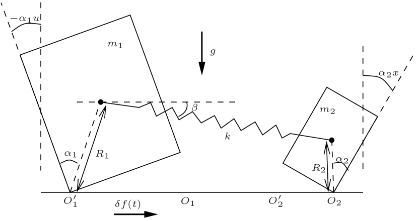
Figure 5: Two rocking blocks linked by a spring.

Both blocks are rigid, of mass $m_{i}$ and with semi–diagonal of length $R_{i}$. They are connected by a light spring, with spring constant $k$. The base is assumed to be sufficiently flat so that block $i$ rotates only about points $O_{i},O^{{}^{\prime}}_{i}$. On impact with the rigid base, neither block loses energy. Let $\alpha_{i}$ be the angle formed by the lateral side and the diagonal of each block. We then take as state variables $u$ and $x$ such that $\alpha_{1}u$ and $\alpha_{2}x$ are the angles formed by the vertical and the lateral side of each block. When there is rotation, $u$ is positive (negative) for rotation about $O_{1}$ ($O^{{}^{\prime}}_{1}$) and $x$ is positive (negative) for rotation about $O_{2}$ ($O^{{}^{\prime}}_{2}$). The spring makes an angle $\beta$ with the horizontal. As shown in [Hog89], when both blocks are slender ($\alpha_{i}<<1$), the dynamics of each is modeled by the piecewise Hamiltonian systems

$$U(u,v)=\left\{\begin{aligned} \frac{v^{2}}{2}-\frac{u^{2}}{2}+u,&\text{ if }u\geq 0\\ \frac{v^{2}}{2}-\frac{u^{2}}{2}-u,&\text{ if }u<0\end{aligned}\right.$$

and

$$X(x,y)=\left\{\begin{aligned} \frac{y^{2}}{2}-\frac{x^{2}}{2}+x,&\text{ if }x\geq 0\\ \frac{y^{2}}{2}-\frac{x^{2}}{2}-x,&\text{ if }x<0.\end{aligned}\right.$$

Each system has two critical points at $Q^{\pm}=(\pm 1,0)$, and there are two heteroclinic connections $\gamma^{\text{up/down}}$ between them, given by the energy level $U(u,v)=\frac{1}{2}$ and $X(x,y)=\frac{1}{2}$,

$$\gamma^{\text{up/down}}=\left\{(x,y)=\sigma^{\text{up/down}}(\xi),\xi\in\mathbb{R}\right\},$$

where

$$\sigma^{\text{up/down}}(\xi)=\left\{\begin{aligned} &(+\!/\!-(1-e^{-\xi}),+\!/\!-e^{-\xi})&&\text{if }\xi\geq 0\\ &(+\!/\!-(e^{\xi}-1),+\!/\!-e^{\xi})&&\text{if }\xi<0.\end{aligned}\right\}$$

These heteroclinic connections surround a region filled with a continuum of period orbits, which are given by $U(u,v)=c$ and $X(x,y)=c$, with $0<c<\frac{1}{2}$, and

$$\phi_{\mathcal{U}}(\tau;0,v)=\left\{\begin{aligned} &\bigg{(}\frac{v-1}{2}e^{\tau}-\frac{v+1}{2}e^{-\tau}+1,\\ &\quad\frac{v-1}{2}e^{\tau}+\frac{v+1}{2}e^{-\tau}\bigg{)}&&\text{if }0\leq\tau\leq\alpha^{+}(v)\\ &\bigg{(}-\frac{v-1}{2}e^{\tau-\alpha^{+}(v)}+\frac{v+1}{2}e^{-\tau+\alpha^{+}(v)}-1,\\ &\quad-\frac{v-1}{2}e^{\tau-\alpha^{+}(v)}-\frac{v+1}{2}e^{-\tau+\alpha^{+}(v)}\bigg{)}&&\text{if }\tau\alpha^{+}(v)\leq\tau\leq\alpha(v),\end{aligned}\right.$$

with $\alpha^{+}(v)$ and $\alpha(v)$ given by

$$\alpha^{+}(v) =2\int_{0}^{1-\sqrt{1-v^{2}}}\frac{1}{\sqrt{v^{2}+u^{2}-2u}}du=$$

$$=2\ln\left(\frac{1+u}{1-u}\right)$$

$$\alpha(v) =2\alpha^{+}(v),$$

(similarly for the Hamiltonian $X$). Hence conditions C.1–C.4 of §2 are satisfied.

We now assume that both blocks are identical ($\alpha_{1}=\alpha_{2}$, $R_{1}=R_{2},m_{1}=m_{2}$). This allows us to assume that the angle formed by the spring and the horizontal is small, and hence to linearize the coupling around $\beta=0$. When the blocks are subject to an external small $T$-periodic forcing given by $\delta f(t)$, the (linearized) equations that govern the system in the extended phase space are

$$\dot{u}= v$$ (6.1)

$$\dot{v}= u-\text{sgn}(u)$$

$$+k(x-u)-\delta f(s)$$

$$\dot{x}= y$$

$$\dot{y}= x-\text{sgn}(x)$$

$$+k(u-x)-\delta f(s)$$

$$\dot{s}= 1,$$

Introducing the perturbation parameter $\varepsilon$ through the reparameterization

$$\delta=\tilde{\delta}\varepsilon,\quad k=\tilde{k}\varepsilon,$$

with $\tilde{\delta}$ and $\tilde{k}$ both positive constants, and taking $f(s)=\cos(\omega s)$ ([Hog89]), these equations can be written in terms of a piecewise-smooth Hamiltonian of the form

$$H_{\varepsilon}(u,v,x,y,s)=U(u,v)+X(x,y)+\varepsilon h(u,x,s)$$ (6.2)

where $h$ is the Hamiltonian perturbation

$$h(u,x,s)=\tilde{\delta}(u+x)\cos(\omega s)+\tilde{k}\big{(}\frac{u^{2}}{2}+\frac{x^{2}}{2}-ux\big{)}.$$ (6.3)

The objects given by the critical points and heteroclinic connections of the Hamiltonian $X$, on one hand, and the periodic orbits of the Hamiltonian $U$, on the other one, give rise to the manifolds

$$\tilde{\Lambda}^{\pm}=\left\{(\phi_{\mathcal{U}}(\theta\alpha(v);0,v),\pm 1,0,s)\in\mathbb{R}^{4}\times\mathbb{T}_{T},\,\sqrt{2c_{1}}\leq v\leq\sqrt{2c_{2}},\,0\leq\theta\leq 1\right\},$$

$0<c_{1},c_{2}<\frac{1}{2}$, that are invariant for the coupled system when $\varepsilon=0$ and have $4$-dimensional heteroclinic manifolds $\tilde{\gamma}^{\text{up}}=W^{s}(\tilde{\Lambda}^{+})=W^{u}(\tilde{\Lambda}^{-})$ and $\tilde{\gamma}^{\text{down}}=W^{u}(\tilde{\Lambda}^{+})=W^{s}(\tilde{\Lambda}^{-})$.

As stated in Proposition 4.1, the invariant manifolds $\tilde{\Lambda}^{\pm}$ persist when $\varepsilon>0$ is small enough. Moreover, as shown in Proposition 5.1, the Melnikov function (5.2) provides the first order term in $\varepsilon$ of the distance of between the unstable and stable manifolds of $\tilde{\Lambda}_{\varepsilon}^{-}$ and $\tilde{\Lambda}_{\varepsilon}^{+}$, respectively. For system (6.2) this becomes

$$M(\zeta,\theta,v,s):=\int_{-\infty}^{\infty}\left(-y(t)(\tilde{\delta}\cos(\omega(s+\zeta))+\tilde{k}(x(t)-u(t)))\right)dt,$$ (6.4)

where $(x(t),y(t))=\sigma^{\text{up}}(t)$ and $u(t)=\Pi_{u}(\phi_{\mathcal{U}}(\theta\alpha(v)+t+\zeta;0,v))$.
More precisely, $M(\zeta,\theta,v,s)$ computes the first order distance between the points $\tilde{z}^{u}$ and $\tilde{z}^{s}$, given, respectively, by intersection between $W^{u}(\tilde{\Lambda}_{\varepsilon}^{-})$ and $W^{s}(\tilde{\Lambda}_{\varepsilon}^{+})$ with the line

$$\tilde{N}=\left\{\tilde{z}_{0}+l(0,0,0,1,0),\,l\in\mathbb{R}\right\}\subset\mathbb{R}^{2}\times\Sigma\times\mathbb{T}_{T},$$

where $\tilde{z}_{0}$ belongs to the intersection of $W^{u}(\tilde{\Lambda}_{0}^{-})=W^{s}(\tilde{\Lambda}_{0}^{+})$ with $\left\{x=0\right\}$ for $\varepsilon=0$, and is parametrized by

$$\tilde{z}_{0}=\tilde{z}_{0}(\zeta,\theta,v,s):=\left(\phi_{\mathcal{U}}\left(\theta\alpha(v)+\zeta;0,v\right),0,1,s+\zeta\right).$$

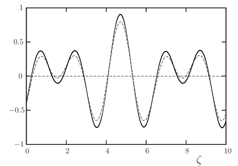
Figure 6: Melnikov function and real distance (dashed) for $v=0.48$, $\theta=s=0$ and $\varepsilon=0.01$. The real distance has been magnified by a factor of $\frac{1}{\varepsilon}$ to be compared with the Melnikov function.

In figure 6 we provide both the Melnikov function and the real distance between $\tilde{z}^{u}$ and $\tilde{z}^{s}$ for $\varepsilon=0.01$, $v=0.48$, $\theta=s=0$ when varying $\zeta$. This real distance is computed as follows. Having fixed $(\theta,v,s)$ and $\varepsilon$, for every $\zeta$ we numerically find the $y$ coordinates ($y^{u}$ and $y^{s}$) of $\tilde{z}^{u}$ and $\tilde{z}^{s}$ and subtract them. To compute $y^{s}$, we take an $\varepsilon$-neighbourhood of $y=1$ (where the unperturbed manifold intersects $x=0$) which we assume contains $y^{s}$, and use a Bolzano-like method. We consider a set of initial conditions

$$\left(\phi_{\mathcal{U}}(\theta\alpha(v)+\zeta;0,v),0,y_{i},s+\zeta\right),$$

with $y_{i}\in\left(1-O(\varepsilon),1+O(\varepsilon)\right)$, and integrate the flow forwards in time for each of them. As the stable manifold $W^{s}(\tilde{\Lambda}_{\varepsilon}^{*})$ is $4$-dimensional, it separates the space into two pieces and hence, if $\varepsilon>0$ is small enough, trajectories either escape to infinity and or return to the section $x=0$. This gives us $y_{i}$ and $y_{i+1}$ where $y_{i}$ is the largest value such that the trajectory returns to $x=0$ and $y_{i+1}$ is the smallest value such that its trajectory escapes to infinity. Hence $y^{s}\in(y_{i},y_{i+1})$ and we proceed again with this smaller interval. This is repeated until some desired tolerance is achieved.

The integration of the flow was done using an adaptative high order Runge Kutta method (RKF78) with multiple precision libraries. The number of initial conditions taken along the current interval at each iteration was $50$, and their trajectories were launched in parallel. This allowed us to compute $y^{s}$ with a tolerance of $10^{-27}$ (length of the last interval) within a reasonable time. We proceeded similarly for $y^{u}$, integrating backwards in time, also in parallel. As can be seen in figure 6, the real distance agrees very well with the value given by $M(\zeta,\theta,v,s)$ multiplied by $\varepsilon$.

Note that both the integration of the system and the computation of the Melnikov function have been done numerically. We have used neither the linearity nor the symmetry of the system, apart from the explicit expressions for $\alpha(v)$, $\phi_{\mathcal{U}}$ and $\sigma^{\text{up}}(t)$, which could easily have been computed numerically. Thus, the same techniques could easily be applied to the full nonlinear equations.

As shown in Proposition 5.1, of special interest are the zeros of the Melnikov function, which lead to zeros of the real distance between $\tilde{z}^{u}$ and $\tilde{z}^{s}$ and, hence, to heteroclinic connections. In other words, for each simple zero $\bar{\zeta}$ there exists $\zeta^{*}=\bar{\zeta}+O(\varepsilon)$ such that $\tilde{z}^{s}=\tilde{z}^{u}:=\tilde{z}^{*}$ and points $\tilde{z}^{\pm}$ satisfying

$$\lim_{t\to\pm\infty}\left|\tilde{\phi}(t;\tilde{z}^{*};\varepsilon)-\tilde{\phi}(t;\tilde{z}^{\pm};\varepsilon)\right|=0.$$

These are of the form

$$\tilde{z}^{\pm} =\left(\phi_{\mathcal{U}}(\theta\alpha(v)+\bar{\zeta};0,v),\pm 1,0,s+\zeta\right)+O(\varepsilon)$$

$$\tilde{z}^{*} =\left(\phi_{\mathcal{U}}(\theta\alpha(v)+\bar{\zeta};0,v),0,1,s+\zeta\right)+O(\varepsilon).$$

The points $\tilde{z}^{\pm}$ may be located at different energy levels on the manifolds $\tilde{\Lambda}_{\varepsilon}^{\pm}$. Their first order difference is provided in terms of the unperturbed flows by (5.18) in Proposition 5.2. In addition, (5.19) of Proposition 5.2 provides an expression for the first order difference between the average energy of the trajectories $\tilde{\phi}(\pm t;\tilde{z}^{\pm};\varepsilon)$ for $t\to\infty$.

If we compute expression (5.19) for the third and fourth positive (in $\zeta$) zeros of the Melnikov function we obtain

$$<U(\tilde{\phi}(t;\tilde{z}^{+};\varepsilon))>-<U\left(\tilde{\phi}\left(t;\tilde{z}^{-};\varepsilon\right)\right)>\simeq 0.4$$ (6.5)

for the third zero, and

$$<U(\tilde{\phi}(t;\tilde{z}^{+};\varepsilon))>-<U\left(\tilde{\phi}\left(t;\tilde{z}^{-};\varepsilon\right)\right)>\simeq-0.3$$ (6.6)

for the fourth one. Note that a positive difference implies an increase of the energy of the system while a negative one a decrease. Note the high dependence of this difference on the choice of the zero.

We now compute numerically the third and fourth zeros of the real distance in order to compute their associated heteroclinic connections and illustrate this behaviour. This is done by using a Bolzano method starting in a $\varepsilon$-neighbourhood of each zero. For each value of $\zeta$, we calculate $\tilde{z}^{u}$ and $\tilde{z}^{s}$ as explained before and calculate their difference. From the third step of the Bolzano method we use the previous computations to obtain a prediction for the next interval in $y$ where to look for $y^{s}$ (similarly for $y^{u}$), which improves the method significantly. This is done until the real zero is computed with a precision of $10^{-26}$. We find

$$\tilde{z}^{*} =(-0.11379311572593961969337806,$$

$$0.12554935975439240524029269,$$

$$0,1.11150143902429741752435119,$$

$$1.71158269885731891700238123)$$

for the third zero of the Melnikov function and

$$\tilde{z}^{*} =(0.09636673455802005569868835,$$

$$-0.21668659029422144991945461,$$

$$0,1.12033664434168488471504850,$$

$$2.85947780778602337824850186)$$

for the fourth one. Their trajectories are shown in figures 7 and 8. The initial condition $\tilde{z}^{*}$ belongs to the section $x=0$ and is used to integrate the flow forwards and backwards. Note that, due to numerical errors, the trajectory escapes after spiraling around the manifolds $\tilde{\Lambda}_{\varepsilon}^{*}$ and $\tilde{\Lambda}_{\varepsilon}^{-}$.

\begin{picture}(1.0,0.4)\put(0.0,0.35){ \begin{@subfigure}\includegraphics[angle={-90},width=216.81pt]{heteroclinic_orbit_theta0_bgam1d7.pdf} \end{@subfigure}} \put(0.5,0.35){ \begin{@subfigure}\includegraphics[angle={-90},width=216.81pt]{heteroclinic_orbit_theta0_bgam1d7_uv.pdf} \end{@subfigure}} \end{picture}

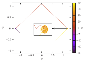
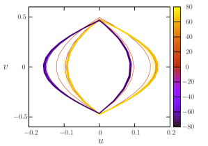
Figure 7: Trajectory close the heteroclinic point $\tilde{z}^{*}$ obtained for the third zero of the Melnikov function in figure 6. Projections onto (a) the $(u,v)$ plane and (b) the $(x,y)$ plane. The colour bar denotes time.

\begin{picture}(1.0,0.4)\put(0.0,0.35){ \begin{@subfigure}\includegraphics[angle={-90},width=216.81pt]{heteroclinic_orbit_theta0_bgam2d9.pdf} \end{@subfigure}} \put(0.5,0.35){ \begin{@subfigure}\includegraphics[angle={-90},width=216.81pt]{heteroclinic_orbit_theta0_bgam2d9_uv.pdf} \end{@subfigure}} \end{picture}

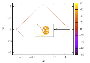
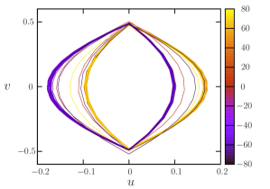
Figure 8: Same as in figure 7 for the fourth zero of the Melnikov function in figure 6.

In order to validate (6.5) and (6.6), we show in figure 9 the Hamiltonian $U$ evaluated along the trajectories. Note that the transition from $\tilde{\Lambda}_{\varepsilon}^{-}$ to $\tilde{\Lambda}_{\varepsilon}^{+}$ is very fast and the trajectories spend most of the time close to the invariant manifolds until they escape, both forwards and backwards in time. In the same figure, we show the average functions

$$\frac{1}{t}\int_{0}^{t}U\left(\tilde{\phi}\left(r;\tilde{z}^{*};\varepsilon\right)\right)dr.$$ (6.7)

The difference between the limiting values of the averages is shown magnified in figure 10 for $t\to\infty$ and $t\to-\infty$. There is good agreement with the values given in (6.5) and (6.6), multiplied by $\varepsilon$.

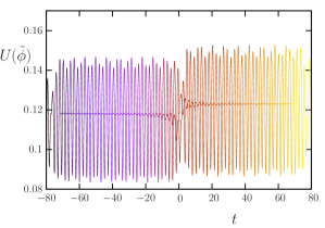
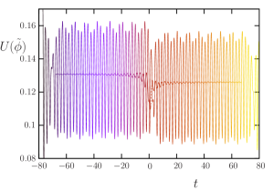
Figure 9: Hamiltonian $U$ evaluated along the trajectory $\tilde{\phi}(t;\tilde{z}^{*};\varepsilon)$ for (a) the third and (b) the fourth zeros of the Melnikov function in figure 6. The average function (6.7) is also shown.

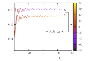
Figure 10: Average function (6.7) for the trajectories shown in figures 7 and 8 (magnification of figure 9). The colour bar denotes $t$. Note that the horizontal axis denotes $|t|$, for better comparison of the limiting values.

We now study the effect of varying $\theta$ whilst keeping $v$ and $s$ constant. In figure 11 we show the values (dotted) of (5.19) for different values of $\theta$, for the third and fourth zeros of the Melnikov function. In the same figure we show the result of computing the heteroclinic point $\tilde{z}^{*}$ and proceeding as before to compute the difference between the limiting averages of the asymptotic dynamics. The agreement is good.

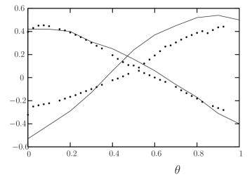
Figure 11: Values (dotted) of (5.19) as a function of $\theta$ for $v=0.48$ and $s=0$ for the third and fourth positive zeros of the Melnikov function compared with the difference computed as in figure 10 for $\varepsilon=0.01$ (lines).

Finally, we study the first order difference given in (5.19) when varying $v$ and $\theta$, whilst keeping $s$ constant, for different zeros of the Melnikov function. For each $(\theta,v)$ we compute the Melnikov function, and for each zero we compute expression (5.19). The resulting values are shown on the left of figures 12-14 for the first three positive zeros of the Melnikov function, which are shown on the right of these figures. Note that, in figure 12 (right), there is a discontinuity curve (in black) corresponding to a relabelling of zeros. Positive values in the left-hand figures lead to an increase of energy in one iteration of the scattering map $S^{\text{up}}$, while negative ones lead to a decrease. For the same coordinates $(\theta,v)$, different zeros of the Melnikov function have different behaviours. When combining this with the same study for the map $S^{\text{down}}$ associated with the lower heteroclinic connection, these results can be used to find suitable candidate trajectories exhibiting diffusion.

Figure 12: (left) First order difference between the average energy of the trajectories $\tilde{\phi}(\pm t;\tilde{z}^{\pm};\varepsilon)$ when $t\to\infty$ for the first positive zero of the Melnikov function. (right) First positive zeros of the Melnikov function.

Figure 13: Same as figure 12 for the second zero of the Melnikov function.

Figure 14: Same as figure 12 for the third zero of the Melnikov function.

7 Conclusions

We have considered a non-autonomous dynamical system formed by coupling two piecewise-smooth systems in $\mathbb{R}^{2}$ through a non-autonomous periodic perturbation, leading to a two and a half degrees of freedom piecewise-smooth Hamiltonian system with two switching manifolds.
We have studied the dynamics around one of the heteroclinic orbits of one of the piecewise-smooth systems, which is captured by $3$-dimensional invariant manifolds with stable and unstable manifolds. In the unperturbed case, these stable and unstable manifolds coincide, leading to the existence of two $4$-dimensional heteroclinic manifolds connecting the two invariant manifolds. These heteroclinic manifolds are foliated by heteroclinic connections between $C^{0}$ tori located at the same levels of energy in both invariant manifolds.
By means of the impact map we have proved the persistence of these objects under perturbation. In addition, we have provided sufficient conditions for the existence of transversal heteroclinic intersections through the existence of simple zeros of Melnikov-like functions, thereby extending some of the results given in [DdlLS06].
These heteroclinic manifolds allow us to define the scattering map, which links asymptotic dynamics in the invariant manifolds through heteroclinic connections. First order properties of this map provide sufficient conditions for the asymptotic dynamics to be located in different energy levels in the perturbed invariant manifolds. Hence this is an essential tool for the construction of a heteroclinic skeleton which, when followed, can lead to the existence of Arnol’d diffusion: trajectories that, on large time scales, destabilize the system by further accumulating energy.
Finally we have validated all the theoretical results in this paper with detailed numerical computations of a mechanical system with impacts, formed by the linkage of two rocking blocks with a spring. Future work should include the study of the concatenation of the scattering map in order to construct diffusion trajectories.

References

- [Arn64] V. Arnol’d. Instability of dynamical systems with several degrees of freedom. Soviet Math., 5:581–585, 1964.
- [BBB02] M. Berti, L. Biasco, and P. Bolle. Optimal stability and instability results for a class of nearly integrable Hamiltonian systems. Atti Accad. Naz. Lincei Cl. Sci. Fis. Mat. Natur. Rend. Lincei (9) Mat. Appl., 13(2):77–84, 2002.
- [BBB03] M. Berti, L. Biasco, and P. Bolle. Drift in phase space: a new variational mechanism with optimal diffusion time. J. Math. Pures Appl. (9), 82(6):613–664, 2003.
- [Ber02] M. Berti. Arnol’d diffusion: a functional analysis approach. In Symmetry in nonlinear mathematical physics, Part 1, 2 (Kyiv, 2001), volume 2 of Pr. Inst. Mat. Nats. Akad. Nauk Ukr. Mat. Zastos., 43, Part 1, pages 712–719. Natsīonal. Akad. Nauk Ukraïni Īnst. Mat., Kiev, 2002.
- [Ber10] P. Bernard. Arnold’s diffusion: from the a priori unstable to the a priori stable case. In Proceedings of the International Congress of Mathematicians. Volume III, pages 1680–1700, New Delhi, 2010. Hindustan Book Agency.
- [BKZ11] P. Bernard, V. Kaloshin, and K. Zhang. Arnol’d diffusion in arbitrary degrees of freedom and crumpled 3-dimensional normally hyperbolic invariant cylinders. 2011. Preprint.
- [CG94] L. Chierchia and G. Gallavotti. Drift and diffusion in phase space. Ann. Inst. H. Poincaré Phys. Théor., 60(1):144, 1994.
- [Che08] C-Q. Cheng. Variational methods for the problem of Arnold diffusion. In Hamiltonian dynamical systems and applications, NATO Sci. Peace Secur. Ser. B Phys. Biophys., pages 337–365. Springer, Dordrecht, 2008.
- [Che10] C-Q. Cheng. Variational construction of diffusion orbits for positive definite Lagrangians. In Proc. Inter. Cong. Math., volume 3, pages 1714–1728, New Delhi, 2010. Hindustan Book Agency.
- [CK09] W–S. Choi, D–O. Kim, K–B. Park, J–M. Noh and W–J. Lee. Evaluation of the behaviour of stacked blocks subject to a harmonic forcing Proc. 17th Int. Conf. Nuclear Eng., 2:75–80, 2009.
- [CY04] C-Q. Cheng and J. Yan. Existence of diffusion orbits in a priori unstable Hamiltonian systems. J. Differential Geom., 67(3):457–517, 2004.
- [DdlLS00] A. Delshams, R. de la Llave and T.M. Seara. A geometric approach to the existence of orbits with unbounded energy in generic periodic perturbations by a potential of generic geodesic flows of . Comm. Math. Phys., 209:353–392, 2000.
- [DdlLS06] A. Delshams, R. de la Llave and T.M. Seara. A geometric mechanism for diffusion in Hamiltonian systems overcoming the large gap problem: Heuristics and rigorous verification on a model. Mem. Am. Math. Soc., 179, 2006.
- [DdlLS08] A. Delshams, R. de la Llave and T.M. Seara. Geometric properties of the scattering map of a normally hyperbolic invariant manifold. Adv. in Math., 217:1096–1153, 2008.
- [DGdlLS08] A. Delsahms, M. Gidea, R. de la Llave, and T.M. Seara. Geometric approaches to the problem of instability in Hamiltonian systems. An informal presentation. In Hamiltonian dynamical systems and applications, NATO Sci. Peace Secur. Ser. B Phys. Biophys., pages 285–336. Springer, Dordrecht, 2008.
- [DuLi12] Z. Du and Y. Li. Bifurcation of periodic orbits with multiple crossings in a class of planar Filippov systems. Math. Comp. Modelling 55:1072–1082, 2012.
- [Fen72] N. Fenichel. Persistence and smoothness of invariant manifolds for flows. Indiana Univ. Math. J., 21:193–226, 1971/1972.
- [Fen74] N. Fenichel. Asymptotic stability with rate conditions. Indiana Univ. Math. J., 23:1109–1137, 1973/74.
- [Fen77] N. Fenichel. Asymptotic stability with rate conditions. II. Indiana Univ. Math. J., 26:81–93, 1977.
- [GdlL06] M. Gidea and R. de la Llave. Topological methods in the instability problem of Hamiltonian systems. Discr. Contin. Dyn. Syst., 14(2):295–328, 2006.
- [GHS12] A. Granados, S.J. Hogan and T.M. Seara. The Melnikov method and subharmonic orbits in a piecewise smooth system. SIAM J. Appl. Dyn. Syst., 11:801–830, 2012.
- [Gra12] A. Granados. Local and global phenomena in piecewise-defined systems: from big bang bifurcations to splitting of heteroclinic manifolds. PhD thesis, UPC, September 2012.
- [GST11] M. Guardia, T.M. Seara and M.A. Teixeira. Generic bifurcations of low codimension of planar Filippov systems. J. Differential Equations, 250:1967–2023, 2011.
- [GH83] J. Guckenheimer and P.J. Holmes Nonlinear Oscillations, Dynamical Systems and Bifurcations of Vector Fields. 4th ed., Appl. Math. Sci. 42, Springer, New York, 1983.
- [Hog89] S.J. Hogan. On the dynamiccs of rigid block motion under harmonic forcing. Proc. Roy. Soc. Lond. A, 425:441–476, 1989.
- [Hou63] G.W. Housner. The behaviour of inverted pendulum structures during earthquakes. Bull. Seism. Soc. Am., 53:403–417, 1963.
- [HP70] M.W. Hirsch and C.C. Pugh. Stable manifolds and hyperbolic sets. In S. Chern and S. Smale, editors, Global Analysis (Proc. Sympos. Pure Math., Vol. XIV, Berkeley, Calif., 1968), pages 133–163, Providence, R.I., 1970. Amer. Math. Soc.
- [HPS77] M.W. Hirsch, C.C. Pugh and M. Shub. Invariant Manifolds, volume 583 of Lecture Notes in Mathematics. Springer-Verlag, 1977.
- [FGKR11] J. Fejoz, V. Kaloshin, M. Guardia and P. Rodan Diffusion along mean motion resonance in the restricted planar three-body problem. 2011. Preprint.
- [KL08a] V. Kaloshin and M. Levi. An example of Arnold diffusion for near-integrable Hamiltonians. Bull. Amer. Math. Soc. (N.S.), 45(3):409–427, 2008.
- [KL08b] V. Kaloshin and M. Levi. Geometry of Arnold diffusion. SIAM Rev., 50(4):702–720, 2008.
- [KZ12] V. Kaloshin and K. Zhang. A strong form of arnold diffusion for two and a half degrees of freedom. 2012. Preprint.
- [KPC12] A.N. Kounadis, G.J. Papadopoulos and D.M. Cotsovos. Overturning instability of a two-rigid block system under ground excitation. Z. Angew. Math. Mech. 92: 536–557, 2012
- [Kov10] A. Kovaleva. The Melnikov criterion of instability for random rocking dynamics of a rigid block with an attached secondary structure. Nonlinear Analysis: Real World Applications 11: 472–479, 2010.
- [KKY97] M. Kunze, T. Küpper and J. You. On the application of KAM theory to discontinuous dynamical systems. J. Differential Equations, 139:1–21, 1997.
- [Kuz04] Y. Kuznetsov. Elements of Applied Bifurcation Theory. Springer, 2004. Third edition.
- [Lev91] M. Levi. Quasiperiodic motions in superquadratic time-periodic potentials. Comm. Math. Phys., 143:43–83, 1991.
- [ML12] O. Makarenkov and J.S.W. Lamb. Dynamics and bifurcations of nonsmooth systems: A survey. Physica D, 241:1826–1844, 2012.
- [Mat02] J. Mather. Arnold diffusion i: announcement of results. 2002. Preprint.
- [Mel63] V.K. Melnikov On the stability of the center for time–periodic perturbations Trans. Moscow Math. Soc., 12:1–56, 1963.
- [PLC08] F. Peña, P.B. Lourenço and A. Campos–Costa. Experimental dyanmic behaviour of free–standing multi–block structures under seismic loadings. J. Earthquake Eng., 12:953–979, 2008.
- [RdlL02] T.M-Seara R. de la LLave, M. Gidea. General mechanisms of diffusion in hamiltonian systems. 2002. Preprint.
- [SK84] P.D. Spanos and A.–S. Koh. Rocking of rigid blocks due to harmonic shaking. J. Eng. Mech. ASCE, 110:1627–1642, 1984.
- [SRP01] P.D. Spanos, P.C. Roussis and N.P.A. Politis. Dynamic analysis of stacked rigid blocks. Soil Dyn. Earthquake Eng 21:559–578, 2001
- [Tre04] D. Treschev. Evolution of slow variables in a priori unstable Hamiltonian systems. Nonlinearity, 17(5):1803–1841, 2004.
- [Tre12] D. Treschev. Arnold diffusion far from strong resonances in multidimensional a priori unstable Hamiltonian systems. Nonlinearity, 25(9):2717–2757, 2012. systems.
- [YCP80] C.–S. Yim, A.K. Chopra and J. Penzien. Rocking response of rigid blocks to earthquakes. Earthquake Engng. Struct. Dyn., 8:565–587, 1980.