A model for the nonautonomous Hopf bifurcation

Abstract

Inspired by an example of Grebogi et al [1], we study a class of model systems which exhibit the full two-step scenario for the nonautonomous Hopf bifurcation, as proposed by Arnold [2]. The specific structure of these models allows a rigorous and thorough analysis of the bifurcation pattern. In particular, we show the existence of an invariant ‘generalised torus’ splitting off a previously stable central manifold after the second bifurcation point.

The scenario is described in two different settings. First, we consider deterministically forced models, which can be treated as continuous skew product systems on a compact product space. Secondly, we treat randomly forced systems, which lead to skew products over a measure-preserving base transformation. In the random case, a semiuniform ergodic theorem for random dynamical systems is required, to make up for the lack of compactness.

2010 Mathematics Subject Classification. Primary 39A28, 37H20, 34C23

Keywords: Skew Products, Random Dynamical Systems, Nonautonomous Hopf Bifurcation.

1 Introduction

External forcing often leads to important changes in the bifurcation pattern of dynamical systems. Yet, despite the relevance of this issue in many applications and significant progress over the last decades (see [2, 4, 5] for an overview and [6, 7, 8, 9] for some recent advances), our understanding of non-autonomous bifurcations is still limited. Maybe the most prominent example for this is the non-autonomous Hopf bifurcation [2, 10, 11]. Here, external forcing can lead to the separation of the complex-conjugate eigenvalues [12]. This gives rise to a two-step bifurcation scenario, in which an invariant ‘torus’ splits off a previously stable central manifold [2, Chapter 9.4]. However, so far this phenomenological description is mainly based on numerical evidence, and up to date there exist no non-trivial examples for which this bifurcation pattern can be described analytically. In particular, it is an open problem to describe the structure of the split-off ‘torus’. Earlier simulations suggested that this structure is simple, in the sense that the intersection with each fibre of the product space is a topological circle [12]. However, later numerical studies based on refined algorithms indicate that more complicated structures may appear as well [13] .

The aim of this article is to give a description of the non-autonomous Hopf bifurcation in a class of model systems which is accessible to a rigorous analysis, but at the same time allows for highly non-trivial dynamics. For the sake of a simpler exposition we focus on discrete-time systems, although continuous-time analogues are easy to derive (see Section 6). In the situation we consider, the split-off ‘torus’ consists of a topological circle in each fibre and hence belongs to the simpler case described above, but this should not be taken as an indication for the general case.

We study parametrised families of skew products

(1.1) $$f_{\beta}\ :\ \Theta\times\mathbb{R}^{2}\to\Theta\times\mathbb{R}^{2}\quad,\quad(\theta,v)\mapsto(\gamma(\theta),f_{\beta,\theta}(v))$$

with fibre maps

(1.2) $$f_{\beta,\theta}(v)\ =\ \left\{\begin{array}[]{cl}h(\beta\|v\|)A(\theta)\frac{v}{\|v\|}&\textrm{if }v\neq 0\\ \\ 0&\textrm{if }v=0\end{array}\right.\quad,$$

where $\|\cdot\|$ denotes the Euclidean norm on $\mathbb{R}^{2}$ and $\beta\in\mathbb{R}^{+}$ is the bifurcation parameter. Maps of this type were introduced by Grebogi et al [1] as examples for the existence of strange non-chaotic attractors. A first step in their rigorous analysis was made in [14], and our results on continuous systems can be seen as an extension of this work (see Theorem 1.1 and Section 4).

We consider two different settings. For modelling deterministic forcing, we assume that

• $\Theta$ is a compact metric space and $\gamma$ is a homeomorphism;

• $h:\mathbb{R}^{+}\to\mathbb{R}^{+}$ is $\mathcal{C}^{2}$, strictly increasing, strictly concave, bounded and satisfies $h(0)=0$ and $h^{\prime}(0)=1$;

• $A:\Theta\to\textrm{SL}(2,\mathbb{R})$ is continuous.

In order to give a concise description of the bifurcation pattern in this setting, we concentrate on the behaviour of the global attractor of $f_{\beta}$. By rescaling if necessary, we may and will assume

(1.3) $$\sup_{x\geq 0}h(x)\ \leq\ \left(\max_{\theta\in\Theta}\|A(\theta)\|\right)^{-1}\ .$$

Consequently $f_{\beta}(\Theta\times\mathbb{R}^{2})\subseteq\Theta\times\overline{B_{1}(0)}$, so that the global attractor can be defined as

(1.4) $$\mathcal{A}_{\beta}\ =\ \bigcap_{n\in\mathbb{N}}f_{\beta}^{n}\left(\Theta\times\overline{B_{1}(0)}\right)\ .$$

We let $\mathcal{A}_{\beta}(\theta)=\{x\in\mathbb{R}^{2}\mid(\theta,x)\in\mathcal{A}_{\beta}\}$ and use the analogous notation for other subsets of product spaces. As we will see, the particular structure of (1.1) implies that $\mathcal{A}_{\beta}$ has the form

(1.5) $$\mathcal{A}_{\beta}\ =\ \left\{\left(\left.\theta,rv(\alpha)\right)\ \right|\ \theta\in\Theta,\ \alpha\in[0,1),\ r\in[0,r_{\beta}(\theta,\alpha)]\right\}\ ,$$

where $v(\alpha)=(\cos(2\pi\alpha),\sin(2\pi\alpha))^{t}$ and $r_{\beta}:\Theta\times\mathbb{R}\to[0,1]$ is an upper semi-continuous function which is $\frac{1}{2}$-periodic in the second variable. The bifurcation parameters in the above system are determined by the maximal exponential expansion rate of the cocycle $(\gamma,A)$. The latter is given by the maximal Lyapunov exponent of $A$,

(1.6) $$\lambda_{\mathrm{max}}(A)\ =\ \sup_{\theta\in\Theta}\limsup_{n\to\infty}\frac{1}{n}\log\|A_{n}(\theta)\|\ ,$$

where $A_{n}(\theta)=A(\gamma^{n-1}\theta)\circ\ldots\circ A(\theta)$.

Theorem 1.1.

Suppose $(f_{\beta})_{\beta\in\mathbb{R}^{+}}$ is of the form (1.1) and satisfies conditions (D1)–(D3). Let

$$\beta_{1}\ :=\ e^{-\lambda_{\mathrm{max}}}\quad\textrm{and}\quad\beta_{2}\ :=\ e^{\lambda_{\mathrm{max}}}\ .$$

Then the following hold.

• If $\beta<\beta_{1}$, then the global attractor $\mathcal{A}_{\beta}$ is equal to $\Theta\times\{0\}$.

• If $\beta_{1}<\beta<\beta_{2}$, then there exists at least one $\theta^{*}\in\Theta$ such that $\mathcal{A}_{\beta}(\theta^{*})$ is a line segment of positive length.

• If $\beta>\beta_{2}$, then for all $\theta\in\Theta$ the set $\mathcal{A}_{\beta}(\theta)$ is a closed topological disk and depends continuously on $\theta$. In other words, the function $r_{\beta}$ is strictly positive and continuous.

  Further, the compact $f_{\beta}$-invariant set

  (1.7) $$\mathcal{T}_{\beta}\ =\ \partial\mathcal{A}_{\beta}\ =\ \left\{\left(\left.\theta,r_{\beta}(\theta,\alpha)v(\alpha)\right)\ \right|\ \theta\in\Theta,\ \alpha\in[0,1)\right\}\$$

  is the global attractor outside $\Theta\times\{0\}$, in the sense that

  $$\mathcal{T}_{\beta}\ =\ \bigcap_{n\in\mathbb{N}}f^{n}_{\beta}\left(\Theta\times\left(\overline{B_{1}(0)}\setminus B_{\delta}(0)\right)\right)$$

  for all sufficiently small $\delta>0$.

Remark 1.2.

• Note that if $\lambda_{\mathrm{max}}(A)=0$, case (b) in the theorem is void since then $\beta_{1}=\beta_{2}$.

• In the intermediate region $\beta_{1}<\beta<\beta_{2}$, as well as for the critical cases $\beta=\beta_{1}$ and $\beta=\beta_{2}$, a great variety of dynamical behaviour is possible. In particular this behaviour is not uniform for all orbits, and given two $\gamma$-invariant measures $m_{1}$ and $m_{2}$ on $\Theta$ the typical dynamics with respect to $m_{1}$ and $m_{2}$ may be very different. Therefore, the feasible approach in this parameter regime is to fix a $\gamma$-invariant ergodic measure $m$ on the base $\Theta$ and to describe the structure of $\mathcal{A}_{\beta}(\theta)$ and other relevant properties of the system for $m$-almost every $\theta\in\Theta$.

  However, it turns out that for such an $m$-dependent description the topological structure on $\Theta$ provides no additional information whatsoever. Hence, all the related questions can directly be addressed in the purely measure-theoretic setting of random dynamical systems. In our context, this means that we can apply the random analogue to Theorem 1.1, which is given by Theorem 1.3 below, to obtain further information about the $m$-typical behaviour. See Remark 1.4(d) for details. In a similar way, further information on the critical parameters is provided by Proposition 1.5 below.

• The focus on the global attractor $\mathcal{A}_{\beta}$ and the sets $\mathcal{A}_{\beta}(\theta)$ in the above statement corresponds to the concept of pullback attractors in random dynamical systems. It describes the behaviour of trajectories coming from $-\infty$ in time. The complementary point of view is to study forward dynamics, meaning the asymptotic behaviour of trajectories $f_{\beta}^{n}(\theta,v)$ as $n$ goes to $+\infty$. In situations (a) and (c) of the above theorem, information about the forward dynamics can be derived easily. In part (a), we have

  (1.8) $$\lim_{n\rightarrow\infty}f_{\beta,\theta}^{n}(v)\ =\ 0\quad\textrm{for all }(\theta,v)\in\Theta\times\mathbb{R}^{2}\ ,$$

  whereas in part (c) we have

  (1.9) $$\lim_{n\rightarrow\infty}d\left(f^{n}_{\beta}(\theta,v),\mathcal{T}_{\beta}\right)\ =\ 0\quad\textrm{for all }(\theta,v)\in\Theta\times(\mathbb{R}^{2}\setminus\{0\})\ .$$

  In particular, all accumulation points of trajectories outside of $\Theta\times\{0\}$ are contained in $\mathcal{T}_{\beta}$.

  In the intermediate region $\beta_{1}<\beta<\beta_{2}$, as well as for the critical parameters, the situation is more intricate and some differences appear between forward and pullback dynamics. Again, the picture may depend on a $\gamma$-invariant measure in the base which serves as a reference. If the cocycle is hyperbolic with respect to this measure, a random two-point attractor appears in the intermediate parameter regime. This attractor also survives the second bifurcation. Consequently, for $\beta>\beta_{2}$ the forward dynamics do not ‘see’ the whole ‘torus’ $\mathcal{T}_{\beta}$, but only the two-point attractor which is embedded in $\mathcal{T}_{\beta}$. We refer to Theorem 1.3 on random forcing below for further details.

• The most important property of the models in (1.1) is the fact that the fibre maps send lines passing through the origin to such lines again. As a consequence, the map written in polar coordinates becomes a double skew product (see Section 3.1), a fact which will be crucial for our analysis. Yet, the fact that the cocycle $A$ can be chosen arbitrarily allows for a great variety of dynamical behaviour when $\beta>\beta_{2}$. On the one hand, $A$ could simply be a constant rotation matrix with angle $\rho$. In this case $\beta_{1}=\beta_{2}$ and the projective action of $A$, which is equivalent to the action of $f_{\beta}$ on $\mathcal{T}_{\beta}$ is typically minimal. On the other hand, we can choose $A$ to be a uniformly hyperbolic $\textrm{SL}(2,\mathbb{R})$-cocycle, which leads to $\beta_{1}<\beta_{2}$ and attractor-repeller dynamics on $\mathcal{T}_{\beta}$. A mixture of these two types occurs when $A$ has non-uniformly hyperbolic dynamics and the projective action is minimal (see [15] for examples of this type). Then the dynamics on $\mathcal{T}_{\beta}$ are minimal, and thus resemble an irrational rotation from the topological point of view, but they are of attractor-repeller type from the measurable point of view.

As indicated by the preceding remark, the second main goal of this article is to derive a random analogue of Theorem 1.1 in the context of random dynamical systems. The motivation for this is two-fold. First, there is the obvious intrinsic interest in random forcing processes, which are modelled in a purely measure-theoretic setting. Secondly, as mentioned above, even in the topological setting the description of the typical dynamical behaviour at intermediate or critical parameters depends on the choice of a reference measure on the base. Hence, the consideration of measure-preserving driving processes is required as well, in order to gain a better understanding of deterministic forcing.

In order to model random forcing, we make the following assumptions.

• $(\Theta,\mathcal{B},m,\gamma)$ is a measure preserving dynamical system, i.e. $\gamma:\Theta\to\Theta$ is a bi-measurable bijection and $m$ is an ergodic $\gamma$-invariant probability measure;

• $h:\mathbb{R}^{+}\to\mathbb{R}^{+}$ is $\mathcal{C}^{2}$, strictly increasing, strictly concave, bounded and satisfies $h(0)=0$ and $h^{\prime}(0)=1$.

• $A:\Theta\to\textrm{SL}(2,\mathbb{R})$ is measurable and bounded.

Since in this setting there is no topological structure on $\Theta$, and consequently $\mathcal{A}_{\beta}$ has no global topological structure either, we concentrate on the structure of $\mathcal{A}_{\beta}$ on typical fibres. Note that $\mathcal{A}_{\beta}$ again has the form given by (1.5), where now $r_{\beta}:\Theta\times\mathbb{R}\to\mathbb{R}^{+}$ is a measurable function which is $\frac{1}{2}$-periodic and upper semi-continuous in the second variable. This time, the bifurcation parameters are determined by the Lyapunov exponent of the cocycle $(\gamma,A)$ with respect to $m$, which is defined as

(1.10) $$\lambda_{m}(A)\ =\ \lim_{n\to\infty}\frac{1}{n}\int_{\mathbb{T}^{1}}\log\|A_{n}(\theta)\|\ dm(\theta)\ .$$

Note that the limit exists by subadditivity.

Our second main result provides a description of the nonautonomous Hopf bifurcation in this random setting, where it is also possible to give more details on the intermediate parameter region. For the application to the deterministic models we refer to Remark 1.4(d) below. In contrast to Theorem 1.1, we now provide details on both forward and pullback dynamics. The reason is that there are important differences between the two viewpoints, in particular when $\beta_{1}\neq\beta_{2}$.

Theorem 1.3.

Suppose $(f_{\beta})_{\beta\in\mathbb{R}^{+}}$ is of the form (1.1) and satisfies conditions (R1)–(R3). Let

$$\beta_{1}^{m}\ :=\ e^{-\lambda_{m}(A)}\quad\textrm{and}\quad\beta_{2}^{m}\ :=\ e^{\lambda_{m}(A)}\ .$$

Then there exists a $\gamma$-invariant set $\Theta_{0}\subseteq\Theta$ of full measure, such that for all $\theta\in\Theta_{0}$ the following hold.

• If $\beta<\beta^{m}_{1}$, then $\mathcal{A}_{\beta}(\theta)=\{0\}$ and

  (1.11) $$\lim_{n\rightarrow\infty}f^{n}_{\beta,\theta}(v)\ =\ 0\quad\textrm{ for all }v\in\mathbb{R}^{2}\ .$$

• If $\beta_{1}^{m}<\beta<\beta_{2}^{m}$, then the set $\mathcal{A}_{\beta}(\theta)$ is a line segment of positive length. More precisely, there exist measurable functions $\alpha_{u},\alpha_{s}:\Theta_{0}\to[0,\frac{1}{2})$, not depending on $\beta$, such that $r_{\beta}(\theta,\alpha)>0$ if and only if $\alpha=\alpha_{u}(\theta)$ and we have

  (1.12) $$\mathcal{A}_{\beta}(\theta)\ =\ \left\{rv(\alpha_{u}(\theta))\mid|r|\leq r_{\beta}(\theta,\alpha_{u}(\theta))\right\}\ ,$$

  and the graph of the set-valued function

  (1.13) $$\Psi_{\beta}(\theta)\ =\ \left\{\pm r_{\beta}(\theta,\alpha_{u}(\theta))v(\alpha_{u}(\theta))\right\}$$

  is a random two-point forward attractor with domain of attraction

  $$\mathcal{D}\ =\ \{(\theta,v)\mid\theta\in\Theta_{0},v\in\mathbb{R}^{2}\setminus(\mathbb{R}v(\alpha_{s}(\theta))\}\ ,$$

  in the sense that

  (1.14) $$\lim_{n\to\infty}d\left(f^{n}_{\beta,\theta}(v),\Psi_{\beta}(\gamma^{n}\theta)\right)\ =\ 0\$$

  for all $(\theta,\alpha)\in\mathcal{D}$.

• If $\beta>\beta_{2}^{m}$, then the map $\alpha\mapsto r_{\beta}(\theta,\alpha)$ is strictly positive and continuous. The set $\mathcal{T}_{\beta}$ defined by

  (1.15) $$\mathcal{T}_{\beta}(\theta)\ =\ \partial\mathcal{A}_{\beta}(\theta)\ =\ \left\{\left.r_{\beta}(\theta,\alpha)v(\alpha)\ \right|\alpha\in[0,1)\right\}$$

  is the global pullback attractor outside $\Theta\times\{0\}$. More precisely, for all $\delta>0$ there exists an $f_{\beta}$-forward invariant random compact set $\mathcal{K}_{\beta,\delta}$ which contains $\Theta_{0}\times\left(\overline{B_{1}(0)}\setminus B_{\delta}(0)\right)$ and satisfies

  $$\mathcal{T}_{\beta}(\theta)\ =\ \bigcap_{n\in\mathbb{N}}f^{n}_{\beta,\gamma^{-n}\theta}\left(\mathcal{K}_{\beta,\delta}(\gamma^{-n}\theta)\right)\ .$$

  When $\lambda_{m}(A)>0$, the random forward attractor $\Psi_{\beta}$ given by (1.13) still exists, with $\Psi_{\beta}(\theta)\subseteq\mathcal{T}_{\beta}(\theta)$, and (1.14) remains true.

Remark 1.4.

• As before, case (b) of the theorem is void if $\beta_{1}^{m}=\beta_{2}^{m}$.

• Note that for $\beta_{1}^{m}<\beta<\beta_{2}^{m}$, the attractor $\Psi_{\beta}$ given by (1.13) consists exactly of the endpoints of the segment $\mathcal{A}_{\beta}(\theta)$ on each fibre.

• If $\beta_{1}^{m}<\beta_{2}^{m}$, then the statements on $\Psi_{\beta}$ can be interpreted in the way that this attractor persists throughout the whole parameter range (if $\beta<\beta_{1}^{m}$ it coincides with $\Theta\times\{0\}$ by definition) and attracts almost all initial conditions with respect to $m$ and the Lebesgue measure on $\mathbb{R}^{2}$.

• When $\gamma$ is a homeomorphism of a compact metric space $\Theta$ as in Theorem 1.1, we denote by $\mathcal{M}(\gamma)$ the set of $\gamma$-invariant ergodic probability measures on $\Theta$. As mentioned, we can apply Theorem 1.3 and Proposition 1.5 below for any fixed reference measure $m\in\mathcal{M}(\gamma)$ on the base. As a straightforward consequence of the semiuniform sub-multiplicative ergodic theorem (see Theorem 2.5), we have

  (1.16) $$\lambda_{\mathrm{max}}(A)\ =\ \sup_{m\in\mathcal{M}(\gamma)}\lambda_{m}(A)\ .$$

  Therefore $\beta_{1}\leq\beta_{1}^{m}\leq\beta_{2}^{m}\leq\beta_{2}$. However, due to compactness of $\mathcal{M}(\gamma)$, there always exists at least one $\hat{m}\in\mathcal{M}(\gamma)$ with $\lambda_{\hat{m}}(A)=\lambda_{\mathrm{max}}(A)$ and thus $\beta_{1}^{\hat{m}}=\beta_{1}$ and $\beta_{2}^{\hat{m}}=\beta_{2}$. When $\beta_{1}<\beta<\beta_{2}$, then this means in particular that $\hat{m}$-typical fibres are line segments of positive length and the typical dynamics with respect to $\hat{m}$ are governed by a two-point attractor $\Psi_{\beta}$ given by (1.13). Theorem 1.1(b) is a direct consequence of this.

• Note that the full measure set $\Theta_{0}\subseteq\Theta$ in the above statement is fixed and does not depend on the parameter $\beta$. Obtaining this $\beta$-independence will require some additional work, but since the parameter set is uncountable this is clearly stronger than just showing that all statements hold $m$-a.s. for all parameters $\beta$, but allowing the exceptional set to change with $\beta$.

For the three non-critical parameter regions described above, the picture provided by Theorem 1.3 can be considered rather complete. In contrast to this, the two critical parameters $\beta_{1}^{m}$ and $\beta_{2}^{m}$ are more difficult to treat, and there are some questions which we have to leave open here (see Questions 1.6). Nevertheless, the following proposition provides at least some information, both on pullback and forward dynamics.

Proposition 1.5.

Under the assumptions of Theorem 1.3, the set $\Theta_{0}$ can be chosen such that for all $\theta\in\Theta_{0}$ the following hold.

• If $\beta=\beta^{m}_{1}<\beta^{m}_{2}$, then $\mathcal{A}_{\beta}(\theta)=\{0\}$ and there exists a set $J=J(\theta)\subseteq\mathbb{N}$ of asymptotic density $0$ such that

  (1.17) $$\lim_{\begin{subarray}{c}n\to\infty\\ n\notin J(\theta)\end{subarray}}\|f^{n}_{\beta,\theta}(v)\|\ =\ 0\quad\textrm{for all }v\in\mathbb{R}^{2}\ .$$

• If $\beta=\beta_{1}^{m}=\beta_{2}^{m}$, then $\mathcal{A}_{\beta}(\theta)$ is not a topological disk. More precisely, there exists $\alpha=\alpha(\theta)$ such that $r_{\beta}(\theta,\alpha(\theta))=0$. Further,

  (1.18) $$\lim_{n\rightarrow\infty}\frac{1}{n}\sum_{i=0}^{n-1}\|f^{i}_{\beta,\theta}(v)\|\ =\ 0\quad\text{for all }v\in\mathbb{R}^{2}\ .$$

• If $\beta_{1}^{m}<\beta=\beta_{2}^{m}$, then the statement of Theorem 1.3(b) holds without any modifications.

Questions 1.6.

• In the situation of Theorem 1.1, does $\mathcal{A}_{\beta}=\Theta\times\{0\}$ still hold if $\beta=\beta_{1}$? If not, is this always true when $\gamma$ is uniquely ergodic?

• If the answer to (a) is negative, is it at least true that for $\gamma$ uniquely ergodic and $\beta=\beta_{1}$ we have $\mathcal{A}_{\beta}(\theta)=0$ $m$-a.s. and $\lim_{n\rightarrow\infty}\|f_{\beta,\theta}^{n}(v)\|=0$ for $m$-a.e. $\theta$ and all $v\in\mathbb{R}^{2}$?

• In the situation of Proposition 1.5(a), is it true that $\lim_{n\rightarrow\infty}\|f^{n}_{\beta,\theta}(v)\|=0$ for $m$-a.e. $\theta\in\Theta$ and all $v\in\mathbb{R}^{2}$? In other words, does Proposition 1.5(a) hold with $J(\theta)=\emptyset$?

• In the situation of Proposition 1.5(b), is it true that $\mathcal{A}_{\beta}(\theta)=\{0\}$ $m$-a.s. and $\lim_{n\rightarrow\infty}\|f_{\beta,\theta}^{n}(v)\|=0$ for $m$-a.e.  $\theta$ and all $v\in\mathbb{R}^{2}$?

The paper is organised as follows. Section 2 provides some basic notation and preliminary results on skew product systems with one-dimensional fibres. In Section 3 we introduce a change of coordinates which transforms our system into a double skew product. This observation will be crucial for the further analysis. The proof of Theorem 1.1 on deterministic forcing is given in Section 4, whereas Section 5 deals with the random setting and contains the proofs of Theorem 1.3 and Proposition 1.5. We close with some remarks concerning continuous-time systems generated by non-autonomous planar vector fields in Section 6 and an explicit example illustrated by some simulations in Section 7.

Acknowledgements. V. Anagnostopoulou and T. Jäger were supported by the German Research Council (Emmy-Noether-Project Ja 1721/2-1), G. Keller was supported by the German Research Council (DFG-grant Ke 514/8-1).

2 Notation and preliminaries

Given a measure-preserving dynamical system (mpds) $(\Theta,\mathcal{B},m,\gamma)$ in the sense of Arnold [2] and a Polish space $M$, we say $f:\Theta\times M\to\Theta\times M$ is a continuous random map with base $\gamma$ if it is a measurable skew product map

(2.1) $$f:\Theta\times M\to\Theta\times M\quad,\quad(\theta,x)\ \mapsto\ (\gamma\theta,f_{\theta}(x))\$$

and $x\mapsto f_{\theta}(x)$ is continuous for all $\theta\in\Theta$. Note that we write $\gamma\theta$ instead of $\gamma(\theta)$. The maps $f_{\theta}:X\to X$ are called fibre maps. By $f^{n}_{\theta}=(f^{n})_{\theta}=f_{\gamma^{n-1}\theta}\circ\ldots f_{\theta}$ we denote the fibre maps of the iterates of $f$ (and not the iterates of the fibre maps), that is $f^{n}_{\theta}(x)=\pi_{2}\circ f^{n}(\theta,x)$. Here $\pi_{2}:\Theta\times M\to M$ is the projection to the second coordinate. When $\Theta$ is a metric space and $\gamma$ is continuous, such that $f$ is a continuous skew product map, we also call $f$ a $\gamma$-forced map. When $M$ is a smooth manifold and all fibre maps $f_{\theta}$ are $\mathcal{C}^{r}$, we call $f$ a random or $\gamma$-forced $\mathcal{C}^{r}$-map. When $M$ is a real interval, we say $f$ is a random or $\gamma$-forced $\mathcal{C}^{r}$-interval map. If all fibre maps are in addition (strictly) increasing, we say $f$ is a random of $\gamma$-forced monotone $\mathcal{C}^{r}$-interval map.

In the context of random maps, fixed points of unperturbed maps are replaced by invariant graphs. If $m$ is a $\gamma$-invariant measure, then we call a measurable function $\varphi:\Theta\to M$ an $(f,m)$-invariant graph if it satisfies

(2.2) $$f_{\theta}(\varphi(\theta))\ =\ \varphi(\gamma\theta)\quad\textrm{for }m\textrm{-a.e. }\theta\in\Theta\ .$$

When (2.2) holds for all $\theta\in\Theta$, we say $\varphi$ is an $f$-invariant graph. However, this notion usually only makes sense if $\Theta$ is a topological space and $\varphi$ has some topological property, like continuity or at least semi-continuity. Note that any $f$-invariant graph is an $(f,m)$-invariant graph for all $\gamma$-invariant measures $m$. Usually, we will only require that $(f,m)$-invariant graphs are defined $m$-almost surely, which means that implicitly we always speak of equivalence classes. Conversely, $f$-invariant graphs are defined everywhere, and in this case we write $\mathrm{graph}(\varphi)=\{(\theta,\varphi(\theta))\mid\theta\in\Theta\}$.

The (vertical) Lyapunov exponent of an $(f,m)$-invariant graph $\varphi$ is given by

(2.3) $$\lambda_{m}(\varphi)\ =\ \int_{\Theta}\log f^{\prime}_{\theta}(\varphi(\theta))\ dm(\theta)\ .$$

In some cases, we will also write $\lambda_{m}(f,\varphi)$, in order to avoid ambiguities. Apart from the analogy to fixed points of unperturbed maps, an important reason for concentrating on invariant graphs is the fact that there is a one-to-one correspondence between invariant graphs and invariant ergodic measures of forced monotone interval maps. If $m$ is a $\gamma$-invariant ergodic measure and $\varphi$ is an $(f,m)$-invariant graph, then an $f$-invariant ergodic measure $m_{\varphi}$ can be defined by

(2.4) $$m_{\varphi}(A)\ =\ m\left(\left\{\theta\in\Theta\mid(\theta,\varphi(\theta))\in A\right\}\right)\ .$$

Conversely, we have the following.

Theorem 2.1 (Theorem 1.8.4 in [2]).

Suppose $(\Theta,{\cal B},m,\gamma)$ is an ergodic mpds and $f$ is a random monotone $\mathcal{C}^{0}$-interval map with base $\gamma$. Further, assume that $\mu$ is an $f$-invariant ergodic measure which projects to $m$ in the first coordinate. Then $\mu=m_{\varphi}$ for some $(f,m)$-invariant graph $\varphi$.

Note that any probability measure $\mu$ on $\Theta\times M$ that projects to $m$ can be disintegrated into a family of probability measures $(\mu_{\theta})_{\theta\in\Theta}$ on the fibres, in the sense that $\int_{\Theta\times M}\Phi\ d\mu=\int_{\Theta}\int_{M}\Phi(\theta,x)\ d\mu_{\theta}(x)dm(\theta)$ for all measurable functions $\Phi:\Theta\times M\to\mathbb{R}$ [2, Proposition 1.4.3]. Let $\delta_{x}$ denote the Dirac measure in the point $x$. Then, if $\mu=m_{\varphi}$ we obtain $\mu_{\theta}=\delta_{\varphi(\theta)}$. Consequently, an ergodic measure associated to an invariant graph can also be called a random Dirac measure. Invariant measures associated to $n$-valued invariant graphs are called random $n$-point measures. Theorem 2.1 can then be rephrased by saying that all ergodic measures of random monotone interval maps are random Dirac measures.

When the fibre maps of a random monotone $\mathcal{C}^{2}$-interval map are all concave, the following result allows to control the number of invariant graphs and their Lyapunov exponents.

Theorem 2.2 ([17]).

Suppose $(\Theta,{\cal B},m,\gamma)$ is a mpds and $f$ is a $\gamma$-forced monotone ${\cal C}^{2}$-interval map whose fibre maps are all strictly concave. Further, assume that the function $\eta(\theta)=\inf_{x\in I(\theta)}\log f^{\prime}_{\theta}(x)$ has an integrable minorant. Then there exist at most two $(f,m)$-invariant graphs, and if there exist two distinct $(f,m)$-invariant graphs $\psi^{-}\leq\psi^{+}$ then $\lambda_{m}(\psi^{-})>0$ and $\lambda_{m}(\psi^{+})<0$.

Implicitly, this result is contained in [17]. A proof for quasiperiodic forcing can be found in [18], which also remains valid in the more general case stated above.

Another situation where information on the Lyapunov exponent of an invariant graph is available is the following.

Lemma 2.3.

Let $(\Theta,{\cal B},m,\gamma)$ be a mpds and $f$ be a $\gamma$-forced monotone ${\cal C}^{1}$-interval map with compact fibres $M=[a,b]\subseteq\mathbb{R}$. Suppose that the function $\eta(\theta)=\inf_{x\in M}\log f^{\prime}_{\theta}(x)$ has an integrable minorant and let

$$\psi^{+}(\theta)\ =\ \lim_{n\rightarrow\infty}f^{n}_{\gamma^{-n}\theta}(b)\ .$$

Then $\psi^{+}$ is an invariant graph and $\lambda_{m}(\psi^{+})\leq 0$.

This result is contained in [19, Lemma 3.5] for the case of quasiperiodic forcing, but again the proof given there remains valid in the more general version stated above.

The following lemma from [20] is a variation of a result by Sturman and Stark [16].

Lemma 2.4 ([20]).

Suppose $\gamma$ is a homeomorphism of a compact metric space $\Theta$, $f$ is a $\gamma$-forced ${\cal C}^{1}$-interval map and $K$ is a compact $f$-invariant set that intersects every fibre $\{\theta\}\times X$ in a single interval. Further, assume that for all $\gamma$-invariant measures $m$ and all $(f,m)$-invariant graphs $\psi$ contained in $K$ we have $\lambda_{m}(\psi)<0$. Then $K$ is a continuous $f$-invariant curve.

Now suppose that $T:Y\rightarrow Y$ is a measurable transformation of a measurable space $Y$ and $(\Phi_{n})_{n\in\mathbb{N}}$ is a subadditive sequence of measureable functions $\Phi_{n}:Y\to\mathbb{R}$. Let $\mu$ be a $T$-invariant measure and assume that the $\Phi_{n}$ are integrable with respect to $\mu$. We write $\mu(\Phi_{n})=\int\Phi_{n}d\mu$. Then subadditivity yields $\mu(\Phi_{n+m})\leq\mu(\Phi_{n})+\mu(\Phi_{m})$, and hence Fekete’s Subadditivity Lemma implies that

$$\overline{\Phi}_{\mu}:=\lim_{n\rightarrow\infty}\frac{1}{n}\mu(\Phi_{n})=\inf_{n\geq 0}\frac{1}{n}\mu(\Phi_{n})$$

is well defined. In addition, if $\mu$ is ergodic then $\lim_{n\rightarrow\infty}\frac{1}{n}\Phi_{n}=\overline{\Phi}_{\mu}$ $\mu$-almost surely by Kingman’s Ergodic Theorem. The following semi-uniform ergodic theorem from [16] will be used frequently in the discussion of deterministic forcing in Section 4.

Theorem 2.5 (Corollary 1.11 in [16]).

Suppose that $T:Y\rightarrow Y$ is a continuous map on a compact metrizable space $Y$ and $(\Phi_{n})_{n\in\mathbb{N}}$ is a sub-additive sequence of continuous functions $\Phi_{n}:Y\to\mathbb{R}$. Let $\lambda\in\mathbb{R}$ be a constant such that $\overline{\Phi}_{\mu}<\lambda$ for every $T$-invariant measure $\mu$. Then there exist $\varepsilon>0$ and $n_{0}\in\mathbb{N}$ such that for all $n\geq n_{0}$ we have

$$\frac{1}{n}\Phi_{n}(y)\leq\lambda-\varepsilon\qquad\forall y\in Y.$$

For the case of random forcing, we need a random analogue of this result. In order to state it, we need some more notation. Assume $(\Theta,\mathcal{B})$ is a measurable space, $\gamma:\Theta\to\Theta$ a measurable transformation and $T:\Theta\times M\to\Theta\times M$ is a continuous random map with base $\gamma$. Given $m\in\mathcal{M}(\gamma)$, denote the set of all $T$-invariant probability measures which project to $m$ by $\mathcal{M}_{m}(T)$. Following [2, 21] we say $K\subseteq\Theta\times M$ is a random compact set if

• $K(\theta)=\{x\in M\mid(\theta,x)\in K\}$ is compact for $m$-a.e. $\theta\in\Theta$;

• the functions $\theta\mapsto d(x,K(\theta))$ are measurable for all $x\in M$.

$K$ is called forward $T$-invariant if $T_{\theta}(K(\theta))\subseteq K(\gamma\theta)$ for $m$-a.e. $\theta\in\Theta$. Given any forward $T$-invariant random compact set $K$, we denote the set of $\mu\in\mathcal{M}_{m}(T)$ which are supported on $K$ by $\mathcal{M}^{K}_{m}(T)$. Further, we assume that $(\Phi_{n})_{n\in\mathbb{N}}$ is a subadditive sequence of functions $\Phi_{n}:\Theta\times M\to\mathbb{R}$ which are continuous in the second variable and let

$$\Phi^{\mathrm{abs}}_{n}(\theta) = \max\{|\Phi_{n}(\theta,x)|\mid x\in K(\theta)\}\ .$$

We call a random variable $C:\Theta\to\mathbb{R}$ adjusted with respect to $\gamma$, if it satisfies $\lim_{n\rightarrow\infty}\frac{1}{n}C(\gamma^{n}\theta)=0$ for $m$-a.e. $\theta\in\Theta$.

Theorem 2.6 ([22]).

Let $T:\Theta\times M\to\Theta\times M$ be a continuous random map over the ergodic mpds $(\Theta,\mathcal{B},m,\gamma)$. Suppose that $(\Phi_{n})_{n\in\mathbb{N}}$ is a subadditive sequence of functions $\Phi_{n}:\Theta\times M\to\mathbb{R}$ which are continuous in the second variable. Further, assume that $K$ is a forward $T$-invariant random compact set, $\Phi_{n}^{\mathrm{abs}}\in L^{1}(m)$ for all $n\in\mathbb{N}$ and $\lambda\in\mathbb{R}$ satisfies $\overline{\Phi}_{\mu}<\lambda$ for all $\mu\in\mathcal{M}^{K}_{m}(T)$. Then there exists $\lambda^{\prime}<\lambda$ and a tempered random variable $C:\Theta\to\mathbb{R}$ such that

(2.5) $$\Phi_{n}(\theta,x)\ \leq\ C(\theta)+n\lambda^{\prime}\quad\textrm{for }m\textrm{-a.e.}\theta\in\Theta\textrm{ and all }x\in K(\theta).$$

In particular, there exists $\varepsilon>0$ such that for $m$-a.e. $\theta\in\Theta$ there is an integer $n(\theta)\in\mathbb{N}$ with

(2.6) $$\frac{1}{n}\Phi_{n}(\theta,x)\ <\ \lambda\qquad\textrm{for all }n\geq n(\theta)\textrm{ and }x\in K(\theta).$$

3 Double skew product structure

3.1 Polar coordinates

In order to understand and analyse the dynamics of $f_{\beta}$, it is convenient to use projective polar coordinates. Let $\mathbb{R}^{2}_{*}=\mathbb{R}^{2}\setminus\{0\}$ and consider the maps

$$p\ :\ \mathbb{R}^{2}_{*}\rightarrow\mathbb{T}^{1}\ ,\quad p(v)=\frac{1}{\pi}\arctan\left(\frac{v_{2}}{v_{1}}\right)\bmod 1\ ,$$

$$P\ :\ \mathbb{R}^{2}_{*}\rightarrow\mathbb{T}^{1}\times(0,\infty)\ ,\quad P(v)=\left(p(v),\|v\|\right)\ .$$

$P$ is two-to-one, and if we let

$$\mathcal{H}^{+}\ =\ \{(x_{1},x_{2})\in\mathbb{R}^{2}_{*}\mid v_{2}\geq 0\textrm{ and }v_{2}>0\textrm{ if }v_{1}<0\}$$

and $\mathcal{H}^{-}=\mathbb{R}^{2}_{*}\setminus\mathcal{H}^{+}$, then $P$ has two inverse branches $Q^{+}=\left(P_{|\mathcal{H}^{+}}\right)^{-1}$ and $Q^{-}=\left(P_{|\mathcal{H}^{-}}\right)^{-1}$, where $Q^{\pm}(\alpha,r)=\pm(r\cos(\pi\alpha),r\sin(\pi\alpha))$.

Let $\hat{P}(\theta,v)=(\theta,P(v))$ and $\hat{Q}^{\pm}(\theta,\alpha,r)=(\theta,Q^{\pm}(\alpha,r))$. Then the action of $f_{\beta}$ on polar coordinates is given by

(3.1) $$\begin{array}[]{l}\tilde{F}_{\beta}\ :\ \Theta\times\mathbb{T}^{1}\times(0,\infty)\rightarrow\Theta\times\mathbb{T}^{1}\times(0,\infty)\\ \\ (\theta,\alpha,r)\mapsto\hat{P}\circ f_{\beta|\Theta\times R^{2}_{*}}\circ\hat{Q}^{+}(\theta,\alpha,r)\ .\end{array}$$

As $f_{\beta,\theta}(-v)=-f_{\beta,\theta}(v)$, we may equally have used $\hat{Q}^{-}$ instead of $\hat{Q}^{+}$. For the same reason $\tilde{F}_{\beta}$ is continuous, as the discontinuity of $\hat{Q}^{+}$ is cancelled by $\hat{P}$. We have

Lemma 3.1.

1. $\hat{P}$ is a two-to-one factor map from $f_{\beta|\Theta\times\mathbb{R}^{2}_{*}}$ to $\tilde{F}_{\beta}$.

2. The map $\tilde{F}_{\beta}$ extends to an injective skew product map

   (3.2) $$\begin{array}[]{l}F_{\beta}\ :\ \Theta\times\mathbb{T}^{1}\times[0,\infty)\rightarrow\Theta\times\mathbb{T}^{1}\times[0,\infty)\\ \\ (\theta,\alpha,r)\mapsto(g(\theta,\alpha),F_{\beta,\theta,\alpha}(r))\end{array}$$

   such that $(\alpha,r)\mapsto F_{\beta,\theta,\alpha}(r)$ is continuous for all $\theta\in\Theta$.

3. The base map $g$ is given by

   $$g(\theta,\alpha)=\left(\gamma\theta,g_{\theta}(\alpha)\right)=\left(\gamma\theta,\frac{1}{\pi}\arctan\left(\frac{c_{\theta}+d_{\theta}\tan\pi\alpha}{a_{\theta}+b_{\theta}\tan\pi\alpha}\right)\bmod 1\right)\ ,$$

   the fibre maps by

   $$F_{\beta,\theta,\alpha}(r)\ =\ h(\beta r)\Omega(\theta,\alpha)\ ,$$

   where $\Omega(\theta,\alpha)=\|A(\theta)(\cos\pi\alpha,\sin\pi\alpha)\|$.

4. If $\Theta$ is a metric space and $\gamma$ is continuous, then $F_{\beta}$ is a continuous map.

Proof.

By the definition of $\tilde{F}_{\beta}$, $\hat{P}$ is a two-to-one factor map between $\tilde{F}_{\beta}$ and $f_{\beta|\Theta\times\mathbb{R}^{2}_{*}}$. Then,

$$F_{\beta}(\theta,\alpha,r) = \hat{P}\left(\gamma\theta,h(\beta r)\frac{A(\theta)}{r}(r\cos\pi\alpha,r\sin\pi\alpha)\right)$$

$$= \left(\gamma\theta,\frac{1}{\pi}\arctan\left(\frac{c_{\theta}+d_{\theta}\tan\pi\alpha}{a_{\theta}+b_{\theta}\tan\pi\alpha}\right)\bmod 1,h(\beta r)\|A(\theta)(\cos\pi\alpha,\sin\pi\alpha)\|\right).$$

If we now define $F_{\beta,\theta,\alpha}(0)=(g(\theta,\alpha),0)$, then the injectivity and the claimed continuity properties of $F_{\beta}$ are easy to verify and the formulae for $g$ and $F_{\beta,\theta,\alpha}$ follow immediately. ∎

For later use we note that

(3.3) $$\|A_{n}(\theta)(\cos\pi\alpha,\sin\pi\alpha)\|\ =\ \prod_{k=0}^{n-1}\Omega\circ g^{k}(\theta,\alpha)\ .$$

3.2 Lyapunov exponents

The above transformation makes it possible to apply existing results on skew product maps with one-dimensional fibres to study the dynamics of $F_{\beta}$ and, subsequently, the dynamics of $f_{\beta}$. An important issue in this are the relations between Lyapunov exponents of the original and the transformed system. We start with a corollary of Oseledets’s Multiplicative Ergodic Theorem.

Theorem 3.2.

Let $A:\Theta\rightarrow SL(2,\mathbb{R})$ be measurable.

If $\lambda_{m}(A)>0$, then there exists a splitting $\mathbb{R}^{2}=E^{s}(\theta)\oplus E^{u}(\theta)$ such that $A(\theta)\cdot E^{i}(\theta)=E^{i}(\gamma\theta)$ for $i=s,u$. For $i=s,u$ we have $E^{i}(\theta)=\mathbb{R}\cdot v^{i}(\theta)$ for vectors $v^{s}(\theta),v^{u}(\theta)\in\mathbb{R}^{2}$ and $\lim_{n\rightarrow\infty}\frac{1}{n}\log\frac{\|A_{n}(\theta)\cdot v\|}{\|v\|}=\lambda_{i}$ for all non-zero $v\in E^{i}(\theta)$, where $\lambda_{u}=\lambda_{m}(A)$ and $\lambda_{s}=-\lambda_{m}(A)$.

If $\lambda_{m}(A)=0$, then $\lim_{n\rightarrow\infty}\frac{1}{n}\log\frac{\|A_{n}(\theta)\cdot v\|}{\|v\|}=0$ for $m$-a.e. $\theta\in\Theta$ and all $v\in\mathbb{R}^{2}$.

Now, first assume $\lambda_{m}(A)>0$. Consider the function

$$p\ :\ \mathbb{R}^{2}_{*}\rightarrow\mathbb{T}^{1}\quad,\quad p(v)\ =\ \frac{1}{\pi}\arctan\left(\frac{v_{2}}{v_{1}}\right)\bmod 1\ .$$

Then define functions $\phi_{i}:\Theta\rightarrow\mathbb{T}^{1}$, by $\phi_{i}(\theta)=p(v^{i}(\theta))$, $i=u,s$, where the $v^{i}:\Theta\to\mathbb{R}^{2}_{*}$ are as in Theorem 3.2. Obviously, since these graphs correspond to the directions of the invariant splitting and $g$ is the projective action of the cocycle $(\gamma,A)$, they are $(g,m)$-invariant. Further, $\phi_{u}$ is attracting and $\phi_{s}$ is repelling. We summarise these observations in the following folklore lemma.

Lemma 3.3.

Let $m\in\mathcal{M}(\gamma)$ and $\lambda_{m}(A)>0$. Then the functions $\phi_{i}$, $i=s,u$, are $(g,m)$-invariant graphs and for $m$-a.e. $\theta\in\Theta$ and all $\alpha\neq\phi_{s}(\theta)$ we have

(3.4) $$\lim_{n\rightarrow\infty}d\left(g^{n}_{\theta}(\alpha),\phi_{u}(\gamma^{n}\theta)\right)\ =\ 0\ ,$$

with exponential speed of convergence. In particular, no other $(g,m)$-invariant graphs except $\phi_{u}$ and $\phi_{s}$ exist.

Furthermore, the associated random Dirac measures $m_{\phi_{i}}(B):=m(\{\theta\in\Theta\mid(\theta,\phi_{i}(\theta))\in B)$, $i=s,u$, are the only $g$-invariant and ergodic measures which project to $m$. This follows from an old result by Furstenberg. In order to state it, we denote the set of $g$-invariant ergodic measures which project to $m\in\mathcal{M}(\gamma)$ by $\mathcal{M}_{m}(g)$.

Lemma 3.4 (Furstenberg [23]).

Suppose $(\Theta,\mathcal{B},m,\gamma)$ is an ergodic mpds and $g:\Theta\times\mathbb{T}^{1}\to\Theta\times\mathbb{T}^{1}$ is a random map whose fibre maps $g_{\theta}$ are all circle homeomorphisms. Then, if there exists a $(g,m)$-invariant graph, all $\mu\in\mathcal{M}_{m}(g)$ are of the form $\mu=m_{\phi}$ for some $(g,m)$-invariant graph $\phi$.

The crucial observation of this section is the following.

Proposition 3.5.

Suppose $(f_{\beta})_{\beta\in[0,1]}$ satisfies (D1)–(D3). Let $\beta_{1}=e^{-\lambda_{\mathrm{max}}}$ and $\beta_{2}=e^{\lambda_{\mathrm{max}}}$. Then

$$\beta_{1} = \sup\left\{\beta\in\mathbb{R}^{+}\mid\lambda_{\mu}(F_{\beta},0)<0\ \forall\ \mu\in\mathcal{M}(g)\right\}\quad\textrm{ and}$$

$$\beta_{2} = \inf\left\{\beta\in\mathbb{R}^{+}\mid\lambda_{\mu}(F_{\beta},0)>0\ \forall\ \mu\in\mathcal{M}(g)\right\}\ ,$$

where $\lambda_{\mu}(F_{\beta},0)=\int_{\Theta\times\mathbb{T}^{1}}\log F_{\beta,\theta,\alpha}^{\prime}(0)d\mu(\theta,\alpha)$.

In order to prove this, we show the following more general statement. Note that when $\lambda_{m}(A)>0$, then Lemma 3.3 and the subsequent remark imply $\mathcal{M}_{m}(g)=\{m_{\phi_{u}},m_{\phi_{s}}\}$.

Lemma 3.6.

Let $\mu\in\mathcal{M}_{m}(g)$. If $\lambda_{m}(A)>0$, then $\lambda_{\mu}(F_{\beta},0)=\lambda_{m}(A)+\log\beta$ if $\mu=m_{\phi_{u}}$ and $\lambda_{\mu}(F_{\beta},0)=-\lambda_{m}(A)+\log\beta$ if $\mu=m_{\phi_{s}}$. If $\lambda_{m}(A)=0$, then $\lambda_{\mu}(F_{\beta},0)=\log\beta$.

Proof.

First, let $\lambda_{m}(A)>0$. By Lemmas 3.3 and 3.4, $\mu=m_{\phi_{i}}$ with $i\in\{s,u\}$. Fix $\theta\in\Theta$ and let $\alpha=p(v^{i}(\theta))$, where $v^{u}(\theta)$ and $v^{s}(\theta)$ are chosen as in Theorem 3.2. We have that $F_{\beta,\theta,\alpha}^{\prime}(r)=\beta h^{\prime}(\beta r)\Omega(\theta,\alpha)$ and thus $F_{\beta,\theta,\alpha}^{\prime}(0)=\beta\Omega(\theta,\alpha)$. Hence

(3.5) $$\lambda_{\mu}(F_{\beta},0) = \int_{\Theta\times\mathbb{T}^{1}}\log(\beta\cdot\Omega(\theta,\alpha))d\mu(\theta,\alpha)=\log\beta+\int_{\Theta\times\mathbb{T}^{1}}\log\Omega(\theta,\alpha)d\mu(\theta,\alpha)$$

$$= \log\beta+\int_{\Theta}\log\Omega(\theta,\phi_{i}(\theta))dm(\theta)\ .$$

Now, by Theorem 3.2 and equation (3.3),

(3.6) $$\lambda_{i} = \lim_{n\rightarrow\infty}\frac{1}{n}\log\frac{\|A_{n}(\theta)v^{i}(\theta)\|}{\|v^{i}(\theta)\|}\ =\ \lim_{n\rightarrow\infty}\frac{1}{n}\log\prod_{k=0}^{n-1}\Omega\circ g^{k}(\theta,\phi^{i}(\theta))$$

$$= \lim_{n\rightarrow\infty}\frac{1}{n}\sum_{k=0}^{n-1}\log\Omega(\gamma^{k}\theta,\phi_{i}(\gamma^{k}\theta)))\ =\ \int\log\Omega(\theta,\phi_{i}(\theta))dm(\theta)$$

for $m$-a.e. $\theta\in\Theta$ by Birkhoff’s Ergodic Theorem. Therefore, equation (3.5) becomes:

$$\lambda_{\mu}(F_{\beta},0)=\log\beta+\lambda_{i}=\left\{\begin{array}[]{ll}\log\beta+\lambda_{m}(A)&\textnormal{for }i=u\\ \log\beta-\lambda_{m}(A)&\textnormal{for }i=s\end{array}\right.$$

which proves the lemma for $\lambda_{m}(A)>0$.

Now, assume $\lambda_{m}(A)=0$. For $\mu$-a.e. $(\theta,\alpha)$ we have

$$\lambda_{\mu}(F_{\beta},0)\ =\ \lim_{n\rightarrow\infty}\frac{1}{n}\log(F_{\beta,\theta,\alpha}^{n})^{\prime}(0)\ .$$

Let $v=(\cos(\pi\alpha),\sin(\pi\alpha))$ and $\Omega(\theta,v)=\frac{\|A(\theta)v\|}{\|v\|}$. Similar to above, we obtain

$$\lim_{n\rightarrow\infty}\frac{1}{n}\log\left(F^{n}_{\beta,\theta,\alpha}\right)^{\prime}(0)\ =\ \lim_{n\rightarrow\infty}\frac{1}{n}\sum_{k=0}^{n-1}\log F^{\prime}_{\beta,g^{k}(\theta,\alpha)}(0)$$

$$= \log\beta+\lim_{n\rightarrow\infty}\frac{1}{n}\sum_{k=0}^{n-1}\log b\circ g^{k}(\theta,\alpha)\ =\ \log\beta+\lim_{n\rightarrow\infty}\frac{1}{n}\log\frac{\|A_{n}(\theta)v\|}{\|v\|}\ =\ \log\beta\ .$$

Hence, $\lambda_{\mu}(F_{\beta},0)=\log\beta$ as claimed. ∎

We are now in position to prove Proposition 3.5.

Proof of Proposition 3.5.

Observing Lemma 3.6 and equation (1.16), we have

$$\sup\{\beta\in\mathbb{R}^{+}\mid\lambda_{\mu}(F_{\beta},0)<0\ \forall\ \mu\in\mathcal{M}(g)\} = \sup\{\beta\in\mathbb{R}^{+}\mid\log\beta+\lambda_{m}(A)<0\ \forall\ m\in\mathcal{M}(\gamma)\}$$

$$= \sup\{\beta\in\mathbb{R}^{+}\mid\log\beta+\lambda_{\max}(A)<0\}$$

$$= e^{-\lambda_{\max}(A)}=\beta_{1}\ .$$

∎

4 Deterministic forcing: Proof of Theorem 1.1

We first analyse the skew product system $F_{\beta}$ in the two parameter regimes $\beta<\beta_{1}$ and $\beta>\beta_{2}$. Application of the results to the original system $f_{\beta}$ will then be straightforward. As mentioned in Remark 1.4(d), statement (b) of Theorem 1.1 on the intermediate parameter region $\beta_{1}<\beta<\beta_{2}$ is a direct consequence of the results on random forcing, such that we do not need to consider this case here.

Throughout this section, we assume that $(f_{\beta})_{\beta\in\mathbb{R}^{+}}$ satisfies (D1)–(D3). In particular, $\Theta$ is a compact metric space and $\gamma:\Theta\to\Theta$ is a homeomorphism. Since due to (1.3) we have $F_{\beta,\theta,\alpha}(1)\leq 1$ for all $\beta,\theta$ and $\alpha$, the global attractor of $F_{\beta}$ is given by

(4.1) $$\tilde{\mathcal{A}}_{\beta}\ =\ \bigcap_{n\in\mathbb{N}}F^{n}_{\beta}\left(\Theta\times\mathbb{T}^{1}\times[0,1]\right)\ .$$

Due to the monotonicity of the fibre maps $F_{\beta,\theta,\alpha}$, an invariant graph $\psi^{+}_{\beta}$ can be defined as

(4.2) $$\psi^{+}_{\beta}(\theta,\alpha)\ =\ \sup\tilde{\mathcal{A}}_{\beta}(\theta,\alpha)\ =\ \lim_{n\rightarrow\infty}F^{n}_{\beta,g^{-n}(\theta,\alpha)}(1)\ .$$

We call $\psi^{+}_{\beta}$ the upper bounding graph of $F_{\beta}$. Note that $\tilde{\mathcal{A}}_{\beta}=\left\{(\theta,\alpha,r)\mid r\in\left[0,\psi^{+}_{\beta}(\theta,\alpha)\right]\right\}$. Independent of $\beta$, a second invariant graph is always given by $\psi^{-}(\theta,\alpha)=0$. Depending on $\beta$, we may or may not have $\psi^{+}_{\beta}=\psi^{-}$.

The case $\beta<\beta_{1}$. This is the simpler of the two cases, where, as it will be shown, $\psi^{-}=\psi^{+}_{\beta}$ is the only invariant graph of the system.

Proposition 4.1.

Suppose $\beta<\beta_{1}$. Then the global attractor $\tilde{\mathcal{A}}_{\beta}$ is equal to $\Theta\times\mathbb{T}^{1}\times\{0\}$. In particular, $\psi^{-}$ is the unique invariant graph of the system, all invariant measures are supported on $\Theta\times\mathbb{T}^{1}\times\{0\}$ and

$$\lim_{n\rightarrow\infty}F^{n}_{\beta,\theta,\alpha}(r)\ =\ 0\quad\textrm{for all }(\theta,\alpha,r)\in\Theta\times\mathbb{T}^{1}\times[0,\infty)\ .$$

Proof.

From the concavity of the fibre maps $F_{\beta,\theta,\alpha}$ and the Mean Value Theorem we obtain that $F_{\beta,\theta,\alpha}^{n}(r)\leq(F_{\beta,\theta,\alpha}^{n})^{\prime}(0)\cdot r$ for all $r\in\mathbb{R}^{+}$. We claim that $(F_{\beta,\theta,\alpha}^{n})^{\prime}(0)\rightarrow 0$ as $n\rightarrow\infty$. Consider the additive sequence of continuous functions $\Phi_{n}:\Theta\times\mathbb{T}^{1}\rightarrow\mathbb{R}$, defined by

$$\Phi_{n}(\theta,\alpha)\ =\ \sum_{i=0}^{n-1}\log F_{\beta,g^{i}(\theta,\alpha)}^{\prime}(0)\ =\ \log(F^{n}_{\beta,\theta,\alpha})^{\prime}(0)\ .$$

$\Phi_{n}$ satisfies the assumptions of Theorem 2.5 for $T=g$ and $\lambda=0$, since $\int_{\Theta\times\mathbb{T}^{1}}\Phi_{1}\ d\mu=\lambda(F_{\beta},0)<0$ for all $\mu\in\mathcal{M}(g)$ by Proposition 3.5. Hence, there exists $\varepsilon>0$ and $n_{0}\in\mathbb{N}$ such that for all $n\geq n_{0}$ and all $(\theta,\alpha)\in\Theta\times\mathbb{T}^{1}$ we have $\frac{1}{n}\log(F_{\beta,\theta,\alpha}^{n})^{\prime}(0)\leq-\varepsilon$, that is, $(F_{\beta,\theta,\alpha}^{n})^{\prime}(0)\leq e^{-\varepsilon\cdot n}\rightarrow 0$ as $n\rightarrow\infty$. As this convergence is uniform in $\theta$ and $\alpha$, the statements of the proposition follow immediately. ∎

The case $\beta>\beta_{2}$. Here, the aim is to prove the continuity and strict positivity of $\psi^{+}_{\beta}$, whose preimage under the projection $\hat{P}$ then defines the split-off torus for the original system $f_{\beta}$. We start with an auxiliary lemma.

Lemma 4.2.

There exists $\delta_{0}>0$ such that for all $0<\delta<\delta_{0}$ there exists an $F_{\beta}$-forward invariant compact set $K$ with

$$\Theta\times\mathbb{T}^{1}\times[\delta,1]\ \subseteq\ K\subseteq\Theta\times\mathbb{T}^{1}\times(0,1]\ ,$$

and such that $K(\theta,\alpha)=\{r\in\mathbb{R}^{+}\mid(\theta,\alpha,r)\in K\}$ is an interval for all $\theta\in\Theta$.

Proof.

The function $\psi^{-}(\theta,\alpha)=0$ is invariant graph for $F_{\beta}$. Since $\beta>\beta_{2}$, we have that $\lambda_{\mu}(\psi^{-})=\lambda_{\mu}(F_{\beta},0)>0$ for all $\mu\in\mathcal{M}(g)$ by Proposition 3.5. Hence, as the set $\Theta\times\mathbb{T}^{1}\times\{0\}$ is compact and invariant under $F_{\beta}$, Theorem 2.5 applied to $T=g$, $\Phi_{n}(\theta,\alpha)=-\log\left(F^{n}_{\beta,\theta,\alpha}\right)^{\prime}(0)$ and $\lambda=0$ implies that for some $\varepsilon>0$ and $n_{0}\in\mathbb{N}$ we have $\log\left(F^{n}_{\beta,\theta,\alpha}\right)^{\prime}(0)>n\varepsilon$ for all $\theta\in\Theta$, $\alpha\in\mathbb{T}^{1}$ and $n\geq n_{0}$. Thus, the set $\Theta\times\mathbb{T}^{1}\times\{0\}$ is uniformly repelling for $F_{\beta}^{n}$ in the vertical direction.

Let $D:=\Theta\times\mathbb{T}^{1}\times[\delta,1]$ for some $\delta>0$. We claim that when $\delta$ is sufficiently small, this set is forward invariant under $F_{\beta}^{n}$ for large $n$. More precisely, there exists $n_{0}\in\mathbb{N}$ such that

(4.3) $$F_{\beta}^{n}(D)\subseteq D\quad\forall n\geq n_{0}.$$

The uniform repulsion of $\Theta\times\mathbb{T}^{1}\times\{0\}$ implies that for all $n\geq n_{0}$, there exist $\delta(n)>0$ such that

$$\log\left(F_{\beta,\theta,\alpha}^{n}\right)^{\prime}(r)\ >\ \frac{\varepsilon}{2}\ >\ 0\quad\forall\ (\theta,\alpha,r)\in\Theta\times\mathbb{T}^{1}\times[0,\delta(n)].$$

Now let $\delta_{0}=\min\{\delta(n_{0}),\ldots,\delta(2n_{0}-1)\}$ and $\delta\in(0,\delta_{0})$. We have that

$$F_{\beta,\theta,\alpha}^{n}(r)\ \geq F_{\beta,\theta,\alpha}^{n}(\delta)\ \geq\ \delta\cdot\left(F_{\beta,\theta,\alpha}^{n}\right)^{\prime}(\delta)\ \geq\ \delta$$

for all $\delta\in[0,\delta_{0}]$, $n\in\{n_{0},\ldots,2n_{0}-1\}$ and $(\theta,\alpha,r)\in\Theta\times\mathbb{T}^{1}\times[\delta,1]$. Inductively, $F_{\beta,\theta,\alpha}^{n}(r)\geq\delta$ for all $n\geq n_{0}$ and all $(\theta,\alpha,r)\in\Theta\times\mathbb{T}^{1}\times[\delta,1]$. This proves claim (4.3).

We define the set $K:=\bigcup_{m=0}^{{n_{0}}-1}F_{\beta}^{m}(D)$. Then

$$F_{\beta}(K)=\bigcup_{m=1}^{n_{0}}F_{\beta}^{m}(D)=F_{\beta}^{n_{0}}(D)\cup\left(\bigcup_{m=1}^{n_{0}-1}F_{\beta}^{m}(D)\right)\subseteq D\cup\left(\bigcup_{m=1}^{n_{0}-1}F_{\beta}^{m}(D)\right)=K.$$

Therefore $K$ is compact and $F_{\beta}$-forward invariant, and clearly $\Theta\times\mathbb{T}^{1}\times[\delta,1]=D\subseteq K\subseteq\Theta\times\mathbb{T}^{1}\times(0,1]$. If $K(\theta,\alpha)$ is not an interval for all $(\theta,\alpha)\in\Theta\times\mathbb{T}^{1}$, then we can replace $K$ with the set $\tilde{K}=\{(\theta,\alpha,r)\mid\exists r_{1},r_{2}\in K(\theta,\alpha):r_{1}\leq r\leq r_{2}\}$. Due to the monotonicity of the fibre maps $F_{\beta,\theta,\alpha}$, this set $\tilde{K}$ is still $F_{\beta}$-forward invariant and therefore has all the required properties. ∎

Proposition 4.3.

The set $\hat{K}:=\bigcap_{n\in\mathbb{N}}F^{n}_{\beta}(K)$ is $F_{\beta}$-invariant and equals $\mathrm{graph}(\psi^{+}_{\beta})$. In particular, $\psi^{+}_{\beta}:\Theta\times\mathbb{T}^{1}\rightarrow[0,1]$ is continuous and strictly positive.

Proof.

As $K$ is compact and $F_{\beta}$-forward invariant, $\hat{K}$ is compact and $F_{\beta}$-invariant. By Theorem 2.1, all $F_{\beta}$-invariant measures are of the form $\nu=\mu_{\psi}$ for some $\mu\in\mathcal{M}(g)$ and some $(F_{\beta},\mu)$-invariant graph $\psi$. The graph $\psi^{-}(\theta,\alpha)=0$ is always invariant and $\lambda_{\mu}(\psi^{-})=\lambda_{\mu}(F_{\beta},0)>0$ for all $\mu\in\mathcal{M}(g)$. Therefore, Theorem 2.2 yields that for all $\mu\in\mathcal{M}(g)$ the only other possible $(F_{\beta},\mu)$-invariant graph is $\psi^{+}_{\beta}$, which is $\mu$-a.s. strictly positive.

Hence $\psi=\psi^{+}_{\beta}$, and again by Theorem 2.2 we have $\lambda_{\mu}(\psi^{+}_{\beta})<0$. Thus, Lemma 2.4 yields that $\hat{K}$ is a continuous $F_{\beta}$-invariant curve. Consequently, $\psi^{+}_{\beta}$ has to be the unique continuous function $\Theta\times\mathbb{T}^{1}\rightarrow\mathbb{R}^{+}$ such that $\hat{K}=\mathrm{graph}(\psi^{+}_{\beta})$. ∎

Corollary 4.4.

The upper bounding graph $\psi^{+}_{\beta}$ is attracting, in the sense that

$$\lim_{n\rightarrow\infty}(F^{n}_{\beta,\theta,\alpha}(r)-\psi^{+}_{\beta}(g^{n}(\theta,\alpha)))=0\qquad\forall\ (\theta,\alpha,r)\in\Theta\times\mathbb{T}^{1}\times(0,\infty).$$

Proof.

Due to the definition of $\psi^{+}_{\beta}$ and the monotonicity of the fibre maps, it is enough to show that for all $\delta\in(0,\delta_{0})$, with $\delta_{0}$ from Lemma 4.2, we have $\lim_{n\rightarrow\infty}(F_{\beta,\theta,\alpha}^{n}(1)-F_{\beta,\theta,\alpha}^{n}(\delta))=0$ for all $(\theta,\alpha)\in\Theta\times\mathbb{T}^{1}$. Fixing $\delta<\delta_{0}$ and choosing $K$ as in Lemma 4.2, we have that

(4.4) $$F_{\beta,\theta,\alpha}^{n}(1)-F_{\beta,\theta,\alpha}^{n}(\delta)\leq(1-\delta)\cdot\sup_{(\theta,\alpha,r)\in K}(F_{\beta,\theta,\alpha}^{n})^{\prime}(r)$$

Consider $\Phi_{n}(\theta,\alpha,r)=\log(F_{\beta,\theta,\alpha}^{n})^{\prime}(r)$. $\Phi_{n}$ is an additive sequence and by invoking Theorem 2.1 and 2.2 as in the preceding proof, we obtain that $\overline{\Phi}_{\tilde{\nu}}<0$ for all measures $\tilde{\nu}\in\mathcal{M}(F_{\beta})$ supported on $K$. Thus, by Theorem 2.5 there exists $\varepsilon>0$ and $n_{0}\in\mathbb{N}$ such that for all $n\geq n_{0}$ we have $\frac{1}{n}\log(F_{\beta,\theta,\alpha}^{n})^{\prime}(r)\leq-\varepsilon$, which means that $(F_{\beta,\theta,\alpha}^{n})^{\prime}(r)\leq e^{-\varepsilon\cdot n}$. Consequently, $\sup_{(\theta,\alpha,r)\in K}(F_{\beta,\theta,\alpha}^{n})^{\prime}(r)\leq e^{-\varepsilon\cdot n}\stackrel{{\scriptstyle n\rightarrow\infty}}{{\longrightarrow}}0$, which completes the proof. ∎

Proof of Theorem 1.1..

Since

(4.5) $$\mathcal{A}_{\beta}\ =\ \hat{P}^{-1}\left(\tilde{\mathcal{A}}_{\beta}\setminus\Theta\times\mathbb{T}^{1}\times\{0\}\right)$$

and $\|f^{n}_{\beta,\theta}(v)\|=F^{n}_{\beta,\theta,p(v)}(r)$, statement (a) of the theorem follows immediately from Proposition 4.1. Further, as mentioned in Remark 1.4(d), statement (b) is a direct consequence of Theorem 1.3, whose proof is independent of Theorem 1.1.

It remains to prove statement (c) on the parameters $\beta>\beta_{2}$. However, due to (4.5) this follows directly from Proposition 4.3 and Corollary 4.4. Note that, thus, $\mathcal{T}_{\beta}=\hat{P}^{-1}\left(\mathrm{graph}\left(\psi^{+}_{\beta}\right)\right)$ and $r_{\beta}(\theta,\alpha)=\psi^{+}_{\beta}(\theta,2\alpha\bmod 1)$. ∎

5 Random forcing

Throughout this section, we assume that $(f_{\beta})_{\beta\in\mathbb{R}^{+}}$ satisfies (R1)–(R3). In particular $(\Theta,\mathcal{B},m)$ is a probability space and $\gamma:\Theta\to\Theta$ is a measure-preserving bijection. As before, the global attractor is given by (4.1) and we have

(5.1) $$\tilde{\mathcal{A}}_{\beta}\ =\ \left\{(\theta,\alpha,r)\in\Theta\times\mathbb{T}^{1}\times\mathbb{R}^{+}\mid 0\leq r\leq\psi^{+}_{\beta}(\theta,\alpha)\right\}\ ,$$

where the upper bounding graph $\psi^{+}_{\beta}$ is given by (4.2) as before. We start again by analysing the double skew product $F_{\beta}$ in the different parameter regimes $\beta<\beta_{2}$, $\beta_{1}<\beta<\beta_{2}$ and $\beta>\beta_{2}$, and then apply the results to the original system $f_{\beta}$. In each case, we have to take particular care to ensure that the exceptional set of measure zero in the statements can be chosen independent of the parameter $\beta$.

5.1 The non-critical parameter regions: Proof of Theorem 1.3

The case $\beta<\beta_{1}^{m}$. Again, this is the simplest case, where the global attractor equals $\Theta\times\mathbb{T}^{1}\times\{0\}$.

Lemma 5.1.

There exists a set $\Theta_{1}\subseteq\Theta$ of full measure, such that for all $\beta<\beta_{1}^{m}$ and all $\theta\in\Theta_{1}$ we have $\tilde{\mathcal{A}}_{\beta}(\theta)=\mathbb{T}^{1}\times\{0\}$ and

(5.2) $$\lim_{n\rightarrow\infty}F^{n}_{\beta,\theta,\alpha}(r)\ =\ 0\quad\textrm{for all }(\alpha,r)\in\mathbb{T}^{1}\times[0,\infty)\ .$$

Proof.

Since $\tilde{\mathcal{A}}_{\beta}(\theta)=\mathbb{T}^{1}\times\{0\}$ is equivalent to $\psi^{+}_{\beta}(\theta,\alpha)=0$ for all $\alpha\in\mathbb{T}^{1}$, we first want to show that

(5.3) $$\psi^{+}_{\beta}(\theta,\alpha)\ =\ 0\quad\textrm{for }m\textrm{-a.e.}\ \theta\in\Theta\textrm{ and all }\alpha\in\mathbb{T}^{1}.\$$

However, we have

$$\psi^{+}_{\beta}(\theta,\alpha) = \lim_{n\rightarrow\infty}F^{n}_{\beta,g^{-n}(\theta,\alpha)}(1)$$

$$\leq \limsup_{n\to\infty}\left(F^{n}_{\beta,g^{-n}(\theta,\alpha)}\right)^{\prime}(0)$$

$$\leq \limsup_{n\to\infty}\beta^{n}\cdot\|A_{n}(\gamma^{-n}\theta)\|\ =\ 0\quad m\textrm{-a.s.}$$

since $\lim_{n\rightarrow\infty}\frac{1}{n}\log\|A_{n}(\gamma^{-n}\theta)\|=\lim_{n\rightarrow\infty}\log\|A_{-n}(\theta)\|=\lambda_{\mathrm{max}}(A)$ $m$-a.s. by Kingmans Subadditive Ergodic Theorem and $\beta<\beta_{1}^{m}=e^{-\lambda_{\mathrm{max}}(A)}$.

The fact that (5.2) also holds $m$-a.s. is proved exactly in the same way, replacing the pullback iteration by forward iteration. Hence, for every fixed $\beta<\beta_{1}^{m}$, the set

$$\Theta(\beta)\ =\ \left\{\theta\in\Theta\mid\psi_{\beta}^{+}(\theta,\alpha)=0\ \textrm{ and }\lim_{n\rightarrow\infty}F^{n}_{\beta,\theta,\alpha}(r)=0\ \forall\alpha,r\right\}$$

has full measure. However, since the fibre maps $F_{\beta,\theta,\alpha}$ and the upper bounding graph $\psi^{+}_{\beta}$ are increasing in $\beta$, the set $\Theta(\beta)$ is decreasing in $\beta$. Therefore

$$\Theta_{1}\ :=\ \bigcap_{\beta<\beta_{1}}\Theta(\beta)\ =\ \bigcap_{n\in\mathbb{N}}\Theta((1-1/n)\beta_{1}^{m})$$

has full measure and satisfies the assertions of the lemma. ∎

The case $\beta_{1}^{m}<\beta<\beta_{2}^{m}$. In this case, we split the proof into several lemmas.

Lemma 5.2.

There exists a set $\Theta_{2}\subseteq\Theta$ of full measure such that for all $\beta\in(\beta_{1}^{m},\beta_{2}^{m})$ and $\theta\in\Theta_{2}$ we have

$$\psi^{+}_{\beta}(\theta,\phi_{u}(\theta))\ >\ 0\quad\textrm{and}\quad\psi^{+}_{\beta}(\theta,\alpha)\ =\ 0\quad\textrm{for all }\alpha\in\mathbb{T}^{1}\setminus\{\phi_{u}(\theta)\}\ .$$

Proof.

For the inverse action $g^{-1}$, which is the projective action of the inverse cocycle $(\gamma^{-1},A^{-1})$, the roles of $\phi_{u}$ and $\phi_{s}$ exchange, and $\phi_{s}$ becomes the attractor. Hence, due to Lemma 3.3 we have that for $m$-a.e. $\theta$ and all $\alpha\neq\phi_{u}(\theta)$

$$\lim_{n\rightarrow\infty}d(g^{-n}_{\theta}(\alpha),\phi_{s}(\gamma^{-n}\theta))\ =\ 0\ .$$

As a consequence, we obtain that

$$\lim_{n\rightarrow\infty}\frac{1}{n}\log\left(F^{n}_{\beta,g^{-n}(\theta,\alpha)}\right)^{\prime}(0)\ =\ \lim_{n\rightarrow\infty}\frac{1}{n}\log\left(F^{n}_{\beta,\gamma^{-n}\theta,\phi_{s}(\gamma^{-n}\theta)}\right)^{\prime}(0)$$

$$= \lim_{n\rightarrow\infty}-\frac{1}{n}\log\left(F^{-n}_{\beta,\theta,\phi_{s}(\theta)}\right)^{\prime}(0)\ =\ \lambda_{m_{\phi_{s}}}(F_{\beta},0)\ =\ -\lambda_{m}(A)+\log\beta\ <\ 0\ .$$

Therefore

$$\psi^{+}_{\beta}(\theta,\alpha) = \lim_{n\rightarrow\infty}F^{n}_{\beta,g^{-n}(\theta,\alpha)}(1)$$

$$\leq \lim_{n\rightarrow\infty}\left(F^{n}_{\beta,g^{-n}(\theta,\alpha)}\right)^{\prime}(0)\ =\ \lim_{n\rightarrow\infty}\left(\beta e^{-\lambda_{m}(A)}\right)^{n}\ =\ 0\ .$$

On the other hand, we have $\lambda_{m_{\phi_{u}}}(\psi^{-})=\lambda_{m}(A)+\log\beta>0$. By Lemma 2.3, we therefore have $\psi^{+}_{\beta}(\theta,\alpha)\neq\psi^{-}(\theta,\alpha)$ $m_{\phi_{u}}$-a.s., which means that $\psi^{+}_{\beta}(\theta,\phi_{u}(\theta))>0$ $m$-a.s. . Finally, using the monotonicity of $\psi_{\beta}^{+}$ in $\beta$ as in the proof of Lemma 5.1, it is easy to check that the exceptional set of measure zero in all the statements can be chosen independent of $\beta$. For this, we have to use that the set of $\theta$ where $\psi^{+}_{\beta}(\theta,\alpha)=0$ for all $\alpha\neq\phi_{u}(\theta)$ is decreasing in $\beta$, whereas the set of $\theta$ with $\psi^{+}_{\beta}(\theta,\phi_{u}(\theta))>0$ is increasing with $\beta$. ∎

Now, let

(5.4) $$\psi^{+}_{\beta,u}(\theta)\ =\ \left(\phi_{u}(\theta),\psi^{+}_{\beta}(\theta,\phi_{u}(\theta))\right)\ .$$

We have $F_{\beta}(\theta,\psi^{+}_{\beta,u}(\theta))=(\gamma\theta,\psi^{+}_{\beta,u}(\theta))$ $m$-a.s., such that $\psi^{+}_{\beta,u}$ is an $(F_{\beta},m)$-invariant graph when $F_{\beta}$ is viewed as a skew product with base $\gamma$ and two-dimensional fibres $\mathbb{T}^{1}\times\mathbb{R}^{+}$. In order to show that $\psi^{+}_{\beta,u}$ is a random attractor with domain of attraction $\tilde{\mathcal{D}}=\{(\theta,\alpha,r)\mid\alpha\neq\phi_{s}(\theta),\ r\neq 0\}$, which is the equivalent to (1.14), we first need some preliminary statements. We start by fixing some more notation.

Given $\theta,\alpha$ and $r$, we let $(\theta_{n},\alpha_{n},r_{n})=F^{n}_{\beta}(\theta,\alpha,r)$ and

$$\Omega_{n}(\theta,\alpha)\ =\ \prod_{i=1}^{n-1}\Omega\circ g^{i}(\theta,\alpha)\ =\ \|A_{n}(\theta)(\cos\pi\alpha,\sin\pi\alpha)\|\ ,$$

see equation (3.3). Further, given $a,b\in(0,1]$, we let

$$\Gamma(a,b)\ =\ \inf_{a\leqslant x\leqslant 1}\inf_{0<q\leqslant b}\frac{h(qx)}{qh(x)}\ .$$

Lemma 5.3.

$\Gamma(a,b)\geq 1$ and $\Gamma(a,b)>1$ if $b<1$.

Proof.

As $h$ is strictly concave, $\frac{h(qx)}{qh(x)}>1$ for each $x>0$ and each $q\in(0,1)$. Furthermore, for $x_{n}\in[a,1]$ and $q_{n}\to 0$,

(5.5) $$\liminf_{n\to\infty}\frac{h(q_{n}x_{n})}{q_{n}h(x_{n})}\ =\ \liminf_{n\to\infty}\frac{x_{n}h^{\prime}(0)}{h(x_{n})}\ \geq\ \frac{h^{\prime}(0)}{h(a)/a}\ >\ 1\ .$$

Now the claim follows from continuity of $h$ and compactness of $[a,1]\times[0,b]$. ∎

The next statement allows to compare orbits with the same $\theta$-coordinate.

Lemma 5.4 (Forward comparison lemma).

Let $\alpha,\alpha^{\prime}\in\mathbb{T}^{1}$ and $r,r^{\prime}\in\mathbb{R}^{+}\setminus\{0\}$ and set $q_{k}:=\frac{r_{k}^{\prime}}{r_{k}}$ and $\hat{q}_{k}:=\min\{q_{k},1\}$. If $k<n$ and $q_{k+1},\dots,q_{n-1}\leq 1$, then

(5.6) $$q_{n}\ \geq\ \hat{q}_{k}\cdot\frac{\Omega_{n-k}(\theta_{k},\alpha_{k}^{\prime})}{\Omega_{n-k}(\theta_{k},\alpha_{k})}\cdot\prod_{j=k+1}^{n-1}\Gamma(\beta r_{j},q_{j})\ .$$

Proof.

We have

(5.7) $$\frac{h(\beta r_{j}^{\prime})}{h(\beta r_{j})}\ \geq\ \frac{h(\hat{q}_{j}\beta r_{j})}{h(\beta r_{j})}\ \geq\ \hat{q}_{j}\cdot\Gamma(\beta r_{j},\hat{q}_{j})$$

so that

(5.8) $$q_{n}\ =\ \frac{\Omega(\theta_{n-1},\alpha_{n-1}^{\prime})}{\Omega(\theta_{n-1},\alpha_{n-1})}\cdot\frac{h(\beta r_{n-1}^{\prime})}{h(\beta r_{n-1})}\ \geq\ \hat{q}_{n-1}\cdot\frac{\Omega(\theta_{n-1},\alpha_{n-1}^{\prime})}{\Omega(\theta_{n-1},\alpha_{n-1})}\cdot\Gamma(\beta r_{n-1},\hat{q}_{n-1})\ .$$

If $q_{k+1},\dots,q_{n-1}\leq 1$, then $q_{j}=\hat{q}_{j}$ for $j=k+1,\dots,n-1$, and an easy induction yields

(5.9) $$\begin{split}q_{n}\ &\geq\ \hat{q}_{k}\cdot\prod_{j=k}^{n-1}\frac{\Omega(\theta_{j},\alpha_{j}^{\prime})}{\Omega(\theta_{j},\alpha_{j})}\cdot\prod_{j=k}^{n-1}\Gamma(\beta r_{j},\hat{q}_{j})\\ &\geq\ \hat{q}_{k}\cdot\frac{\Omega_{n-k}(\theta_{k},\alpha_{k}^{\prime})}{\Omega_{n-k}(\theta_{k},\alpha_{k})}\cdot\prod_{j=k+1}^{n-1}\Gamma(\beta r_{j},q_{j})\ .\end{split}$$

∎

We can now turn to the attractor property of $\psi^{+}_{\beta,u}$.

Lemma 5.5.

Suppose $\lambda_{m}(A)>0$. Then there exists a set $\Theta_{3}\subseteq\Theta$ of full measure such that for all $\beta>\beta_{1}^{m}$ and $\theta\in\Theta_{3}$ we have $\psi^{+}_{\beta}(\theta,\phi_{u}(\theta))>0$ and

$$\lim_{n\rightarrow\infty}d\left(F^{n}_{\beta,\theta}(\alpha,r),\psi^{+}_{\beta,u}\left(\gamma^{n}\theta\right)\right)=0\quad\textrm{ for all }\alpha\in\mathbb{T}^{1}\setminus\{\phi^{s}(\theta)\},\ r>0\ .$$

In particular, for the skew product $F_{\beta}$ with base $\gamma$ the invariant graph $\psi^{+}_{\beta,u}$ is a random one-point attractor with domain of attraction $\tilde{\mathcal{D}}=\left\{(\theta,\alpha,r)\in\Theta_{3}\times\mathbb{T}^{1}\times\mathbb{R}^{+}\mid\alpha\neq\phi_{s}(\theta),\ r>0\right\}$.

Proof.

We will prove the equivalent assertion

(5.10) $$\lim_{n\rightarrow\infty}d\left(\left(g_{\beta,\theta}^{n}(\alpha),F^{n}_{\beta,\theta,\alpha}(r)\right),\psi^{+}_{\beta,u}(\gamma^{n}\theta)\right)\ =\ 0\ .$$

In view of Lemma 3.3, $d(g_{\beta,\theta}^{n}(\alpha),\phi_{u}(\gamma^{n}\theta))$ tends to zero exponentially fast for all $\theta$ in a set $\Lambda_{1}\subseteq\Theta$ of full measure. So it remains to estimate $d\left(F_{\beta,\theta,\alpha}^{n}(r),\psi^{+}_{\beta}(\gamma^{n}\theta,\phi_{u}(\gamma^{n}\theta))\right)$.

Let $\mu=m_{\phi^{u}}$. If $\beta>\beta_{1}^{m}$, then $\lambda_{\mu}(F_{\beta},0)=\lambda_{m}(A)+\log\beta>0$, so that $\psi^{+}_{\beta}(\theta,\phi_{u}(\theta))>0$ for $m$-a.e. $\theta$. Since $\psi_{\beta}^{+}$ is monotonically increasing in $\beta$, we can fix a $\gamma$-invariant set $\Lambda_{2}\subseteq\Lambda_{1}$ of full measure such that

$$\psi_{\beta}^{+}(\theta,\phi_{u}(\theta))\ >\ 0\quad\textrm{for all }\beta>\beta_{1}^{m},\ \theta\in\Lambda_{2}\ .$$

Now, let $\beta>\beta_{1}^{m}$, $\theta\in\Lambda_{2},\ \alpha=\phi_{u}(\theta)$ and $r=\psi^{+}_{\beta}(\theta,\alpha)$ and choose $\alpha^{\prime}\in\mathbb{T}^{1}$ with $\alpha^{\prime}\neq\phi_{s}(\theta)$ and $r^{\prime}>0$. We have to prove that $\lim_{n\rightarrow\infty}|r_{n}^{\prime}-r_{n}|=0$, which will follow from the stronger assertion $\lim_{n\rightarrow\infty}\frac{r_{n}^{\prime}}{r_{n}}=1$. (Observe that since $F_{\beta,\theta,\alpha}(\mathbb{R}^{+})\subseteq[0,1]$, we may assume without loss of generality that $r_{n}$ and $r_{n}^{\prime}$ are bounded by 1.)

We first show $\liminf_{n\to\infty}\frac{r_{n}^{\prime}}{r_{n}}\geq 1$. Let $\delta>0$. For given $n\in\mathbb{N}$ let

(5.11) $$\ell\ =\ \ell(n)\ =\ \begin{cases}\max\left\{k\leq n:r_{k}^{\prime}\geq(1-\delta)r_{k}\right\}&\text{if such a $k$ exists}\\ 0&\text{otherwise.}\end{cases}$$

If $\ell=n$, then $\frac{r_{n}^{\prime}}{r_{n}}\geqslant 1-\delta$. For $\ell<n$, Lemma 5.4 implies

(5.12) $$\frac{r_{n}^{\prime}}{r_{n}}\ \geq\ \min\left\{\frac{r_{\ell}^{\prime}}{r_{\ell}},1\right\}\cdot\frac{\Omega_{n-\ell}(\theta_{\ell},\alpha_{\ell}^{\prime})}{\Omega_{n-\ell}(\theta_{\ell},\alpha_{\ell})}\cdot\prod_{j=\ell+1}^{n-1}\Gamma(\beta r_{j},q_{j})\ .$$

Assume for a contradiction that there is $\ell_{0}\in\mathbb{N}$ such that $\ell(n)=\ell_{0}$ for infinitely many $n$. Then

(5.13) $$\limsup_{n\to\infty}\frac{r_{n}^{\prime}}{r_{n}}\ \geq\ \min\left\{\frac{r_{\ell_{0}}^{\prime}}{r_{\ell_{0}}},1\right\}\cdot\limsup_{n\to\infty}\prod_{j=\ell_{0}+1}^{n-1}\Gamma\left(\beta\,\psi^{+}_{\beta}(\gamma^{j}\theta,\phi_{u}(\gamma^{j}\theta)),q_{j}\right)\cdot\kappa(\theta,\ell_{0})$$

where $\kappa(\theta,\ell_{0})=\lim_{n\rightarrow\infty}\Omega_{n-\ell_{0}}(\theta_{\ell_{0}},\alpha_{\ell_{0}}^{\prime})/\Omega_{n-{\ell_{0}}}(\theta_{\ell_{0}},\alpha_{\ell_{0}})>0$ is the coefficient of the unstable direction in the unique decomposition of $v(\alpha^{\prime}_{\ell_{0}})=(\cos\pi\alpha^{\prime}_{\ell_{0}},\sin\pi\alpha^{\prime}_{\ell_{0}})$ with respect to the Oseledets splitting at $\theta_{\ell_{0}}$. As $\psi^{+}_{\beta}(\theta,\phi^{u}(\theta))>0$ $m$-a.s. and as $q_{j}=\frac{r^{\prime}_{j}}{r_{j}}\leq 1-\delta$ for $j>\ell(n)=\ell_{0}$ due to (5.11), Lemma 5.3 implies that this product diverges as $n\to\infty$ for $m$-a.e. $\theta$. Moreover, since $\psi_{\beta}^{+}$ is monotonically increasing in $\beta$, so is the product. For this reason, we can fix a set $\Lambda_{3}\subseteq\Lambda_{2}$ of full measure such that the product diverges for all $\theta\in\Lambda_{3}$ and $\beta>\beta_{1}^{m}$.

However, this divergence contradicts the fact that $r_{n}^{\prime}<(1-\delta)r_{n}$. Hence, if $\theta\in\Lambda_{3}$ then $\ell(n)\to\infty$ as $n\to\infty$. As $d(\alpha_{j}^{\prime},\alpha_{j})\to 0$ exponentially fast, which also means $|\Omega(\theta_{j},\alpha_{j}^{\prime})-\Omega(\theta_{j},\alpha_{j})|\to 0$ exponentially fast, we obtain

(5.14) $$\lim_{n\rightarrow\infty}\frac{\Omega_{n-\ell(n)}(\theta_{\ell(n)},\alpha_{\ell(n)}^{\prime})}{\Omega_{n-\ell(n)}(\theta_{\ell(n)},\alpha_{\ell(n)})}\ =\ \lim_{n\rightarrow\infty}\prod_{j=\ell(n)}^{n-1}\frac{\Omega(\theta_{j},\alpha_{j}^{\prime})}{\Omega(\theta_{j},\alpha_{j})}\ =\ 1\ .$$

Therefore (5.12) and Lemma 5.3 imply that

(5.15) $$\liminf_{n\to\infty}\frac{r_{n}^{\prime}}{r_{n}}\ \geq\ (1-\delta)\ .$$

As this is true for each $\delta>0$, we have indeed that $\liminf_{n\to\infty}\frac{r_{n}^{\prime}}{r_{n}}\geq 1$.

In order to show that $\limsup\frac{r_{n}^{\prime}}{r_{n}}=\left(\liminf\frac{r_{n}}{r_{n}^{\prime}}\right)^{-1}\leq 1$, we can apply essentially the same reasoning with interchanged roles of $(\alpha,r)$ and $(\alpha^{\prime},r^{\prime})$. The only difference is that the product in (5.13) is replaced by $\prod_{j=\ell_{0}+1}^{n-1}\Gamma\left(\beta r_{j}^{\prime},q_{j}\right)$. But in view of the estimate proved above, $r_{n}^{\prime}\geq\frac{1}{2}r_{n}$ for all sufficiently large $n$ so that

(5.16) $$\prod_{j=\ell_{0}+1}^{n-1}\Gamma\left(\beta r_{j}^{\prime},q_{j}\right)\ \geq\ \prod_{j=\ell_{0}+1}^{n-1}\Gamma\left(\frac{\beta}{2}r_{j},q_{j}\right)=\prod_{j=\ell_{0}+1}^{n-1}\Gamma\left(\frac{\beta}{2}\psi^{+}_{\beta}(\gamma^{j}\theta,\phi_{u}(\gamma^{j}\theta)),q_{j}\right).$$

Again, this product diverges for all $\theta$ in a set $\Theta_{3}\subseteq\Lambda_{3}$ of full measure and we conclude that $\ell(n)\to\infty$. Similar to before, this yields that $\liminf_{n\to\infty}\frac{r_{n}}{r_{n}^{\prime}}\geq 1$. This proves $\lim_{n\rightarrow\infty}\frac{r_{n}^{\prime}}{r_{n}}=1$, and thus completes the proof. ∎

The case $\beta>\beta_{2}^{m}$. The following lemma describes the detachment of the attractor from the central manifold $\Theta\times\mathbb{T}^{1}\times\{0\}$ of the double skew product system.

Lemma 5.6.

If $\beta>\beta_{2}^{m}$, then there exists a random variable $\Delta_{\beta}:\Theta\times\mathbb{T}^{1}\to(0,1]$ such that

(5.17) $$F_{\beta,\theta,\alpha}(\Delta_{\beta}(\theta,\alpha))\ \geq\ \Delta_{\beta}(g(\theta,\alpha))\quad\textrm{ for all }\theta\in\Theta,\ \alpha\in\mathbb{T}^{1}\ .$$

Furthermore, the set

(5.18) $$\Theta(\beta)\ =\ \left\{\theta\in\Theta\mid\alpha\mapsto\Delta_{\beta}(\theta,\alpha)\textrm{ is continuous and strictly positive}\right\}$$

has full measure.

Proof.

Suppose $\beta>\beta_{2}^{m}$. For some $\delta>0$ specified below, we define $\Delta_{\beta}$ for all $(\theta,\alpha)\in\Theta\times\mathbb{T}^{1}$ by

$$\Delta_{\beta,\delta}(\theta,\alpha)\ :=\ \inf_{n\geq 0}F^{n}_{\beta,g^{-n}(\theta,\alpha)}(\delta)\ .$$

Then

$$\Delta_{\beta,\delta}(g(\theta,\alpha)) = \inf_{n\geq 0}F^{n}_{\beta,g^{-(n-1)}(\theta,\alpha)}(\delta)$$

$$= \min\left\{\delta,\inf_{n\geq 1}F_{\beta,\theta,\alpha}\left(F^{n-1}_{\beta,g^{-(n-1)}(\theta,\alpha)}(\delta)\right)\right\}$$

$$= \min\left\{\delta,F_{\beta,\theta,\alpha}(\Delta_{\beta,\delta}(\theta,\alpha))\right\}\ \leq\ F_{\beta,\theta,\alpha}(\Delta_{\beta,\delta}(\theta,\alpha))\ .$$

It remains to show that for sufficiently small $\delta>0$ the set $\Theta(\beta)$ has full measure. To that end, let

$$\Phi^{\eta}_{n}(\theta)\ =\ \inf_{\alpha\in\mathbb{T}^{1}}\log\left(F^{n}_{\beta,\gamma^{-n}\theta,\alpha}\right)^{\prime}(\eta)\ .$$

Note that since $h$ is concave and $A:\Theta\to\textrm{SL}(2,\mathbb{R})$ is bounded, we have uniform and monotonically increasing convergence

$$\Phi^{\eta}_{n}(\theta) \stackrel{{\scriptstyle\eta\to 0}}{{\longrightarrow}} \Phi_{n}(\theta):=\inf_{\alpha\in\mathbb{T}^{1}}\log\left(F^{n}_{\beta,\gamma^{-n}\theta,\alpha}\right)^{\prime}(0)$$

$$= -\log\left\|Df_{\beta,\gamma^{-n}\theta}^{n}(0)^{-1}\right\|\ =\ n\log\beta-\log\left\|A_{-n}(\theta)\right\|\ .$$

on $\Theta$ for all $n\in\mathbb{N}$. As $A$ is an $\textrm{SL}(2,\mathbb{R})$-cocycle, forward and backward Lyapunov exponent coincide and we have

$$\inf_{n\in\mathbb{N}}\frac{1}{n}\int_{\Theta}\Phi_{n}\ dm\ =\ \log\beta-\lambda_{m}(A)\ =:\ \tilde{\lambda}\ .$$

Since $\beta>\beta_{2}^{m}$ we have $\tilde{\lambda}>0$, and we can fix $k\in\mathbb{N}$ with $\int_{\theta}\Phi_{k}\ dm>\tilde{\lambda}/2$. By choosing $\eta>0$ sufficiently small we can further ensure that

$$\int_{\Theta}\Phi_{k}^{\eta}\ dm\ >\ \tilde{\lambda}/2\ >\ 0$$

as well. Since $\gamma$ is ergodic, Birkhoff’s Ergodic Theorem implies that for $m$-a.e. $\theta\in\Theta$ we can choose an integer $n(\theta)$ such that for all $n\geq n(\theta)$ we have

(5.19) $$\sum_{i=0}^{n-1}\Phi^{\eta}_{k}\circ\gamma^{-n+i}(\theta)\ >\ n\tilde{\lambda}/2+2k\sup_{\theta\in\Theta}\Phi^{\eta}_{k}(\theta)\ .$$

If $n\geq n(\theta)$ and $m$ is the largest integer such that $mk\leq n$, then this implies $\sum_{i=k}^{mk-1}\Phi^{\eta}_{k}\circ\gamma^{-n+i}(\theta)\geq mk\tilde{\lambda}/2$, and consequently there exists at least one $j\in\{0,\ldots,k-1\}$ such that

(5.20) $$\sum_{i=1}^{m-1}\Phi^{\eta}_{k}\circ\gamma^{-n+ik+j}(\theta)\ \geq\ m\tilde{\lambda}/2\ .$$

If $F^{i}_{\beta,g^{-n}(\theta,\alpha)}(\delta)\leq\eta$ for all $i=0,\ldots,n-1$, then due to the concavity of the fibre maps we obtain

$$\log\left(F^{n}_{\beta,g^{-n}(\theta,\alpha)}\right)^{\prime}(\delta) \geq m\tilde{\lambda}/2\ +\ \log\left(F^{j}_{\beta,g^{-n}(\theta,\alpha)}\right)^{\prime}(\delta)$$

$$+\ \log\left(F^{n-(m-1)k-j}_{\beta,g^{-n+(m-1)k+j}(\theta,\alpha)}\right)^{\prime}\left(F^{(m-1)k+j}_{\beta,g^{-n}(\theta,\alpha)}(\delta)\right)$$

By choosing $n(\theta)$ large enough and using the fact that $\log F_{\beta,\theta,\alpha}^{\prime}(r)$ is uniformly bounded on $\Theta\times\mathbb{T}^{1}\times[0,\eta]$, we can therefore ensure the following:

(5.21) $$\textit{If }n\geq n(\theta)\textit{ and }F^{i}_{\beta,g^{-n}(\theta,\alpha)}(\delta)\leq\eta\textit{ for all }i=0,\ldots,n-1,\textit{ then }\left(F^{n}_{\beta,g^{-n}(\theta,\alpha)}\right)^{\prime}(\delta)\ >\ 1\ .$$

Now, choose any $\delta\leq\eta$ and let

$$\hat{\kappa}_{\theta}(\alpha)\ =\ \min_{n=0}^{n(\theta)}F^{n}_{\beta,g^{-n}(\theta,\alpha)}(\delta)\ .$$

Since the minimum is taken over a finite number of continuous and strictly positive curves, $\hat{\kappa}_{\theta}$ is continuous and strictly positive as well. Hence, in order to prove the lemma it suffices to show that $\Delta_{\beta}(\theta,\alpha)=\hat{\kappa}_{\theta}(\alpha)$.

In order to see this, suppose $n\geq n(\theta)$. We proceed by induction on $n$ to show that in this case

(5.22) $$F^{n}_{\beta,g^{-n}(\theta,\alpha)}(\delta)\ \geq\ \hat{\kappa}_{\theta}(\alpha)\ .$$

First, suppose that $F^{j}_{\beta,g^{-n}(\theta,\alpha)}(\delta)\geq\delta$ for some $j\in\{1,\ldots,n\}$. Then by induction assumption we obtain $F^{n}_{\beta,g^{-n}(\theta,\alpha)}(\delta)\geq F^{n-j}_{\beta,g^{-n+j}(\theta,\alpha)}(\delta)\geq\hat{\kappa}_{\theta}(\alpha)$. Otherwise, we can apply (5.21) and the concavity of the fibre maps to obtain $F^{n}_{\beta,g^{-n}(\theta,\alpha)}(\delta)\geq\delta\geq\hat{\kappa}_{\theta}(\alpha)$. Hence, (5.22) holds in both cases, and this shows $\hat{\kappa}_{\theta}(\alpha)=\Delta_{\beta}(\theta,\alpha)$ as required. ∎

We now turn to the existence and the attractor property of the invariant torus. Here, particular attention is required to guarantee the $\beta$-independence of the exceptional set of measure zero.

Lemma 5.7.

There exists a $\gamma$-invariant set $\Theta_{4}\subseteq\Theta$ of full measure such that for all $\beta>\beta_{2}^{m}$ there exists a random variable $\rho_{\beta}:\Theta\times\mathbb{T}^{1}\to[0,1]$ with the following properties.

• For all $\theta\in\Theta_{4}$ the mapping $\alpha\mapsto\rho_{\beta}(\theta,\alpha)$ is strictly positive and continuous.

• For all $\delta>0$ and $\theta\in\Theta$ we have

  (5.23) $$F_{\beta,\theta,\alpha}(\delta\rho_{\beta}(\theta,\alpha))\ \geq\ \delta\rho_{\beta}(g(\theta,\alpha))\ .$$

  In particular, $K_{\beta,\delta}=\{(\theta,\alpha,r)\mid\theta\in\Theta,\ \alpha\in\mathbb{T}^{1},r\in[\delta\rho_{\beta}(\theta,\alpha),1]\}$ is an $F_{\beta}$-forward invariant random compact set.

• The random compact set

  (5.24) $$\mathcal{S}_{\beta}\ =\ \bigcap_{n\in\mathbb{N}}F_{\beta}^{n}(K_{\beta,\delta})\$$

  is $F_{\beta}$-invariant and for all $\theta\in\Theta_{4}$ we have

  (5.25) $$\mathcal{S}_{\beta}(\theta)\ =\ \left\{(\alpha,\psi^{+}_{\beta}(\theta,\alpha))\mid\alpha\in\mathbb{T}^{1}\right\}\ .$$

  In particular $\alpha\mapsto\psi^{+}_{\beta}(\theta,\alpha)$ is continuous.

Proof.

Let $B_{n}=[\beta^{-}_{n},\beta^{+}_{n}]$ be a nested sequence of intervals with $B_{n}\nearrow(\beta_{2}^{m},+\infty)$ as $n\to\infty$. Further, choose a sequence $\delta_{k}\in(0,1)$ with $\lim_{k\rightarrow\infty}\delta_{n}=0$. We define

$$\rho_{\beta}\ =\ \Delta_{\beta^{-}_{n}}\quad\textrm{ for all }\beta\in B_{n}\setminus B_{n-1}\ ,$$

where $\Delta_{\beta^{-}_{n}}$ is the random variable from Lemma 5.6. Note that thus $\alpha\mapsto\rho_{\beta}(\theta,\alpha)$ is strictly positive and continuous for all $\beta>\beta_{2}$ and $\theta\in\bigcap_{n\in\mathbb{N}}\Theta(\beta^{-}_{n})=:\widehat{\Theta}$, where the sets $\Theta(\beta^{-}_{n})$ are again taken from Lemma 5.6. Note that $\widehat{\Theta}$ has full measure. Further, (5.23) holds for $\beta=\beta^{-}_{n}$ and $\delta=1$, and by concavity and monotonicity of the fibre maps in $\beta$, it extends to all $\beta\in B_{n}$ and $\delta\in(0,1]$. The fact that $K_{\beta,\delta}$ is $F_{\beta}$-forward invariant is then obvious, thus we have shown (i) and (ii).

Since the $K_{\beta,\delta}$ are forward invariant, the set $\mathcal{S}_{\beta}$ is the nested intersection of random compact sets and therefore randomly compact itself. Hence, the crucial point is to show that the fibres $\mathcal{S}_{\beta}(\theta,\alpha)=\{r\in\mathbb{R}^{+}\mid(\theta,\alpha,r)\in\mathcal{S}_{\beta}\}$ consist of the single point $\psi^{+}_{\beta}(\theta,\alpha)$. Then $\mathcal{S}_{\beta}(\theta)$ equals the graph of $\alpha\mapsto\psi^{+}_{\beta}(\theta,\alpha)$, and since $\mathcal{S}_{\beta}(\theta)$ is compact this implies the continuity of $\alpha\mapsto\psi^{+}_{\beta}(\theta,\alpha)$.

We let

$$a_{n}^{\beta,\delta}(\theta,\alpha)=F^{n}_{\beta,g^{-n}(\theta,\alpha)}(\delta\rho_{\beta}(\theta,\alpha))\quad\textrm{ and }\quad b_{n}^{\beta}(\theta,\alpha)=F^{n}_{\beta,g^{-n}(\theta,\alpha)}(1)\ .$$

Note that by definition $\lim_{n\rightarrow\infty}b_{n}^{\beta}(\theta,\alpha)=\psi^{+}_{\beta}(\theta,\alpha)$. Moreover,

(5.26) $$\left(F^{n}_{\beta}(K_{\beta,\delta})\right)(\theta)\ =\ \left\{(\alpha,r)\mid a_{n}^{\beta,\delta}(\theta,\alpha)\leq r\leq b_{n}^{\beta}(\theta,\alpha)\right\}\ .$$

Hence, it suffices to show that on a set of full measure and for all $\beta>\beta_{2}^{m}$ we have

$$\lim_{n\rightarrow\infty}\sup_{\alpha\in\mathbb{T}^{1}}\left(b^{\beta}_{n}(\theta,\alpha)-a^{\beta,\delta}_{n}(\theta,\alpha)\right)\ =\ 0\ .$$

In order to do so, we fix $\ell$ and $k$ and consider the extended system

$$\widehat{F}(\theta,\alpha,r,\beta)\ =\ (F_{\beta}(\theta,\alpha,r),\beta)$$

defined on $\Theta\times\mathbb{T}^{1}\times\mathbb{R}^{+}\times\mathbb{R}^{+}$. As $K_{\beta^{-}_{l},\delta_{k}}$ is $F_{\beta}$-forward invariant for all $\beta\in B_{l}$, the set $\mathcal{K}_{l,k}=K_{\beta^{-}_{l},\delta_{k}}\times B_{l}$ is forward invariant under $\widehat{F}$.

Since the action of $\widehat{F}$ on $\beta$ is the identity, any $\widehat{F}$-invariant ergodic measure which projects to $m$ in the first coordinate and is supported on $\mathcal{K}_{l,k}$ is a direct product $\nu\times\delta_{\beta}$, where $\delta_{\beta}$ is a Dirac measure in $\beta\in B_{l}$ and $\nu\in\mathcal{M}_{m}(F_{\beta})$ is supported on $K_{\beta^{-}_{l},\delta_{k}}$. Further, by Theorem 2.1, all $F_{\beta}$-invariant measures $\nu\in\mathcal{M}_{m}(F_{\beta})$ are of the form $\nu=\mu_{\psi}$ for some $\mu\in\mathcal{M}_{m}(g)$ and some $(F_{\beta},\mu)$-invariant graph $\psi$. Since $\psi^{-}=0$ is always invariant, Theorem 2.2 yields that there exists at most one $(F_{\beta},\mu)$-invariant graph $\psi$ which is strictly positive, and we have $\lambda_{\mu}(\psi)<0$. As a consequence, the additive sequence of functions

$$\Phi_{n}(\theta,\alpha,r,\beta)\ =\ \log\left(F^{n}_{\beta,g^{-n}(\theta,\alpha)})\right)^{\prime}\left(F^{-n}_{\beta,\theta,\alpha}(r)\right)\ =\ -\log\left(F^{-n}_{\beta,\theta,\alpha}\right)^{\prime}(r)$$

satisfies the assumptions of Theorem 2.6 with $\gamma$ replaced by $\gamma^{-1}$ and $\lambda=0$. Note that $\int\Phi_{1}\ d\nu\times\delta_{\beta}=\int\log F_{\beta,\theta,\alpha}^{\prime}(r)\ d\nu(\theta,\alpha,r)=\lambda_{\mu}(\psi)<0$ for all $\nu\in\mathcal{M}_{m}(F_{\beta})$ supported on $K_{\beta^{-}_{l},\delta_{k}}$.

Hence, there exist $\lambda^{\prime}<0$ and a set $\Theta_{l,k}$ of full measure, such that for all $\theta\in\Theta_{l,k}$ there exists $n(\theta)\in\mathbb{N}$ with

(5.27) $$\sup\left\{\left.\log\left(F^{n}_{\beta,\gamma^{-n}\theta,\alpha}\right)^{\prime}(r)\ \right|\ \beta\in B_{l},\ \alpha\in\mathbb{T}^{1},\ r\in K_{\beta^{-}_{l},\delta_{k}}(\gamma^{-n}\theta)\right\}\ <\ -n\lambda^{\prime}\quad\textrm{ for all }n\geq n(\theta)\ .$$

For fixed $\theta\in\Theta_{l,k}$ and all $\beta\in B_{l}$ and $n\geq n(\theta)$ we therefore obtain

$$\sup_{\alpha\in\mathbb{T}^{1}}\left(b_{n}^{\beta}(\theta,\alpha)-a_{n}^{\beta,\delta_{k}}(\theta,\alpha)\right)\ \leq\ e^{-n\lambda^{\prime}}\ \stackrel{{\scriptstyle n\rightarrow\infty}}{{\longrightarrow}}0\ .$$

In particular, we have

$$\psi^{+}_{\beta}(\theta,\alpha)\ =\ \lim_{n\rightarrow\infty}a_{n}^{\beta,\delta_{k}}(\theta,\alpha)\ =\lim_{n\rightarrow\infty}b_{n}^{\beta}(\theta,\alpha)\ ,$$

as required, and the convergence is even uniform in $\alpha\in\mathbb{T}^{1}$ and $\beta\in B_{l}$. If we now define $\Theta_{4}=\widehat{\Theta}\cap\bigcap_{l,k\in\mathbb{N}}\Theta_{l,k}$, then (i)-(iii) hold for all $\beta>\beta_{2}^{m}$, $\delta>0$ and $\theta\in\Theta_{4}$. ∎

Proof of Theorem 1.3..

As in Section 4, the translation of the above results to the original setting is now straightforward. We let $\Theta_{0}=\Theta_{1}\cap\Theta_{2}\cap\Theta_{3}\cap\Theta_{4}$, where the full measure sets $\Theta_{1},\Theta_{2},\Theta_{3}$ and $\Theta_{4}$ are taken from Lemmas 5.1, 5.2, 5.5 and 5.7, respectively. Then, using the facts that

• the projection $\hat{P}$ conjugates $f_{\beta|\Theta\times\mathbb{R}^{2}_{*}}$ with $F_{\beta|\Theta\times\mathbb{T}^{1}\times(0,\infty)}$,

• $\mathcal{A}_{\beta}=\hat{P}^{-1}\left(\tilde{\mathcal{A}}_{\beta}\setminus\Theta\times\mathbb{T}^{1}\times\{0\}\right)\cup\left(\Theta\times\{0\}\right)$,

• $\|f^{n}_{\beta,\theta}(v)\|=F^{n}_{\beta,\theta,\alpha}(r)$ when $v=\pm(r\cos(\pi\alpha),r\sin(\pi\alpha))$,

• $\Psi_{\beta}(\theta)=P^{-1}\left(\left\{\psi^{+}_{\beta,u}(\theta)\right\}\right)$ for $\beta>\beta_{1}^{m}$ and

• $\mathcal{T}_{\beta}=\hat{P}^{-1}(\mathcal{S}_{\beta})$ for $\beta>\beta_{2}^{m}$,

statement (a) of Theorem 1.4 follows from Lemma 5.1, (b) follows from Lemmas 5.2 and 5.5 and (c) follows from Lemmas 5.5 and 5.7. In (b) and (c), $r_{\beta}(\theta,\alpha)=\psi^{+}_{\beta}(\theta,2\alpha\bmod 1)$. The random set $\mathcal{K}_{\beta,\delta}$ in (c) is defined as

$$\mathcal{K}_{\beta,\delta}\ =\left\{(\theta,(r\cos(2\pi\alpha),r\sin(2\pi\alpha))^{t})\mid\theta\in\Theta,\ \alpha\in\mathbb{T}^{1},\ r\in[\delta\rho_{\beta}(\theta,2\alpha\bmod 1),1]\right\}\ ,$$

where $\rho_{\beta}$ is the random variable from Lemma 5.7. ∎

Remark 5.8.

We want to close this section with a remark on an alternative proof of Lemma 5.7. In the above argument, the uniform contraction in the fibres of the set $K_{\beta,\delta}$ is obtained by applying Theorem 2.6, in combination with Theorem 2.2 to guarantee the negativity of the vertical Lyapunov exponents in $K_{\beta,\delta}$.

In the particular situation we consider, it is also possible to give a direct proof, without invoking these two general results, by making stronger use of the strict concavity of the fibre maps. The crucial observation for this is the fact that any orbit which frequently stays further than a fixed distance away from the zero line. In order to see this, let

$$q_{\beta}(r)\ =\ \frac{h(\beta r)/r}{\beta h^{\prime}(\beta r)}\$$

and note that for all $\theta$ and $\alpha$ we have

$$\frac{F_{\beta,\theta,\alpha}(r)/r}{F_{\beta,\theta,\alpha}^{\prime}(r)}\ =\ q_{\beta}(r)\ .$$

Due to the strict concavity of $h$, the function $q_{\beta}$ satisfies $q_{\beta}(r)>1=\lim_{\rho\to 0}q_{\beta}(\rho)$ for all $r>0$. Furthermore, we have

$$F^{n}_{\beta,\theta,\alpha}(r) = r\cdot\prod_{i=0}^{n-1}\frac{r_{i+1}}{r_{i}}\ =\ r\cdot\prod_{i=0}^{n-1}\frac{F_{\beta,\theta_{i},\alpha_{i}}(r_{i})}{r_{i}}$$

$$= r\cdot\prod_{i=0}^{n-1}q_{\beta}(r_{i})F_{\beta,\theta_{i},\alpha_{i}}^{\prime}(r_{i})\ =\ r\cdot\left(F^{n}_{\beta,\theta,\alpha}\right)^{\prime}(r)\cdot\prod_{i=0}^{n-1}q_{\beta}(r_{i})$$

where we used the notation $(\theta_{i},\alpha_{i},r_{i})=F^{i}_{\beta}(\theta,\alpha,r)$. Since the fibre maps are all bounded by 1, we obtain that

(5.28) $$\log\left(F^{n}_{\beta,\theta,\alpha}\right)^{\prime}(r)\ \leq\ -\log r-\sum_{i=0}^{n-1}\log q_{\beta}(r_{i})\ .$$

Now, let $\bar{\rho}_{\beta}(\theta)=\inf_{\alpha\in\mathbb{T}^{1}}\rho_{\beta}(\theta,\alpha)$, where $\rho_{\beta}=\Delta_{\beta^{-}_{n}}$ is defined as in the proof of Lemma 5.7. By Lemma 5.6, $\bar{\rho}_{\beta}(\theta)$ is strictly positive for all $\theta\in\Theta(\beta^{-}_{n})$, so the same is true for $\log q_{\beta}(\bar{\rho}_{\beta}(\theta))$. In addition, we may assume, without loss of generality, that for all $\theta\in\Theta(\beta^{-}_{n})$, we have

$$\lim_{n\rightarrow\infty}\frac{1}{n}\sum_{i=1}^{n}\log q_{\beta}(\bar{\rho}_{\beta}(\gamma^{-i}\theta))\ =\ \int_{\Theta}\log q_{\beta}(\bar{\rho}_{\beta}(\theta))\ dm(\theta)\ =:\ \tilde{\lambda}\ >\ 0$$

and at the same time

$$\lim_{n\rightarrow\infty}\frac{1}{n}\log q_{\beta}(\bar{\rho}_{\beta}(\gamma^{-n}\theta))\ =\ 0\ .$$

Hence, for all $\theta\in\Theta(\beta)$ there exists some $n(\theta)>0$ such that for all $n\geq n(\theta)$

$$\sup\left\{\left.\log\left(F^{n}_{\beta,\gamma^{-n}\theta,\alpha}\right)^{\prime}(r)\ \right|\ \alpha\in\mathbb{T}^{1},\ r\in K_{\beta^{-}_{l},\delta_{k}}(\gamma^{-n}\theta)\right\}$$

$$\stackrel{{\scriptstyle\leavevmode\nobreak\ (\ref{e.X})}}{{\leq}} \sup\left\{\left.-\log r-\sum_{i=0}^{n-1}\log q_{\beta}(F^{i}_{\beta,\gamma^{-n}\theta,\alpha}(r))\ \right|\ \alpha\in\mathbb{T}^{1},\ r\in K_{\beta^{-}_{l},\delta_{k}}(\gamma^{-n}\theta)\right\}$$

$$\leq -\log\bar{\rho}_{\beta}(\gamma^{-n}\theta)-\sum_{i=1}^{n}\log q_{\beta}(\bar{\rho}_{\beta}(\gamma^{-i}\theta))\ \leq\ -n\tilde{\lambda}/2\ .$$

This is equivalent to the uniform contraction property provided by (5.27), and from that point on the proof proceeds in exactly the same way.

5.2 The critical parameters: Proof of Proposition 1.5

We split the proof into three lemmas, which are the analogues of statements (a), (b) and (c) of the proposition for the double skew product. This time, the translation to the original setting is left to the reader. The first lemma will imply part (b) of the proposition and also be useful in the proof of part (a).

Lemma 5.9.

Suppose $\beta=\beta_{1}^{m}$. Then $\psi^{+}_{\beta}=0$ $\mu$-a.s. for every $\mu\in\mathcal{M}_{m}(g)$ and

(5.29) $$\lim_{n\rightarrow\infty}\sup_{\alpha\in\mathbb{T}^{1},r\in\mathbb{R}^{+}}\frac{1}{n}\sum_{i=0}^{n-1}F^{n}_{\beta,\theta,\alpha}(r)\ =\ 0\quad\textrm{for }m\textrm{-a.e.}\ \theta\in\Theta\ .$$

Proof.

As $\beta=\beta_{1}^{m}=e^{-\lambda_{m}(A)}$, Lemma 3.6 implies that $\lambda_{\mu}(\psi^{-})=\lambda_{\mu}(F_{\beta},0)\leq 0$ for all $\mu\in\mathcal{M}_{m}(g)$. Therefore, Theorem 2.2 implies that $\psi^{+}_{\beta}=0$ $\mu$-a.s. for each $\mu\in\mathcal{M}_{m}(g)$.

Let $\nu\in\mathcal{M}_{m}(F_{\beta})$ and denote by $\mu\in\mathcal{M}_{m}(g)$ its projection to $\Theta\times\mathbb{T}^{1}$. If $\nu$ is ergodic, then $\nu=\mu_{\psi}$ for some $(g,\mu)$-invariant graph $\psi$ by Theorem 2.1, and Theorem 2.2 implies now that $\psi=0$ $\mu$-a.s. It follows that $\nu(\Theta\times\mathbb{T}^{1}\times(0,\infty))=0$ for each $\nu\in\mathcal{M}_{m}(F_{\beta})$.

Consider the $F_{\beta}$-forward invariant random compact set $K(\theta)=\mathbb{T}^{1}\times[0,1]$ and the additive functions $\Phi_{n}(\theta,(\alpha,r))=\sum_{k=0}^{n-1}F^{k}_{\beta,\theta,\alpha}(r)$. For each $\nu\in\mathcal{M}_{m}(F_{\beta})$,

$$\overline{\Phi}_{\nu}\ =\ \int_{\Theta\times\mathbb{T}^{1}\times\mathbb{R}^{+}}\Phi_{1}\ d\nu\ =\ \int_{\Theta\times\mathbb{T}^{1}\times\{0\}}\Phi_{1}\ d\nu\ =\ 0\ .$$

Let $\lambda>0$. Then, for $m$-a.e. $\theta\in\Theta$,

$$0\ \leq\ \sup_{\alpha\in\mathbb{T}^{1},r\in[0,1]}\Phi_{n}(\theta,(\alpha,r))\ \leq\ C_{\lambda}(\theta)+n\lambda\quad\text{for all $n\in\mathbb{N}$}$$

by Theorem 2.6, and as this is true for each $\lambda>0$, the claim (5.29) restricted to $r\in[0,1]$ follows at once. As the fibre maps are monotone and bounded by $1$, the extension to $r\in\mathbb{R}^{+}$ is immediate. ∎

Lemma 5.10.

Suppose $\beta=\beta^{m}_{1}<\beta_{2}^{m}$. Then for $m$-a.e. $\theta\in\Theta$ we have $\psi^{+}_{\beta}(\theta,\alpha)=0$ for all $\alpha\in\mathbb{T}^{1}$ and there is a set $J(\theta)\subseteq\mathbb{N}$ of asymptotic density $0$ such that

(5.30) $$\lim_{\begin{subarray}{c}n\to\infty\\ n\notin J(\theta)\end{subarray}}F^{n}_{\beta,\theta,\alpha}(r)\ =\ 0\quad\textrm{ for all }(\alpha,r)\in\mathbb{T}^{1}\times[0,\infty)\ .$$

Proof.

As $\psi_{\beta}^{+}$ is increasing in $\beta$, the fact that $\psi^{+}_{\beta}(\theta,\alpha)=0$ when $\alpha\neq\phi_{u}(\theta)$ follows from Lemma 5.2. For $\alpha=\phi_{u}(\theta)$, this follows from the fact that $\lambda_{m_{\phi_{u}}}(F_{\beta},0)=0$.

By Lemma 3.6 we have $\lambda_{m_{\phi^{s}}}(F_{\beta},0)=-\lambda_{m}(A)+\log\beta_{1}(m)=-2\lambda_{m}(A)<0$. Consequently, for $m$-a.e. $\theta\in\Theta$

$$\lim_{n\rightarrow\infty}F^{n}_{\beta,\theta,\phi_{s}(\theta)}(1)\ =\ 0\ .$$

Further, Lemma 5.9 implies that for $m$-a.e. $\theta\in\Theta$

(5.31) $$\lim_{n\rightarrow\infty}\frac{1}{n}\sum_{i=0}^{n-1}F^{i}_{\beta,\theta,\alpha}(1)=0\quad\text{for all $(\alpha,r)\in\mathbb{T}^{1}\times[0,\infty)$.}$$

Hence, for $m$-a.e. $\theta$ there is a set $J(\theta)\subset\mathbb{N}$ of asymptotic density $0$ such that

(5.32) $$\lim_{\begin{subarray}{c}n\to\infty\\ n\notin J(\theta)\end{subarray}}F^{n}_{\beta,\theta,\phi^{u}(\theta)}(1)=0.$$

In order to prove that, along the same subsequence $\mathbb{N}\setminus J(\theta)$ of asymptotic density $1$, $F^{n}_{\beta,\theta,\alpha}(1)\to 0$ for all $\alpha\in\mathbb{T}^{1}$, we use a modification of the proof of Lemma 5.5. Choose $\alpha,\alpha^{\prime}\in\mathbb{T}^{1}\setminus\{\phi^{s}(\theta)\}$, $r,r^{\prime}>0$, and let $(\theta_{k},\alpha_{k},r_{k})=F^{k}_{\beta,\theta,\alpha}(r)$ and define $(\theta_{k},\alpha_{k}^{\prime},r_{k}^{\prime})$ in the analogous way. Let

(5.33) $$\ell=\ell(n)=\begin{cases}\max\left\{k\leq n:r_{k}^{\prime}\geq r_{k}\right\}&\text{if such a $k$ exists}\\ 0&\text{otherwise.}\end{cases}$$

If $\ell=n$, then $\frac{r_{n}^{\prime}}{r_{n}}\geq 1$. For $\ell<n$, Lemma 5.4 implies

(5.34) $$\frac{r_{n}^{\prime}}{r_{n}}\geq\min\left\{\frac{r_{\ell}^{\prime}}{r_{\ell}},1\right\}\cdot\frac{\Omega_{n-\ell}(\theta_{\ell},\alpha_{\ell}^{\prime})}{\Omega_{n-\ell}(\theta_{\ell},\alpha_{\ell})}\ .$$

If $\ell>0$, then $r_{\ell}^{\prime}\geq r_{\ell}$. If $\ell=0$, then $r_{\ell}=r$ and $r_{\ell}^{\prime}=r^{\prime}$. In any case,

(5.35) $$\frac{r_{n}^{\prime}}{r_{n}}\geq\min\left\{\frac{r^{\prime}}{r},1\right\}\cdot\frac{\Omega_{n-\ell}(\theta_{\ell},\alpha_{\ell}^{\prime})}{\Omega_{n-\ell}(\theta_{\ell},\alpha_{\ell})}\ .$$

Now, if $(\cos 2\pi\alpha,\sin 2\pi\alpha)^{t}=av^{u}(\theta)+bv^{s}(\theta)$, where $v^{u}(\theta),v^{s}(\theta)$ are the unit vectors contained in the invariant subspaces $E^{u}(\theta),E^{s}(\theta)$ of the Oseledets splitting (see Theorem 3.2), then $\lim_{k\rightarrow\infty}\frac{\Omega_{k}(\theta,\alpha)}{\Omega_{k}(\theta,\phi^{u}(\theta))}=a$. Likewise, if $(\cos 2\pi\alpha^{\prime},\sin 2\pi\alpha^{\prime})^{t}=a^{\prime}v^{u}(\theta)+b^{\prime}v^{s}(\theta)$ then we have that $\lim_{k\rightarrow\infty}\frac{\Omega_{k}(\theta,\alpha^{\prime})}{\Omega_{k}(\theta,\phi^{u}(\theta))}=a^{\prime}$. Together, this yields

$$\lim_{k\rightarrow\infty}\frac{\Omega_{k}(\theta,\alpha^{\prime})}{\Omega_{k}(\theta,\alpha)}\ =\ \frac{a^{\prime}}{a}\ .$$

Consequently, since

$$\frac{\Omega_{n-\ell}(\theta_{\ell},\alpha^{\prime}_{\ell})}{\Omega_{n-\ell}(\theta_{\ell},\alpha_{\ell})}\ =\ \frac{\Omega_{n}(\theta,\alpha^{\prime})}{\Omega_{n}(\theta,\alpha)}\cdot\frac{\Omega_{\ell}(\theta,\alpha)}{\Omega_{\ell}(\theta,\alpha^{\prime})}$$

and the two factors on the right converge to $a/a^{\prime}$ and $a^{\prime}/a$ as $n$ and $\ell$ go to infinity, there exists a constant $C(\theta,\alpha,\alpha^{\prime})>$ such that

(5.36) $$\frac{F_{\beta,\theta,\alpha^{\prime}}^{n}(r^{\prime})}{F_{\beta,\theta,\alpha}^{n}(r)}=\frac{r_{n}^{\prime}}{r_{n}}\geq\min\left\{\frac{r^{\prime}}{r},1\right\}\cdot C(\theta,\alpha,\alpha^{\prime})\quad\text{for all }n.$$

For $\alpha^{\prime}=\phi^{u}(\theta)$ and $r^{\prime}=1$, this is the estimate needed to infer (5.30) from (5.32). ∎

Lemma 5.11.

Suppose $\beta=\beta_{2}^{m}>\beta_{1}^{m}$. Then

$$\psi^{+}_{\beta}(\theta,\alpha)\ =\ 0\quad\textrm{for }m\textrm{-a.e.\ }\theta\in\Theta\textrm{ and all }\alpha\in\mathbb{T}^{1}\setminus\{\phi_{u}(\theta)\}\ .$$

Proof.

As $\log\beta=\lambda_{m}(A)$, Lemma 3.6 implies that $\lambda_{m_{\phi_{s}}}(F_{\beta},0)=0$. Hence $\psi_{\beta}^{+}(\theta,\alpha)=0$ for $m_{\phi_{s}}$-a.e. $(\theta,\alpha)$ by Theorem 2.2, which means that $\psi_{\beta}^{+}(\theta,\alpha)=0$ for $m$-a.e. $\theta\in\Theta$ and $\alpha=\phi_{s}(\theta)$.

For $\alpha,\alpha^{\prime}\in\mathbb{T}^{1}\setminus\{\phi_{u}(\theta)\}$ and $n\in\mathbb{N}$ we let $\bar{\theta}=\gamma^{-n}\theta$, $\bar{\alpha}=g_{\theta}^{-n}(\alpha)$ and $\bar{\alpha}^{\prime}=g_{\theta}^{-n}(\alpha^{\prime})$. Further, let $\bar{r}_{k}=F^{k}_{\beta,g^{-k}(\theta,\alpha)}(1)$ and $\bar{r}_{k}^{\prime}=F^{k}_{\beta,g^{-n}(\theta,\alpha^{\prime})}(1)$ and define

(5.37) $$\ell=\ell(n)=\begin{cases}\max\left\{k\leq n:\bar{r}_{k}^{\prime}\geq\bar{r}_{k}\right\}&\text{if such a $k$ exists}\\ 0&\text{otherwise.}\end{cases}$$

Then Lemma 5.4 applied to $\bar{\theta},\bar{\alpha},\bar{\alpha}^{\prime}$ and $\bar{r}=\bar{r}^{\prime}=1$ yields

(5.38) $$\frac{F^{n}_{\beta,g^{-n}(\theta,\alpha^{\prime})}(1)}{F^{n}_{\beta,g^{-n}(\theta,\alpha)}(1)}\ =\ \frac{\bar{r}_{n}^{\prime}}{\bar{r}_{n}}\ \geq\ \ \frac{\Omega_{n-\ell}(\bar{\theta}_{\ell},\bar{\alpha}_{\ell}^{\prime})}{\Omega_{n-\ell}(\bar{\theta}_{\ell},\bar{\alpha}_{\ell})}\ .$$

Suppose $(\cos 2\pi\alpha,\sin 2\pi\alpha)=av^{u}(\theta)+bv^{s}(\theta)$ and $(\cos 2\pi\alpha^{\prime},\sin 2\pi\alpha^{\prime})=a^{\prime}v^{u}(\theta)+b^{\prime}v^{s}(\theta)$, where $v^{u}(\theta),v^{s}(\theta)$ are defined as in the proof of the previous lemma. We have

$$\frac{\Omega_{n-\ell}(\bar{\theta}_{\ell},\bar{\alpha}_{\ell}^{\prime})}{\Omega_{n-\ell}(\bar{\theta}_{\ell},\bar{\alpha}_{\ell})}\ =\ \frac{\Omega_{-n}(\bar{\theta},\bar{\alpha})}{\Omega_{-n}(\bar{\theta},\bar{\alpha}^{\prime})}\cdot\frac{\Omega_{-\ell}(\bar{\theta},\bar{\alpha}^{\prime})}{\Omega_{-\ell}(\bar{\theta},\bar{\alpha})}\ .$$

Similar as in the previous proof, the two factors on the right converge to $b/b^{\prime}$ and $b^{\prime}/b$, respectively, as $n$ and $\ell$ go to infinity. For this reason, there exists a constant $\bar{C}(\theta,\alpha,\alpha^{\prime})$ such that $\frac{\bar{r}_{n}^{\prime}}{\bar{r}_{n}}\geq\bar{C}(\theta,\alpha,\alpha^{\prime})$. Using (5.38), this means that

$$F^{n}_{\beta,g^{-n}(\theta,\alpha^{\prime})}(1)\ \geq\ \bar{C}(\theta,\alpha,\alpha^{\prime})\cdot F^{n}_{\beta,g^{-n}(\theta,\alpha)}(1)\ .$$

If we let $\alpha^{\prime}=\phi_{s}(\theta)$, then in the limit $n\to\infty$ we obtain

$$0\ =\ \psi^{+}_{\beta}(\theta,\phi_{s}(\theta))\ \geq\ \bar{C}(\theta,\alpha,\alpha^{\prime})\cdot\psi^{+}_{\beta}(\theta,\alpha)$$

and thus $\psi^{+}_{\beta}(\theta,\alpha)=0$ for $m$-a.e. $\theta\in\Theta$ and all $\alpha\in\mathbb{T}^{1}\setminus\{\phi_{u}(\theta)\}$ as required. ∎

6 Continuous-time models

The classical Hopf bifurcation takes place in continuous-time dynamical systems generated by planar vector fields. Its discrete-time analogue, whose nonautonomous version we have considered so far, is often called Neimark-Sacker bifurcation. However, since a Hopf bifurcation for a planar flow corresponds to a Neimark-Sacker bifurcation of the corresponding time-one map, this is a minor distinction. Nevertheless, as we have made quite specific additional assumptions on the considered models, it is important to note that continuous-time systems with similar properties exist. The aim of this section is to provide examples of continuous-time flows, generated by non-autonomous planar vector fields, whose time-one maps have a similar structure as the maps considered in the previous sections and therefore exhibit the same bifurcation pattern. We will only sketch the details and concentrate on the deterministic setting. Randomly forced examples can be produced in an analogous way.

Suppose that $\Theta$ is a compact metric space and $\omega:\mathbb{R}\times\Theta\to\Theta,\ (t,\theta)\mapsto\omega_{t}\theta$ is a continuous flow on $\Theta$. First, consider the linear two-dimensional ordinary differential equation

(6.1) $$\left(\begin{array}[]{c}x\\ y\end{array}\right)^{\prime}\ =\ B(\omega_{t}\theta)\left(\begin{array}[]{c}x\\ y\end{array}\right)\$$

with continuous $B=\left(\begin{array}[]{cc}\hat{a}_{\theta}&\hat{b}_{\theta}\\ \hat{c}_{\theta}&\hat{d}_{\theta}\end{array}\right):\Theta\to\textrm{sl}(2,\mathbb{R})$. The time-one map of the generated flow is given by a linear $\textrm{SL}(2,\mathbb{R})$-cocycle $(\omega_{1},A_{1})$, with continuous $A_{1}:\Theta\to\textrm{SL}(2,\mathbb{R})$ obtained by integrating $B$ along the orbits of $\omega$. In polar coordinates $(\alpha,r)=\left(\arctan(y/x)/\pi\bmod 1,\sqrt{x^{2}+y^{2}}\right)$, equation (6.1) is written as

(6.2) $$\alpha^{\prime} = \frac{1}{\pi}\left(\hat{c}_{\omega_{t}\theta}\cos^{2}\pi\alpha+(\hat{d}_{\omega_{t}\theta}-\hat{a}_{\omega_{t}\theta})\cos\pi\alpha\sin\pi\alpha-\hat{b}_{\omega_{t}\theta}\sin^{2}\pi\alpha\right)$$

(6.3) $$r^{\prime} = \gamma(\omega_{t}\theta,\alpha)\cdot r\$$

with $\gamma(\theta,\alpha)=\hat{a}_{\theta}\cos^{2}\pi\alpha+(\hat{b}_{\theta}+\hat{c}_{\theta})\sin\pi\alpha\cos\pi\alpha+\hat{d}_{\theta}\sin^{2}\pi\alpha$. The time-one map of this system is given by

(6.4) $$\widehat{F}(\theta,\alpha,r)\ =\ \left(g_{1}(\theta,\alpha),\Omega_{1}(\theta,\alpha)\cdot r\right)\ ,$$

where $g_{1}(\theta,\alpha)=(\omega_{1}\theta,g_{1,\theta}(\alpha))$ is the projective action of the cocycle $(\omega_{1},A_{1})$ and the factor $\Omega_{1}(\theta,\alpha)$ is obtained by integrating (6.3).

In order to introduce a bifurcation parameter and to make the fibre maps concave in $r$, we now replace (6.1) by

(6.5) $$\left(\begin{array}[]{c}x\\ y\end{array}\right)^{\prime}\ =\ \left(B(\omega_{t}\theta)+(\beta+\eta(r))E\right)\left(\begin{array}[]{c}x\\ y\end{array}\right)\$$

with a non-positive decreasing $\mathcal{C}^{2}$-function $\eta:\mathbb{R}^{+}\to\mathbb{R}$ such that $r\mapsto\eta(r)\cdot r$ is concave, $\eta(0)=0$ and $\lim_{r\to\infty}\eta(r)=-\infty$. This results in the modified equation

(6.6) $$r^{\prime}\ =\ \left(\gamma(\omega_{t}\theta,\alpha)+\beta+\eta(r)\right)\cdot r\$$

replacing (6.3), while (6.2) is unaffected. The resulting time-one map will be of the form

(6.7) $$F_{\beta}(\theta,\alpha,r)\ =\ (g_{1}(\theta,\alpha),F_{\beta,\theta,\alpha}(r))\ ,$$

with fibre maps $F_{\beta,\theta,\alpha}:\mathbb{R}^{+}\to\mathbb{R}^{+}$ that have the following properties:

• $F_{\beta,\theta,\alpha}$ is a strictly increasing $\mathcal{C}^{2}$-function;

• $F_{\beta,\theta,\alpha}(0)=0$;

• $F_{\beta,\theta,\alpha}^{\prime}(0)=e^{\beta}\cdot\Omega_{1}(\theta,\alpha)$;

• $\beta\mapsto F_{\beta,\theta,\alpha}(r)$ is strictly increasing for all $\theta\in\Theta,\ \alpha\in\mathbb{T}^{1}$ and $r>0$.

• $F_{\beta,\theta,\alpha}$ is strictly concave (due to the concavity of the right side of (6.6)).

• $\sup_{\theta,\alpha,r}F_{\beta,\theta,\alpha}<\infty$ (due to the facts that $\lim_{r\to\infty}\eta(r)=-\infty$ and $\gamma$ is uniformly bounded).

While the fibre maps of $F_{\beta}$ are not exactly of the same form as in Lemma 3.1(iii), they have all the qualitative features that were used in our analysis. The specific form of the maps in (1.1) was chosen for reasons of presentation and readability, but all arguments go through in the generality needed to treat maps with the above properties. Thus, the family $(F_{\beta})_{\beta\in\mathbb{R}}$ satisfies all the assertions of Theorem 1.1 with critical parameters $\beta_{1}=-\lambda_{\mathrm{max}}(A_{1})$ and $\beta_{2}=\lambda_{\mathrm{max}}(A_{1})$. Analogous statements with obvious modifications for the continuous-time case hold for the flow generated by (6.2) and (6.6).

7 Simulations

In this section, we illustrate the preceding results by an explicit example $f_{\beta}:\mathbb{T}^{1}\times\mathbb{R}^{2}\rightarrow\mathbb{T}^{1}\times\mathbb{R}^{2}$ with skew product structure $(\theta,v)\mapsto(\gamma\theta,f_{\beta,\theta}(v))$. For simplicity, the base transformation is chosen to be an irrational rotation of the circle, that is, $\gamma:\mathbb{T}^{1}\rightarrow\mathbb{T}^{1}$, $\theta\mapsto\theta+\varrho\mod 1$, where $\varrho$ is the golden mean. The fibre maps are defined by

(7.1) $$f_{\beta,\theta}(v)\ =\ \left\{\begin{array}[]{cl}h(\beta\|v\|)A(\theta)\frac{v}{\|v\|}&\textrm{if }v\neq 0\\ \\ 0&\textrm{if }v=0\end{array}\right.\quad,$$

where $h(x)=\frac{1}{3\sqrt{c}}\arctan(x)$ and $A(\theta)=\left(\begin{array}[]{cc}c^{-1/2}&0\\ 0&c^{1/2}\\ \end{array}\right)\left(\begin{array}[]{cc}\cos(2\pi\theta)&\sin(2\pi\theta)\\ -\sin(2\pi\theta)&\cos(2\pi\theta)\\ \end{array}\right)=:\left(\begin{array}[]{cc}a_{\theta}&b_{\theta}\\ c_{\theta}&d_{\theta}\\ \end{array}\right).$

The map $f_{\beta}$ is easily seen to satisfy (D1)–(D3) as well as condition (1.3). Therefore, $f_{\beta}$ satisfies Theorem 1.1 and for $c=1/2$, the bifurcation parameters (determined by the maximal exponential expansion rate of the cocycle $(\gamma,A)$, see [3, Section 4.1]) are given by $\beta_{1}=3\sqrt{2}e^{-\lambda(A)}=3\sqrt{2}\left(\frac{2\sqrt{2}}{3}\right)=4$ and $\beta_{2}=3\sqrt{2}e^{\lambda(A)}=3\sqrt{2}\left(\frac{1}{\sqrt{2}}+\frac{1}{2\sqrt{2}}\right)=4.5$.

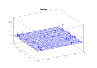
(a) $\beta_{1}<\beta=4.080<\beta_{2}$

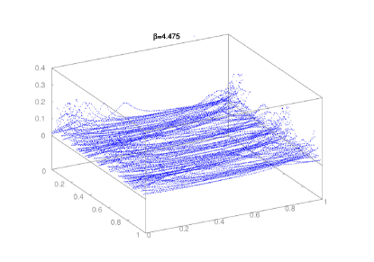
(b) $\beta_{1}<\beta=4.475<\beta_{2}$

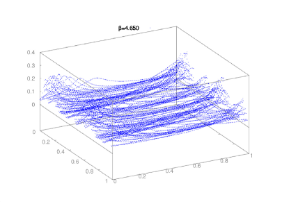
(c) $\beta=4.650>\beta_{2}$

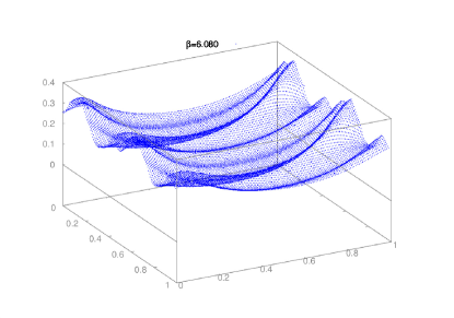
(d) $\beta=6.080>\beta_{2}$

Figure 7.1: The global attractor of the induced polar coordinate system $F_{\beta}$.

As in Section 3, we use polar coordinates in order to study the induced system $F_{\beta}:\mathbb{T}^{1}\times\mathbb{T}^{1}\times[0,\infty)\rightarrow\mathbb{T}^{1}\times\mathbb{T}^{1}\times[0,\infty)$, given by $F_{\beta}(\theta,\alpha,r)=(\gamma\theta,g_{\theta}(\alpha),F_{\beta,\theta,\alpha}(r))$, where $g_{\theta}(\alpha)=\frac{1}{\pi}\arctan\left(\frac{c_{\beta}+d_{\theta}\tan\pi\alpha}{a_{\beta}+b_{\theta}\tan\pi\alpha}\right)\mod 1$, and $F_{\beta,\theta,\alpha}(r)=\frac{\arctan(\beta r)}{3\sqrt{2}}||A(\theta)(\cos\pi\alpha,\sin\pi\alpha)||$

Figures 7.1(a)–7.1(d) illustrate the behaviour of the induced polar coordinate system $F_{\beta}$. Figures 7.1(a) and 7.1(b), show the global attractor shortly after the first critical parameter $(\beta_{1})$ and just before the second $(\beta_{2})$, respectively. Figure 7.1(c) shows $\mathcal{A}_{\beta}(\theta)$ shortly after $\beta_{2}$ where the invariant torus has just formed, and finally, Figure 7.1(d) shows the split off torus far from the bifurcation (all in polar coordinates). For the same values of $\beta$, Figures 7.2(a)–7.2(d) illustrate the behaviour of the global attractor for the original system $f_{\beta}$.

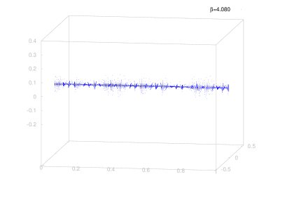
(a) $\beta_{1}<\beta=4.080<\beta_{2}$

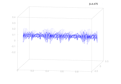
(b) $\beta_{1}<\beta=4.475<\beta_{2}$

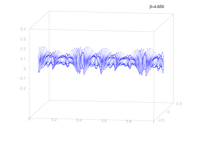
(c) $\beta=4.650>\beta_{2}$

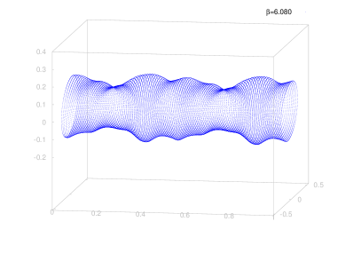
(d) $\beta=6.080>\beta_{2}$

Figure 7.2: The global attractor of the original system $f_{\beta}$.

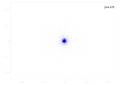
(a) $\beta_{1}<\beta=4.475<\beta_{2}$

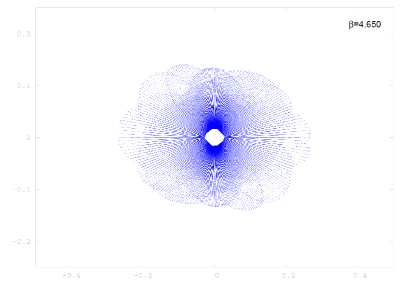
(b) $\beta=4.465>\beta_{2}$

Figure 7.3: 2D projection of the global attractor onto $\mathbb{R}^{2}$

Finally, Figures 7.3(a) and 7.3.(b) show a 2D projection of the torus onto $\mathbb{R}^{2}$ for $\beta=4.475$ (before the torus has formed), and $\beta=4.465$ (after the torus has split off), respectively.

All pictures were produced by using a mixture of pullback and forward iteration for a fixed grid of $(\theta,\alpha)$-coordinates.

References

• [1] C. Grebogi, E. Ott, S. Pelikan, and J.A. Yorke. Strange attractors that are not chaotic. Physica D, 13:261–268, 1984.
• [2] L. Arnold. Random Dynamical Systems. Springer, 1998.
• [3] M.R. Herman Une méthode pour minorer les exposants de Lyapunov et quelques exemples montrant le caractère local d’un théorème d’Arnold et de Moser sur le tore de dimension 2, Comm. Math. Helv. 58:453–502, 1983
• [4] M. Rasmussen. Attractivity and bifurcation for nonautonomous dynamical systems. Number 1907 in Lecture notes in Mathematics. Springer Verlag, 2007.
• [5] C. Pötzsche. Bifurcations in nonautonomous dynamical systems: Results and tools in discrete time. In E. Liz (ed.) et al., Proceedings of the workshop on future directions in difference equations, Vigo, Spain, June 13–17, 2011. Servizo de Publicacións da Universidade de Vigo, Colección Congresos 69, 163-212, 2011.
• [6] M. Rasmussen. Towards a bifurcation theory for nonautonomous difference equations. Journal of Difference Equations and Applications, 12(03-04):297–312, 2006.
• [7] M. Rasmussen. Nonautonomous bifurcation patterns for one-dimensional differential equations. Journal of Differential Equations, 234(1):267–288, 2007.
• [8] H. Zmarrou and A.J. Homburg. Bifurcations of stationary measures of random diffeomorphisms. Ergodic Theory Dyn. Syst., 27(5):1651–1692, 2007.
• [9] H. Zmarrou and A.J. Homburg. Dynamics and bifurcations of random circle diffeomorphisms. Discrete Contin. Dyn. Syst., Ser. B, 10(2–3):719–731, 2008.
• [10] R. Johnson, P. Kloeden, and R. Pavani. Two-step transition in non-autonomous bifurcations: an explanation. Stoch. Dyn., 2(1):67–92, 2002.
• [11] R. Botts, A.J. Homburg, and T. Young. The Hopf bifurcation with bounded noise. Discrete Contin. Dyn. Syst. 32:2997–3007, 2012.
• [12] L. Arnold, E. Oeljeklaus, and E. Pardoux. Almost sure and moment stability for linear Itô equations. In L. Arnold and V. Wihstutz, editors, Lyapunov exponents. Proceedings, Bremen 1984, pages 129–159. Springer-Verlag, Berlin Heidelberg New York, 1986.
• [13] H. Keller and G. Ochs. Numerical approximation of random attractors. In H. Crauel and M. Gundlach, editors, Stochastic dynamics, pages 93–115. Springer, 1999.
• [14] P. Glendinning, T. Jäger, and G. Keller. How chaotic are strange non-chaotic attractors. Nonlinearity, 19(9):2005–2022, 2006.
• [15] K. Bjerklöv. Positive Lyapunov exponent and minimality for a class of one-dimensional quasi-periodic Schrödinger equations. Ergodic Theory Dyn. Syst., 25:1015–1045, 2005.
• [16] J. Stark and R. Sturman. Semi-uniform ergodic theorems and applications to forced systems. Nonlinearity, 13(1):113–143, 2000.
• [17] G. Keller. A note on strange nonchaotic attractors. Fundam. Math., 151(2):139–148, 1996.
• [18] T. Jäger. The creation of strange non-chaotic attractors in non-smooth saddle-node bifurcations. Mem. Am. Math. Soc., 945:1–106, 2009.
• [19] T. Jäger. Quasiperiodically forced interval maps with negative Schwarzian derivative. Nonlinearity, 16(4):1239–1255, 2003.
• [20] V. Anagnostopoulou and T. Jäger. Nonautonomous saddle-node bifurcations: Random and deterministic forcing. J. Diff. Eq., to appear.
• [21] C. Castaing and M. Valadier. Convex Analysis and Measurable Multifunctions. Springer Lecture Notes in Mathematics 580, 1975.
• [22] T. Jäger and G. Keller. A semi-uniform ergodic theorem for random dynamical systems. Preprint 2012, arXiv:1211.5885.
• [23] H. Furstenberg. Strict ergodicity and transformation of the torus. Am. J. Math., 83:573–601, 1961.
• [24] Hans Crauel. Random Probability Measures on Polish Spaces, volume 11 of Stochastics Monographs. Taylor & Francis, 2002.