Synchronization properties of self-sustained mechanical oscillators

Abstract

We study, both analytically and numerically, the dynamics of mechanical oscillators kept in motion by a feedback force, which is generated electronically from a signal produced by the oscillators themselves. This kind of self-sustained systems may become standard in the design of frequency-control devices at microscopic scales. Our analysis is thus focused on their synchronization properties under the action of external forces, and on the joint dynamics of two to many coupled oscillators. Existence and stability of synchronized motion are assessed in terms of the mechanical properties of individual oscillators –namely, their natural frequencies and damping coefficients– and synchronization frequencies are determined. Similarities and differences with synchronization phenomena in other coupled oscillating systems are emphasized.

I Introduction

In electronic devices, time keeping and event synchronization rely upon one or more components able to provide cyclic signals, which are used as frequency references. Since mid-twentieth century, quartz crystals were ubiquitously employed in this function and became standard in the construction of clocks of all kinds. At micrometric scales and below, however, technical difficulties in the fabrication and mounting of quartz crystals motivate considering alternative solutions, preferably based on simpler components. Micromechanical oscillators –tiny vibrating bars of semiconductor material, which can be readily integrated into electronic circuits during manufacturing, and kept in motion by very small electric fields– are an attractive possibility Craighead (2000); Ekinci and Roukes (2005).

In order to function as a frequency reference, an oscillator must perform sustained periodic motion at a frequency determined by its own dynamics (i.e., independent from any external signal). A feedback mechanism able to produce self-sustained motion in a mechanical oscillator Greywall et al. (1994); Yurke et al. (1995) is inspired on the well-known phenomenon of resonance: under the action of external periodic forcing, the response of the oscillator, measured by the amplitude of its motion, is maximal if the external force and the oscillator’s velocity are in-phase or, equivalently, if the oscillator’s displacement from its equilibrium position is a quarter of a cycle late with respect to the force José and Saletan (1998). The feedback self-sustaining mechanism consists in electronically reading the displacement of an autonomous mechanical oscillator, and advancing the signal by a quarter of a cycle, namely, by a positive phase shift $\phi_{0}=\pi/2$ (or, equivalently, a delay of $3\pi/2$). In practice, this shifting in phase can be achieved in a variety of ways –for instance, using resistive circuits or all-pass filters Antonio et al. (2012). The shifted signal is then reinjected as a force acting on the oscillator. To avoid the effect of damping –which would eventually lead the oscillator to rest– the amplitude of the force must be controlled externally and, ultimately, maintained by a battery. Under the action of this conditioned signal, the oscillator moves with maximal amplitude at a frequency determined by its internal parameters (and, possibly, by the amplitude of the self-sustaining feedback force). Figure 1 shows a schematic representation of the self-sustaining circuit.

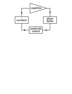
Figure 1: Self-sustained mechanical oscillator. The displacement of the oscillator with respect to its equilibrium position is electronically read, amplified, and shifted in phase. The signal is then reinjected as an amplitude-controlled force acting on the oscillator. Adapted from Ref. 4.

The oscillator’s motion is conveniently described by the Newton equation for a coordinate $x(t)$, representing the displacement from equilibrium:

$$m\ddot{x}+\gamma\dot{x}+kx+\eta(x)=F_{0}\cos(\phi+\phi_{0})+F(t),$$ (1)

where $m$, $\gamma$, and $k$ are effective values for the mass, the damping, and the elastic constant. The term $\eta(x)$ stands for non-elastic forces. The first term in the right-hand side of the equation represents the self-sustaining force. As discussed above, its amplitude $F_{0}$ is an independent parameter, determined by the feedback mechanism. The self-sustaining force depends on the phase of the oscillator’s motion $\phi$, which is defined on the basis that, in harmonic oscillations, $x(t)$ is proportional to $\cos\phi(t)$ (see Sect. II.1). The phase shift between the force and the coordinate should ideally be fixed at $\phi_{0}=\pi/2$ but, in order to assess the effect of this parameter on the oscillator’s dynamics, it is here allowed a generic value. Note that, as a function of $\phi$, the form of the self-sustaining force is not aimed at modeling any specific experimental implementation of the phase shifting, but rather at representing its effect on the reinjected conditioned signal. In addition to $\eta(x)$, the force $F_{0}\cos(\phi+\phi_{0})$ is also a source of nonlinearity: while its phase is directly related to that of $x(t)$, its amplitude is independent of the motion. Finally, $F(t)$ denotes any additional force that may be acting on the oscillator, ranging from externally-applied deterministic signals to electronic noise and thermal fluctuations.

A key technological problem associated with the use of self-sustained mechanical oscillators in micro-devices is the instability of their frequency under the effect of noise Yurke et al. (1995); Ward and Duwel (2011) and of changes in the amplitude of oscillations Agarwal et al. (2007, 2008). Coupling several oscillators to obtain a collective, more robust signal to be used as a frequency reference could be a plausible solution to this problem. It is therefore of much interest to study the synchronization properties of a set of oscillators of this kind interacting with each other.

Our aim in this paper is to characterize the dynamics of self-sustained mechanical oscillators, as governed by Eq. (1). In order to focus on the role of the self-sustaining mechanism, we disregard the nonlinearities represented by the non-elastic forces $\eta(x)$ –although we recognize their importance in the functioning of this kind of oscillators at microscopic scales Antonio et al. (2012). After establishing analytical and numerical procedures to deal with the oscillation phase $\phi$ as a dynamical variable, we first study the properties of self-sustained motion of a single oscillator. Then, taking into account the remark in the previous paragraph, we concentrate on synchronized dynamics in various situations: a self-sustained oscillator under the action of a harmonic external force, two oscillators coupled to each other, and an ensemble of globally coupled oscillators. Our conclusions emphasize similarities and differences with collective motion in other kinds of coupled dynamical systems.

II Dynamics of the self-sustained oscillator

Assuming that non-elastic forces are absent, $\eta(x)\equiv 0$, and redefining the time unit as the inverse of the natural oscillation frequency $\Omega_{0}=\sqrt{k/m}$ and the coordinate unit as $F_{0}/k=F_{0}/m\Omega_{0}^{2}$, Eq. (1) can be recast as two first-order equations for the coordinate $x(t)$ and its velocity $v(t)$,

$$\dot{x} = v,$$

$$\dot{v} = -x-\epsilon v+\cos(\phi+\phi_{0})+f(t),$$ (2)

with $\epsilon=\gamma/m\Omega_{0}$ and $f(t)=F(t)/F_{0}$. Apart from the quantities that determine the self-sustaining and external forces, the only parameter in these equations is the rescaled damping coefficient $\epsilon$. It is worth pointing out that $\epsilon$ coincides with the inverse of the oscillator’s quality (or Q-) factor: $\epsilon=Q^{-1}$. We recall that the quality factor $Q$ is a non-dimensional measure of the resonance bandwidth relative to the resonance frequency, and characterizes the rate of energy dissipation as compared with the oscillation period. In experiments involving micromechanical oscillators Antonio et al. (2012), typical values are around $Q\sim 10^{4}$.

It is important to realize that Eqs. (2) do not specify a dynamical system, for the coordinate and the velocity, in the usual sense. Indeed, as will become clear in the following, the oscillator’s phase $\phi(t)$ cannot be unambiguously defined in terms of $x(t)$ and $v(t)$ alone –although $\phi(t)$ does represent an instantaneous property of the motion. To solve the equations, in any case, an operational definition of the phase becomes necessary. In the next section we discuss how analytical and numerical approaches prompt different ways to deal with this question.

II.1 Analytical treatment and numerical evaluation of the phase

In a typical experiment, even with a high quality factor, a micromechanical oscillator will be found in its long-time asymptotic dynamical regime after at most a few seconds. With $Q=10^{4}$ and a frequency $\Omega=5\times 10^{4}$ Hz Antonio et al. (2012), for instance, any transient regime associated with dissipative effects fades out with a characteristic relaxation time $\tau\sim Q\Omega^{-1}=0.2$ s. If the asymptotic motion is harmonic, to all practical purposes, the oscillation phase is thus well defined when the oscillator’s output signal is fed into the phase shifter to construct the self-sustaining feedback force (see Fig. 1). Tuning the phase shifter allows the experimenter to apply a prescribed shift to the oscillation with no need to measure the phase itself.

On the other hand, both in the analytical and in the numerical treatment of the equations of motion (2), it is necessary to specify the value of the phase at each time, in order to be able to calculate the instantaneous self-sustaining force. The determination of that value must also work during transients or in non-harmonic motion, whose occurrence cannot be discarded a priori when solving the equations.

Analytically, a convenient way to deal with the dependence of the self-sustaining force on the oscillation phase is to introduce $\phi$ itself as one of the variables of the problem. This is achieved by replacing the original coordinate-velocity variables $(x,v)$ by a set of phase-amplitude variables $(\phi,A)$ through a canonical-like transformation José and Saletan (2007),

$$x(t)=A(t)\cos\phi(t),\ \ \ \ \ v(t)=-\nu A(t)\sin\phi(t).$$ (3)

The arbitrary constant $\nu$, which can adopt any real value, parameterizes the variable transformation. As we explain below, it can be chosen in such a way as to make certain solutions of the equations of motion attain a simple mathematical form. The change of variables transforms Eqs. (2) into

$$\dot{A}\cos\phi = A(\dot{\phi}-\nu)\sin\phi,$$

$$\dot{A}\sin\phi = A(\nu^{-1}-\dot{\phi})\cos\phi-\epsilon A\sin\phi$$ (4)

$$-\nu^{-1}\cos(\phi+\phi_{0})-\nu^{-1}f.$$

This formulation has the advantage that the phase is defined for any kind of motion, not only for harmonic oscillations, as $\phi(t)=-\arctan[v(t)/\nu x(t)]$. On the other hand, it turns out to depend on the specific choice of the parameter $\nu$. As a function of the coordinate and the velocity, as advanced above, the oscillator’s phase is therefore not unambiguously defined. Focusing however on harmonic motion –which is characterized by constant amplitude $A$ and constant frequency $\dot{\phi}$– the first of Eqs. (4) makes it clear that the solution will take a particularly simple form if $\nu$ is chosen to coincide with the oscillation frequency. In fact, for $\nu=\dot{\phi}$ and $\dot{A}=0$, that equation is satisfied automatically, and the problem reduces to solve the second equation. In some cases –for instance, in synchronized motion under the action of an external harmonic force (see Sect. II.3)– we know in advance the oscillation frequency, and can therefore conveniently fix $\nu$ before finding the solution. When, on the other hand, the frequency is part of the solution itself –as is the case for an autonomous self-sustained oscillator (Sect. II.2), or for two mutually coupled oscillators (Sect. III.1)– $\nu$ can be considered as an additional unknown of the problem, and obtained together with the solutions to the equations of motion.

In the numerical integration of Newton equations (2), in turn, there are no reasons to assume that the frequency of harmonic solutions is known a priori. Consequently, the phase must be evaluated from the numerical solution itself, as it is progressively obtained, without resorting to a specific change to phase-amplitude variables. The standard method for assigning an instantaneous phase to the signal $x(t)$, through the construction of its analytical imaginary part using the Hilbert transform Benedetto (1996), is here ineffectual, as it requires the whole (past and future) signal to be available at each time where $\phi(t)$ is calculated. We have instead implemented a numerical algorithm that estimates the instantaneous phase in terms of the coordinate along the numerical integration, as follows.

Let $x(t-2h)\equiv x_{1}$, $x(t-h)\equiv x_{2}$ and $x(t)\equiv x_{3}$ be three successive values of the coordinate in the numerical solution with integration step $h$, and define $t_{1}\equiv t-2h$, $t_{2}\equiv t-h$, and $t_{3}\equiv t$. Under the condition discussed below, it is possible to find constants $a$, $w$, and $u$ such that $x_{i}=a\cos(wt_{i}+u)$ for $i=1,2,3$. Obtaining these constants, the phase at time $t$, $\phi(t)=wt_{3}+u$, is given by

$$\cos\phi(t) = \frac{x_{3}}{2x_{2}}\sqrt{\frac{4x_{2}^{2}-(x_{1}+x_{3})^{2}}{x_{2}^{2}-x_{1}x_{3}}},$$

$$\sin\phi(t) = \frac{2x_{2}^{2}-x_{3}(x_{1}+x_{3})}{2x_{2}\sqrt{x_{2}^{2}-x_{1}x_{3}}}.$$ (5)

This solution, however, is well defined only if $|x_{1}+x_{3}|\leq 2|x_{2}|$. It is not difficult to realize that this condition is equivalent to requiring that the three points $x_{1}$, $x_{2}$, and $x_{3}$ define a curve with the same convexity as the fitting cosine function. In the case that $|x_{1}+x_{3}|>2|x_{2}|$, we define three auxiliary points,

$$x^{\prime}_{1}=2\bar{x}-x_{3},\ \ \ x^{\prime}_{2}=2\bar{x}-x_{2},\ \ \ x^{\prime}_{3}=2\bar{x}-x_{1},$$ (6)

with $\bar{x}=(x_{1}+x_{2}+x_{3})/3$, which satisfy $|x^{\prime}_{1}+x^{\prime}_{3}|\leq 2|x^{\prime}_{2}|$ and can therefore be fitted by a cosine. The auxiliary points $x^{\prime}_{i}$ are reflections of the original points $x_{i}$ with respect to the ordinate of their least-square linear fitting, as illustrated in Fig. 2b. Both sets of points, $x^{\prime}_{i}$ and $x_{i}$, have therefore identical linear trends. Consequently, the value of $\phi(t)$ calculated from Eq. (5) using now the auxiliary points, is still a satisfactory evaluation of the phase associated to the points $x_{1}$, $x_{2}$, and $x_{3}$.

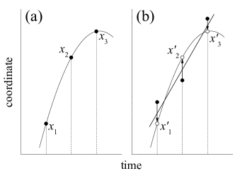
Figure 2: Schematic representation of the numerical evaluation of the oscillation phase. In (a), the coordinates satisfy $|x_{1}+x_{3}|\leq 2|x_{2}|$ and a cosine function exactly fits the three points. In (b), $|x_{1}+x_{3}|>2|x_{2}|$ and the original points (full dots) must be replaced by auxiliary points (primed coordinates, empty dots), obtained by reflection of the original points with respect to the abscissa of their least-square linear fitting (straight line).

Note that our numerical definition of the phase, given by Eqs. (5), is independent of the integration step $h$. In fact, it provides a value for $\phi(t)$ for any trajectory successively passing by the coordinates $x_{1}$, $x_{2}$, and $x_{3}$, with the only condition that they are equally spaced in time. Since in the numerical integration of the equations of motion we need to define the phase at each step, we identify those coordinates with consecutive values of $x(t)$ along the calculation.

Once the phase $\phi(t)$ at a given integration step has been evaluated, it is used to calculate the self-sustaining force $\cos(\phi+\phi_{0})$ and, thus, the numerical increment of the velocity $v(t)$. Since the evaluation of the phase requires knowing the coordinate at three successive steps, in our numerical calculations –which were performed using a second-order Runge-Kutta algorithm– the self-sustaining force was switched on after the first few integration steps had elapsed. This procedure had no significant effect on the subsequent dynamics.

It must be borne in mind that, in general, the analytical definition of $\phi(t)$ using the phase-amplitude variables, and its numerical evaluation in terms of three successive values of the coordinate, are equivalent only when the motion is a harmonic oscillation. Since this kind of motion is not guaranteed a priori, analytical and numerical results must be carefully contrasted with each other when assessing the dynamics of the self-sustained oscillator.

II.2 Self-sustained oscillations

When no external forces act on the oscillator ($f=0$), its motion is controlled by the interplay between its mechanical properties and the self-sustaining force. Assuming that the long-time asymptotic motion is a harmonic oscillation of constant amplitude $A$ and frequency $\dot{\phi}=\Omega$ –which needs not to coincide with the natural frequency $\Omega_{0}\equiv 1$– Eqs. (4) yield

$$A=\frac{\sin\phi_{0}}{\epsilon\Omega},\ \ \ \ \ \Omega=\sqrt{1+\left(\frac{\epsilon}{2\tan\phi_{0}}\right)^{2}}-\frac{\epsilon}{2\tan\phi_{0}}.$$ (7)

These solutions were obtained by fixing $\nu\equiv\Omega$ and separating, in the second of Eqs. (4), terms proportional to $\cos\Omega t$ and $\sin\Omega t$.

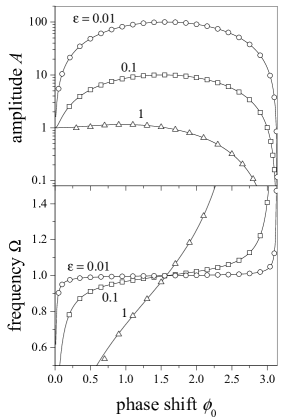
Figure 3: Amplitude and frequency of self-sustained harmonic oscillations as functions of the phase shift of the self-sustaining force, for three values of the damping $\epsilon$. The natural frequency of the oscillator is $\Omega_{0}=1$. Curves: Analytical solution to Eqs. (4), as given by Eqs. (7). Symbols: Numerical solution to Eqs. (2), using the three-point evaluation of the oscillation phase, as described in Sect. II.1.

Figure 3 shows the amplitude and frequency of self-sustained harmonic oscillations as functions of the phase shift $\phi_{0}$ of the self-sustaining force, for three values of the damping $\epsilon$. As advanced in the Introduction, we find that, for small damping (high quality factor), the amplitude is maximal when the phase shift is around $\pi/2$. For $\phi_{0}=\pi/2$, $\Omega$ coincides with the oscillator’s natural frequency, $\Omega_{0}=1$, and the interval where $\Omega\approx\Omega_{0}$ grows as the damping decreases.

Symbols in Fig. 3 represent results obtained from the numerical integration of the Newton equations (2), using the three-point method described in Sect. II.1 for the evaluation of the oscillation phase. In the numerical solutions, the amplitude and the oscillation frequency were measured by recording the coordinate and the time at the integration steps where the velocity changes its sign –from positive to negative, i.e. at the coordinate maxima– and averaging the results over several hundred oscillation cycles after a sufficiently long transient interval. The agreement with the analytical solution is excellent, which validates the assumption of harmonic oscillations.

II.3 Synchronization with harmonic external forcing

Turning the attention to the simplest situation where the synchronization properties of self-sustained oscillators are to be assessed, let us consider a single oscillator subject to the action of an external force with harmonic time dependence, $f(t)=f_{1}\cos\omega t$. As is the case for a broad class of oscillating systems Pikovsky et al. (2003); Manrubia et al. (2004), the self-sustained oscillator is able to synchronize with the external force and perform harmonic motion with frequency $\omega$, provided that $\omega$ and the self-sustained frequency $\Omega$, given by the second of Eqs. (7), are close enough to each other.

Looking for harmonic solutions of frequency $\omega$, Eqs. (4) yield the equation

$$A\left(\omega^{2}-1+{\rm i}\epsilon\omega\right)=-e^{-{\rm i}\phi_{0}}-f_{1}e^{-{\rm i}\psi},$$ (8)

for the amplitude $A$ and phase shift $\psi$ of the coordinate, $x(t)=A\cos(\omega t-\psi)$. Solutions to this equation exist when $\omega$ lies in an interval around $\Omega$, whose width grows with both the damping coefficient $\epsilon$ and the amplitude $f_{1}$ of the external force. For $f_{1}<1$, the interval of existence of synchronized harmonic solutions is determined by the two frequencies

$$\omega_{{}_{2}^{1}}=\frac{\epsilon}{2\alpha_{\pm}}+\sqrt{1+\left(\frac{\epsilon}{2\alpha_{\pm}}\right)^{2}},$$ (9)

with

$$\alpha_{\pm}=\frac{-\sin\phi_{0}\cos\phi_{0}\pm f_{1}\sqrt{1-f_{1}^{2}}}{\cos^{2}\phi_{0}-f_{1}^{2}}.$$ (10)

For $f_{1}\to 0$, both $\omega_{1}$ and $\omega_{2}$ tend to $\Omega$, and the width of the interval of existence vanishes. For $f_{1}<\sin\phi_{0}$, the solution exists if $\omega_{1}\leq\omega\leq\omega_{2}$. For $f_{1}\geq\sin\phi_{0}$, on the other hand, the solution exist for all $\omega\leq\omega_{2}$ if $\phi_{0}<\pi/2$, and for all $\omega\geq\omega_{1}$ if $\phi_{0}>\pi/2$. In the limiting case where $\phi_{0}=\pi/2$, the interval of existence is bounded by

$$\omega_{{}_{2}^{1}}=\sqrt{1+\frac{\epsilon^{2}f_{1}^{2}}{4(1-f_{1}^{2})}}\mp\frac{\epsilon f_{1}}{2\sqrt{1-f_{1}^{2}}}.$$ (11)

Meanwhile, when the amplitude of the external force is larger than that of the self-sustaining force, $f_{1}>1$, synchronized solutions exist for any frequency $\omega$.

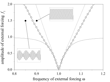
Figure 4: Existence and stability of synchronized motion under the action of an external harmonic force of amplitude $f_{1}$ and frequency $\omega$, for a self-sustaining force with phase shift $\phi_{0}=\pi/2$. The self-sustained frequency is $\Omega=1$, and $\epsilon=0.1$. Dashed lines and empty dots delimitate, respectively, the regions of (analytical) existence and (numerical) stability. Dotted lines correspond to the analytical approximation to the stability region given by Eq. (12). The insets show the coordinate $x(t)$ for two parameter sets (full dots), inside and outside the stability region.

Dashed lines in Fig. 4 delimitate the region in the parameter plane $(\omega,f_{1})$ where synchronized harmonic solutions exist, for a phase shift $\phi_{0}=\pi/2$ and $\epsilon=0.1$, as given by Eq. (11). Numerical integration of Eqs. (2), however, shows that inside this “existence tongue” the motion is not always a harmonic oscillation of frequency $\omega$. In other words, synchronized solutions are actually observed within a subregion of the tongue only, where they are stable. The boundaries of the “stability tongue” are shown by full dots in Fig. 4. They have been found numerically, by dichotomic search of synchronized solutions for selected values of the force amplitude $f_{1}$, until a precision $\delta\omega=5\times 10^{-4}$ was reached in the frequency axis. Motion was considered to be synchronized with the external force when its frequency, calculated from the average period over $10^{3}$ oscillation cycles, differed from $\omega$ by less than $10^{-4}$.

Analytically, the stability of synchronized motion could be determined by means of Floquet theory Bittanti and Colaneri (2010), by linearizing around the time-dependent harmonic solutions. For our two-variable non-autonomous system, however, the theory is not able to provide an explicit condition for stability. An approximate criterion can nevertheless be obtained by replacing all time-periodic terms in the linearized problem by their respective averages. The resulting stability condition is

$$\epsilon+\frac{f_{1}\sin\psi}{\omega A}>0,$$ (12)

where $A$ and $\psi$ are given by Eq. (8). Dotted lines in Fig. 4 show the result of this approximation. While its description of the stability region is not quantitatively good, it correctly reproduces the functional trend with the amplitude of the external force.

The insets in Fig. 4 illustrate the time dependence of the coordinate $x(t)$ inside and outside the synchronization tongue, over a span of $150$ time units. They correspond to an external force of amplitude $f_{1}=1.5$, and frequencies $\omega=0.9$ and $\omega=0.85$, respectively. While, inside the tongue, $x(t)$ maintains a constant oscillation amplitude, the non-synchronized signal displays beats, resulting from a combination of the frequency of the external force and the oscillator’s self-sustained frequency.

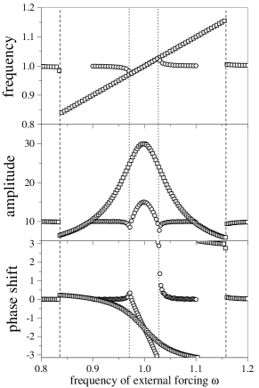
Figure 5: Oscillation frequency, amplitude, and phase shift of an externally forced, self-sustained oscillator ($\Omega=1,\epsilon=0.1$), as functions of the frequency $\omega$ of the external force, for two values of its amplitude, $f_{1}=0.5$ (circles) and $2$ (squares). Dotted and dashed vertical lines indicate the respective boundaries of the synchronization region.

Figure 5 shows numerical results for the oscillation frequency, amplitude, and phase shift for an oscillator of self-sustained frequency $\Omega=1$ ($\phi_{0}=\pi/2$) and $\epsilon=0.1$, as functions of the frequency $\omega$ of the external force, for two values of its amplitude. Circles and squares correspond, respectively, to $f_{1}=0.5$ and $2$. Vertical dotted and dashed lines indicate the respective boundaries of the synchronization region. Results where obtained as explained in Sect. II.2 for Fig. 3, averaging over a large number of oscillation cycles. Outside the synchronization region, where the averages are performed over the beating signal, the average oscillation frequency coincides with $\Omega$ and the amplitude and phase shift have constant values. For the synchronized signal, on the other hand, the frequency equals $\omega$, the amplitude attains a maximum at $\omega=\Omega$, and the phase varies approximately between $\psi=0$ and $\pi$. Note that, at the amplitude maximum, $\psi=\pi/2$. The external force and the self-sustaining force are therefore in-phase at this point, and the amplitude is given by the sum of the values determined by the two forces, $A_{\max}=(1+f_{1})/\epsilon$. Inside the synchronization range, the numerical results for $A$ and $\psi$ are in excellent agreement with the analytical solutions to Eq. (8) which, for clarity, are not shown in the figure.

III Mutual synchronization of self-sustained oscillators

We study now the collective dynamics of a population of mutually coupled self-sustained mechanical oscillators. From the experimental viewpoint, a straightforward way to make the oscillators interact with each other is to substitute the individual self-sustaining force by a linear combination of the feedback signals of all oscillators –built up, for instance, by means of a resistive circuit. To represent this situation, Eqs. (2) are replaced by a set of equations of motion for each oscillator,

$$\dot{x}_{i} = v_{i},$$

$$\mu_{i}\dot{v}_{i} = -\kappa_{i}x_{i}-\epsilon_{i}v_{i}+\sum_{j=1}^{N}f_{ij}\cos(\phi_{j}+\phi_{0j}),$$ (13)

for $i=1,\dots,N$, where $\mu_{i}=m_{i}/m_{0}$, $\kappa_{i}=k_{i}/k_{0}=k_{i}/m_{0}\Omega_{0}^{2}$ are, respectively, the effective mass and elastic constant of oscillator $i$ divided by reference quantities $m_{0}$ and $k_{0}$, used to fix time and coordinate units (see Sect. II). The normalized damping coefficient is $\epsilon_{i}=\gamma_{i}/m_{0}\Omega_{0}$. The coefficient $f_{ij}$ weights the contribution of the self-sustaining force of oscillator $j$ to the coupling signal applied to oscillator $i$, and $\phi_{0j}$ is the corresponding phase shift. The size of the population is $N$.

The profusion of free coefficients in Eqs. (13) calls for some simplifying assumptions, both on the diversity of individual dynamical parameters and on the coupling force. In the following sections, therefore, we focus on the special situation where all self-sustaining forces have the same weight in the interaction, and all oscillators are feeded the same coupling force: $f_{ij}=N^{-1}$ for all $i$, $j$. The dependence of these coefficients on the number of oscillators $N$ warrants that the coupling force is comparable between populations of different sizes. Moreover, we assume that the phase shift is the same for all oscillators, $\phi_{0i}=\phi_{0}$ for all $i$, and usually consider the maximal-response value $\phi_{0}=\pi/2$. The parameters $\mu_{i}$, $\kappa_{i}$, and $\epsilon_{i}$ are, in principle, left to vary freely. In our numerical simulations, however, we fix $\kappa_{i}=1$ for all $i$, choosing to control the diversity of the individual natural frequencies, $\Omega_{i}=\sqrt{\kappa_{i}/\mu_{i}}$, by means of the mass ratios $\mu_{i}$ only.

III.1 Two-oscillator synchronization

The joint dynamics of two coupled oscillators serves as an illustrative intermediate case between a single oscillator subject to external forcing and an ensemble of interacting oscillators. We take the parameters of oscillator $1$ as reference values for defining time and coordinate units, so that $\mu_{1}=\kappa_{1}=1$. Its natural frequency is, therefore, $\Omega_{1}=1$.

In synchronized motion, the two oscillators are expected to perform harmonic oscillations with a common frequency $\Omega_{s}$ and a certain phase shift between each other: $x_{1}(t)=A_{1}\cos(\Omega_{s}t-\psi)$, $x_{2}(t)=A_{2}\cos\Omega_{s}t$. Using this Ansatz in the phase-amplitude representation, we get the equations

$$A_{1}\left(\Omega_{s}^{2}-1+{\rm i}\epsilon_{1}\Omega_{s}\right) = -e^{-{\rm i}\phi_{0}}\frac{1+e^{-{\rm i}\psi}}{2},$$

$$A_{2}\left(\mu_{2}\Omega_{s}^{2}-\kappa_{2}+{\rm i}\epsilon_{2}\Omega_{s}\right) = -e^{-{\rm i}\phi_{0}}\frac{1+e^{{\rm i}\psi}}{2},$$ (14)

to be solved for $\Omega_{s}$, $A_{1}$, $A_{2}$, and $\psi$. Compare these equations with Eq. (8).

Solutions to Eqs. (14) exist for arbitrary values of all the involved parameters. Numerical resolution of the respective Newton equations, however, reveals that synchronization is observed only when the self-sustained frequencies of the two oscillators are sufficiently close to each other. Otherwise, synchronized motion is unstable. The synchronization range turns out to depend on the damping coefficients $\epsilon_{i}$, becoming wider as the damping increases. Full dots in Fig. 6 show the boundary of the stability tongue for the case $\epsilon_{1}=\epsilon_{2}$, in the plane whose coordinates are the ratio of the oscillators’ natural frequencies, $\Omega_{2}/\Omega_{1}$ (which, for $\phi_{0}=\pi/2$, coincide with the self-sustained frequencies), and the damping coefficient $\epsilon_{2}$. Empty symbols correspond to the case where $\epsilon_{1}$ is fixed and $\epsilon_{2}$ varies. Results for $\epsilon_{1}=10^{-3}$, not shown in the plot, are practically coincident with those for $\epsilon_{1}=0.01$, which thus constitute a good representation of the limit of very small $\epsilon_{1}$. For $\epsilon_{1}=0.1$, on the other hand, the tongue has an appreciable size even for very small $\epsilon_{2}$, indicating that the width of the synchronization range is controlled by the larger damping coefficient.

Figure 6: Stability regions for synchronized motion of two coupled oscillators with natural frequencies $\Omega_{1}=1$ and $\Omega_{2}$ ($\phi_{0}=\pi/2$). Empty and full symbols correspond, respectively, to the case of fixed damping coefficient for oscillator $1$, and to equal damping for both oscillators.

For $\phi_{0}=\pi/2$, the solution to Eqs. (14) for the synchronization frequency is

$$\Omega_{s}=\sqrt{\frac{\kappa_{2}+\epsilon_{2}/\epsilon_{1}}{\mu_{2}+\epsilon_{2}/\epsilon_{1}}}.$$ (15)

Note that $\Omega_{s}$ always lies in the interval between $\Omega_{1}=1$ and $\Omega_{2}=\sqrt{\kappa_{2}/\mu_{2}}$ –either for $\Omega_{1}<\Omega_{2}$ or vice versa. For $\epsilon_{2}\ll\epsilon_{1}$ we have $\Omega_{s}\approx\Omega_{2}$, while for $\epsilon_{2}\gg\epsilon_{1}$ we have $\Omega_{s}\approx\Omega_{1}$. Therefore, the common frequency of the synchronized oscillators approaches the natural frequency of the oscillator with the smaller damping coefficient. The oscillator with the larger quality factor thus drives synchronized motion.

The upper panel in Fig. 7 shows, as symbols, the numerical evaluation of the oscillation frequencies of two coupled self-sustained oscillators with $\phi_{0}=\pi/2$ and $\epsilon_{1}=\epsilon_{2}=0.1$, as functions of the ratio of their natural frequencies, $\Omega_{2}/\Omega_{1}$. They have been calculated from the numerical solution to Newton equations, as explained in previous sections. Much as in the case of a single oscillator subject to an external force (see upper panel of Fig. 5), the frequencies change abruptly as the boundary of the synchronization range is traversed. The curve stands for the analytical prediction for the synchronization frequency, given by Eq. (15).

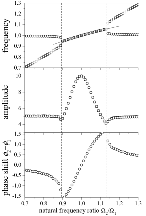
Figure 7: Oscillation frequency (upper panel), amplitude (central panel), and phase shift (lower panel) of two coupled self-sustained oscillators with $\epsilon_{1}=\epsilon_{2}=0.1$ and $\phi_{0}=\pi/2$, as functions of the natural frequency ratio $\Omega_{2}/\Omega_{1}$. Vertical dashed lines indicate the boundaries of the synchronization range. In the two uppermost panels, circles and squares correspond to oscillators $1$ and $2$, respectively. The curve in the upper panel represents the analytical result for the synchronization frequency.

The central and lower panels in Fig. 7 display numerical results for the oscillation amplitude and phase shift between the two oscillators. Since, except for their natural frequencies, the two oscillators are identical and the coupling force acting over them is the same, their amplitudes are only slightly different outside the synchronization range and are exactly coincident inside. For $\Omega_{2}=\Omega_{1}$ the amplitudes reach their maximum, $A_{\max}=\epsilon^{-1}$. At that point, the two oscillators are in-phase, $\phi_{2}-\phi_{1}=\psi=0$, and their respective contributions to the coupling force have always the same sign and magnitude. At the boundaries of the synchronization range, on the other hand, the phase shift attains values around $\pm\pi/2$. Note, finally, that for $\Omega_{2}<\Omega_{1}$ and $\Omega_{2}>\Omega_{1}$ we have, respectively, $\phi_{2}-\phi_{1}<0$ and $\phi_{2}-\phi_{1}>0$. Thus, irrespectively of whether they are synchronized or not, the oscillator with the lower natural frequency is always retarded with respect to its partner.

III.2 Collective synchronization of oscillator ensembles

The results obtained in the previous sections suggest that, in a population of coupled self-sustained oscillators, synchronized motion would be observed if their individual natural frequencies, $\Omega_{i}=\sqrt{\kappa_{i}/\mu_{i}}$, are sufficiently close to each other. It is under this condition that oscillators could become mutually entrained, so as to perform coherent collective dynamics. The dispersion of natural frequencies should therefore control the capability of the ensemble to display synchronization. In a large population, in any case, the tendency to entrainment of oscillators with similar frequencies is expected to compete with the disrupting effect of non-synchronized oscillators, whose incoherent signal influences the whole system through the coupling force. We show in this section that this competition gives rise to complex collective behavior, including partial synchronization in the form clustering.

The only kind of collective motion that can be dealt with with our analytical tools corresponds to the case of full synchronization of the whole ensemble, where all oscillators move with the same frequency $\Omega_{s}$, but are generally out-of-phase with respect to each other. Writing the coordinate of each oscillator as $x_{i}(t)=A_{i}\cos(\Omega_{s}t-\psi_{i})$, the phase-amplitude representation of Newton equations (13) yields

$$A_{i}(\mu_{i}\Omega_{s}^{2}-\kappa_{i}+{\rm i}\epsilon_{i}\Omega_{s})e^{{\rm i}\psi_{i}}=-\frac{e^{-{\rm i}\phi_{0}}}{N}\sum_{j=0}^{N}e^{{\rm i}\psi_{j}},$$ (16)

for $i=1,\dots,N$. The complex factor $z=N^{-1}\sum_{j}\exp({\rm i}\psi_{j})$ in the right-hand side provides a collective characterization of the distribution of relative phases in the oscillator ensemble. Note that its modulus $\rho=|z|$ coincides with the order parameter used in Kuramoto’s theory for phase oscillator synchronization to quantitatively assess the synchronization transition Kuramoto (2003); Manrubia et al. (2004). When phases are homogeneously distributed over $(0,2\pi)$, we have $\rho\sim N^{-1/2}$, and $\rho$ grows approaching unity as phases accumulate toward each other.

Equations (16) make it possible to show that, for $\phi_{0}=\pi/2$, the synchronization frequency $\Omega_{s}$ and the order parameter $\rho$ satisfy

$$0 = \sum_{i=1}^{N}\frac{\mu_{i}\Omega_{s}^{2}-\kappa_{i}}{\sqrt{(\mu_{i}\Omega_{s}^{2}-\kappa_{i})^{2}+\epsilon_{i}^{2}\Omega_{s}^{2}}},$$

$$\rho = \sum_{i=1}^{N}\frac{\epsilon_{i}\Omega_{s}}{N\sqrt{(\mu_{i}\Omega_{s}^{2}-\kappa_{i})^{2}+\epsilon_{i}^{2}\Omega_{s}^{2}}}.$$ (17)

Figure 8 and its inset represent, as curves, the order parameter and the synchronization frequency obtained from these equations for an ensemble where natural frequencies are drawn from a Gaussian distribution with mean value $\bar{\Omega}=1$ and mean square dispersion $\sigma$, in the limit $N\to\infty$. We have taken $\kappa_{i}=1$ for all $i$, so that each natural frequency fixes univocally the mass ratio $\mu_{i}$. The damping coefficients are equal for all oscillators, $\epsilon_{i}=0.1$ for all $i$. When the frequency dispersion is small we have $\rho\approx 1$, indicating that the phase shift between oscillators in the synchronized state is small as well. As $\sigma$ grows, $\rho$ decreases monotonically, and phases become less similar to each other. The inset, in turn, shows that the synchronization frequency changes only slightly from $\bar{\Omega}$, decreasing by less that 1% over two orders of magnitude of variation in $\sigma$.

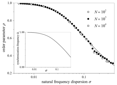
Figure 8: The order parameter $\rho$ as a function of the mean square dispersion of natural frequencies, for an ensemble of size $N$. Natural frequencies are extracted from a Gaussian distribution with mean value $\bar{\Omega}=1$. All oscillators have damping coefficient $\epsilon_{i}=0.1$. Dots stand for numerical results for three values of $N$, and the curve is the analytical result for $N\to\infty$, obtained from Eqs. (17) in the continuous limit. The corresponding result for the synchronization frequency $\Omega_{s}$ is shown in the inset.

Symbols in the main plot of Fig. 8 correspond to the evaluation of the order parameter from the numerical solution of Newton equations for three population sizes, with natural frequencies drawn at random from the same distribution as above. For dispersions below $\sigma\approx 0.13$, the numerical results for different sizes are in excellent agreement between themselves and with the analytical prediction. For $\sigma\gtrsim 0.13$, on the other hand, numerical and analytical results depart from each other. Inspection of the ensemble for those values of $\sigma$ shows that oscillators are in fact not synchronized. Not all of them oscillate with the same frequency and, consequently, the coherent motion of phases breaks down. This explains that the order parameter calculated from the numerical solution of the equations of motion lies generally below the analytical prediction, which assumes full synchronization of the ensemble.

Numerical results show that, when full synchronization is not observed, a part of the ensemble splits into several internally synchronized clusters. The oscillation frequency of the members of each cluster –determined, as in previous sections, from the average period between successive maxima in their coordinates– is the same, while the frequency differs between clusters. This state of partial synchronization is reminiscent of the clustering regime of coupled chaotic elements, which has been profusely reported for both continuous-time dynamical systems for maps Manrubia et al. (2004); Kaneko (1990, 1994); Zanette and Mikhailov (1998a, b, 2000). In our case, clustering seems to be induced by stochastic fluctuations in the distribution of natural frequencies: clusters tend to form where the randomly chosen frequencies become accumulated by chance. Clustering in ensembles of coupled dynamical elements is a highly degenerate regime, where the collective state of the system strongly depends on the specific choice of the individual parameters –in the present situation, the natural frequencies– and initial conditions. Necessarily, therefore, the study of this regime is restricted to numerical analysis, and to a semi-quantitative illustration of its main features. While the results presented below pertain to a specific realization of the oscillator ensemble, they are demonstrative of the generic behavior within the clustering regime.

We consider an ensemble of $N=100$ coupled oscillators, all with the same damping coefficient $\epsilon_{i}=0.1$. In order to be able to do a detailed comparison of individual dynamics for different values of the mean square dispersion of natural frequencies, each natural frequency is defined as a function of $\sigma$, given by $\Omega_{i}(\sigma)=\bar{\Omega}+\sigma r_{i}$. Here, $r_{i}$ is a random number extracted from a Gaussian distribution of zero mean and unitary variance, chosen once for each oscillator and all values of $\sigma$. In this way, individual natural frequencies maintain their relative difference with $\bar{\Omega}$ as $\sigma$ varies. We take, as above, $\bar{\Omega}=1$.

The upper panel of Fig. 9 shows the oscillation frequency of individual oscillators, calculated from the average interval between their coordinate’s maxima, as a function of the natural frequency dispersion $\sigma$. Each curve corresponds to an oscillator; heavier curves (green/light grey and red/dark grey) stand for the frequencies of two oscillators whose individual dynamics are analyzed in more detail below. Oscillation frequencies have been evaluated at $2000$ values of $\sigma$ within the limits of the plot, and then interpolated by means of spline functions in order to smooth out some sharp fluctuations, especially in the large-$\sigma$ range.

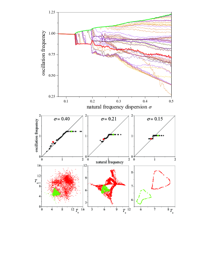
Figure 9: (Color online) Upper panel: Individual oscillation frequencies in an ensemble of $N=100$ oscillators, as functions of the mean square dispersion of natural frequencies $\sigma$. The two heavier lines (green/light grey and red/dark grey) correspond to two oscillators selected for more detailed analysis (see text). Middle panels: Oscillation frequencies as functions of natural frequencies for all oscillators in the ensemble, and three values of $\sigma$. The two selected oscillators are marked with their respective colors/shades. Lower panels: Recurrence plots for the time intervals $T_{n}$ between maxima in the coordinates of the two selected oscillators, for the same values of $\sigma$ as in the middle panels.

The plot shows how, as the dispersion $\sigma$ decreases, increasingly many oscillators aggregate into clusters. Close inspection of individual curves reveals the considerable complexity of the process. While many oscillators join their nearest clusters, others perform substantial frequency excursions before becoming integrated into a cluster –see, for instance, the oscillator with the lowest oscillation frequency for $\sigma=0.5$. Some small groups of oscillators with neighboring frequencies seemingly coalesce into well defined clusters, only to become dispersed as $\sigma$ decreases further, probably due to the disrupting effect of larger and more coherent groups. Once the ensemble is split into just a few clusters, their mutual collapse occurs within narrow intervals of the dispersion, as seen to happen for $\sigma\approx 0.2$. For $0.13\lesssim\sigma\lesssim 0.2$, in turn, the migration of a few oscillators from one cluster to another is especially noticeable, though this phenomenon is also observed in other zones of the plot. The final collapse into a single cluster takes place at $\sigma\approx 0.13$, where –as we have found above, from the results displayed in Fig. 8– the order parameter attains the theoretical value corresponding to full synchronization.

The development of clusters is apparent in the plots of the middle panels of Fig. 9, where individual oscillation frequencies are plotted versus the respective natural frequencies for three selected values of the dispersion of natural frequencies. In this kind of plot, where each dot represents a single oscillator, plateaus of constant oscillation frequencies stand for clusters formed by mutually synchronized oscillators. On the other hand, dots near the diagonal correspond to oscillators which remain almost immune to the collective force exerted by the ensemble. For $\sigma=0.40$ (left panel), most of the population is unsynchronized, although a well developed cluster is already present at large frequencies. This cluster contains $28$ of the $100$ oscillators, whose oscillation frequencies differ by about one part in $10^{4}$. There are, however, at least three more groups with similarly close frequencies, but none of them contains more than four oscillators. For $\sigma=0.21$ (central panel), the large-frequency cluster has grown to encompass $42$ oscillators, while a cluster with $13$ oscillators has appeared at intermediate frequencies. A few smaller groups, of about five synchronized oscillators each, are also present. For $\sigma=0.15$ (right panel), all but three oscillators are distributed among two clusters. Of these three oscillators –which, as we can see from the upper panel, are migrating between the clusters as $\sigma$ varies– two are mutually synchronized, with oscillation frequencies differing by one part in $10^{5}$. The large, low and high-frequency clusters contain $32$ and $65$ oscillators, respectively.

Finally, in order to have a glance at the dynamics of individual oscillators, we have constructed recurrence plots for the time intervals $T_{n}$ between successive maxima in their coordinates –the same intervals used to numerically evaluate the oscillation frequencies. We have selected two oscillators, which we denote by A and B, with natural frequencies at both sides of the mean value $\bar{\Omega}=1$: $\Omega_{\rm A}\approx 1.17$ and $\Omega_{\rm B}\approx 0.83$. In the plots of Fig. 9, they are represented by two colors/shades: green/light grey and red/dark grey, respectively.

The lower panels in Fig. 9 display, for both oscillators, the recurrence plots $T_{n+1}$ vs. $T_{n}$ along a few thousand successive values of $n$ and for the same values of $\sigma$ as in the middle panels. Note that, in this kind of plot, harmonic motion would be represented by a single fixed point. For $\sigma=0.40$, the irregular distribution of dots –with just a weak hint at an underlying structure, given by the partially overlapping clouds– suggests the occurrence of high-dimensional chaotic dynamics. We point out that chaotic motion on a high-dimensional attractor is the generic behavior expected for the ensemble when oscillations are not fully synchronized. Our dynamical system, in fact, is dissipative and nonlinear, and evolves in a phase space of many dimensions. Clearly, this irregular motion is driven by the complicated time-dependence of the coupling force, which integrates the contributions coming from the mutually incoherent evolution of most oscillators. Remarkably, while this force is the same for all oscillators, the recurrence plot for $\sigma=0.40$ shows that its effect on their individual dynamics can be quantitatively different. Oscillator A, which already belongs to a large synchronized cluster (see middle panels of Fig. 9), is restricted to a relatively small zone of the plot, fluctuating between $T_{n}\approx 4$ and $8$. Oscillator B, on the other hand, is not synchronized for this value of $\sigma$, and the corresponding time intervals broadly vary between $T_{n}\approx 2$ and $14$.

Oscillators A and B remain, respectively, synchronized and unsynchronized for $\sigma=0.21$. The distribution of dots in the recurrence plot is still irregular, but has become considerably more structured than for higher $\sigma$. For oscillator B, in particular, the picture is reminiscent of the attractor of a low-dimensional chaotic map. This hints at a considerable decrease in the effective dimensionality of our system, as the organization of the ensemble into synchronized clusters progresses.

For $\sigma=0.15$, the situation is qualitatively different. As discussed above, practically all the ensemble is now divided into just two synchronized clusters, comprising about one and two thirds of the whole population. The coupling force is thus expected to consist of essentially two components, each of them with the frequency of one of the clusters. Accordingly, the distribution of dots in the corresponding recurrence plot over well-defined closed curves suggests quasiperiodic motion. Moreover, they are bounded to a much smaller region of the plane, with variations in $T_{n}$ of around one time unit. The collective organization in this partially synchronized state has therefore led to a drastic decrease in the dynamical complexity, with a large reduction in the dimensionality of individual motion and a strong limitation to its deviation from harmonic oscillations.

It should be clear that the above quantitative details about the clustering dynamics of the oscillator ensemble –such as the number of clusters at each value of $\sigma$, the number of oscillators in each cluster, or the values of $\sigma$ at which the major cluster collapses take place– are specific to the ensemble obtained from a particular realization of the random numbers $r_{i}$, which define the individual natural frequencies. However, the generic picture arising from the study of this particular case illustrates the features typically expected for our system in the clustering regime.

IV Discussion and conclusion

In this paper, we have studied the synchronization dynamics of a linear mechanical oscillator whose motion is sustained by a feedback force, constructed through the conditioning of a signal produced by the oscillator itself. This self-sustaining force –which, in an experimental setup, can be generated electronically– is an amplitude-controlled, phase-shifted copy of the oscillator’s displacement from equilibrium. If the phase shift is appropriately chosen, namely, if the force and the oscillator’s velocity are in-phase, the response of the system is optimized and the oscillations attain maximal amplitude. Under the action of the self-sustaining force, and for asymptotically long times, the oscillator performs harmonic motion with a frequency determined by the interplay between its mechanical parameters (mass, elastic constant, damping coefficient) and those of the force itself.

Besides their plausible usefulness in the design of micromechanical devices, on which we commented in the Introduction, oscillators of this kind constitute an interesting class of non-standard mechanical systems. In fact, the variables in their equation of motion are not just the coordinate and the velocity, but also the oscillation phase, whose instantaneous value cannot be unambiguously defined in terms of the former. The dynamical properties of these oscillators –in particular, those related to synchronized motion, which are relevant to potential applications– are therefore worth analyzing.

As a first step, we have considered the effect of an external harmonic force on a single self-sustained oscillator. It is well known that an ordinary linear mechanical oscillator responds to harmonic forcing by asymptotically oscillating at exactly the same frequency as the force, irrespectively of the difference with its natural frequency. Our self-sustained oscillator, on the other hand, synchronizes to the external force only if the difference between the two frequencies is below a certain threshold. This synchronization range grows as the oscillator’s damping coefficient and the amplitude of the external force increase. In this sense, the self-sustained oscillator belongs to the wider class of oscillating systems which can be entrained by external forces only if the natural frequency and the forcing frequency are not too dissimilar. However, in contrast to simpler systems –for instance, Kuramoto’s phase oscillators Kuramoto (2003); Manrubia et al. (2004)– the frequency range where synchronized dynamics is a solution to the equations of motion does not coincide with the range where the same solution is stable. Specifically, the existence range is always wider than the stability range. When the amplitude of the external force is larger than that of the self-sustaining force, in particular, synchronized solutions exist for any frequency difference, while they are stable for sufficiently small differences only.

We analyzed mutual synchronization of coupled oscillators, first, in the case of two oscillators whose individual self-sustaining forces were replaced by a common feedback force. This coupling signal consisted of a linear combination of the two self-sustaining forces, with equal weights for both contributions. The respective phase shifts were also identical. Under these conditions, synchronized solutions exist for arbitrary values of the oscillators’ self-sustained frequencies. The two synchronized oscillators perform harmonic motion with a common frequency, whose value lies between the two self-sustained frequencies. As in the case of synchronization with an external force, however, synchronized motion is not always stable. Mutual entrainment requires that the self-sustained frequencies are sufficiently close to each other and, again, the synchronization range grows with the oscillator’s damping coefficients. The requirement of small frequency differences to ensure synchronization was stated several years ago for other coupled systems whose individual dynamics exhibit, as in our case, limit-cycle oscillations Aronson et al. (1990); Matthews and Strogatz (1990); Reddy et al. (1998). It is however interesting to point out that, in those systems, the synchronization range is flanked, for sufficiently intense coupling, by a regime of “oscillation death.” In this regime, due to the effect of coupling, the unstable fixed points inside individual limit cycles become stable through an inverse Hopf bifurcation, and all trajectories are asymptotically attracted toward them. The long-time joint evolution is therefore trivial. In contrast, our self-sustained oscillators do not possess fixed points in their individual dynamics, and oscillation death is not observed.

For ensembles formed by many oscillators, the common coupling force was constructed by combining equally weighted contributions from all the elements. Coupling was therefore homogeneous and global over the ensemble. Being a function of the individual oscillation phases, the coupling force is straightforwardly related to Kuramoto’s order parameter for synchronization in populations of phase oscillators Kuramoto (2003). This same order parameter can thus be used to quantify the degree of coherence in our system. Assuming that the ensemble is fully synchronized, with all oscillators moving with the same frequency but shifted in phase from each other, it is possible to show that the order parameter decreases as the dispersion in the self-sustained frequencies over the ensemble grows, which reveals an increasing dispersion in their relative phase shifts. In contrast with the case of Kuramoto’s phase oscillators, however, the order parameter does not vanish for any finite value of the frequency dispersion. This suggests that a synchronization transition similar to that occurring in ensembles of phase oscillators is absent in our system. Numerical resolution of the equations of motion, however, shows that the state of full synchronization is not observed when the frequency dispersion is large. Instead, the ensemble splits into several groups of mutually synchronized oscillators, whose number and size vary with the frequency dispersion, and with further decrease of the order parameter. This is a typical regime of clustering, reminiscent of the behavior of coupled chaotic dynamical systems just below the synchronization transition Manrubia et al. (2004), or of ensembles of coupled oscillators with highly heterogeneous frequency distribution Mikhailov et al. (2004). In our system, this highly degenerate collective state seems to be triggered by fluctuations in the distribution of frequencies, with clusters forming where frequencies accumulate randomly. The ensemble of interacting self-sustained oscillators, in any case, shares with other coupled systems the characteristic dynamical complexity of the clustering regime.

In order to focus on the effect of the self-sustaining mechanism, we have disregarded any other non-linear contribution to the individual dynamics of the oscillators. Non-elastic forces, however, play a key role in the functioning of self-sustained oscillators at microscopic scales. As we have discussed in the Introduction, such forces are responsible for the amplitude dependence of the oscillation frequency –an undesired effect in frequency-control devices Agarwal et al. (2007, 2008); Antonio et al. (2012). Hence, the next step in the study of this kind of mechanical systems is to analyze the interplay between self-sustaining and other non-linear forces, characterizing their joint influence on synchronized motion. This is the subject of work in progress.