LOW SENSITIVITY OPTION FOR TRANSVERSE OPTICS OF THE FLASH LINAC AT DESY

Abstract

The aim of the FLASH linac is to create electron bunches of small transverse emittance and high current for the free-electron laser facility FLASH at DESY. Available operational experience indicates that in order to optimize SASE signal at different wavelengths or to fine-tune the FEL wavelength, empirical adjustment of the machine parameters is required and, therefore, the sensitivity of the beamline to small changes in the beam energy and in the magnet settings becomes one of the important issues which affects both, the final performance and the reproducibility of the results after breaks in operation. In this article the transverse optics of the FLASH beamline with low sensitivity to changes in beam energy and quadrupole settings is presented. This optics is in operation since spring 2006 and has shown a superior performance with respect to the previous setup of the transverse focusing.

1 ACCELERATOR OVERVIEW

The free-electron laser FLASH at DESY, based on self-amplified spontaneous emission (SASE), is the unique user facility operating in the VUV and the soft X-ray wavelength range. Since summer 2005, it provides coherent femtosecond long radiation to user experiments [1, 2]. Fig. 1 shows the current layout of the facility. Electron bunches are produced in an RF gun and accelerated in six cryomodules (ACC1 - ACC6) each containing eight nine-cell superconducting cavities of the TESLA type and a doublet of superconducting quadrupoles. To achieve high peak current in the undulator, the bunch is longitudinally compressed in two magnetic chicanes. Downstream the first bunch compressor BC2 (a four bend chicane) there is a diagnostic section (DBC2) equipped with several OTR screens for the measurement of beam profiles. A second compression stage takes place after the passage through ACC2 and ACC3 and is performed using a S-type chicane (BC3). The last accelerating section, presently containing three cryomodules (ACC4, ACC5 and ACC6), accelerates the beam to the chosen final energy (presently up to 1 GeV). Then, the electron beam is either guided to a bypass beam line (not shown in Fig. 1) or brought through a collimator section to the undulator. The collimator section has a dogleg shape and contains transverse and energy collimators for undulator protection purposes. Finally, the electron beams from the undulator and bypass are dumped in the same absorber (DUMP).

Figure 1: Current layout of the FLASH facility (top view). Beam direction is from left to right. Blue, green, and orange colors mark dipole and quadrupole magnets, and undulator segments, respectively. Yellow color indicates gun cavity, accelerating cavities and transverse-deflecting cavity.

2 TWISS PARAMETERS FOR ACCELERATED BEAM

We will assume that the transverse particle motion is uncoupled in linear approximation and will use the variables $x_{\delta}$ and $q_{\delta}$ for the description of the horizontal beam oscillations. Here, as usual, $x_{\delta}$ is the horizontal particle coordinate and $q_{\delta}$ is the horizontal canonical momentum scaled with the kinetic momentum of the reference particle $p_{\delta}$, and the exact meaning of the subscript $\delta$ will be clarified in the following sections.

If the beam undergoes acceleration, $p_{\delta}$ is not constant along the accelerator and in this case there are different methods of including the beam energy variation in the lattice functions which could lead, for example, to lattice functions that, for a given periodic structure, decrease with increasing beam energy. We will use as definition of the Twiss parameters the second order moments of the beam distribution, namely

$$\beta_{\delta}=\frac{\left<x_{\delta}^{2}\right>}{\epsilon_{x}^{\delta}},\;\;\;\;\alpha_{\delta}=-\frac{\left<x_{\delta}q_{\delta}\right>}{\epsilon_{x}^{\delta}},\;\;\;\;\gamma_{\delta}=\frac{\left<q_{\delta}^{2}\right>}{\epsilon_{x}^{\delta}},$$ (1)

where

$$\epsilon_{x}^{\delta}=\sqrt{\left<x_{\delta}^{2}\right>\left<q_{\delta}^{2}\right>-\left<x_{\delta}q_{\delta}\right>^{2}}$$ (2)

is the rms emittance. With this definition, the Twiss matrix

$$B_{\delta}=\left(\begin{array}[]{rr}\beta_{\delta}&-\alpha_{\delta}\\ -\alpha_{\delta}&\gamma_{\delta}\end{array}\right)$$ (5)

satisfies the equation

$$\frac{dB_{\delta}}{d\tau}=JH_{\delta}B_{\delta}-B_{\delta}H_{\delta}J,$$ (6)

where $\tau$ is path length along the accelerator, matrix $J$ is the symplectic unit and the matrix $H_{\delta}$ is always symmetric (see equation (23) below).

The solution of (6) is given by the formula

$$B_{\delta}(\tau)=M_{\delta}(\tau)\,B_{\delta}(0)\,M_{\delta}^{\top}(\tau),$$ (7)

where the matrix $M_{\delta}$ satisfies the equation

$$\frac{dM_{\delta}}{d\tau}=JH_{\delta}M_{\delta}\,,\;\;M_{\delta}(0)=I\,,$$ (8)

and is symplectic.

Alternatively, the matrix $M_{\delta}$ can be expressed using Twiss parameters, if they are known, in the familiar form

$$M_{\delta}(\tau)=T_{\delta}^{-1}(\tau)\,R(\mu_{\delta}(\tau))\,T_{\delta}(0).$$ (9)

Here $R(\mu_{\delta})$ is a 2 by 2 rotation matrix, $\mu_{\delta}$ is the horizontal phase advance (defined as usual using the integral of the reciprocal of the betatron function) and

$$T_{\delta}=\left(\begin{array}[]{cc}1/\sqrt{\beta_{\delta}}&0\\ \alpha_{\delta}/\sqrt{\beta_{\delta}}&\sqrt{\beta_{\delta}}\end{array}\right).$$ (12)

Note that, if we assume that the dynamics in the variables $x_{\delta}$ and $q_{\delta}$ is given by the matrix $A_{\delta}$, then the following identity holds

$$M_{\delta}(\tau)=\frac{1}{\sqrt{\det\left(A_{\delta}(\tau)\right)}}\cdot A_{\delta}(\tau)\,.$$ (13)

3 OPTICS OPTION I

The beam line discussed in this paper starts from the quadrupole doublet of the ACC1 cryomodule and ends at the entrance of the SASE undulator. We consider neither the beam dynamics in the gun area nor the choice for the setting of the undulator quadrupoles (important topic, which deserves separate consideration).

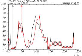
Figure 2: Optics Option I. The SASE undulator starts at the position $s\approx 190m$.

Optics option I, which was prepared for the commissioning is described in [3] and is shown in Fig. 2. It may look somewhat non-typical for the straight beam line with its two bulges, but it was the only way to satisfy certain lattice constraints, which were considered at that time as important. These constraints include among others

A special choice of Twiss parameters in the bunch compressors BC2 and BC3 reduces the emittance growth due to coherent synchrotron radiation (CSR).

The selection of the optical functions in the collimator section is determined by the need to suppress the dispersion and to shape the beam envelop suitable for collimation purposes.

Beam emittance measurements in sections DBC2 and SEED are obtained from the beam sizes measured at four separated locations inside the FODO structure. This measurement technique provides its best accuracy for periodic Twiss functions and a $45^{\circ}$ phase advance per cell.

Optics option I was used during FLASH commissioning and during the first months of its operation as user facility.

4 SENSITIVITY TO ERRORS

Let the index $\delta=0$ indicate the design Twiss parameters and design setting of acceleration and focusing, and a nonzero $\delta$ stands for the beam motion perturbed by different imperfections. We will characterize the cumulative effect of these imperfections using the value of the mismatch parameter

$$m_{p}^{\delta}=\frac{1}{2}\left(\beta_{0}\gamma_{\delta}-2\alpha_{0}\alpha_{\delta}+\gamma_{0}\beta_{\delta}\right)$$ (14)

calculated at the undulator entrance.

If we assume that $\;H_{\delta}-H_{0}=O(\delta)\;$ and that the difference between design and actual Twiss parameters at the point $\tau=0$ has the same order of magnitude, then we will have to lowest order (which, in fact, is quadratic in $\delta$)

$$m_{p}^{\delta}(\tau)=1+\frac{1}{2}\left[\mbox{tr}^{2}\left(\Lambda(\tau)\right)-4\det\left(\Lambda(\tau)\right)\right]+\ldots.$$ (15)

Here

$$\Lambda(\tau)=T_{0}^{-\top}(0)\left(\hat{T}(0)-\hat{H}(\tau)\right)T_{0}^{-1}(0),$$ (16)

$$\hat{H}(\tau)=\int_{0}^{\tau}M_{0}^{\top}(\xi)\left(H_{\delta}(\xi)-H_{0}(\xi)\right)M_{0}(\xi)d\xi,$$ (17)

$$\hat{T}=-\frac{1}{2\beta_{0}}\left(\begin{array}[]{cc}2(\alpha_{\delta}-\alpha_{0})&\beta_{\delta}-\beta_{0}\\ \beta_{\delta}-\beta_{0}&0\end{array}\right).$$ (20)

The matrix $\hat{T}$ represents the contribution of initial beam mismatch and the matrix $\hat{H}$ adds the mismatch accumulated due to imperfections in acceleration and focusing.

In the interesting case for us, when focusing and acceleration is provided by quadrupoles and rotationally symmetric cavities, the matrix $H_{\delta}$ can be expressed using the speed of light approximation as follows

$$H_{\delta}=\left(\begin{array}[]{cc}\frac{1}{2p_{\delta}}\frac{d^{2}p_{\delta}}{d\tau^{2}}+k_{\delta}&\frac{1}{2p_{\delta}}\frac{dp_{\delta}}{d\tau}\\ \frac{1}{2p_{\delta}}\frac{dp_{\delta}}{d\tau}&1\end{array}\right).$$ (23)

Here $k_{\delta}$ is the quadrupole coefficient and the focusing effect of accelerating field is completely hidden in dynamics of the reference momentum $p_{\delta}$.

Let us make more simplifications and, first, assume that the effect of an initial beam mismatch is smaller than the cumulative effect of focusing perturbations (the procedure of matching the beam parameters at the entrance of the bunch compressor BC2 is well established at FLASH), and, second, neglect in the matrix $H_{\delta}-H_{0}$ the difference in RF focusing due to difference in design and actual accelerating field. Then we have

$$m_{p}^{\delta}(\tau)=1+\frac{1}{2}\left[\left(\int_{0}^{\tau}(k_{\delta}-k_{0})\beta_{0}\cos(2\mu_{0})d\xi\right)^{2}+\right.$$

$$+\left.\left(\int_{0}^{\tau}(k_{\delta}-k_{0})\beta_{0}\sin(2\mu_{0})d\xi\right)^{2}\right]+\ldots.$$ (24)

As a final step, we introduce a positive weight function $g_{0}$ and obtain an estimate

$$m_{p}^{\delta}(\tau)\leq 1+\frac{1}{2}\left(\int_{0}^{\tau}\left(g_{0}\beta_{0}\right)^{2}d\xi\right)\left(\int_{0}^{\tau}\Delta_{\delta}^{2}d\xi\right),$$ (25)

where $\;\Delta_{\delta}=(k_{\delta}-k_{0})\,/\,g_{0}$.

As criteria for the optics sensitivity to quadrupole errors we choose the value

$$\sqrt{\int_{0}^{\tau}\left(g_{0}(\xi)\beta_{0}(\xi)\right)^{2}d\xi}.$$ (26)

The purpose of the weight function is to make the values of $\Delta_{\delta}$ approximately equal in order of magnitude for all quadrupoles and , therefore, it reflects our knowledge or our hypothesis about the error distribution, and is, eventually, a designer choice.

5 OPTICS OPTION II

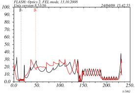
Figure 3: Optics Option II.

In the design of the optics option II we used $k_{0}$ as a weight functions, i.e. we placed the main attention to the relative errors in the quadrupole $k$-values. This was motivated not only by possible uncertainties in the acceleration field distribution along the accelerating modules, but also by uncertainties in knowledge of the transfer coefficients between quadrupole fields and power supply currents.

This optics, which is in operation since spring 2006 and is shown in Fig. 3, reduces the sensitivity to quadrupole errors by a factor of two as compared with the previous optics using criteria (26), but does not show the special behavior of the beta functions in the bunch compressor BC3 and moderately changes the beta functions through the collimator section.

6 CURRENT FLASH OPTICS

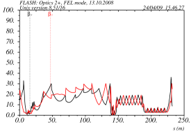
Figure 4: Current FLASH Optics (Optics Option II+).

With the operational experience gained and with almost all quadrupoles being remeasured, now we are much more confident in the setting of transverse focusing. Therefore optics option II was further developed and evolved into a focusing setup which we call optics option II+, and which is shown in Fig. 4. This optics, which is in operations since the beginning of 2008, improves the chromatic beam transfer properties of the optics option II in the DBC2 and SEED sections. In the same time it violates, to a greater or lesser extent, all constraints which were considered as important before the beginning of operations.

7 ACKNOWLEDGEMENT

We thank the colleagues from the FLASH team for their interest in our optics studies and for their help during practical optics setup and measurements. We are specially grateful to H. Mais for the interesting discussion and the careful reading of the manuscript.

References

- [1] V. Ayvazian et al., Eur. Phys. J. D 37 (2006) 297.
- [2] W. Ackermann et al., Nature Photonics 1 (2007) 336.
- [3] V. Balandin, P. Castro, N. Golubeva, Proc. LINAC 2004, Lbeck, Germany, p.360.