Willingness Optimization for Social Group Activity
Abstract
Studies show that a person is willing to join a social group activity if the activity is interesting, and if some close friends also join the activity as companions. The literature has demonstrated that the interests of a person and the social tightness among friends can be effectively derived and mined from social networking websites. However, even with the above two kinds of information widely available, social group activities still need to be coordinated manually, and the process is tedious and time-consuming for users, especially for a large social group activity, due to complications of social connectivity and the diversity of possible interests among friends. To address the above important need, this paper proposes to automatically select and recommend potential attendees of a social group activity, which could be very useful for social networking websites as a value-added service. We first formulate a new problem, named Willingness mAximization for Social grOup (WASO). This paper points out that the solution obtained by a greedy algorithm is likely to be trapped in a local optimal solution. Thus, we design a new randomized algorithm to effectively and efficiently solve the problem. Given the available computational budgets, the proposed algorithm is able to optimally allocate the resources and find a solution with an approximation ratio. We implement the proposed algorithm in Facebook, and the user study demonstrates that social groups obtained by the proposed algorithm significantly outperform the solutions manually configured by users.
1 Introduction
Studies show that two important criteria are usually involved in the decision of a person joining a group activity [8, 14] at her available time. First, the person is interested in the intrinsic properties of the activity, which may be in line with her favorite hobby or exercise. Second, other people who are important to the person, such as her close friends, will join the activity as companions111There are other criteria that are also important, e.g., activity time, and activity location. However, to consider the above factors, a promising way is to preprocess and filter out the people who are not available, live too far, etc.. For example, if a person who appreciates abstract art has complimentary tickets for a modern art exhibition at MoMA, she would probably want to invite her friends and friends of friends with this shared interest. Nowadays, many people are accustomed to sharing information with their friends on social networking websites, like Facebook, Meetup, and LikeALittle, and a recent line of studies [5, 17] has introduced effective algorithms to quantify the interests of a person according to the interest attributes in her personal profile and the contextual information in her interaction with friends. Moreover, social connectivity models have been widely studied [3] for evaluating the tightness between two friends in the above websites. Nonetheless, even with the above knowledge available, to date there has been neither published work nor a real system explores how to leverage the above two crucial factors for automatic planning and recommending of a group activity, which is potentially very useful for social networking websites as a value-added service222The privacy of a person in automatic activity planning can follow the current privacy setting policy in social networking websites when the person subscribes the service. The details of privacy setting are beyond the scope of this paper.. At present, many social networking websites only act as a platform for information sharing and exchange in activity planning. The attendees of a group activity still need to be selected manually, and such manual coordination is usually tedious and time-consuming, especially for a large social activity, given the complicated link structure in social networks and the diverse interests of friends.
To solve this problem, this paper makes an initial attempt to incorporate the interests of people and their social tightness as two key factors to find a group of attendees for automatic planning and recommendation. It is desirable to choose more attendees who like and enjoy the activity and to invite more friends with the shared interest in the activity as companions. In fact, Psychology [8, 14] and recent study in social networks [22, 23] have modeled the willingness to attend an activity or a social event as the sum of the interest of each attendee on the activity and the social tightness between friends that are possible to join it. It is envisaged that the selected attendees are more inclined to join the activity if the willingness of the group increases.
With this objective in mind, we formulate a new fundamental optimization problem, named Willingness mAximization for Social grOup (WASO). The problem is given a social graph , where each node represents a candidate person and is associated with an interest score of the person for the activity, and each edge has a social tightness score to indicate the mutual familiarity between the two persons. Let denote the number of expected attendees. Given the user-specified , the goal of automatic activity planning is to maximize the willingness of the selected group , while the induced graph on is a connected subgraph for each attendee to become acquainted with another attendee according to a social path333For some group activities, it is not necessary to ensure that the solution group is a connected subgraph. Later in Section 2, we will show that WASO without a connectivity constraint can be easily solved by the proposed algorithm with simple modification.. For the activities without an a priori fixed size, it is reasonable for a user to specify a proper range for the group size, and our algorithm can find the solution for each within the range and return the solutions for the user to decide the most suitable group size and the corresponding attendees.444The parameter settings in WASO to fit varied scenarios in everyday life will be introduced in more details in Section 2.2.
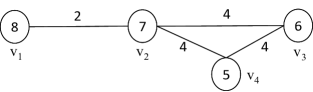
Naturally, to incrementally construct the group, a greedy algorithm sequentially chooses an attendee that leads to the largest increment in the willingness at each iteration. For example, Figure 1 presents an illustrative example with . Node is first selected since its interest score is the maximum one among all nodes. Afterward, node is then extracted. Finally, , instead of , is chosen because it generates the largest increment on willingness, i.e., , and leads to a group with a willingness of . Note the greedy algorithm, though simple, tends to be trapped in a local optimal solution, since it facilitates the selection of nodes only suitable at the corresponding iterations. In this simple example, the above algorithm is not able to find the optimal solution because it makes a greedy selection at each iteration and only chooses as the start node, who enjoys the activity the most at the first iteration, but the optimal solution is {, , } with the total willingness being .
Another approach is to examine the willingness of every possible combination of attendees. However, this enumeration approach needs to evaluate candidate groups, where is the number of nodes in . In current social networking websites, the number of candidate groups is still huge even when we focus on only the candidates located in the same area, e.g., about ten thousand users in British Virgin Islands555http://www.socialbakers.com/facebook-statistics/.. When , the number of candidate groups is in the order of . Thus, this approach is computationally intractable for a massive social network.
Indeed, we show that the problem is challenging and prove that it is NP-hard. As shown in Figure 1, the greedy approach improperly chooses as the start node and explores only a single sequence of nodes in the solution space. To increase the search space, randomized algorithms have been proposed as a simple but effective strategy to solve the problems with large instances [18]. To avoid being trapped in a local optimal solution, a simple randomized algorithm for WASO is to randomly choose multiple start nodes. Each start node is considered as partial solution, and a node neighboring the partial solution is randomly chosen and added to the partial solution at each iteration afterward, until nodes are included as a final solution. This randomized algorithm is more efficient than the greedy approach, because the computation of willingness is not involved during the selection of a node. For the problem with a large , numerous candidate nodes neighboring the partial solution are necessary to be examined in the greedy approach to sum up the willingness, in order to find the one that generates the largest willingness. In contrast, the randomized algorithm simply chooses one neighboring node at random.
With randomization, the aforementioned algorithm is able to effectively avoid being trapped in a local optimal solution. It suffers, however, two disadvantages. Firstly, a start node that has the potential to generate final solutions with high willingness is not invested with more computational budgets for randomization in the following iterations. Each start node in the randomized algorithm is expanded to only one final solution. Thus, a start nodes, which has the potential to grow and become the solution with high willingness, may fail to generate a final solution with high willingness because only one solution is randomly constructed and expanded from the start node. The second disadvantage is that the expansion of the partial solution does not differentiate the selection of the neighboring nodes. Each neighboring node is treated equally and chosen uniformly at random for each iteration. In contrast, a simple way to remedy this issue is to assign the probability to each neighboring node according to its interest score and social tightness of incident edges. However, this assignment is similar to the greedy algorithm in that it limits the scope to the local information corresponding to each node and is not expected to generate a solution with high willingness.
Keeping in mind the above observations in an effort to guide an efficient search of the solution space, we propose two randomized algorithms, called CBAS (Computational Budget Allocation for Start nodes) and CBAS-ND (Computation Budget Allocation for Start nodes with Neighbor Differentiation), to address the above two crucial factors in selecting start nodes and expanding the partial solutions, respectively. This paper exploits the notion of Optimal Computing Budget Allocation (OCBA) [4] in randomization, in order to optimally invest more computational budgets in the start nodes with the potential to generate the solutions with high willingness. CBAS first selects start nodes666The setting of and other parameters is important and will be studied in the end of Section 5. and then randomly adds neighboring nodes to expand the partial solution stage-by-stage, until nodes are included as a final solution. Each start node in CBAS is expanded to multiple final solutions. To properly invest the computational budgets, CBAS at each stage identifies the start nodes worth more computational budgets according to sampled results of the previous stages. Equipped with the allocation strategy of computational resources, CBAS is enhanced to CBAS-ND to adaptively assign the probability to each neighboring node during the expansion of the partial solution according to the cross entropy method. We prove that the allocation of computational budgets for start nodes and the assignment of the probability to each node are both optimal in CBAS and CBAS-ND, respectively. We further show that CBAS can achieve an approximation ratio, while CBAS-ND needs much smaller computational budgets than CBAS to acquire the same solution quality.
The contributions of this paper can be summarized as follows.
-
•
We formulate a new optimization problem, namely WASO, to consider the topic interest of users and social tightness among friends for automatic planning of activities. We prove that WASO is NP-hard. To the best of the authors’ knowledge, there is no real system or existing work in the literature that addresses the issue of automatic activity planning based on both topic interest and social relationship.
-
•
We design Algorithm CBAS and CBAS-ND to find the solution to WASO with an approximation ratio. Experimental results demonstrate that the solution returned by CBAS-ND is very close to the optimal solution obtained by IBM CPLEX, which is widely regarded as the fastest general parallel optimizer, and CBAS-ND is faster than CPLEX.
-
•
We implement CBAS-ND in Facebook and conduct a user study with 137 people. Currently, people are used to organizing an activity manually without being aware of the quality of the organized group, because there is no automatic group recommendation service available for comparison. Compared with the manual solutions, we observe that the solutions obtained by CBAS-ND are 50.6% better. In addition, 98.5% of users conclude that the group recommended by CBAS-ND is better or acceptable. Therefore, this research result has the potential to be adopted in social networking websites as a value-added service.
2 Preliminary
2.1 Problem Definition
Given a social network , where each node and each edge are associated with an interest score and a social tightness score assigned according to the literature [5] and [3] respectively, this paper studies a new optimization problem WASO for finding a set of vertices with size to maximize the willingness , i.e.,
| (1) |
where is a connected subgraph in to encourage each attendee to be
acquainted with another attendee according to a social path in . Notice that the social tightness between and is not necessarily symmetric, i.e., can be different with . Therefore, the willingness in Eq. (1) considers both and . It is worth noting that the illustrating example in the paper is symmetric for simplicity. As
demonstrated in the previous works in Psychology and social networks [22, 23] that jointly consider the social and interest
domains, the willingness of a group is represented as the sum of the topic
interest of nodes and social tightness between them777Different
weights and (1-) can be assigned to the interest scores
and social tightness such that +
.
can be set directly by a user or according to the existing model [23].
The impacts of different will be studied later in Section 5..
Notice that the network with as 0 or as 0 is a special case of WASO. Previous works [8, 14] demonstrated that both social tightness and topic interest are intrinsic criteria involved in the decision of a person to join a group activity, which is in line with the results of our user study presented in Section 5. WASO is challenging due to the tradeoff in interest and social tightness, while the constraint that assures that the is connected also complicates this problem because it is no longer able to arbitrarily choose any nodes from . Indeed, the following theorem shows that WASO is NP-hard.
Theorem 1
WASO is NP-hard.
Proof 2.2.
We prove that WASO is NP-hard with the reduction from Dense -Subgraph (DkS) [9]. Given a graph , DkS finds a subgraph with nodes to maximize the density of the subgraph. In other words, the purpose of DkS is to maximize the number of edges in the subgraph induced by the selected nodes. For each instance of DkS, we construct an instance for WASO by letting , where of each node is set as , and of each edge is assigned as . We first prove the sufficient condition. For each instance of DkS with solution node set , we let . If the number of edges in the subgraph of DkS is , the willingness of WASO is also because . We then prove the necessary condition. For each instance of WASO with , we select the same nodes for , and the number of edges must be the same as . The theorem follows.
2.2 Scenarios
In the following, we present the parameter settings of WASO to fit the need of different scenarios.
Couple and Foe: For any two people required to be selected together, such as a couple, the two corresponding nodes and in are merged into one node with the interest score and social tightness score for each neighboring node of or . Similarly, more people can be merged as well, but the group size is required to be adjusted accordingly. On the other hand, if is a foe of , their social tightness score is assigned a large negative value, such that any group consisting of the two nodes leads to a negative willingness and thereby will not be selected. The relationship of foes can be discovered by blacklists and learnt from historical records. Similarly, is allowed to be assigned a negative value.
Invitation: A piano player plans to hold a small concert. In this case, the player might prefer inviting people that are very good friends with him/her, but it is not necessary for them to be pair-wise acquainted. For this scenario, the activity candidates are the neighboring nodes of , which is denoted as , where represents the inviter (piano player), and we set as 1 for every since the social tightness among the friends may not be important in this scenario.
Exhibition and house-warming party: The British Museum plans to hold an exhibition of Van Gogh and would like to send e-mails to potential visitors. In this scenario, the topic interest is expected to play a crucial role, and is suitable to set as 1 for all . On the other hand, for social activities such as a house-warming party, is 0 for all , and only social tightness is considered.
Separate Groups: The government plans to organize a camping trip on Big Bear Lake to promote environmental protection. In this case, the group does not need to be connected, and a simple way is to add a virtual node to with the interest score of as =+, where is any positive real number. In addition, is connected to every other node with the social tightness score =, and the set of new edges incident to is denoted as . It is necessary to choose so that will connect to multiple disconnected subgraphs to support the above group activities. In this case, nodes need to be included in the final solution.
Now WASO-dis denote the counterpart of WASO without the connectivity constraint. Indeed, WASO-dis is simpler than WASO because the constraint is not incorporated. In the following, we prove that WASO can be reduced from WASO-dis. In other words, any algorithm for WASO can also solve WASO-dis. More specifically, given a graph , WASO-dis finds a subgraph with nodes to maximize the total willingness of the subgraph, i.e., , where is a subgraph in and not required to be a connected subgraph. For any instance of WASO-dis, we construct an instance for WASO by adding a new node as follows. Let =, , where the interest score of is =+ with as any positive real number. In addition, is connected to every other node with the social tightness score =, and the set of new edges incident to is denoted as . Therefore, will appear in the optimal solution of any WASO instance due to its high interest score.
Theorem 2.3.
is the -node optimal solution of any WASO-dis instance if and only if is the -node optimal solution of WASO instance , where .
Proof 2.4.
We first prove the sufficient condition. Since the optimal solution of WASO must include , if is not optimal to WASO, there exists a better solution with , which implies that . Because can act as a feasible solution to WASO-dis, contradicts that is optimal to WASO-dis. Therefore, is the optimal solution to WASO.
We then prove the necessary condition. Since the optimal solution of WASO must include , if is not optimal to WASO-dis, there exists a better solution with , implying that , contradicting that is optimal to WASO because is also a feasible solution to WASO. The lemma follows.
2.3 Related Works
Given the growing importance of varied social networking applications, there has been a recent push on the study of user interest scores and social tightness scores from real social networking data. It has been demonstrated that unknown user interest attributes can be effectively inferred from a social network according to the revealed attributes of the friends [17]. On the other hand, Wilson et al. [21] derived a new model to quantify the social tightness between any two friends in Facebook. The number of wall postings is also demonstrated to be an effective indicator for social tightness [11]. Thus, the above studies provide a sound foundation to quantify the user interest and social tightness scores in social networks. Moreover, Yang [22] and Lee [23] sum up the two factors as willingness for marketing and recommendation. Nevertheless, the above factors crucial in social networks have not been leveraged for automatic activity planning explored in this paper.
Expert team formation in social networks has attracted extensive research interests. The problem of constructing an expert team is to find a set of people owning the specified skills, while the communications cost among the chosen friends is minimized to ensure the rapport among the team members for an efficient operation. Two communications costs, diameter and minimum spanning tree, were evaluated. Several extended models have been studied. For example, each skill needs to contain at least people in order to form a strong team [16], while all-pair shortest paths are incorporated to describe the communications costs more precisely [15]. Moreover, a skill leader is selected for each skill with the goal to minimize the social distance from the skill members to each skill leader [15], while the density of a team is also considered [10].
In addition to expert team formation, community detection as well as graph clustering and graph partitioning have been explored to find groups of nodes mostly based on the graph structure [1]. The quality of an obtained community is usually measured according to the structure inside the community, together with the connectivity within the community and between the rest of the nodes in the graph, such as the density of local edges, deviance from a random null model, and conductance [12]. Sozio et al. [20], for example, detected community by minimizing the total degree of a community with specified nodes. However, the objective function of WASO is different from community detection. Each node and each edge in WASO are associated with an interest score and social tightness score in the problem studied in this paper, in order to maximize the willingness of the attendees with a specified group size, which can be very useful for social networking websites as a value-added service.
3 Algorithm Design for WASO
To solve WASO, a greedy approach incrementally constructs the solution by sequentially choosing an attendee that leads to the largest increment in the willingness at each iteration. However, while this approach is simple, it tends to be trapped in a local optimal solution. The search space of the greedy algorithm is limited because only a single sequence of nodes is explored. To address the above issues, this paper first proposes a randomized algorithm CBAS to randomly choose start nodes. Each start node acts as a seed to be expanded to multiple final solutions. At each iteration, a partial solution, which consists of only a start node at the first iteration or a connected set of nodes at any iteration afterward, is expanded by uniformly selecting at random a node neighboring the partial solution, until nodes are included. We leverage the notion of Optimal Computing Budget Allocation (OCBA) [4] to randomly generate more final solutions from each start node that has more potential to generate the final solutions with high willingness. Later we will prove that the number of final solutions generated from each start node is optimally assigned.
After this, we enhance CBAS to CBAS-ND by differentiating the selection of the nodes neighboring each partial solution. During each iteration of CBAS, each neighboring node is treated equally and chosen uniformly at random. A simple way to improve CBAS is to associate each neighboring node with a different probability according to its interest score and social tightness scores of incident edges. Yet, this assignment is similar to the greedy algorithm insofar as it limits the scope to only the local information associated with each node thereby making it difficult to generate a final solution with high willingness. To prevent the generation of only a local optimal solution, CBAS-ND deploys the cross entropy method according to results at the previous stages in order to optimally assign a probability to each neighboring node.
One advantage of the proposed randomized algorithms is that the tradeoff between the solution quality and execution time can be easily controlled by assigning different , which denotes the number of randomly generated final solutions. Under a given , if start nodes are generated, the above algorithms can optimally divide into parts for the start nodes to find final solutions with high willingness. Moreover, we prove that CBAS is able to find a solution with an approximation ratio. Compared with CBAS, we further prove that the solution quality of CBAS-ND is better with the same computation budget888It is worth noting that randomization is performed only in expanding a start node to a final solution, not in the selection of a start node. This is because the approximation ratio is not able to be achieved if a start node is decided randomly.. The detailed settings of and will be analyzed in Section 5. In addition, the notation table with their impacts on the solution are shown in Table 1.
| Notation | Description | Impact |
|---|---|---|
| social tightness score between node and | set to be a negative value if and are foes | |
| interest score of node | set to be a negative value if does not like the topic | |
| weighting between interest score and tightness score of node | set to be zero if only considers social tightness and one if only concerns topic interest | |
| total computation budget | trade-off between solution quality and computation time | |
| number of start nodes | sampling coverage |
In the following, we first present CBAS to optimally allocate the computational budgets to different start nodes (Section 3.1) and then derive the approximation ratio in Section 3.2. Algorithm CBAS-ND will be presented in Section 4.
3.1 Allocation of Computational Budget for
Start Nodes
Given the total computational budgets specified by users, a simple approach first randomly selects start nodes and then expands each start node to final solutions. However, this homogeneous approach does not give priority to the start nodes that have more potential to generate final solutions with high willingness. In contrast, CBAS optimally allocates more resources to the start nodes with high willingness with the following phases.
-
1.
Selection and Evaluation of Start Nodes: This phase first selects start nodes according to the interest scores and social tightness scores. Afterward, each start node is randomly expanded to a few final solutions. We iteratively select and add a neighboring node uniformly at random to a partial solution, until nodes are selected. The willingness of each final solution is evaluated for the next phase to allocate different computational budgets to different start nodes.
-
2.
Allocation of Computational Budgets: This phase derives the computational resources optimally allocated to each start node according to the previous sampled willingness.
To optimally allocate the computational budgets for each start node, we first define the solution quality as follows.
Definition 3.5.
The solution quality, denoted by Q, is defined as the maximum willingness among all maximal sampled results of the m start nodes,
where is a random variable representing the maximal willingness sampled from a final solution expanded from start node .
Since the maximal sampled result of start node is related to the number of sampling times , i.e., the number of final solutions randomly generated from , the mathematical formulation to optimize the computational budget allocation is defined as
Let denote the start node that are able to generate the solution with the highest willingness. Obviously, the optimal solution in the above maximization problem is to allocate all the computational budgets to . However, since is not given a priori, CBAS divides the resource allocation into stages, and each stage adjusts the allocation of computational budgets to different start nodes according to the sampled willingness from the partial solutions in previous stages.
For each node, phase 1 of CBAS first adds the interest score and the social tightness scores of incident edges and then chooses the nodes with the largest sums as the start nodes. On the other hand, allocating more computational budgets to the start node with a larger sum, similar to the greedy algorithm, does not tend to generate a final solution with high willingness. For this reason, phase 2 evaluates the sampled willingness to allocate different computational budgets to each start node.
In stage of phase 2, let denote the computational budgets allocated to start node at the -th stage. The ratio of computational budgets and allocated to any two start nodes and is
where denotes the best sampled willingness of the partial solutions expanded from start node in the previous stages . Notice that here is the start node that enjoys the highest willingness sampled in the previous stages, is the overall computational budgets allocated to in the previous stages, and denotes the worst sampled willingness of the partial solution expanded from start node in the previous stages. Later, we will prove that the above budgets allocation in each stage is optimal. However, if the allocated computational budgets for a start node is at the -th stage, we prune off the start node in the following -th stage.
Example 3.6.
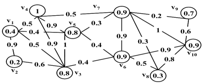
Figure 3 presents an illustrative example for CBAS with , , and . Phase 1 first chooses two start nodes by summing up the topic interest score and the social tightness scores for every node. Therefore, with and with are selected. Next, let , and in this example, and the number of stages is thus Each start node generates samples at the first stage. In the beginning, the node selection probability of start node , i.e., , is set to be ,. The intermediate solution obtained so far is denoted as , and the candidate attendees extracted so far is denoted as . Therefore, the total willingness of is , and . Since the node selection probability is homogeneous in the first stage, we randomly select from to expand . Now the total willingness of is , and . The process of expanding continues until the cardinality of reaches , and we record the first sample result with the total willingness , the worst result of (), and the best result of (). The other sample results from start node are with the total willingness , with the total willingness , with the total willingness , and with the total willingness . The worst and the best results of are updated to and , respectively. After sampling from node , we repeat the above process for start node . The worst result is , and the best result is .
To allocate the computational budgets for the second stage, i.e., , we first find the allocation ratio ==. Therefore, the allocated computational budgets for start nodes and are and , respectively. At the second stage, the best results of and are and , respectively. Finally, we obtain the solution with the total willingness .
3.2 Theoretical Result of CBAS
To correctly allocate the computational budgets to start nodes, we first derive the optimal ratio of computational budgets for any two start nodes. Afterward, we find the probability that node is actually the start node which is able to generate the highest willingness in each stage. Finally, we derive the approximation ratio and analyze the complexity of CBAS.
Definition 3.7.
A random variable, denoted as , is defined to be the sampled value in start node .
The literature of OCBA indicates that the distribution of random variable in most applications is a normal distribution, but the allocation results are very close to the one with the uniform distribution [4, 7]. Therefore, given space constraints, here is first handled as the uniform distribution in [], and the derivation for the normal distribution is presented in Appendix. The probability density function and cumulative distribution function are formulated as
Therefore, for the maximal value ,
Theorem 3.8.
Given the best start node , the probability that exceeds is at most
Proof 3.9.
For
Let equal zero. ( )
It is worth noting that holds in the above equation. Otherwise, the probability that is smaller than will be zero, i.e., . We further change the variables by letting be , and
For ease of reading, we denote as and as . Then the binomial theorem is employed for expanding the polynomial term.
Since , the above equation can be further simplified to
| (2) |
Then, the probability that is better than , i.e.,
With the result above, we allocate the computational budgets by
| (3) |
Since it is impossible to enumerate every final solution expanded from a start node, the ratio of the computational budget allocation is optimal in OCBA [4] if the first equality in Eq. (3) holds. Thus, it is optimal to allocate the computational budgets to and according to the ratio . Notice that if is smaller than , the probability that is smaller than is zero.
Intuitively, the above result indicates that if the best random sample, i.e., , from a start node is small, it is unnecessary to repeat the sampling process too many times since the users nearby the start node are not really interested in the activity or they have an estranged friendship. On the other hand, as the number of sample times increases, it is expected that the identified best start node enjoys the highest willingness.
The following theorem first analyzes the probability that , as decided according to the samples in the previous stages, is actually the start node that generates the highest willingness. Let denote the closeness ratio between the maximum of the start node with the highest willingness and the maximum of other start nodes, i.e., , where generates the maximum willingness among other start nodes. Therefore, in addition to and , is allowed to be any other value from to .
Theorem 3.10.
For WASO with parameter , where is the number of start nodes and is the total computational budgets, the probability that selected according to the previous stages is actually the start node with the highest willingness is at least .
Proof 3.11.
According to the Bonferroni inequality, . In our case, is replaced by to acquire a lower bound for the probability that enjoys the highest willingness. Therefore, by using Theorem 3.8,
Let , where is close to 1. The above equation can be further simplified to .
Given the total budgets , the following theorem derives a lower bound of the solution obtained by CBAS.
Theorem 3.12.
For a WASO optimization problem with -stage computational budget allocation, the maximum willingness from the solution of CBAS is at least , where after stages is , and is the optimal solution.
Proof 3.13.
We first derive the lower bound of as follows. The random variable is denoted as. The cumulative density function is
where for . After exploiting Markov’s Inequality,
We normalize the lower bound and upper bound with and . Let be the top- percentile solution value, i.e. Therefore,
To find the maximum , we let
The maximum is acquired when is . Therefore,
Since is a lower bound of ,
If the computational budget allocation is stages with
, is , which
is
.
Time Complexity of CBAS. The time complexity of CBAS contains two parts. The first phase selects start nodes with time, where is to sum up the interest and social tightness scores, is to build a heap and extract nodes with the largest sum. Afterward, the second phase of CBAS includes stages, and each stage allocates the computation resources with time and generates new partial solutions with nodes for all start nodes. Therefore, the time complexity of the second phase is , and CBAS therefore needs running time.
4 Neighbor Differentiation in
Randomization
4.1 Greedy Neighbor Differentiation
In Section 3.1, CBAS includes two phases. The first phase initiates the start nodes, while the second phase allocates different computational budgets to each start node to generate different numbers of final solutions. During the growth of a partial solution, CBAS chooses a neighboring node uniformly at random at each iteration. In other words, each neighboring node of the partial solution is treated equally. It is expected that this homogeneous strategy needs more computational budgets, because a neighboring node inclined to generate a final solution with high willingness is not associated with a higher probability.
To remedy this issue, a simple algorithm RGreedy (randomized greedy) associates each neighboring node with a different probability according to its interest score and social tightness scores of the edges incident to the partial solution obtained in the previous stage, which is similar to the concept in the greedy algorithm. Given , the ratio of the probabilities that RGreedy selects nodes and at iteration is
where denotes the willingness of the node set . At each iteration, RGreedy randomly selects a vertex in accordance with , until nodes are included.
Intuitively, RGreedy can be regarded as a randomized version of the greedy algorithm with start nodes, while the greedy algorithm is a deterministic algorithm with only one start node. Thus, similar to the greedy algorithm, the assignment of the probability limits the scope to only the local information associated with each node and incident edges. It is envisaged that RGreedy is difficult to generate a final solution with high willingness, which is also demonstrated in Section 5. In contrast, we propose CBAS-ND by exploiting the cross entropy method according to the sampling partial solutions in previous stages, in order to optimally assign a probability to each neighboring node.
4.2 Neighbor Differentiation with Cross Entropy
We enhance CBAS to CBAS-ND to differentiate the selection of a node neighboring each partial solution. Algorithm CBAS is divided into stages. In each stage, it optimally adjusts the computational budgets allocated to each start node according to the sampled maximum and minimum willingness in previous stages. To effectively improve CBAS, CBAS-ND takes advantage of the cross entropy method [19] to achieve importance sampling by adaptively assigning a different probability to each neighboring node from the sampled results in previous stages. In contrast to RGreedy with a greedy-based probability vector assigned to the neighboring nodes, it is expected that CBAS-ND is able to obtain final solutions with better quality. Indeed, later in Section 4.3, we prove that the solution quality of CBAS-ND is better than CBAS with the same computational budget.
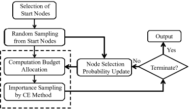
The flowchart of CBAS-ND is shown in Figure 2. We first define the node selection probability vector in CBAS-ND, which specifies the probability to add a node in to the current partial solution expanded from a start node.
Definition 4.14.
Let denote the node selection probability vector
for start node in stage .
= ,…,,…, ,
where is the probability of selecting node for start node in the -th stage.
In the first stage, the node selection probability vector for each start node is initialized homogeneously for every node, i.e. , , . That is, computational budgets are identically assigned to each start node, and the probability associated with every node is also the same. However, different from CBAS and RGreedy, CBAS-ND here examines the top- samples for each start node to generate , so that the node probability will be differentiated according to sampled result in stage .
Definition 4.15.
A Bernoulli sample vector, denoted as , is defined to be the -th sample vector from start node , where is if node is selected in the -th sample and otherwise.
Definition 4.16.
is denoted as the top- sample quantile of the
performances in the -th stage of start node , i.e., =
.
Specifically, after collecting samples generated from for
start node , Node Selection Probability Update in Figure 2 calculates the total willingness
for each sample, and sorts them in the descending order, , while denotes the
willingness of the top- performance sample, i.e. . With those sampled
results, the selection probability of every node in the
second stage is derived according to the following equation,
| (4) |
where the indicator function is defined on the feasible solution space such that is if the willingness of sample exceeds a threshold , and otherwise. Eq. (4) derives the node selection probability vector by fitting the distribution of top- performance samples. Intuitively, if node is included in most top- performance samples in -th stage, will approach 1 and be selected in -th stage.
Later in Section 4.3, we prove that the above probability assignment scheme is optimal from the perspective of cross entropy. Eq. (4) minimizes the Kullback-Leibler cross entropy (KL) distance [19] between node selection probability and the distribution of top- performance samples, such that the performance of random samples in is guaranteed to be closest to the top- performance samples in . Therefore, by picking the top- performance samples to generate the partial solutions in the next stage, the performance of random samples is expected to be improved after multiple stages. Most importantly, by minimizing the KL distance, the convergence rate is maximized.
Moreover, it is worth noting that a smoothing technique is necessary to be included in adjusting the selection probability vector,
to avoid setting or in the selection probability for any node , because will no longer appear or always appear in this case. An example illustrating CBAS-ND is provided as follows. As demonstrated in Section 4.3, the solution quality of CBAS-ND is better than CBAS with the same computation budget.
Example 4.17.
Take Figure 3 as an illustrating example of CBAS-ND. Since CBAS-ND is different from CBAS in the second phase to obtain the node selection probability vector, we continue from the result of the first phase in Section 3, i.e., the allocated computational budgets for start node and are and respectively, and illustrate the second phase of CBAS-ND with Figure 3.
By sorting the willingness samples to , , is equal to Therefore, the samples with the total willingness exceeding include , , and , which are used to update the node selection probability to , . Then, the smoothing technique is adopted with , and the node selection probability becomes
After sampling from node , we repeat the above process for start node . The worst result is , the best result is , and the node selection probability is At the second stage, the best results of and are and , respectively. Finally, we obtain the solution with the total willingness , which is also the optimal solution in this example and outperforms the solution obtained from CBAS.
4.3 Theoretical Result of CBAS-ND
In the following, we prove that the probability assignment with the cross-entropy method [19] in Eq. (4) is optimal. The idea of cross-entropy method originates from importance sampling999Importance sampling [19] is used to estimate the properties of a target distribution by using the observations from a different distribution. By changing the distribution, the ”important” values can be effectively extracted and emphasized by sampling more frequently to reduce the sample variance., i.e., by changing the distribution of sampling on different neighbors such that the neighbors having the potential to boost the willingness are able to be identified and included. Therefore, we first derive the probability of a random sample according to the sampling results in previous stages. After this, we introduce importance sampling and derive the node selection probability vector in the WASO problem to replace the original sampling vector such that the Kullback-Leibler cross entropy (KL) distance between the sampling vector and the optimal importance sampling vector is minimized. Intuitively, a small KL distance ensures that two distributions are very close and implies that the node selection probability vector is optimal because the KL distance between the node selection probability vector in CBAS-ND and optimal node selection probability vector is minimized. Equipped with importance sampling vector, later in this section we prove that the solution quality of CBAS-ND is better than CBAS.
More specifically, let denote the feasible solution space, and is a feasible solution in , i.e., . WASO chooses a group of attendee to find the maximum willingness ,
To derive the probability that the willingness of a random sample exceeds a large value , i.e. , it is necessary for CBAS to generate many samples given that it uniformly selects a neighboring node at random. In contrast, CBAS-ND leverages the notion of importance sampling to change the distribution of sampling on different neighbors. In the following, we first derive the optimal distribution of sampling. First, for the initial partial solution with one start node, let denote the probability density function of generating a sample according a real-valued vector , and is a family of probability density functions on , i.e.,
CBAS can be regarded as a special case of CBAS-ND with the homogeneous assignment on the above vector. A random sample for ,…,,…, is generated with probability , where denotes the probability of selecting node and is the same for all in CBAS. The probability that the willingness of exceeds the threshold is
However, the above equation is impractical and inefficient for a large solution space, because it is necessary to scan the whole solution space and sum up the probability of every sample with . To more efficiently address this issue, a direct way to derive the estimator of is by employing a crude Monte-Carlo simulation and drawing random samples ,…, by to find ,
However, the crude Monte-Carlo simulation poses a serious problem when is a rare event since rare events are difficult to be sampled, and thus a large sample number is necessary to estimate correctly.
Based on the above observations, CBAS-ND attempts to find the distribution based on another importance sampling pdf to reduce the required sample number. For instance, consider a network with nodes, i.e. , and the 2-node group where the maximum willingness is . The expected number of samples with node selection vector in CBAS is larger than the node selection vector of in CBAS-ND. In finer detail, let denote the -th random sample generated by . CBAS-ND first creates random samples ,…, generated by on and then estimates according to the likelihood ratio (LR) estimator ,
| (5) |
Notice that the above equation holds when is infinity, but in most cases only needs to be sufficiently large in practical implementation [6]. Now the question becomes how to derive for importance sampling pdf to reduce the number of samples. The optimal importance sampling pdf to correctly estimate thus becomes
| (6) |
In other words, by substituting with in Eq. (5), holds, implying that only sample is required to estimate the correct , i.e., . However, it is difficult to find the optimal since it depends on , which is unknown a priori and is therefore not practical for WASO.
Based on the above observations, CBAS-ND optimally finds and the importance sampling pdf to minimize the Kullback-Leibler cross entropy (KL) distance between and optimal importance sampling pdf , where the KL distance measures two densities and as
| (7) |
The first term in the above equation is related to and is fixed, and minimizing is equivalent to maximizing the second term, i.e., . It is worth noting that the importance sampling pdf is referenced to a vector . Thus, after substituting in Eq. (6) into the Eq. (7), the reference vector of importance sampling pdf that maximizes the second term of Eq. (7) is the optimal reference vector with the minimum KL distance,
| (8) |
Since is not related to . Eq. (8) is equivalent to
Because it is computationally intensive to generate and compare every feasible , we estimate by drawing samples as
Specifically, CBAS-ND first generates random samples ,…,,…,
where is the -th sample and is a Bernoulli vector
generated by a node selection probability vector , i.e., , where ,…,,…, and denotes
the probability of selecting node . Consequently, the pdf is
To find the optimal reference vector with Eq. (8), we first calculate the first derivative w.r.t. ,
| (9) |
Since can be either 0 or 1, Eq. (9) is simplified to
The optimal reference vector is obtained by setting the first derivative of Eq. (8) to zero.
Finally, the optimal assigned to each node is
Theorem 4.18.
The solution quality of CBAS-ND is better than CBAS under the same computation budget .
Proof 4.19.
Let be the node selection vector in the -th stage, where . We first define the random variables for all , where is the indicator function with 1 if node is in the optimal solution, and otherwise. Then, let denote the probability to generate the optimal solution in the -th stage,
Let be the event that does not sample the optimal solution in the final -th stage. From the previous work [6], the probability for the willingness to converge to the optimal solution can be formulated as
| (10) |
where in Eq. (10) is the smoothing technique parameter. Therefore, since CBAS is identical to CBAS-ND with , the convergence rate that CBAS-ND samples the optimal solution is larger than CBAS. Therefore, to achieve the same solution quality, CBAS-ND requires less computation budget than CBAS. When CBAS runs out of computation budget, i.e., , the computation budget that CBAS-ND achieves the same quality is less than . Let denote the number of stage that CBAS-ND achieves the same quality. Since , we have
Therefore, the solution quality of CBAS-ND is better than CBAS. The theorem follows.
Time Complexity of CBAS-ND. CBAS-ND is different from CBAS in the second phase to find the node selection probability vector, which needs . Therefore, the time complexity of CBAS-ND is . However, in reality we can directly set the probability to for every node not neighboring a partial solution of a start node. Therefore, as shown in Section 5, the experimental result manifests that the execution time of CBAS-ND is not far from CBAS, and both CBAS and CBAS-ND are much faster than RGreedy.
4.4 Discussion
4.4.1 Online computation
In the process of social activity planning, some candidate attendees may not accept the invitations, and an online algorithm to adjust the solution according to user responses can help us handle the dynamic situation. If the online decision of multiple attendees are dependent, the situation is similar to the entangled transactions [13] in databases, in which it is necessary that transactions be processed coordinately in multiple entangled queries. Therefore, we extend CBAS-ND to cope with the dynamic situation as follows. If a user can not attend the activity, it is necessary to invite new attendees. Nevertheless, we have already sent invitations, and some of them have already confirmed to attend. Therefore, CBAS-ND regards those confirmed attendees as the initial solution in the second phase and removes the nodes that can not attend the activity from . Therefore, the node selection probability vector will be updated to identify the new neighbors leading to better solutions according to the confirmed attendees. It is worth noting that the above online computation is fast since the start nodes in the first phase have been decided.
4.4.2 Backtracking
In addition to online computation, we extend CBAS-ND for backtracking to further improve the solution quality as follows. As shown in the previous work [6, 19], the criterion of convergence for Cross-Entropy method is that the node selection probability vector does not change over a number of iterations. Motivated by the above work, given the node selection probability of CBAS-ND at each stage , we derive the difference between and as follows.
When the difference between and is lower than a given threshold , which indicates that the solution quality converges, we backtrack the solution by resetting the node selection probability to and re-sample.
4.4.3 CBAS-ND for Different Scenarios
For the scenarios of couple and foe, invitation, and exhibition, CBAS-ND can be directly applied by modifying the node and edge weights of the graph. For the scenario of separate groups, the start nodes are selected first, and the virtual node is then added to the selection set to relax the connectivity constraint.
5 Experimental Results
In this section, we first present the results of user study and then evaluate the performance of the proposed algorithms with different parameter settings on real datasets.
5.1 Experiment Setup
We implement CBAS-ND in Facebook and invite 137 people from various communities, e.g., schools, government, technology companies, and businesses to join our user study, to compare the solution quality and the time to answer WASO with manual coordination and CBAS-ND for demonstrating the need of an automatic group recommendation service. Each user is asked to plan 10 social activities with the social graphs extracted from their social networks in Facebook. The interest scores follow the power-law distribution according to the recent analysis [5] on real datasets, which has found the power exponent . The social tightness score between two friends is derived according to the widely adopted model based on the number of common friends that represent the proximity interaction [3]. Then, social tightness scores and interest scores are normalized. Nevertheless, after the scores are returned by the above renowned models, each user is still allowed to fine-tune the two scores by themselves. The 10 problems explore various network sizes and different numbers of attendees in two different scenarios. In the first 5 problems, the user needs to participate the group activity and is inclined to choose her close friends, while the following 5 problems allow the user to choose an arbitrary group of people with high willingness. In other words, CBAS-ND in the first 5 problems always chooses the user as a start node. In addition to the user study, three real datasets are tested in the experiment. The first dataset is crawled from Facebook with users in the New Orleans network101010http://socialnetworks.mpi-sws.org/data-wosn2009.html.. The second dataset is crawled from DBLP dataset with nodes and edges. The third dataset, Flickr111111http://socialnetworks.mpi-sws.org/data-imc2007.html., with nodes and edges, is also incorporated to demonstrate the scalability of the proposed algorithms.
In the following, we compare DGreedy, RGreedy, CBAS, CBAS-ND, and IP (Integer Programming) solved by IBM CPLEX in an HP DL580 server with four Intel E7-4870 2.4 GHz CPUs and 128 GB RAM. IBM CPLEX is regarded as the fastest general-purpose parallel optimizer, and we adopt it to solve the Integer Programming formulation for finding the optimal solution to WASO121212Note that because WASO is NP-Hard, it is only possible to find the optimal solutions to WASO with IBM CPLEX in small cases.. The details of Integer Programming formulation is presented in Appendix B.It is worth noting that even though RGreedy performs much better than its counterpart DGreedy and is closer to CBAS and CBAS-ND, it is computation intensive and not scalable to support a large group size. Therefore, we can only plot a few results of RGreedy in some figures. The default is set to be since different -person groups can be partitioned from a network with . With equal , the start nodes averagely cover the whole network. Nevertheless, the experimental analysis manifests that can be set to be smaller than in WASO since the way we select start nodes efficiently prunes the start nodes which do not generate good solutions. The computational budget of CBAS-ND is not wasted much since the start node that do not generate good solutions will be pruned after the first stage. The default cross-entropy parameters and are and respectively, and is as recommended by the cross-entropy method [19]. The results with different settings of parameters will be presented. Since CBAS and CBAS-ND natively support parallelization, we also implemented them with OpenMP for parallelization, to demonstrate the gain in parallelization with more CPU cores.
5.2 User Study
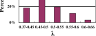
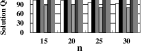
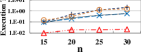
The weights and (1-) in Section 2 for interest scores and social tightness scores are directly specified by the users according to their preferences, and Figure 4(a) shows that the range of the weight mostly spans from 0.37 to 0.66 with the average as 50.3, indicating that both social tightness and interest are crucial factors in activity planning. Figures 4(b)-(e) compare manual coordination and CBAS-ND in the user study. It is worth noting that we generate the ground truth of user study with IP solved by IBM CPLEX to evaluate the solution quality. Figures 4(b) and (c) present the solution quality and running time with different network sizes, where the expected number of attendees is . The user must be included in the group for Manual-i and CBAS-ND-i, and in the other two cases the user can arbitrarily choose a group with high willingness. The result indicates that the solutions obtained by CBAS-ND is very close to the optimal solutions acquired from solving IP with IBM CPLEX. WASO is challenging for manual coordination, even when the network contains only dozens of nodes. It is interesting that is too difficult for manual coordination because some users start to give up thus require smaller time for finding a solution. In addition, WASO is more difficult and more time-consuming in Manual-ni because it considers many more candidate groups.
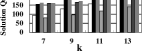
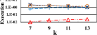
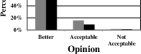
Figures 4(d) and (e) presents the results with different k. The results show that the solution quality obtained by manual coordination with is only 66% of CBAS-ND, since it is challenging for a person to jointly maximize the social tightness and interest. Similarly, we discover that some users start to give up when , and the processing time of manual selection grows when the user is not going to join the group activity. Finally, we return the solutions obtained by CBAS-ND to the users, and Figure 4(f) manifests that 98.5% of users think the solutions are better or acceptable, as compared to the solutions found by themselves. Therefore, it is desirable to deploy CBAS-ND as an automatic group recommendation service, especially to address the need of a large group in a massive social network nowadays.
5.3 Performance Comparison and Sensitivity Analysis
5.3.1 Facebook
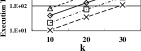
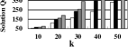
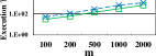
Figure 5(a) first presents the running time with different group sizes, i.e., . RGreedy is computationally intensive since it is necessary to sum up the interest scores and social tightness scores during the selection of a node neighboring each partial solution. Therefore, RGreedy is unable to return a solution within even hours when the group size is larger than . In addition, the difference between CBAS-ND and RGreedy becomes more significant as grows. Figure 5(b) presents the solution quality with different activity sizes, where , , and , respectively. The results indicate that CBAS-ND outperforms DGreedy, RGreedy, and CBAS, especially under a large . The willingness of CBAS-ND is at least twice of the one from DGreedy when . On the other hand, RGreedy outperforms DGreedy since it has a chance to jump out of the local optimal solution.
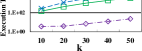
In addition to the activity sizes, we compare the running time of RGreedy, CBAS-ND, and DGreedy with different social network sizes in Figure 5(c) with . DGreedy is always the fastest one since it is a deterministic algorithm and generates only one final solution, but CBAS and CBAS-ND both require less than seconds, whereas RGreedy requires more than seconds. To evaluate the performance of CBAS-ND with multi-threaded processing, Figure 5(d) shows that we can accelerate the processing speed to around times with threads. The acceleration ratio is slightly lower than because OpenMP forbids different threads to write at the same memory position at the same time. Therefore, it is expected that CBAS-ND with parallelization is promising to be deployed as a value-added cloud service.
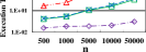
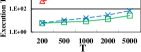
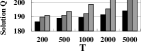
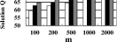
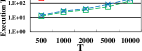
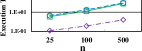
Figures 5(e) and (f) compare the running time and solution quality of three randomized approaches under different total computational budgets, i.e., . As increases, the solution quality of CBAS-ND increases faster than that of the others because it can optimally allocate the computation resources. The running time of CBAS-ND is slightly larger than that of CBAS since CBAS-ND needs to sort and extract the samples with high willingness in previous stages to generate better samples in the following stage. Even though the solution quality of RGreedy is closer to CBAS-ND in some cases, both CBAS and CBAS-ND are faster than RGreedy by an order of .
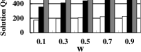
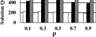
Figure 5(g) presents the solution quality of CBAS-ND with different smoothing technique parameters, i.e., . Notice that the node selection probability vector is homogeneous if we set to zero. The result shows that the best result is generated by for , , and , implying that the convergence rate with is most suitable for WASO in the Facebook dataset. Figure 5(h) compares the top percentile of performance sample value . The result manifests that the solution quality is not inversely proportional to , because for a smaller , the number of samples selected to generate the node selection probability vector decreases, such that the result converges faster to a solution.
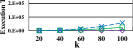
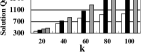
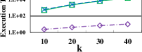
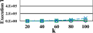
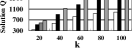
Figures 5(i) and (j) present the running time and solution quality of RGreedy, CBAS, and CBAS-ND with different numbers of start nodes, i.e., . The results show that the solution quality in Figure 5(j) converges when is equal to , which indicates that it is sufficient for to be set as a value smaller than as recommended by OCBA [4]. By assigning in the Facebook dataset, we can reduce the running time to only of the running time in , while the solution quality remains almost the same.
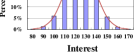
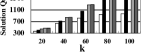
Figure 6(a) shows the interest histogram of random samples on Facebook, which indicates that the distribution follows a Gaussian distribution with the mean as 124.71 and variance as 13.83. The allocation ratio for the variant CBAS-ND-G of CBAS-ND by replacing the uniform distribution with the Gaussian distribution in Theorem 3.8 is derived in Appendix. Figure 6(b) indicates that the solution quality of CBAS-ND and CBAS-ND-G is very close. In contrast to CBAS-ND-G, however, CBAS-ND is more efficient and easier to be implemented because it does not involve the probability integration to find the probability of the best start node.
5.3.2 DBLP
CBAS and CBAS-ND is also evaluated on the DBLP dataset. Figures 7(a) and (b) compare the solution quality and running time. The results show that CBAS-ND outperforms DGreedy by and RGreedy by in solution quality. Both CBAS and CBAS-ND are still faster than RGreedy by an order of . However, RGreedy runs faster on the DBLP dataset than on the Facebook dataset, because the DBLP dataset is a sparser graph with an average node degree of . Therefore, the number of candidate nodes for each start node in the DBLP dataset increases much more slowly than in the Facebook dataset with an average node degree of . Nevertheless, RGreedy is still not able to generate a solution for a large group size due to its unacceptable efficiency.

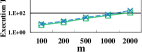
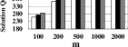
Figures 7(c) and (d) present the solution quality and running time of RGreedy, CBAS, and CBAS-ND with different numbers of start nodes, i.e., . The solution quality of CBAS-ND converges when is , indicating that here it is sufficient to assign as a number much smaller than , because the way we select start node efficiently filter out the start nodes that do not generate good solutions. Compared to in Facebook dataset, CBAS and CBAS-ND need a larger as due to a larger network size in DBLP dataset. Figures 7(e) and (f) compare the solution quality and running time with different . As increases, the solution quality of CBAS-ND also grows faster than the other approaches. Both CBAS and CBAS-ND outperform RGreedy by an order of .
5.3.3 Flickr
Finally, to evaluate the scalability of CBAS and CBAS-ND, Figures 8(a) and (b) compare the solution quality and running time on Flickr dataset. The results show that CBAS-ND outperforms DGreedy by in solution quality when . CBAS and CBAS-ND are both faster than RGreedy in an order of . The trend of running time on Flickr dataset is similar to Facebook dataset, instead of DBLP dataset, because the average node degrees of the Flickr dataset and Facebook dataset are similar. Moreover, RGreedy can support only in the Flickr dataset, smaller than in the DBLP dataset, manifesting that it is not practical to deploy RGreedy in a real massive social network.

5.3.4 Integer Programming and WASO-dis
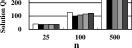
To evaluate the solution quality of CBAS-ND, Figures 9(a) and (b) compare the solution quality and running time of IP (ground truth) with . Since WASO is NP-hard, i.e., the running time for obtaining the ground truth is unacceptably large, we extract 1000 small real datasets from the DBLP dataset with the node sizes as 25, 100, and 500 respectively. The result shows that the solution quality of CBAS-ND is very close to IP, while the running time is smaller by an order of . It is worth noting that CBAS-ND here is single-threaded, but IP is solved by IBM CPLEX (parallel version).
For separate groups, Figure 9(c) first presents the running time with different group sizes, i.e., , where , , and , respectively. For all algorithms, the virtual node is added to the selection set to relax the connectivity constraint. RGreedy computes the incremental willingness of every node in to the selection set , where includes all nodes, and thus are computationally intractable. Therefore, RGreedy is unable to return a solution within hours when the group size is larger than . Figure 9(d) presents the solution quality with different activity sizes. The results indicate that CBAS-ND outperforms DGreedy, RGreedy, and CBAS, especially under a large . In addition, compared to the experimental results in WASO, the difference between CBAS-ND and DGreedy becomes more significant as increases. The reason is that the greedy algorithm selects the node with the largest incremental willingness to the current group and thus is inclined to select a connected group, where the optimal solution may be disconnected.
6 Conclusion and Future Work
To the best of our knowledge, there is no real system or existing work in the literature that addresses the issues of automatic activity planning based on topic interest and social tightness. To fill this research gap and satisfy an important practical need, this paper formulated a new optimization problem called WASO to derive a set of attendees and maximize the willingness. We proved that WASO is NP-hard and devised two simple but effective randomized algorithms, namely CBAS and CBAS-ND, with an approximation ratio. The user study demonstrated that the social groups obtained through the proposed algorithm implemented in Facebook significantly outperforms the manually configured solutions by users. This research result thus holds much promise to be profitably adopted in social networking websites as a value-added service.
The user study resulted in practical directions to enrich WASO for future research. Some users suggested that we integrate the proposed willingness optimization system with automatic available time extraction to filter unavailable users, such as by integrating the proposed system with Google Calendar. Since candidate attendees are associated with multiple attributes in Facebook, e.g., location and gender, these attributes can be specified as input parameters to further filter out unsuitable candidate attendees. Last but not the least, some users pointed out that our work could be extended to allow users to specify some attendees that must be included in a certain group activity.
References
- [1] U. Brandes, D. Delling, M. Gaertler, R. Goerke, M. Hoefer, Z. Nikoloski, and D. Wagner. On modularity clustering. IEEE Transactions on Knowledge and Data Engineering, 20:172–188, 2008.
- [2] W. Bryc. A uniform approximation to the right normal tail integral. In Proc. Appl. Math. Comput., 2002.
- [3] V. Chaoji, S. Ranu, R. Rastogi, and R. Bhatt. Recommendations to boost content spread in social networks. In Proc. WWW, pages 529–538, 2012.
- [4] C. H. Chen, E. Yucesan, L. Dai, and H. C. Chen. Efficient computation of optimal budget allocation for discrete event simulation experiment. IIE Transactions, 42(1):60–70, Jan. 2010.
- [5] A. Clauset, C. R. Shalizi, and M. E. J. Newman. Power-law distributions in empirical data. SIAM Rev., 51(4):661–703, 2009.
- [6] A. Costa, J. Owen, and D. P. Kroese. Convergence properties of the cross-entropy method for discrete optimization. Operations Research Letters, 35(5):573–580, 2007.
- [7] L. Dai, C. H. Chen, and J. R. Birge. Large convergence properties of two-stage stochastic programming. Journal of Optimization Theory and Applications, 106(3):489–510, Sept. 2000.
- [8] M. Deutsch and H. B. Gerard. A study of normative and informational social influences upon individual judgment. Journal of Abnormal and Social Psychology, 51(3):291–301, Nov. 1955.
- [9] U. Feige, D. Peleg, and G. Kortsarz. The dense k-subgraph problem. Algorithmica, 29(3):410–421, 2001.
- [10] A. Gajewar and A. D. Sarma. Multi-skill collaborative teams based on densest subgraphs. In Proc. SDM, 2012.
- [11] E. Gilbert and K. Karahalios. Predicting tie strength with social media. In Proc. CHI, 2009.
- [12] D. F. Gleich and C. Seshadhri. Vertex neighborhoods, low conductance cuts, and good seeds for local community methods. In Proc. KDD, pages 597–605, 2012.
- [13] N. Gupta, L. Kot, S. Roy, G. Bender, J. Gehrke, and C. Koch. Entangled queries: enabling declarative data-driven coordination. In Proc. SIGMOD, 2011.
- [14] M. F. Kaplan and C. E. Miller. Group decision making and normative versus informational influence: Effects of type of issue and assigned decision rule. Journal of Personality and Social Psychology, 53(2):306–313, 1987.
- [15] M. Kargar and A. An. Discovering top-k teams of experts with/without a leader in social networks. In Proc. CIKM, 2011.
- [16] C. Li and M. Shan. Team formation for generalized tasks in expertise social networks. In Proc. of IEEE International Conference on Social Computing, 2010.
- [17] A. Mislove, B. Viswanath, K. P. Gummadi, and P. Druschel. You are who you know: Inferring user profiles in online social networks. In Proc. WSDM, 2010.
- [18] M. Mitzenmacher and E. Upfal. Probability and computing: Randomized algorithms and probabilistic analysis. Cambridge University Press, 2005.
- [19] R. Y. Rubinstein. Combinatorial optimization, cross-entropy, ants and rare events. In S. Uryasev and P. M. Pardalos, editors, Stochastic Optimization: Algorithms and Applications, pages 304–358. Kluwer Academic, 2001.
- [20] M. Sozio and A. Gionis. The community-search problem and how to plan a successful cocktail party. In Proc. KDD, pages 939–948, 2010.
- [21] C. Wilson, B. Boe, A. Sala, K. P. N. Puttaswamy, and B. Y. Zhao. User interactions in social networks and their implications. In Proc. Eurosys, 2009.
- [22] D. N. Yang, W. C. Lee, N. H. Chia, M. Ye, and H. J. Hung. Bundle configuration for spread maximization in viral marketing via social networks. In Proc. CIKM, 2012.
- [23] M. Ye, X. Liu, and W. C. Lee. Exploring social influence for recommendation - a probabilistic generative model approach. In Proc. SIGIR, 2012.
Appendix A Computational Budget Allocation with Gaussian Distribution
In the following, we derive the theoretical results for following the normal distribution with mean and standard deviation of . The probability density function and cumulative distribution function is as follows.
The distribution of maximal value
Therefore, we derive the probability that is smaller than as follows.
As shown above, the probability is necessary to be computed numerically because the function contains function which has no closed-form representation after being integrated. Although we can approximate the function with previous works [2], the function still becomes too complex after raising to the -th or -th power.
Appendix B Integer Programming for WASO
In the following, we describe the Integer Programming (IP) formulation for WASO. Binary variable denotes if node is selected in the solution , and binary variable denotes if two neighboring nodes and are both selected in . The objective function is
where the first term is the total interest score, and the second term is the total social tightness score of the selected nodes. The basic constraints of WASO include
| (11) |
| (12) |
Constraint (11) states that exactly nodes are selected in , while constraint (12) ensures that the social tightness score of any edge can be added to the objective function (i.e., ) only when the two terminal nodes and are both selected (i.e., ); otherwise, are enforced to be .
However, the above basic constraints cannot guarantee that is a connected component of , since nodes are allowed to be chosen arbitrarily. To effective address the issue, we propose the following advanced constraints for WASO to ensure that there is a path from a root node in to every other selected node in , where all nodes in the path must also belong to . More specifically, let binary variable denote if node is the root node, and let binary variable denote if edge in is located in the path from root node to another node in . It is worth noting that since is unknown, variables and in the advanced constraints are correlated to and , respectively.
WASO contains the following advanced constraints.
| (13) |
| (14) |
Constraint (13) states that only one root node will be selected, while constraint (14) guarantees that the selected root node must appear in (i.e, only when ). Equipped with the root node , let denote the set of neighboring node of , let denote the maximal number of edges in the path from to with as the destination of the path, and the following four constraints identify the path from to every node in .
| (15) |
| (16) |
| (17) |
| (18) |
For the selected root node and every other node in (i.e., ), the left hand side (LHS) of constraints 15 and 16 become 1, enforcing that at least one incident edge of and one incident edge of must be included in the path. After obtaining the first and last edge (i.e., and ) in the path from to , constraint 17 is a flow continuity constraint. For each node , if it is an intermediate node in the path, flow continuity constraint states that the flow from to must be identical to the flow to . In other words, constraint 17 chooses a parent node and a child node for in the path
Constraint 18 guarantees that the node sequence in the path contains no cycle; otherwise, for every edge in the cycle, , and the following inequality holds,
and it is thus impossible to find a for every node in the cycle. On the other hand, for any edge with , the constraint becomes redundant since always holds.
The following constraint ensures that every two terminal nodes and of an edge in the path (i.e., ) must participate in (i.e., ).
| (19) |
Therefore, it is not allowed to arbitrarily choose a path in to connect the root node to another node in .