Matlab tools for HDG in three dimensions
Abstract
In this paper we provide some Matlab tools for efficient vectorized coding of the Hybridizable Discontinuous Galerkin for linear variable coefficient reaction-diffusion problems in polyhedral domains. The resulting tools are modular and include enhanced structures to deal with convection-diffusion problems, plus several projections and a superconvergent postprocess of the solution. Loops over the elements are exclusively local and, as such, have been parallelized.
1 Introduction
In this paper we provide some programming tools for full Matlab implementation of the Hybridizable Discontinuous Galerkin (HDG) method on general conforming tetrahedral meshes for fixed but arbitrary polynomial degree. The presentation is detailed on a second order linear reaction-diffusion equation with variable coefficients and mixed boundary conditions, but we also provide the tools to construct the matrices needed for convection-diffusion problems with variable convection, thus creating all necessary blocks to deal with general steady-state problems.
The HDG method originated in a sequence of papers of Bernardo Cockburn and his collaborators, consolidating in the unified framework of [4]. As seen in that paper, the HDG can be considered as a Mixed Finite Element Method (MixedFEM) [2], coded with the use of Lagrange multipliers to weakly enforce the restrictions on interelement faces [1], and then hybridized so that the only global variable is the collection of Lagrange multipliers, that ends up being an optimal approximation of the primal variable on the faces of the triangulation.
Compared with general MixedFEM (programmed in hybridized form), HDG has the advantage of not using degrees of freedom to stabilize the discrete equations, while keeping equal optimal order of convergence in all computed fields. (Stability is obtained through a stabilization parameter.) From this point of view, HDG is a valid option if one is willing to pay the prize of using MixedFEM, for instance, to obtain approximations of more fields of the solution of the problem. In comparison with other FEM, that work directly on the second order formulation, HDG performs well for high orders [9]. For low order methods, HDG can be adopted in situations where either MixedFEM or DG are thought to be advantageous. We will, however, not exploit here the advantages of HDG/DG for having non-conforming meshes or variable degree. Extension of the code to variable-degree methods does not seem to change much, but it requires rethinking the data structures and the vectorization process. Extension to more general meshes would require new tools for the geometric handling that we are not dealing with at this moment. In comparison to other DG methods (mainly those of the Interior Penalty family), HDG requires less degrees of freedom in the solution of the global system, since this has been reduced to the interfaces of the elements. On the positive side as well, HDG does not contain any penalization parameter that needs tuning to obtain convergence. It also has some attractive superconvergence properties that allow for local element-by-element postprocessing à la Stenberg [10].
One goal of the paper is the systematization of the construction of local and global matrices by looping over quadrature nodes and polynomial degrees, avoiding large loops over elements. We partially accomplish this by using Matlab inbuilt functions for Kronecker products, construction of sparse matrices, and vectorization. All loops on elements are purely local and have been parallelized so that they can take advantage of the Matlab Parallel Toolbox. We hope this piece of work will contribute to the popularization of a method that has already a sizeable follow-up, given its good properties. This being Matlab code, we are not expecting the code to run on very large problems, but, as we show in the experiments, we can show reasonably high order of convergence for three dimensional problems, working on a laptop with only two processors. We will also comment on how this code can be easily modified to provide the hybridized implementation of the Brezzi–DOuglas–Marini (BDM) mixed element, which is an alternative to using -conforming bases [6].
Model equations.
Let be a polyhedron with boundary , divided into a Dirichlet and a Neumann part ( and ) such that each part is the union of faces of . The unit outward-poiting normal vector field on is denoted . The model problem we will be discussing in this document is
| (1.1a) | ||||||
| (1.1b) | ||||||
| (1.1c) | ||||||
| (1.1d) | ||||||
The diffusion coefficient is strictly positive, while . (Both of them are functions of the space variables.) The Neumann boundary condition is given in non-standard way, as the normal component of a vector field (of which only the normal component is used), in order to give an easier way to test exact solutions. Modifications for the case of a scalar field are straightforward.
Discrete elements.
The Hybridizable Discontinuous Galerkin method that we will describe here is based on regular tetrahedrizations of the domain. We thus consider a tetrahedral partition of , . The set of all faces in the triangulation is denoted , with the subsets , , corresponding to interior, Dirichlet and Neumann faces. For convenience, we will write
Upon numbering, we can identify elements and faces with respective index sets
This will allow us to write some computational expressions in a format that is very close to their mathematical definition. The local spaces for discretization of and are those of trivariate polynomials of degree up to . The global description of these spaces is
There is a third space, defined on the skeleton of the tetrahedrization:
where is the space of bivariate polynomials of degree not larger than on tangential coordinates. Integral notation will always be given as
Similarly, we will use terms like with , , and . On the boundary of a given element, the normal vector will point outwards. However, when it is clear what the element is, we will simply write .
HDG.
A key ingredient of HDG is a stabilization function. This is a non-negative piecewise constant function on the boundary of each triangle. Thus,
Here is the ordered set of faces of . The function is not single-valued in internal faces. We demand that for each , the function cannot vanish identically, that is, there exists such that . The HDG method works separately each of the equations in (1.1). There are three unknowns: . Locally, we will think of , while will be counted by global face numbering, so we will sometimes refer to values .
| The PDE (1.1a)-(1.1b) is discretized element by element with the equations | ||||||
| (1.2a) | ||||||
| (1.2b) | ||||||
| for all . All the remaining equations are defined (and counted) on edges. We first have flux equilibrium on internal faces: for all , we impose | ||||||
| (1.2c) | ||||||
| This means that the normal numerical flux, , which is an element of for all , is essentially single valued on internal faces, that is on . We finally impose the boundary conditions on Dirichlet faces | ||||||
| (1.2d) | ||||||
| and on Neumann faces , | ||||||
| (1.2e) | ||||||
Equations (1.2) make up for a square system of linear equations. The hybridization of the methods is a static condensation (substructuring) strategy that allows to write the method as a system of equations where only appears as an unknown. For more methods that fit in this framework, see [4]. Theory has been developed in a series of papers, but revisited and deeply reorganized in [5]. Readers acquainted with programming mixed finite element methods will recognized the hybridized form of [1]. (We will come back to this at the very end of the paper.)
2 Geometric structures
Tetrahedra.
All elements will be mapped from the reference tetrahedron with vertices
Note that Given a tetrahedron with vertices (the order is relevant), we consider the affine mapping
| (2.1) |
This map satisfies , All elements of the triangulation will be given with positive orientation, that is,
In this case .
Faces.
A triangle in with vertices (the order is relevant), will be parametrized with
We note that , where is the area of . The local orientation of the vertices of gives an orientation to the normal vector. We will define the normal vector so that its norm is proportional to the area of , that is
Also, if , , then , for .
Boundaries of the tetrahedra.
Given a tetrahedron with vertices we will consider its four faces given in the following order (and with the inherited orientations):
| (2.2) |
(Note that with this orientation of the faces, the normals of the second and fourth faces point outwards, while those of the first and third faces point inwards. This numbering is done for the sake of parametrization.) For integration purposes on , we will use parametrizations of the faces
given by the formulas
| (2.3) |
Consider the affine invertible maps given by the formulas
| (2.4) |
The table on the right shows the indices of the images of the vertices , with boldface font for those that stay fixed. We note that , and change orientation. Take now a tetrahedron , and assume that , i.e., is the face in a global list of faces. We thus have six possible cases of how the parametrizations and match. We will encode this information in a matrix so that
| (2.5) |
We will refer to this matrix as the permutation matrix.
Data structure.
The basic tetrahedrization of (including information on Dirichlet and Neumann boundaries) is given through four fields of a data structure T:
-
•
T.coordinates is an matrix with the coordinates of the vertices of the triangulation.
-
•
T.elements is an matrix, whose -th row of the matrix contains the indices of the vertices of .
-
•
T.dirichlet is an matrix, with the vertex numbers for the Dirichlet faces.
-
•
T.neumann is an matrix, with the vertex numbers for the Neumann faces.
Positive orientation, of listings of vertices for elements and faces, is always assumed, In expanded form, the tetrahedral data structure contains many more useful fields. All these elements can be easily precomputed. It will be useful for what follows to assume that they are easy to access whenever needed.
-
•
T.faces is an matrix with a list of faces: the first three columns contain the global vertex numbers for the faces (its order will give the intrinsic parametrization of the face); Dirichlet and Neumann faces are numbered exacly as in T.dirichlet and T.neumann, the fourth column contains an index:
-
–
0 for interior faces
-
–
1 for Dirichlet faces
-
–
2 for Neumann faces
-
–
-
•
T.dirfaces and T.neufaces are row vectors with the list of Dirichlet and Neumann faces, that is, they point out what rows of T.faces contain a (resp a ) in the last column.
-
•
T.facebyele is an matrix, whose -th row contains the numbers of faces that make up , with the faces given in the order shown in the table in (2.2). Note that this is the matrix we have described as .
-
•
T.perm is an matrix containing numbers from to . Its -th row indicates what permutations are needed for each of the faces to get to the proper numbering of the face, i.e., this is just the matrix .
-
•
T.volume is an column vector with the volumes of the elements.
-
•
T.area is an column vector with the areas of the faces.
-
•
T.normals is an matrix with the non-normalized normal vectors for the faces of the elements; its -th row contains four row vectors of three components each
so that is the normal vector to the face , pointing outwards and such that .
3 Volume integrals
Pseudo-matlab notation.
In order to exploit the vectorization capabilities of Matlab, we will use the following notation to describe some particular operations. First of all, for a function , we will automatically assume that it is vectorized and can thus be simultaneously evaluated in many points stored in equally sizes matrix, so that is a matrix with the same size as , , and . Our default will be that vectors are column vectors. Whenever the sizes of a column vector and a matrix are compatible, we will write and . At the entry level, these are the operations
which can be easily performed using Matlab’s bsxfun utility. Also, the Kronecker product will be used in the following particular situation:
Finally, given a matrix , will be used to denote the row vector corresponding to the -th row of .
Three dimensional quadrature.
To compute or approximate element integrals we will consider a quadrature formula on the reference element :
| (3.1) |
Such formulas can be easily found in the literature [7, 11]. We will find it convenient to store the quadrature points with their barycentric coordinates in a matrix (rows correspond to quadrature points). To integrate on a general element we use the mapping of (2.1) and proceed as follows
| (3.2) |
Piecewise polynomials.
The bases of the local polynomial spaces , containing elements, will be obtained by pushing forward a basis in the reference element. For this we will use the three dimensional Dubiner basis [8], which is given in the enlarged element , where it is -orthogonal. The Dubiner basis is evaluated using a Duffy-type transformation and Jacobi polynomials. What is needed for HDG is the evaluation of the Dubiner basis and of its partial derivatives . We will assume that the basis is ordered in hierarchical form, that is, polynomials of degree are stored after all polynomials of degree for all . We then consider the local bases given by the relations
| (3.3) |
An element of the space will be usually stored as a matrix, where each column contains the coefficients of the local polynomial function in the local basis.
Source terms.
We first extract all nodal information of the grid in three matrices , , . For instance, the element contains the coordinate of the -th node of element . If is the matrix with the barycentric coordinates of the quadrature points in , then
| (3.4) |
are matrices with the coordinates of all quadrature points. Further, let us consider the matrix
| (3.5) |
The computational representation of the formula (see (3.2) and (3.3))
is given by (see (3.4) and (3.5))
where is the column vector containing the volumes of all elements and is a column vector with the weights of the quadrature rule.
Mass matrices.
In order to compute mass matrices with variable density function , we use (3.2)-(3.3) and write
We then evaluate the density at all quadrature points (3.4) to get an matrix, already weighted by the element volumes,
| (3.6a) | |||
| and finally loop over quadrature nodes using the rows of (3.5) | |||
| (3.6b) | |||
The result comes out as a matrix that can be easily reshaped to a array.
Convection matrices.
We start by computing three matrices in the reference element
| (3.7) |
(We assume that the quadrature rule is of sufficiently high order to compute these matrices exactly.) To do this, we require the matrix in (3.5) plus three matrices with derivatives of the basis functions in the reference element
| (3.8) |
Then,
| (3.9) |
Next, we deal with the elements of the associated Piola transform. The elements of the matrices
| (3.10) |
can be computed using the coordinates of the vertices counted by elements (these are the rows of the matrices , , and ) using the formulas:
(Reference to has been dropped to simplify the expression.) A simple change of variables leads to
which, using the matrices (3.9), can be implemented with Kronecker products
| (3.11) |
The result are three matrices.
4 Surface integrals
Integrals on faces.
Two dimensional quadrature rules will be given in the reference element , using points and weights so that
To compute an integral on , we simply parametrize from and proceed accordingly:
For practical purposes, we will keep the barycentric coordinates of the quadrature points in an matrix .
Integrals on boundaries of tetrahedra.
In many cases we will be integrating on a face that is given with geometric information of an adjacent tetrahedron. The quadrature points lead to four groups of quadrature points on the faces of (see (2.3)):
For a given , we can approximate (see (2.4) and (2.5))
| (4.1) |
and thus
| (4.2) |
Note that the use of the permutation index in (4.1) factors out the natural parametrization of on the left, which will be necessary for functions on that are defined by pushing forward functions on , that is, for functions such that we can evaluate .
Bases, faces, and boundaries.
Our starting point is the Dubiner basis [8], which is orthogonal in the enlarged element . We assume it to be given in hierarchical form. The elements of will be described via their coefficients in the basis , where
so that they are stored in form of a matrix (recall that ).
Types of boundary integrals.
There will be three different kinds of integrals on : (a) products of traces of polynomials on , (b) products of piecewise polynomials defined on , (c) products of traces of polynomials of by piecewise polynomials on . Each of these integrals will involve some kind of piecewise constant weight function. Piecewise constant functions on the boundaries of the elements (with different values on internal faces) will be described with matrices. We will be using four examples of this kind of functions:
| (4.3) |
Here is the normal vector on the -th face of , with the normalization (see Section 2). The information of these four piecewise constant functions is readily available in the enhanced geometric data structure.
Type (a) matrices.
Type (b) matrices.
To compute the matrices
we compute the matrices
| (4.7) |
and mix them in the form
| (4.8) |
A simpler option is taking advantage of the fact that the Dubiner basis is orthogonal, so these computations yield diagonal matrices. The result are four matrices. They will be the diagonal blocks of a matrix that will be used in the local solvers.
Type (c) matrices.
Let be a piecewise constant function on the set of boundaries of the elements (in practice, one of the functions described in (4.3)). Let be the piecewise constant functions given by
| (4.9) |
Following (4.1), we can then compute
for , , and . Using (4.5), the matrices
and (4.9), the previous computation reduces to
| (4.10) |
The result is four matrices that are stored as a single array, by stacking the blocks for on top of each other ( on top).
5 Local solvers
Matrices and bilinear forms.
In order to recognize the matrices that we have computed with terms in the bilinear forms of the HDG method, we need some notation. We consider the space
The degrees of freedom for this last space are organized by taking one face at a time in the order they are given by T.facebyele. For (non-symmetric) bilinear forms we will use the convention that the bilinear form is related to the matrix , where is a basis of the space of and is a basis of the space for . This is equivalent to saying that the unknown will always be placed as the left-most argument in the bilinear form and the test function will occupy the right-most location.
Volume terms.
Surface terms.
We next compute all matrices related to integrals on interfaces:
The first of these arrays is , the next four are and the last one is . The first matrix and associated bilinear form (see (4.6)) are
The second one (see (4.10)) corresponds to the bilinear form
or equivalently to , for , , and The matrices associated to the components of the normal vector (see (4.10) again) are related to the bilinear forms
The last matrix (see (4.8)) corresponds to
and is therefore block diagonal. Finally we compute the vectors of tests of with the basis elements of : .
Matrices related to local solvers.
The array and the array with respective slices
| (5.1) |
are the matrix representations of the bilinear forms
given by
We also consider the matrix with columns
| (5.2) |
If is known, we can solve the local problems looking for and , satisfying (1.2a)-(1.2b). Representing with a vector , the matrix representation of this local solution is
| (5.3) |
Note that once the local matrices have been computed, the construction of the three dimentional arrays (5.1) can be easily carried out by stacking the already created three dimensional arrays.
Flux operators.
Consider now the array with slices
| (5.4) |
the array with slices
| (5.5) |
and the matrix with columns
| (5.6) |
The meaning of these matrices can be made clear by looking at boundary fluxes. Given –satisfying equations (1.2a) and (1.2b)–, the HDG method is based on the construction of the flux function
Instead of this quantity, we pay attention to how it creates a linear form
whose matrix representation is
| (5.9) | |||||
| (5.10) |
where is the vector of degrees of freedom of .
Note on implementation.
Construction of the local solvers (5.5) and (5.6), as well as recovery of internal values using (5.3), requires looping over elements. However, this can be easily done in parallel, since at this stage there is no interconnection between elements. Note that we have avoided looping over elements in all previous computations, requiring frequent access to coefficients and geometric features.
6 Boundary conditions and global solver
Dirichlet boundary conditions.
The discrete Dirichlet boundary conditions require finding the decompositions
by solving the system
Using a quadrature rule on the reference element, and parametrizing from it, we have to solve the approximate system
| (6.1) |
Evaluation of the data function at all the quadrature points is done with a similar strategy to the one used for source terms (3.4). We start by organizing nodal information in three (recall that ) matrices , , , each of the containing the corresponding coordinates of the nodes of each of the Dirichlet faces. If is the matrix with the barycentric coordinates of the quadrature points in (Section 4), then the matrices
| (6.2) |
contain the coordinates of the quadrature points on the Dirichlet faces. Using the matrix in (4.7) (see also (4.8)), it is clear that (6.1) can be implemented by solving a system with multiple right-hand sides
| (6.3) |
The result is a matrix.
Neumann boundary conditions.
As opposed to Dirichlet conditions (that are essential in this formulation), Neumann boundary conditions will appear in the right-hand side of the global system. Our goal is to compute the integrals (recall that )
If we consider matrices , , , defined as in (6.2) (but using nodal information for Neumann faces), and if , , are (recall that ) column vectors with the components of the vectors for , then everything is done with the simple computation
| (6.4) |
where . Note that if the Neumann boundary condition is given in a more standard way , then the computation is slightly simpler
where contains the areas of all Neumann faces.
Assembly process.
The local solvers produce a array . We now use the sparse MATLAB builder to assembly the global matrix. The degrees of freedom associated to face are
The degrees of freedom associated to the faces of are thus
We then create two new arrays
The element of has to be assembled at the location . The result is a sparse matrix . This matrix collects the fluxes (5.10) for all the elements, with the result that opposing sign fluxes in internal faces (the normal vector points in different directions) are added. The assembly of the source term, given in the matrix , can be carried out using the accumarray command. The element has to be added to the location . The result is a vector with components. Let us consider the system at its current stage
| (6.5) |
where is the vector containing the elements of in the degrees of freedom corresponding to Neumann faces and zeros everywhere else. This is the matrix representation of the system (1.2) with no Dirichlet boundary conditions, i.e., assuming homogeneous Neumann boundary conditions on , the system having been written in the variable after local inversion of (1.2a)-(1.2b).
Reconstruction.
The solution of the resulting system is . Reconstruction of the other variables is done by solving local problems. In matrix form, we have to solve on each the system
This can be done in parallel.
7 Add-ons
Matrices for convection-diffusion problems.
With very similar techniques, it is easy to compute convection matrices with variable coefficients
| (7.1) |
as well as surface matrices with variable coefficients
These matrices are needed for coding HDG applied to convection-diffusion problems [3], which needs the bilinear forms
Postprocessing.
If we look for such that and for all ,
| (7.3a) | ||||
| (7.3b) | ||||
then it can be shown that this local postprocessed approximation has one additional order of convergence [5]. In order to compute this postprocessing we have to use matrices of the form (7.1) in the right-hand side (using an additional polynomial degree) and we need to compute local stiffness matrices
As in the computation of the convection matrices (3.11), this can be done using geometric vectors and Kronecker products.
Local projections.
For several different purposes, it is also convenient to have some local projections at hand. The first one is the projection on : given we compute such that
Using (3.4) and (3.5), and up to quadrature errors, this projection is easily computed with a single instruction
The projection on
| (7.4) |
is computed using a formula like (6.3)
where we use quadrature points on all faces of the triangulation (see (6.2) for the Dirichlet case).
Error functions.
Once again with very similar ideas it is easy to code the computation of errors
for a given function and approximations and .
HDG projection.
A final projection is directly tied to the HDG method. The input is the collection of a vector field an a scalar function. The output are functions satisfying
| (7.5a) | ||||||||
| (7.5b) | ||||||||
| (7.5c) | ||||||||
It has to be understood that the first two groups of equations are void when . If we construct a mass matrix (with constant unit mass) and drop the last rows (recall that local bases are hierarchical), we obtain a matrix with slices
Using the surface matrices of Section 5, we are led to solve local linear systems with matrices:
The corresponding right-hand sides can be easily constructed using the techniques of previous sections.
BDM.
A hybridized coding of the three dimensional Brezzi-Douglas-Marini element (more properly speaking, this is an element by Brezzi-Douglas-Durán-Fortin, discovered simultaneously by Nédélec) is also easily attainable. For this case, we take , define
and keep as before. The mixed BDM approximation to (1.1) uses equations (1.2) with two simple modifications: , and equation (1.2a) is only tested in . At the implementation level, this means that we only need to redefine the local solvers. Since and the only unknown that is in a smaller space is , we only need to eliminate: the last rows and columns of , the last rows of and , and the last columns of . (This can be done by erasing the corresponding parts of the three dimensional arrays where we have stored the HDG matrices.) All other parts of the HDG code remain untouched.
8 Experiments
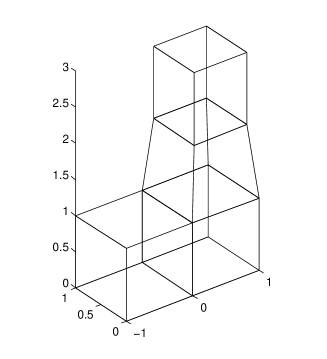
We next give some convergence tests for the method. We take to be the polyhedron sketched in Figure 1. The faces of the polyhedron corresponding to , and conform the Dirichlet boundary . The coarsest triangulation –obtained by a tetrahedral partition of each the four hexahedra shown in Figure 1–, contains elements. Three nested refinements of this partition are used. The main triangulation data are then given in Figure 1. We use variable coefficients:
and take data so that is the exact solution.
| 24 | 192 | 1536 | 12288 | |
| 66 | 456 | 3360 | 25728 |
We test for several values of on the four triangulations. Tables 1–3 show relative errors
| (8.1) |
and relative errors for superconvergent quantities
| (8.2) |
Here: , is the postprocessed solution defined by (7.3), is the projection defined in (7.4) and is the scalar component of the projection defined in (7.5). Theory [5] shows that for smooth solutions, the errors (8.1) behave like while errors (8.2) behave like except when , where they behave like . Estimates of order of convergence for a general quantity are computed using the formula .
| e.c.r. | e.c.r. | e.c.r. | |||
|---|---|---|---|---|---|
| 6.9694e-001 | – | 1.2404e+000 | – | 5.7265e-001 | – |
| 4.2490e-001 | 0.71 | 8.5011e-001 | 0.55 | 3.2710e-001 | 0.81 |
| 2.2749e-001 | 0.90 | 5.0782e-001 | 0.74 | 1.7587e-001 | 0.90 |
| 1.1739e-001 | 0.95 | 2.8336e-001 | 0.85 | 9.1779e-002 | 0.94 |
| e.c.r. | e.c.r. | e.c.r. | |||
|---|---|---|---|---|---|
| 1.3127e+000 | – | 5.4851e-001 | – | 1.2515e+000 | – |
| 6.4689e-001 | 1.02 | 2.9624e-001 | 0.89 | 8.4019e-001 | 0.57 |
| 2.6697e-001 | 1.28 | 1.5688e-001 | 0.92 | 5.0151e-001 | 0.74 |
| 1.1100e-001 | 1.27 | 8.1482e-002 | 0.95 | 2.8027e-001 | 0.84 |
| e.c.r. | e.c.r. | e.c.r. | |||
|---|---|---|---|---|---|
| 1.3607e-001 | – | 4.2677e-001 | – | 1.3580e-001 | – |
| 3.6794e-002 | 1.89 | 1.2953e-001 | 1.72 | 3.1932e-002 | 2.09 |
| 9.6645e-003 | 1.93 | 3.6956e-002 | 1.81 | 7.9337e-003 | 2.01 |
| 2.4878e-003 | 1.96 | 9.9288e-003 | 1.90 | 1.9876e-003 | 2.00 |
| e.c.r. | e.c.r. | e.c.r. | |||
|---|---|---|---|---|---|
| 2.9210e-001 | – | 4.6150e-002 | – | 3.3850e-002 | – |
| 4.5051e-002 | 2.70 | 5.8813e-003 | 2.97 | 4.4054e-003 | 2.94 |
| 6.5777e-003 | 2.78 | 7.6131e-004 | 2.95 | 5.5048e-004 | 3.00 |
| 8.9450e-004 | 2.88 | 9.6512e-005 | 2.98 | 6.8066e-005 | 3.02 |
| e.c.r. | e.c.r. | e.c.r. | |||
|---|---|---|---|---|---|
| 2.7400e-002 | – | 6.5553e-002 | – | 1.9182e-002 | – |
| 4.0693e-003 | 2.75 | 1.1591e-002 | 2.50 | 2.4377e-003 | 2.98 |
| 5.4030e-004 | 2.91 | 1.6402e-003 | 2.82 | 3.0858e-004 | 2.98 |
| 6.8953e-005 | 2.97 | 2.1698e-004 | 2.92 | 3.8901e-005 | 2.99 |
| e.c.r. | e.c.r. | e.c.r. | |||
|---|---|---|---|---|---|
| 2.7092e-002 | – | 4.7030e-003 | – | 4.7177e-003 | – |
| 3.1232e-003 | 3.12 | 3.5134e-004 | 3.74 | 3.5580e-004 | 3.73 |
| 2.1668e-004 | 3.85 | 2.2499e-005 | 3.96 | 2.2835e-005 | 3.96 |
| 1.4237e-005 | 3.93 | 1.3859e-006 | 4.02 | 21.4212e-006 | 4.01 |
We finally test the validity of the HDG method as a -method, by fixing the tetrahedrization (the second one in Figure 1) and increasing from to . We compute the relative errors (8.1) as functions of and check whether the rates
| (8.3) |
as would be expected. Note that the theory for -convergence of HDG is not fully developed. The results are reported in Table 4.
| e.c.r. | e.c.r. | e.c.r. | ||||
|---|---|---|---|---|---|---|
| 0 | 4.2490e-001 | – | 8.5011e-001 | – | 3.2710e-001 | – |
| 1 | 3.6794e-002 | – | 1.2953e-001 | – | 3.1932e-002 | – |
| 2 | 4.0693e-003 | 1.11 | 1.1591e-002 | 0.78 | 2.4377e-003 | 0.90 |
| 3 | 4.4704e-004 | 1.00 | 1.3590e-003 | 1.13 | 1.7465e-004 | 0.98 |
Other easy benchmarks for the method are exact polynomial solutions. These have been tried on the implementation as a way to test exactness of approximation and quadrature in the process.
References
- [1] D. N. Arnold and F. Brezzi. Mixed and nonconforming finite element methods: implementation, postprocessing and error estimates. RAIRO Modél. Math. Anal. Numér., 19(1):7–32, 1985.
- [2] F. Brezzi and M. Fortin. Mixed and hybrid finite element methods, volume 15 of Springer Series in Computational Mathematics. Springer-Verlag, New York, 1991.
- [3] Y. Chen and B. Cockburn. Analysis of variable-degree HDG methods for convection-diffusion equations. Part I: general nonconforming meshes. IMA J. Numer. Anal., 32(4):1267–1293, 2012.
- [4] B. Cockburn, J. Gopalakrishnan, and R. Lazarov. Unified hybridization of discontinuous Galerkin, mixed, and continuous Galerkin methods for second order elliptic problems. SIAM J. Numer. Anal., 47(2):1319–1365, 2009.
- [5] B. Cockburn, J. Gopalakrishnan, and F.-J. Sayas. A projection-based error analysis of HDG methods. Math. Comp., 79(271):1351–1367, 2010.
- [6] V. J. Ervin. Computational bases for and on triangles. Comput. Math. Appl., 64(8):2765–2774, 2012.
- [7] C. A. Felippa. A compendium of FEM integration formulas for symbolic work. Engineering Computations, 21(8):867–890, 2004.
- [8] R. A. Kirby. Singularity-free evaluation of collapsed-coordinate orthogonal polynomials. ACM Trans. Math. Softw., 37(1):Article No. 5, 2010.
- [9] R. M. Kirby, S. J. Sherwin, and B. Cockburn. To CG or to HDG: a comparative study. J. Sci. Comput., 51(1):183–212, 2012.
- [10] R. Stenberg. Postprocessing schemes for some mixed finite elements. RAIRO Modél. Math. Anal. Numér., 25(1):151–167, 1991.
- [11] L. Zhang, T. Cui, and H. Liu. A set of symmetric quadrature rules on triangles and tetrahedra. J. Comput. Math., 27(1):89–96, 2009.