Excitonic effects on coherent phonon dynamics in single wall carbon nanotubes

Abstract

We discuss how excitons can affect the generation of coherent radial breathing modes in the ultrafast spectroscopy of single wall carbon nanotubes. Photoexcited excitons can be localized spatially and give rise to a spatially distributed driving force in real space which involves many phonon wavevectors of the exciton-phonon interaction. The equation of motion for the coherent phonons is modeled phenomenologically by the Klein-Gordon equation, which we solve for the oscillation amplitudes as a function of space and time. By averaging the calculated amplitudes per nanotube length, we obtain time-dependent coherent phonon amplitudes that resemble the homogeneous oscillations that are observed in some pump-probe experiments. We interpret this result to mean that the experiments are only able to see a spatial average of coherent phonon oscillations over the wavelength of light in carbon nanotubes and the microscopic details are averaged out. Our interpretation is justified by calculating the time-dependent absorption spectra resulting from the macroscopic atomic displacements induced by the coherent phonon oscillations. The calculated coherent phonon spectra including excitonic effects show the experimentally observed symmetric peaks at the nanotube transition energies, in contrast to the asymmetric peaks that would be obtained if excitonic effects were not included.

I Introduction

Single wall carbon nanotubes (SWNTs) have been an important material for providing a one-dimensional (1D) model system to study the dynamics and interactions of electrons and phonons. These properties are known to be very sensitive to the SWNT geometrical structure, characterized by the chiral indices $(n,m)$. c471 With rapid advances in ultrafast pump-probe spectroscopy, it has recently been possible to observe lattice vibrations of SWNTs in real time by pump-probe measurements, corresponding to coherent phonon oscillations. gambetta06-cp ; lim06-cpexp ; kato08-cpaligned ; kim09-cpprl ; makino09-cpdoping Femtosecond laser pump pulses applied to a SWNT induce photo-excited electron-hole pairs bound by the Coulomb interaction, called excitons. gambetta06-cp ; kilina07-adv Shortly after the excitons relax to the lowest exciton states ($\approx 10\,{\rm fs}$), the SWNT starts to vibrate coherently by exciton-phonon interactions because the driving forces of the coherent vibration by excitons act at the same time.

The coherent phonon motions can be observed as oscillations of either the differential transmittance or the reflectivity of the probed light as a function of delay time between the pump and probe pulses. By taking a Fourier transformation of the oscillations with respect to time, we obtain the coherent phonon spectra as a function of the phonon frequencies. Several peaks found in the coherent phonon spectra correspond to certain optically active phonon modes. Typical SWNT phonon modes observed from the coherent phonon spectra are similar to those found in the Raman spectra because the exciton-phonon interactions are responsible for both coherent phonon excitations and Raman spectroscopy. However, unlike Raman spectroscopy, ultrafast spectroscopy techniques allow us to directly measure the phonon dynamics, including phase information, in the time domain. gambetta06-cp ; lim06-cpexp ; kim09-cpprl

One of most commonly observed coherent phonon modes in SWNTs is the radial breathing mode (RBM), in which the tube diameter vibrates by initially expanding or contracting depending on the tube types $(\textrm{mod}(n-m,3)=0,1,2)$ and excitation energies. kim09-cpprl Previously we have developed a microscopic theory for the type-dependent generation of coherent RBM phonons in SWNTs within an extended tight binding model and effective mass theory for electron-phonon interactions. sanders09-cp ; nugraha11-cp This model did not take into account the excitonic interaction between the photoexcited electrons and holes. We found that such initial expansion and contraction of the SWNT diameter originates from the wavevector-dependent electron-phonon interactions in SWNTs. Although the coherent phonon generation mechanism neglecting exciton effects considered in previous studies could describe some main features of the coherent phonons in SWNTs, it predicted an asymmetric line shape in contrast to the experimentally observed symmetric line shape. This discrepancy indicates that the presence of excitons in SWNTs should be important microscopically. ando97-exc ; spa04-exc ; wang05-exp ; jiang07-exc

Excitons should have at least four important effects on the generation and detection of coherent phonons in SWNTs: (1) the optical transitions will be shifted to lower energy owing to the Coloumb interaction between the photoexcited electron-hole pair, ando97-exc (2) the strength of the optical transitions will be enhanced since the excitonic wavefunctions have larger optical matrix elements resulting from the localized exciton wavefunctions, jiang07-exphop (3) the phonon interaction matrix elements may also change because the electron-phonon and hole-phonon matrix elements now become exciton-phonon matrix elements, jiang07-exphop and (4) in SWNTs, the excitons can become localized along the tube with a typical exciton size of about $1\,{\rm nm}$. carsten10-exclocal This will change which phonon modes can couple to the photogenerated excitons. Excitons are known to have localized wavefunctions in both real and reciprocal space, jiang07-exc and this should modify the electron-phonon picture of the coherent phonon generation. Due to the localized exciton wavefunctions, the driving force of a coherent phonon is expected to be a Gaussian-like driving force in real space for each localized exciton, whose width is about $1\,{\rm nm}$, instead of a constant force considered in the previous works. sanders09-cp ; nugraha11-cp The localized force can be obtained only if we consider the coupling of excitons and phonons.

The interaction between excitons and coherent phonons will involve many phonon wavevectors for making localized vibrations and many electron (and hole) wavevectors for describing these excitons. By applying strong pump light to the SWNTs, many excitons are generated and the average distances between two nearest excitons are estimated to be about $20\,{\rm nm}$. kamm07-biexciton ; matsuda08-exciton This indicates that the driving force for coherent phonon generation can be approximated by many Gaussians, each of which originates from an exciton and are separated by the distance between two excitons. Using such a driving force model also implies that the coherent phonon amplitudes are inhomogeneous along the nanotube axis. However, since the wavelength of light ($\sim{500\,{\rm nm}}$) is much larger than the spatial modification of the RBM amplitudes, the laser light can only probe the average of the coherent vibrations.

To simulate the exciton effects using coherent phonon spectroscopy, we model the coherent RBM phonon amplitude $Q(z,t)$ as a function of space and time using the Klein-Gordon equation that will be shown to explain the dispersive wave properties. The driving forces are localized almost periodically, and therefore the calculated coherent phonon amplitudes of the RBM are no longer constant along the tube axis. However, by taking an average over the tube length for the calculated coherent phonon amplitudes, we find that the average amplitude fits the oscillations as a function of time observed in the experiments. In order to compare our theory directly with experiments, in which the change of the transmittance $(\Delta T/T)$ or reflectivity $(\Delta R/R)$ is measured, we calculate the time-dependent absorption spectra for macroscopic atomic displacements induced by the coherent phonon oscillations $Q(z,t)$. The symmetric line shape found in the calculated spectra is also consistent with the experimental observations.

This paper is organized as follows. In Section II, we give the phenomenological model for the generation of coherent RBM phonons, which is expressed by the Klein-Gordon equation. The Klein-Gordon equation is able to explain the propagation of the coherent RBM phonons induced by excitons because it gives the RBM phonon dispersion. In Section III, we present the main results and discuss how the inhomogeneous coherent amplitudes obtained from solving the Klein-Gordon equation can lead to the observed homogeneous time-dependent absorption spectra. Finally, we give conclusions in Section IV.

II Coherent phonon model

In the conventional model for the coherent phonon generation mechanism in semiconductor systems, the phonon modes that are typically excited are the ones with phonon wavevector $q=0$. The coherent phonon amplitudes $Q_{\rm c}(t)$ satisfy a driven oscillator equation, stanton94-cpmethod ; merlin97-cp

$$\frac{\partial^{2}Q_{\rm c}(t)}{\partial t^{2}}+\omega_{\rm 0}^{2}Q_{\rm c}(t)=S_{\rm c}(t),$$ (1)

where $\omega_{0}$ is the phonon frequency at $q=0$ and $S_{\rm c}(t)$ is a driving force that depends on the physical properties of a specific material. In the case of a SWNT, without considering the excitonic effects, $S_{\rm c}(t)$ is given by sanders09-cp ; nugraha11-cp

$$S_{\rm c}(t)=-\frac{2\ \omega_{0}}{\hbar}\sum_{\mu k}M_{\rm el-ph}^{\mu}(k)\delta f^{\mu}(k,t),$$ (2)

where $M_{\rm el-ph}^{\mu}(k)$ is the electron-phonon matrix element for the $\mu$-th cutting line (one-dimensional Brillouin zone of a SWNT) as a function of the one-dimensional electron wavevector $k$ and is calculated for each phonon mode at $q=0$. The distribution function $\delta f^{\mu}$ of photo-excited carriers generated by a laser pulse pumping at the $E_{ii}$ transition energy is obtained by solving a Boltzmann equation for the photogeneration process. sanders09-cp

We can see in Eqs. (1) and (2) that $Q_{\rm c}(t)$ and $S_{\rm c}(t)$ have a time dependence only and no spatial dependence when we consider electron-photon (or hole-photon) and electron-phonon (or hole-phonon) interactions, i.e. we ignored the excitonic interaction between the photoexcited electrons and holes. We now extend this model by considering that the exciton effects (exciton-photon and exciton-phonon interactions) give a spatial dependence to the coherent phonon amplitude and to the driving force, which we denote as $Q(z,t)$ and $S(z,t)$, respectively. Here $z$ is the position along the nanotube axis. To describe the coherent phonon amplitude $Q(z,t)$, we propose using the Klein-Gordon equation,

$$\frac{\partial^{2}Q(z,t)}{\partial t^{2}}-c^{2}\frac{\partial^{2}Q(z,t)}{\partial z^{2}}=S(z,t)-\kappa Q(z,t)$$ (3)

where $c$ and $\kappa$ are the propagation speed and dispersion parameter depending on the SWNT structure, respectively. The Klein-Gordon equation is solved subject to the two initial conditions $Q(z,0)=0$ and $\dot{Q}(z,0)=0$. The exciton-induced driving force $S(z,t)$ is given by

$$S(z,t)=-\frac{2}{\hbar}\sum_{\mu,k,q}\omega_{q}M_{\rm ex-ph}^{\mu}(k,q)\delta f^{\mu}(k,t){\rm e}^{{\rm i}qz},$$ (4)

where $M_{\rm ex-ph}^{\mu}(k,q)$ is the exciton-phonon matrix element on the $\mu$-th cutting line as a function of the exciton wavevector $k$ and phonon wavevector $q$. By using the driving force expression of Eq. (4), the amplitude $Q(z,t)$ is dimensionless because the dimension of $S(z,t)$ is the inverse of time square (instead of length per inverse of time square). Here the actual coherent phonon amplitudes with units of length can be obtained by multiplying $Q(z,t)$ with the zero-point phonon amplitude $Q_{0}=\sqrt{\hbar/2M_{\rm c}\omega_{0}}$, where $M_{\rm c}$ is the total mass of the carbon atoms in the nanotube unit cell.

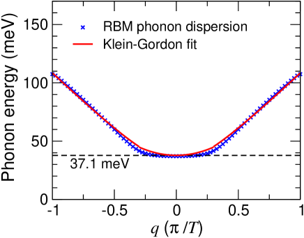
Figure 1: (Color online) RBM phonon dispersion of a (11,0) nanotube. Theoretical data are represented by cross symbols, which are calculated using a force constant model as in Refs. sanders09-cp, and jishi93-phonon, . The solid line shows the fitted RBM dispersion using the Klein-Gordon dispersion relation in Eq. (8). The phonon energy, $\hbar\omega$, is plotted as a function of $q$ in units of $\pi/T$. Here $T=0.431\,{\rm nm}$ is the unit cell length of the $(11,0)$ tube.

The reason why we adopt the Klein-Gordon equation to explain the exciton-induced coherent phonon generation in SWNTs is based on a phenomenological consideration. We generally expect that the coherent RBM phonons are propagating dispersively along the nanotube axis. Integrating $Q(z,t)$ and $S(z,t)$ over $z$ should give $Q_{\rm c}(t)$ and $S_{\rm c}(t)$ in Eq. (1) which describes the homogeneous vibration observed in experiments. Parameters $c$ and $\kappa$ in the Klein-Gordon equation can then be obtained from the RBM phonon dispersion, which gives positive $c$ and $\kappa$ values. To obtain this relationship, we consider the Klein-Gordon equation (3) with $S(z,t)=0$ and take a Fourier transform defined by

$$\tilde{Q}(q,\omega)=\int\limits_{-\infty}^{\infty}\int\limits_{-\infty}^{\infty}Q(z,t){\rm e}^{{\rm i}(qz-\omega t)}{\rm d}{z}{\rm d}{t},$$ (5)

to obtain

$$-\omega^{2}\tilde{Q}+c^{2}q^{2}\tilde{Q}=-\kappa\tilde{Q}.$$ (6)

From Eq. (6) we have a dispersion relation for the Klein-Gordon equation,

$$-\omega^{2}+c^{2}q^{2}=-\kappa.$$ (7)

The physical solution of Eq (7) for $\omega>0$ is

$$\omega(q)=\sqrt{c^{2}q^{2}+\kappa}.$$ (8)

We can then fit the wave dispersion to the RBM phonon dispersion which is already available by force constant or first-principle models. jishi93-phonon ; maul02-phonon ; dubay03-phonon We are particularly interested in the region of $q\ll\pi/T$ ($T$ is the unit cell length of a SWNT c471 ) because this is the typical size over which an exciton in reciprocal space interacts with a phonon. jiang07-exc ; jiang07-exphop Fitting the RBM phonon dispersion to Eq. (8) thus gives the values of both $c$ and $\kappa$ to be used in the Klein-Gordon equation. As for the phonon dispersion shown in Fig. 1, which here is calculated for a $(11,0)$ tube, we obtain $c=2.545\,{\rm nm}/\,{\rm ps}$ and $\kappa=3147.22\,{\rm ps}^{-2}$. Hereafter, we will consider the $(11,0)$ tube as a representative example for the simulation.

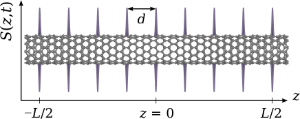
Figure 2: (Color online) Schematic illustration of the driving force $S(z,t)$ created by excitons which align along the nanotube axis. In general, the excitons can be distributed randomly with an average separation between two excitons denoted by $d$. The force $S(z,t)$ is symmetric in the circumferential direction.

To simulate the coherent phonon dynamics, we can further simplify the driving force in Eq. (4), which contains the exciton-phonon matrix element, by assuming that the spatial shape of the driving force follows that of the exciton wavefunction. This is because the exciton-phonon matrix element is the electron-phonon matrix element weighted by the exciton wavefunction coefficients. The spatial shape of the exciton wavefunction can be fitted to a Gaussian with a certain full width at half maximum, $\sigma_{z}$, that also determines the exciton size. The exciton wavefunction with the corresponding exciton energy dispersion can be obtained by solving the Bethe-Salpeter equation. jiang07-exc ; jiang07-exphop

Furthermore, we consider that the Gaussian force appears approximately every $15-30\,{\rm nm}$ along the tube axis depending on the photoexcited carrier density. For example, by solving for the photo-excited distribution $\delta f$ using the method described in Ref. sanders09-cp, , we estimate an exciton density for a $(11,0)$ tube at an excitonic transition energy $E_{22}=1.78\,{\rm eV}$ which is about $5.6\times 10^{-2}\,{\rm nm}^{-1}$. This exciton density corresponds to the average spatial separation between two excitons of about $18\,{\rm nm}$. In this case, we neglect the exciton center-of-mass motion that involves the exciton-exciton interaction, such as would be important for exciton diffusion and the Auger effect, kamm07-biexciton ; matsuda08-exciton ; konabe09-auger which could be considered in a future work.

Before the excitons interact with each other, the optically excited exciton does not have the center-of-mass momentum because of the energy-momentum conservation, and thus we need some more additional time (sub-picoseconds) after the excitation to obtain the finite diffusion constant which affects the coherent phonon dynamics. In a micelle-encapculated nanotube sample, excitons typically diffuse by about $2\,{\rm nm}$ (every $1\,{\rm ps}$), xie12-diff while the average separation between two excitons is one order of magnitude larger. Although in a pristine nanotube sample the excitons can diffuse up to the same order as the average separation between two excitons, maru10-diffusion the exciton diffusion mostly contributes to the decay of the exciton life time. hagen05-decay Also, the Auger rate is on the order of $0.1\,{\rm ps}^{-1}$, which corresponds to the ionization or recombination times of excitons of about $10\,{\rm ps}$, onoda11 whereas the time needed for generating coherent phonons in our case is as early as hundred femtoseconds (the phonon period) and the time scale for considering the coherent phonon dynamics is less than $5\,{\rm ps}$. The Auger effect is then important in later time when any two excitons can collide and disappear. If the two excitons survive, the coherent phonon amplitude may be given by a linear combination of amplitudes induced by each exciton. However, we did not consider such situations for simplicity. Therefore, in the present study, the total driving force for the coherent phonon dynamics can be defined as a summation of contributions from each Gaussian generated from an exciton.

Each Gaussian function centered at the exciton position $z_{i}$, which is distributed along the tube axis, is expressed as

$$S_{i}(z,t)=A_{g}e^{-(z-z_{i})^{2}/2\sigma_{z}^{2}}\theta(t),$$ (9)

where $\theta(t)$ is the Heaviside step function, $A_{g}$ is the force magnitude obtained from the product of the exciton-phonon interaction and the related factors in Eq. (4), and $\sigma_{z}$ is the width of the exciton-phonon matrix element for a given $(n,m)$ SWNT. A typical value of $\sigma_{z}$ is related to the exciton size in real space ($\sim 1\,{\rm nm}$). The exciton wavefunctions, exciton energies, exciton-photon and exciton-phonon matrix elements are all calculated by solving the Bethe-Salpeter equation within the extended tight-binding method as developed by Jiang et al. jiang07-exc ; jiang07-exphop The force magnitude thus obtained is on the order of $10^{3}\,{\rm ps}^{-2}$. For the lowest $E_{22}$ exciton state of the $(11,0)$ tube, we obtain $\sigma_{z}=0.9\,{\rm nm}$ and $A_{g}=4.82\times 10^{3}\,{\rm ps}^{-2}$. The total driving force used in solving Eq. (3) is a summation of Gaussian forces in terms of Eq. (9),

$$S(z,t)=\sum_{i=1}^{N}S_{i}(z,t),$$ (10)

where $N$ is the number of excitons (and thus the number of Gaussian forces) in a SWNT. In Fig. 2, we show a schematic diagram of a typical model for our simulation. The driving force $S(z,t)$ has an axial symmetry and is aligned along the nanotube axis with a separation distance of $d$. To avoid any motions of the center of mass, the general force $S({\bm{r}},t)$ should also satisfy a sum rule,

$$\int\limits_{-\infty}^{\infty}S(\bm{r},t){\rm d}{\bm{r}}=0,$$ (11)

which is automatically satisfied for $S(z,t)$ in Eq. (10) because of the axial symmetry of the model, as can also be understood from Fig 2. In the present calculation, we fix $d=18\,{\rm nm}$, and there are $N=9$ narrow Gaussian forces arranged periodically (thus $L=144\,{\rm nm}$). The RBM phonon energy near $q=0$ is $37.1~{}\,{\rm meV}$, corresponding to a frequency $\omega=297\,{\rm cm}^{-1}$ and a vibration period $\tau=0.112~{}\,{\rm ps}$.

It should be noted that the specific details of the spatial arrangement of the localized excitons are also mainly determined by the exciton-exciton interaction. kamm07-biexciton ; matsuda08-exciton ; konabe09-auger However, we can simply take into account the main point resulting from these exciton-exciton interactions that the excitons will be stabilized and will arrange themselves in a certain spatial configuration. In general, excitons do not need to be arranged periodically and can be distributed randomly along the tube axis. Here we use a specific exciton configuration as a representative example that corresponds to a slightly random configuration of excitons. Interestingly, it will be justified in the next section that even if the excitons are distributed very randomly along the tube axis, the coherent phonon amplitudes at each exciton site are not affected as far as two (or more) excitons are not located at the same position.

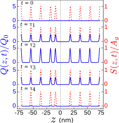
Figure 3: (Color online) Time evolution of coherent phonon amplitudes in a $(11,0)$ nanotube for a slightly random distribution of excitons with an average separation $d=18\,{\rm nm}$ and with the center force shifted by $9\,{\rm nm}$. Solid lines show snapshots of $Q(z,t)$ as a function of $z$ (position along the tube axis) for several different $t$ values with a time sequence $\tau_{j}=j\tau/4$, where $\tau=0.112\,{\rm ps}$ is the fundamental period. $Q(z,t)$ is plotted in terms of $Q_{0}=2.59\times 10^{-3}\,{\rm nm}$. Dotted lines show the force $S(z,t)$ for comparison.

III Results and Discussion

In Fig. 3, we plot the coherent RBM phonon amplitudes $Q(z,t)$ for a $(11,0)$ nanotube pumped at its $E_{22}$ transition energy, in which a snapshot is taken for $t=0$ to $\tau_{4}$, where $\tau_{j}=j\tau/4$. We consider a slightly random configuration of excitons with an average distance between two excitons $d=18\,{\rm nm}$ and then we shift one of the excitons at the center of the tube axis by $9\,{\rm nm}$. The calculation is done numerically by solving for $Q(z,t)$ from Eq. (3) with periodic boundary conditions at $\pm L/2$. We can observe some periodic peaks corresponding to each localized force and these peaks also do not move as a function of time. One might then ask whether or not such exciton effects correctly describe the coherent phonon oscillations in SWNTs. This can be answered by considering the average of the inhomogeneous $Q(z,t)$ per nanotube length.

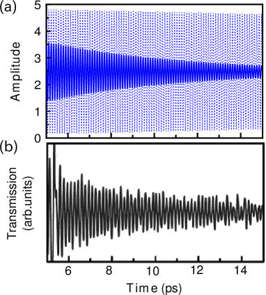
Figure 4: (Color online) (a) Average of coherent phonon amplitudes per length, $A(t)$, plotted as a function of time for a $(11,0)$ nanotube ($\tau=0.112\,{\rm ps}$) and shown in units of $Q_{0}=2.59\times 10^{-3}\,{\rm nm}$. The dotted line represents the average amplitude for the force distribution shown in Fig. 3. The solid line represents the average amplitude if a decay constant $0.2\ {\rm ps^{-1}}$ is taken into account. (b) An example of the transmission oscillation data available for a $(13,3)$ tube measured in a pump-probe experiment with $\tau=0.162\,{\rm ps}$ (reproduced from Ref. kim09-cpprl, ). The average coherent phonon amplitude shown in (a) resembles the oscillating feature of the experimental transmission shown in (b).

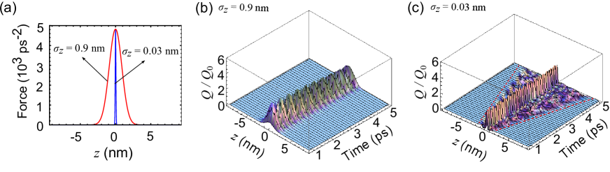
Figure 5: (Color online) (a) Driving forces with two different parameters $\sigma_{z}(=0.9\,{\rm nm})>\sigma_{zc}$ and $\sigma_{z}(=0.03\,{\rm nm})<\sigma_{zc}$, which give (b) only localized and (c) both localized and propagating wave components, respectively. For the $(11,0)$ tube in this simulation, we have $\sigma_{zc}=0.045\,{\rm nm}$. The propagating wave components in (c) travel with a speed of $1.68\,{\rm nm}/\,{\rm ps}$.

To clarify that our model can describe homogeneous coherent RBM phonon oscillations that are observed in experiments, lim06-cpexp ; kim09-cpprl we define an average of $Q(z,t)$ as follows

$$A(t)=\frac{1}{L}\int_{L}Q(z,t){\rm d}z.$$ (12)

In Fig. 4(a), we plot $A(t)$ for the $(11,0)$ tube considered above. We also include a decay constant $0.2\ {\rm ps^{-1}}$ to resemble the experimental results. kim09-cpprl Interestingly, now the coherent phonon amplitudes, which have been averaged before, could fit the experimental shape of the homogeneous transmission oscillation in Figs. 4(b). We then interpret that such an experiment cannot observe the nanoscopic vibration of the exciton effects on the coherent phonon amplitudes, but it can only observe the averaged amplitudes. Moreover, the definition (12) is important mathematically to describe the homogeneous coherent phonon amplitudes in experiments if we are able to recover Eq. (1) from the Klein-Gordon equation (3). Indeed, by integrating both left and right sides of Eq. (3),

$$\int_{L}Q_{tt}{\rm d}z-\int_{L}c^{2}Q_{zz}{\rm d}z=-\int_{L}\kappa Q{\rm d}z+\int_{L}S{\rm d}z,$$

and using $\int_{L}Q_{tt}{\rm d}z=A_{tt}$, $\int_{L}\kappa Q{\rm d}z=\kappa A$, $\int_{L}Q_{zz}{\rm d}z=0$, we can obtain

$$A_{tt}+\kappa A(t)=S(z),$$ (13)

which is nothing but the driven oscillator model in Eq. (1).

It is important to note that we have assumed a certain configuration of excitons as a function of $z$. However, excitons in nature might not be uniformly spaced and any exciton distributions with random spacing can be possible. Nevertheless, we expect that our result for the average amplitude $A(t)$ in Fig. 4 is approximately constant regardless of the exciton spacing, as far as the average exciton density remains the same. This can be rationalized by considering a trial solution of the Klein-Gordon equation,

$$Q(z,t)={\rm e}^{-\lambda z}{\rm e}^{i(qz-\omega t)},$$ (14)

which comprises a travelling wave and a decay term with parameter $\lambda$ to be determined. By substituting Eq. (14) into Eq. (3) and setting $S(z,t)=0$, we obtain

$$\lambda=iq\pm\sqrt{\frac{\kappa}{c^{2}}-q^{2}},$$ (15)

where we have assumed $\omega=qc$ and the sign $\pm$ is determined for the $\pm z$ region. Depending on whether the value of $\sqrt{\kappa/c^{2}-q^{2}}$ is real or pure imaginary, respectively, we can get a spatially localized or propagating solution of $Q(z,t)$. In the presence of a force, we can solve Eq. (3) using the Green’s function method for a single Gaussian force $S(z,t)=A_{g}{\rm e}^{-z^{2}/2\sigma_{z}^{2}}\theta(t)$. The solution for $Q(z,t)$ in the region $-L/2<z<L/2$ with a boundary condition, $Q(-L/2,t)=Q(L/2,t)$, is given by

$$\displaystyle Q(z,t)= \frac{2\sigma_{z}A_{g}\sqrt{2\pi}}{L}\sum_{n=0}^{\infty}\bigg{[}\frac{{\rm e}^{-q_{n}^{2}\sigma_{z}^{2}/2}}{c^{2}q_{n}^{2}+\kappa}\times\bigg{(}\cos(q_{n}z)$$

$$\times(1-\cos(t\sqrt{c^{2}q_{n}^{2}+\kappa}))\bigg{)}\bigg{]},$$ (16)

where $q_{n}=n\pi/L$. This solution consists of a wavepacket of standing waves weighted by a Gaussian distribution and a denominator which comes from the phonon dispersion relation of Eq. (8). The Gaussian distribution originates from the Fourier transform of the Gaussian force in real space. In this case, the selection of $q$ is determined by the Fourier transform of the driving force $S(z,t)$. For the Gaussian force in our model, the $q$ value can be selected for the region $0<q<1/\sigma_{z}$. If the maximum $q=1/\sigma_{z}$ is smaller than $q_{\rm c}=\sqrt{\kappa}/c$, then $Q(z,t)$ is localized. If $1/\sigma_{z}$ is larger than $q_{\rm c}$, then $Q(z,t)$ is divided into two contributions: $0<q<q_{\rm c}$ and $q_{c}\leq q<1/\sigma_{z}$, in which the former $q$ value gives the localized wave and the latter part gives the propagating wave. We can then define a critical parameter $\sigma_{z{\rm c}}=1/q_{c}$ to explain the localization or propagation of the coherent phonons obtained from the Klein-Gordon equation.

For the (11,0) tube, we have a critical parameter $\sigma_{z{\rm c}}=(2.545/\sqrt{3147.22})\,{\rm nm}=0.045\,{\rm nm}$. Since in our simulation we already used $\sigma_{z}=0.9\,{\rm nm}$ which is much larger than $\sigma_{z{\rm c}}$, it is then expected that the coherent phonon is sufficiently localized. To emphasize this fact, we show two different cases of Klein-Gordon waves in Fig. 5 for $\sigma_{z}=0.9\,{\rm nm}$ and $\sigma_{z}=0.03\,{\rm nm}$. Figure  5(a) shows the two forces with different $\sigma_{z}$ values, while Figs. 5(b) and (c) shows the corresponding coherent phonon amplitudes that are generated. It can be seen that we obtain localized (propagating) waves by using $\sigma_{z}>\sigma_{z{\rm c}}$ ($\sigma_{z}<\sigma_{z{\rm c}}$). Intuitively, we can understand from Fig. 5(c) that a faster appearance of an amplitude propagating along the $z$ direction can be obtained when $\sigma_{z}$ becomes much smaller than $\sigma_{z{\rm c}}$ although some parts of $Q(z,t)$ remain localized (contribution from $0<q<q_{\rm c}$). The propagating wave components in Fig. 5(c) travel with a velocity $\sqrt{\kappa}/q$, where $q$ in this case is related to $\sigma_{z}$ directly by $q=1/\sigma_{z}$, thus giving a speed of $\sqrt{3147.22\,{\rm ps}^{-2}}\times 0.03\,{\rm nm}=1.68\,{\rm nm}/\,{\rm ps}$. In contrast, in the case of $\sigma_{z}$ much larger than $\sigma_{z{\rm c}}$ [e.g. Fig. 5(b)], we cannot see any amplitudes along the $z$ direction except in a limited region where the force exists, i.e. the propagating wave components cannot be observed. Indeed, the actual RBM dispersion is a bit flatter than the approximation from the Klein-Gordon wave dispersion (see Fig. 1). This means that the modes are localized even more. Therefore, in our case of $\sigma_{z}=0.9\,{\rm nm}$, each excitonic force will not interfere with neighboring force sites separated by distance $d$, which indicates that the average amplitude $A(t)$ in Fig. 4 is not affected by a random separation between every excitonic force. In general, we may say that the localized vibration is a characteristic of the optical phonon propagation driven by a localized force because the wavepacket is dominated by $q\approx 0$ phonons, while the contribution of the group velocity comes from $q\geq q_{\rm c}$. This optical phonon feature differs from that of the acoustic phonon feature whose solution is expressed in terms of traveling waves. sanders01

We then calculate the optical absorption spectra as a function of time using the calculated $Q(z,t)$. It is expected that the inhomogeneous coherent phonon oscillations induce a macroscopic atomic displacement which modifies the transfer integral and thus modulates the energy gap. We calculate the absorption coefficient $\alpha(E_{\rm L},t)$, where $E_{\rm L}$ is the laser excitation energy, by evaluating it in the dipole approximation using Fermi’s golden rule. The absorption coefficient at a photon energy $E_{\rm L}$ obtained by including exciton effects is given by elliot57-absexc ; konabe09-auger

$$\alpha(E_{\rm L},t)= \frac{8e^{2}}{E_{\rm L}Rm_{0}c_{0}}\sum_{\mu k}\ \arrowvert M_{\rm ex-op}^{\mu}\arrowvert^{2}$$

$$\times\delta f^{\mu}(k,t)\ \delta\left(E_{ii}(t)-E_{\rm L}\right),$$ (17)

where $M_{\rm ex-op}^{\mu}$ is the exciton-photon matrix element within the dipole approximation, corresponding to the transition between the initial and final state on the $\mu$-th cutting line, $R$ is the tube radius, $m_{0}$ is the electron mass, and $c_{0}$ is the speed of light. The exciton energy $E_{ii}$ is now time-dependent because of the change in transfer integral due to coherent RBM phonon vibrations $A(t)$.

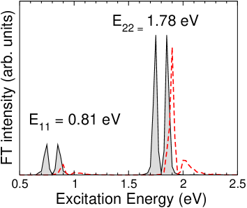
Figure 6: (Color online) Fourier transform intensity of the time-dependent absorption coefficient for the coherent RBM phonon of a (11,0) nanotube as a function of excitation energies $E_{\rm L}$. The solid line represents the coherent phonon spectra which include excitonic effects, showing a symmetric double-peaked line shape at each transition energy $E_{ii}$. The dashed line represents the coherent phonon spectra without excitonic effects, in which asymmetric line shapes were obtained previously. sanders09-cp

Since the bandgap is inversely proportional to the diameter oscillation (or to the coherent RBM amplitudes), the time-dependent absorption $\alpha(E_{\rm L},t)$ has the same oscillating feature as the average amplitude $A(t)$. However, exciton effects acting on the absorption spectrum will modify the shape of the absorption spectra compared to that obtained without inclusion of the exciton effects. We should then calculate the time-dependent absorption for a broad range of excitation energies, for example, within the range of $0.5$ to $2.5\,{\rm eV}$. By performing a Fourier transformation numerically over this energy range, we can obtain the RBM coherent phonon spectra as shown in Fig. 6, which include $E_{11}$ and $E_{22}$ for the $(11,0)$ tube that we consider. The coherent phonon spectra given in Fig. 6 show double-peaked structures as a function of the excitation energies, either with or without including the excitonic effects, as indicated by the solid and dashed lines in Fig. 6, respectively.

The reason for the presence of the double-peak features (either symmetric or asymmetric) in the excitation-dependent coherent phonon intensity can be explained as follows. The generation of coherent RBM phonons modifies the electronic structure of SWNTs and thus it can be detected as temporal oscillations in the transmittance of the probe beam. Since the RBM is an isotropic vibration of the nanotube lattice in the radial direction, i.e. the diameter periodically oscillates at the RBM frequency, this makes the band gap $E_{g}$ also oscillate at the same frequency. As a result, interband transition energies oscillate in time, leading to ultrafast modulations of the absorption coefficients at the RBM frequency, which is also equivalent to the oscillations in the probe transmittance, and thus correspondingly, the excitation energy dependence of the coherent phonon intensity shows a derivative-like behavior. More explicitly, the effect on the absorption $\alpha$ for small changes in the gap can be modeled by kim13-cp

$$\alpha(E_{\rm L}-E_{g})\approx\alpha(E_{\rm L}-E_{g}^{0})-\frac{\partial\alpha(E_{\rm L}-E_{g}^{0})}{\partial E_{\rm L}}\delta E_{g}+\ldots,$$ (18)

which gives

$$\ \Delta\alpha\approx-\frac{\partial\alpha(E_{\rm L}-E_{g}^{0})}{\partial E_{\rm L}}\delta E_{g},$$ (19)

where $E_{g}$ is assumed to be time-dependent, and $\delta E_{g}$ here corresponds to a small change in the bandgap. Since the coherent phonon intensity is obtained by taking the Fourier transform (power spectrum) of the differential transmission, the coherent phonon intensity is thus proportional to the square of the derivative of the absorption coefficient.

The excitonic absorption coefficient basically has a symmetric lineshape with a single peak. spa04-exc Therefore, the derivative of the excitonic absorption coefficient will give a symmetric double-peak feature, in contrast to the asymmetric lineshape expected from the 1D van Hove singularity (joint density of states). Here the use of the Klein-Gordon equation which gives nonhomogeneous macroscopic atomic displacements is then also justified by obtaining the symmetric line shape for the coherent phonon spectra. On the other hand, in the free carrier model without the excitonic effects, we see an asymmetric double-peaked structure at each transition with the stronger peak at lower energy and the weaker peak at higher energy, which originate from the derivative of the asymmetric lineshape of the absorption coefficient. Moreover it has also been noted in some earlier works that the transition energy was shifted upward by several hundred meV. spa04-exc ; kim13-cp

As a final remark, we would like to mention that considering the localized excitons in this work might be just one possibility that gives the symmetric peak of the absorption spectrum because the origin of the symmetric absorption lineshape is basically from the presence of discrete energy levels of excitons in carbon nanotubes. In this sense, if there are other configurations of excitons in carbon nanotubes, which are not localized, such cases might also give rise to the symmetric absorption lineshape. This can be an open issue for future studies. However, we expect that as an initial condition of the system after the excitation by the pump pulse, the excitons should be localized with a certain average separation. chang04-locexc ; hirori06-locexc ; hogele08-locexc

IV Conclusion

We have shown that excitonic effects modify the coherent phonon amplitudes in SWNTs as described by the Klein-Gordon equation. The localized exciton wavefunctions result in an almost periodic and localized driving force in space. Although the exciton effects make the amplitudes inhomogeneous, these amplitudes might be difficult to observe in experiments where the long wavelength of the probe pulse averages over the sample. We then defined a spatial average of the amplitudes that matches the experimental results. Such an interpretation becomes necessary and fundamental since we may say that the pump-probe experiments on coherent phonons could not measure the “real” coherent phonon amplitudes of SWNTs. What is measured in the experiments is actually the average of the amplitudes. Nevertheless, using the present treatment we have been able to simulate the experimental observation of a symmetric double-peaked structure as is observed in the coherent phonon spectra as a function of excitation energy.

References

- (1) R. Saito, M. Fujita, G. Dresselhaus, and M. S. Dresselhaus, Phys. Rev. B 46, 1804–1811 (1992).
- (2) A. Gambetta, C. Manzoni, E. Menna, M. Meneghetti, G. Cerullo, G. Lanzani, S. Tretiak, A. Piryatinski, A. Saxena, R. L. Martin, and A. R. Bishop, Nat. Phys. 2, 515–520 (2006).
- (3) Y. S Lim, K. J. Yee, J. H. Kim, E. H. Haroz, J. Shaver, J. Kono, S. K. Doorn, R. H. Hauge, and R. E. Smalley, Nano Lett. 6, 2696–2700 (2006).
- (4) K. Kato, K. Ishioka, M. Kitajima, J. Tang, R. Saito, and H. Petek, Nano Lett. 8, 3102–3108 (2008).
- (5) J.-H. Kim, K.-J. Han, N.-J. Kim, K.-J. Yee, Y.-S. Lim, G. D. Sanders, C. J. Stanton, L. G. Booshehri, E. H. Hároz, and J. Kono, Phys. Rev. Lett. 102, 037402 (2009).
- (6) K. Makino, A. Hirano, K. Shiraki, Y. Maeda, and M. Hase, Phys. Rev. B 80, 245428 (2009).
- (7) S. Kilina and S. Tretiak, Adv. Func. Mat. 17, 3405–3420 (2007).
- (8) G. D. Sanders, C. J. Stanton, J.-H. Kim, K.-J. Yee, Y.-S. Lim, E. H. Hároz, L. G. Booshehri, J. Kono, and R. Saito, Phys. Rev. B 79, 205434 (2009).
- (9) A. R. T. Nugraha, G. D. Sanders, K. Sato, C. J. Stanton, M. S. Dresselhaus, and R. Saito, Phys. Rev. B 84, 174302 (2011).
- (10) T. Ando, J. Phys. Soc. Jpn. 66, 1066–1073 (1997).
- (11) C. D. Spataru, S. Ismail-Beigi, L. X. Benedict, and S. G. Louie, Phys. Rev. Lett. 92, 077402 (2004).
- (12) F. Wang, G. Dukovic, L. E. Brus, and T. F. Heinz, Science 308, 838–841 (2005).
- (13) J. Jiang, R. Saito, Ge. G. Samsonidze, A. Jorio, S. G. Chou, G. Dresselhaus, and M. S. Dresselhaus, Phys. Rev. B 75, 035407 (2007).
- (14) J. Jiang, R. Saito, K. Sato, J. S. Park, Ge. G. Samsonidze, A. Jorio, G. Dresselhaus, and M. S. Dresselhaus, Phys. Rev. B 75, 035405 (2007).
- (15) Carsten Georgi, Alexander A. Green, Mark C. Hersam, and Achim Hartschuh, ACS Nano 4, 5914–5920 (2010).
- (16) D. Kammerlander, D. Prezzi, G. Goldoni, E. Molinari, and U. Hohenester, Phys. Rev. Lett. 99, 126806 (2007).
- (17) K. Matsuda, T. Inoue, Y. Murakami, S. Maruyama, and Y. Kanemitsu, Phys. Rev. B 77, 033406 (2008).
- (18) A. V. Kuznetsov and C. J. Stanton, Phys. Rev. Lett. 73, 3243–3246 (1994).
- (19) R. Merlin, Solid State Commun. 102, 207–220 (1997).
- (20) R.A. Jishi, L. Venkataraman, M.S. Dresselhaus, and G. Dresselhaus, Chem. Phys. Lett. 209, 77–82 (1993).
- (21) J. Maultzsch, S. Reich, C. Thomsen, E. Dobard i , I. Milo evi , and M. Damnjanovi , Solid State Comm. 121, 471–474 (2002).
- (22) O. Dubay and G. Kresse, Phys. Rev. B 67, 035401 (2003).
- (23) S. Konabe, T. Yamamoto, and K. Watanabe, Appl. Phys. Express 2, 092202 (2009).
- (24) J. Xie, T. Inaba, R. Sugiyama, and Y. Homma, Phys. Rev. B 85, 085434 (Feb 2012).
- (25) S. Moritsubo, T. Murai, T. Shimada, Y. Murakami, S. Chiashi, S. Maruyama, and Y. K. Kato, Phys. Rev. Lett. 104, 247402 (2010).
- (26) A. Hagen, M. Steiner, M. B. Raschke, C. Lienau, T. Hertel, H. Qian, A. J. Meixner, and A. Hartschuh, Phys. Rev. Lett. 95, 197401 (Oct 2005).
- (27) N. Onoda, S. Konabe, T. Yamamoto, and K. Watanabe, Phys. Status Solidi C 8, 570–572 (2011).
- (28) G. D. Sanders, C. J. Stanton, and Chang Sub Kim, Phys. Rev. B 64, 235316 (2001).
- (29) R. J. Elliott, Phys. Rev. 108, 1384–1389 (1957).
- (30) J.-H. Kim, A.R.T. Nugraha, L.G. Booshehri, E.H. H roz, K. Sato, G.D. Sanders, K.-J. Yee, Y.-S. Lim, C.J. Stanton, R. Saito, and J. Kono, Chem. Phys. 413, 55–80 (2013).
- (31) E. Chang, G. Bussi, A. Ruini, and E. Molinari, Phys. Rev. Lett. 92, 196401 (2004).
- (32) H. Hirori, K. Matsuda, Y. Miyauchi, S. Maruyama, and Y. Kanemitsu, Phys. Rev. Lett. 97, 257401 (2006).
- (33) A. Högele, C. Galland, M. Winger, and A. Imamoğlu, Phys. Rev. Lett. 100, 217401 (2008).