Quasi Long Range Order of Defects in Frustrated Antiferromagnetic Ising Models on Spatially Anisotropic Triangular Lattices

Abstract

It is known that there is no phase transition down to zero temperature in the antiferromagnetic Ising model on spatially anisotropic triangular lattices, in which the exchange coupling of one direction is stronger than those of other two directions. In the model, the low-temperature physics is governed by domain-wall excitations (defects) residing on bonds of the strong-coupling direction. In this letter, we show that an additional small attractive interaction between defects (a ferromagnetic next-nearest-neighbor interaction in the weak-coupling direction) leads to a Berezinskii-Kosterlitz-Thouless (BKT) transition at a finite temperature, by performing the Monte Carlo simulation. The BKT phase can be viewed as the phase with a quasi long-range order of defects. We determine the phase diagram in a wide parameter regime and argue the phase structure from statistical-mechanics and field-theory viewpoints.

Keywords: Defects, Frustration, Ising model, Berezinskii-Kosterlitz-Thouless transition, Conformal field theory

Introduction.$-$ Antiferromagnets on triangular lattices Canada have long been studied as representative systems with geometric frustration Lacroix ; Diep . In frustrated magnets, spins cannot take their lowest-energy configuration and hence macroscopic many-body states are almost degenerate at sufficiently low temperatures. This is a main reason why various frustrated magnets often lead to intriguing phenomena. For continuous or quantum spin systems on triangular lattices, spin chiralities Kawamura such as ${\bm{S}}_{\bm{r}}\times{\bm{S}}_{\bm{r}^{\prime}}$ have offered interesting topics. In addition to chiralities, recently multiferroic properties multiferro , spin nematic orders Lacroix2 , and spin-liquid states Balents have been vividly explored as novel many-body states or phenomena.

Triangular antiferromagnets made from discrete spin degrees of freedom (Ising, clock, Potts models, etc.) Diep2 are also interesting frustrated systems. They are also useful as simple models of, for instance, charge orderings, electric dipoles, lattice gases, and crystal growths. For these systems, their macroscopically degenerate ground states can be often counted out, but small thermal or quantum fluctuations in the ground-state manifold can induce unexpected phenomena. Hence effects of those fluctuations have offered an attractive research field. In this paper, we focus on antiferromagnetic (AF) spin-$\frac{1}{2}$ Ising systems on triangular lattices. We start with the following Hamiltonian with a spatial anisotropy:

$${\cal H}_{J_{1}-J_{2}} = J_{1}\sum_{\langle{\bm{r}},{\bm{r}^{\prime}}\rangle_{y}}S_{\bm{r}}S_{\bm{r}^{\prime}}+J_{2}\sum_{\langle{\bm{r}},{\bm{r}^{\prime}}\rangle_{x}}S_{\bm{r}}S_{\bm{r}^{\prime}},$$ (1)

where $S_{\bm{r}}$ is the Ising spin on site ${\bm{r}}=(r_{x},r_{y})$ and take values $\pm 1$, and $J_{1}>0$ and $J_{2}>0$ respectively denote the AF exchange coupling constants along one direction of the triangular lattice and along other two directions. This model is illustrated in Fig. 1(a). As shown in the figure, the symbols $\langle{\bm{r}},{\bm{r}^{\prime}}\rangle_{x}$ and $\langle{\bm{r}},{\bm{r}^{\prime}}\rangle_{y}$ respectively stand for nearest-neighbor Ising spin pair along the $x$ and $y$ directions. The ratio $J_{2}/J_{1}$ measures the spatial anisotropy. The point $J_{2}/J_{1}=0$ corresponds to decoupled AF-$J_{1}$ Ising chains, while $J_{2}/J_{1}=1$ is the spatially-isotropic triangular Ising model. We will consider the wide range $0<J_{2}/J_{1}\leq 1$ hereafter.

Figure 1: (Color online) (a) AF Ising model ${\cal H}_{J_{1}-J_{2}}$ (1) on a triangular lattice, in which white and black circles respectively denote up and down spins ($S_{\bm{r}}=1$ and -1). Red thick bonds show the positions of defects. (b) Three types of defects (b1)-(b3) in the model (1). Values $J_{1}-2J_{2}$, $J_{1}$, and $J_{1}+2J_{2}$ are the energies of defects measured from the state without any bond. (c) Modified Ising model ${\cal H}_{J_{1}-J_{2}-J_{3}}$ (2) with an additional next-nearest-neighbor coupling $J_{3}$.

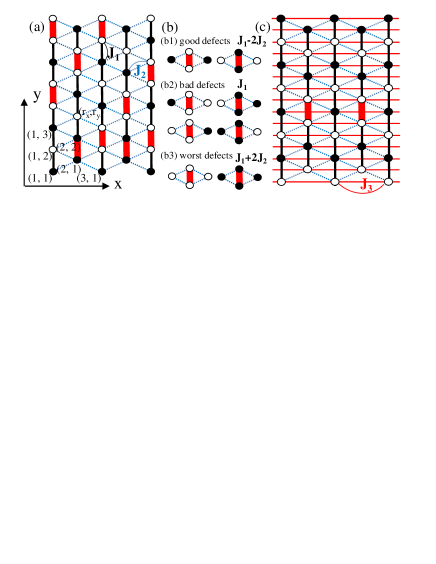
The study of the spatially anisotropic Ising model (1) has a long history Diep2 . Wannier has studied thermodynamic properties of the isotropic model (1) with $J_{1}=J_{2}$, by using transfer matrix method Wannier . He has accurately computed the residual entropy for the macroscopically degenerate ground states, and shown that the internal energy has no singular point as a function of temperature $T$. The zero-temperature critical properties Stephenson ; Blote ; Nienhuis ; Blote2 ; Otsuki and effects of some perturbations Mekata ; Landau ; Takayama ; Slotte ; Fujiki ; Kitatani ; Qian have been studied as well. For $J_{1}>J_{2}>0$, the ground states consist of all of the states where Ising chains along the $y$ direction are independently Néel ordered. In fact, when Néel ordered chains align to the $y$ direction, the inter-chain energy is canceled out. As a result, the ground states are semi-macroscopically degenerate comment2 . Houtappel has examined the general anisotropic case with $J_{1}\neq J_{2}$, and derived the exact expression of the partition function Houtappel . Recently, Hotta, et. al. Hotta ; Hotta2 have studied thermodynamic properties of the model (1) with $J_{2}/J_{1}<1$, by using the exact solution of Ref. Houtappel, and Monte Carlo (MC) simulation. They have confirmed that there is no phase transition in the plane of $T$ and $J_{2}/J_{1}(<1)$. They have pointed out that the low-energy physics of the anisotropic model (1) with $J_{2}/J_{1}<1$ are governed by domain-wall excitations (defects) as shown in Fig. 1(a) and (b). The defects are the ferromagnetic bonds cutting Néel ordered state of each Ising chain, and they are classified into three kinds in the energetic sense, as in Fig. 1(b); Good, bad, and worst defects. In a sufficiently low-temperature regime, bad and worst defects disappear and only good defects survive. The inter-chain coupling $J_{2}$ develops a short-range correlation between defects along the $x$ direction, but it does not induce any phase transition.

These results make us infer that defects form a ordering pattern (crystallization of defects) as in electrons of Wigner crystals if we introduce a small interaction between defects in the anisotropic model (1) with $J_{2}/J_{1}<1$. Following this expectation, we will study the possibility of defect crystallization in this paper. To this end, we introduce an additional ferromagnetic interaction $J_{3}<0$ to the $J_{1}$-$J_{2}$ model (1). The new Hamiltonian is given by

$${\cal H}_{J_{1}-J_{2}-J_{3}} = {\cal H}_{J_{1}-J_{2}}+J_{3}\sum_{\langle\langle{\bm{r}},{\bm{r}^{\prime}}\rangle\rangle_{x}}S_{\bm{r}}S_{\bm{r}^{\prime}}.$$ (2)

The $J_{3}$ term is a next-nearest-neighbor interaction along the $x$ direction and is illustrated in Fig. 1(c). The panel (c) shows that a ferromagnetic $J_{3}$ term plays a role of an attraction between two neighboring good defects.

Numerical analysis.$-$ We will apply the standard heat-bath MC method to the $J_{1}$-$J_{2}$-$J_{3}$ model (2). Both lengths of the $x$ and $y$ directions, $L_{x}$ and $L_{y}$, are set to $L$, and the periodic boundary condition for both directions are imposed. The system size $L$ is increased up to 128. Taking the thermal average, we use $O(10^{7})$ MC samplings. Hereafter, we will set $J_{3}/J_{1}=-0.1$ in the model (2) in order to see effects of a ”small” additional interaction $J_{3}$ on defects of the $J_{1}$-$J_{2}$ model (1).

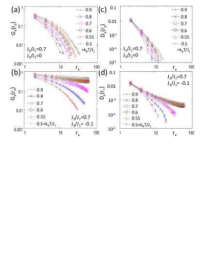
Let us first see temperature $k_{B}T$ and anisotropy $J_{2}/J_{1}$ dependences of spin and defect correlation functions along the $x$ direction. These two correlators are defined as

$$G_{x}(r_{x}) = \langle S_{(1,r_{y})}S_{(r_{x}+1,r_{y})}\rangle-\langle S_{(1,r_{y})}\rangle\langle S_{(r_{x}+1,r_{y})}\rangle,$$ (3)

$$D_{x}(r_{x}) = \langle d_{(1,r_{y})}d_{(r_{x}+1,r_{y})}\rangle-\langle d_{(1,r_{y})}\rangle\langle d_{(r_{x}+1,r_{y})}\rangle.$$ (4)

The quantity $d_{\bm{r}}=(1+S_{\bm{r}}S_{(r_{x},r_{y}+1)})/2$ stands for the defect operator on the bond between $(r_{x},r_{y})$ and $(r_{x},r_{y}+1)$. It takes unity when a defect exists on the bond, while it becomes zero otherwise. Figure 2 shows the $T$ dependence of both spin and defect correlation functions in the models (1) and (2) at $J_{2}/J_{1}=0.7$. The panels (a) and (c) clearly indicates that spin and defect correlation functions decay exponentially irrespective of $k_{B}T$ in the model (1) without $J_{3}$ term. This is consistent with the fact that the $J_{1}$-$J_{2}$ model has no phase transition. On the other hand, panels (b) and (d) show that the decay fashion of spin and defect correlators changes into an algebraic type from an exponential form when $T$ is sufficiently decreased in the $J_{1}$-$J_{2}$-$J_{3}$ model. This power-law behavior strongly suggests the emergence of a quasi long-range order of defects and spins, namely, a Berezinskii-Kosterlitz-Thouless (BKT) phase Berezinskii ; KT ; Kosterlitz ; Kogut ; Kadanoff .

Figure 2: (Color online) (a)(b) Spin correlation functions $G_{x}(r_{x})$ of the models (1) and (2). (c)(d) Defect correlation functions $D_{x}(r_{x})$ of the models (1) and (2). We have set $L=128$ and plotted only the results of even $r_{x}$. The amplitudes of odd $r_{x}$ are very small.

To judge whether or not a BKT phase exists and to correctly determine the BKT transition point from the MC results, we should more carefully treat them rather than those of usual second-order transitions. Here, we utilize the finite-size scaling based on ratios of two spin correlators, that has been developed in Ref. Tomita, . Around a continuous transition or in a BKT phase of the models (1) and (2) with size $L$ (if they exist), a ratio of two spin correlation functions is expected to satisfy the following scaling relation:

$$\frac{G_{x}(r_{x},T,L)}{G_{x}(r_{x}^{\prime},T,L)} = f(L/\xi_{x}),$$ (5)

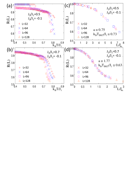
where $f(L/\xi_{x})$ is a function, $\xi_{x}$ is the correlation length of $G_{x}$, and the ratio of two lengths $r_{x}/r_{x}^{\prime}$ is fixed regardless of $T$ and $L$. Here, we have explicitly denoted $T$ and $L$ dependences of $G_{x}$. Since $\xi_{x}$ diverges in a BKT phase, the left-hand side of Eq. (5) becomes independent of the size $L$ there. In Fig. 3(a) and (b), we plot

$$R(L) = \frac{G_{x}(L/2,T,L)}{G_{x}(L/4,T,L)}$$ (6)

as a function of $T$ in the $J_{1}$-$J_{2}$-$J_{3}$ models with different sizes. These two panels uncover that $R(L)$ is almost invariant under changing the size $L$ in a finite temperature range. This strongly suggests that a BKT phase emerges due to the $J_{3}$ term. In the paramagnetic phase near the BKT transition point, $\xi_{x}$ is expected to behave as

$$\xi_{x} \propto \exp(a/\sqrt{t})$$ (7)

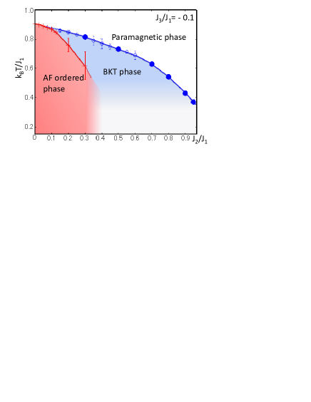
where $a$ is a nonuniversal constant, $t=(T-T_{BKT})/T_{BKT}$, and $T_{BKT}$ is the BKT transition temperature. Therefore, if we plot $R(L)$ as a function of $Le^{-a/\sqrt{t}}$ finely tuning parameters $a$ and $T_{BKT}$, $R(L)$ with different $L$ and $T$ all align on a single curve in the regime $t\ll 1$. Such curves are depicted in Fig. 3(c) and (d). Using this scaling method, we determine $T_{BKT}$ in the wide range of $0<J_{2}/J_{1}<1$ with fixing $J_{3}/J_{1}=-0.1$.

Figure 3: (Color online) (a)(b) Ratio of two spin correlators $R(L)$ as a function of $T$. (c)(d) $R(L)$ as a function of $L/\xi_{x}$ with $\xi_{x}=e^{a/\sqrt{t}}$. Parameters $a$ and $t$ (i.e., $T_{BKT}$) are finely tuned.

These points $T_{BKT}$ are given by filled circles in Fig. 4.

Figure 4: (Color online) Phase diagram of the model ${\cal H}_{J_{1}-J_{2}-J_{3}}$ in the space $(k_{B}T,J_{2})$. Incommensurate ordered phases (see the text) might appear between BKT and AF ordered phases.

From spin and defect correlation functions in Fig. 2, we can also evaluate their critical exponents $\eta_{s}$ and $\eta_{d}$, that are defined as

$$G_{x}(r_{x})\sim r_{x}^{-\eta_{s}}, D_{x}(r_{x})\sim r_{x}^{-\eta_{d}},$$ (8)

where spatially oscillating factors of $G_{x}$ and $D_{x}$ are neglected (We again note that all the plotted positions $r_{x}$ are even in Fig. 2). The evaluated exponents are plotted in Fig. 5.

Figure 5: (Color online) Critical exponents of spin and defect correlation functions (a) $\eta_{\rm s}$ and (b) $\eta_{\rm d}$ at $J_{2}/J_{1}=0.7$, where $k_{B}T_{BKT}/J_{1}\approx 0.63$. In the calculation of $\eta_{s,d}$, we have used the data $G_{x}(r_{x})$ and $D_{x}(r_{x})$ in the range $10<r_{x}<50$ for the $L=128$ systems.

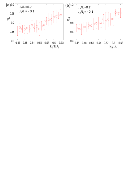
Although there exist large errors in the data of Fig. 5, the result indicates that $\eta_{s}$ ($\eta_{d}$) takes the value $\sim 1/4$ (unity) at $T=T_{BKT}$, and it monotonically decreases with lowering $T$ in the BKT phase. We remark that for the well-studied XY model on a square lattice, the critical exponent of the spin correlation also takes 1/4 at the BKT transition point KT ; Kosterlitz ; Kadanoff . Namely, Ising spins $S_{\bm{r}}$ of the present $J_{1}$-$J_{2}$-$J_{3}$ model exhibit the same asymptotic behavior as XY spins of the XY model in the BKT phase. From this property of $\eta_{s,d}$, we can also determine $T_{BKT}$ as the point where $\eta_{s}=1/4$ ($\eta_{d}=1$). Temperatures $T_{BKT}$ evaluated from $\eta_{s,d}$ are plotted by open circles in Fig. 4. From these results, we conclude that a small $J_{3}$ term causes a BKT phase, and it can be understood as the quasi long-range ordered phase of defects and spins.

In addition to the BKT phase, we also find an AF ordered phase in the $J_{1}$-$J_{2}$-$J_{3}$ model. In fact, at an extreme case with $J_{2}=0$, the system is reduced to two decoupled spatially anisotropic Ising models on square lattice that are exactly solvable and have a second-order phase transition to a Néel phase McCoy . At $J_{2}=0$, the transition temperature $T_{c}$ is exactly calculated as

$$\sinh\left(\frac{2J_{1}}{k_{B}T_{c}}\right)\sinh\left(\frac{2|J_{3}|}{k_{B}T_{c}}\right) = 1,$$ (9)

which leads to $k_{B}T_{c}\approx 0.906J_{1}$ at $J_{3}/J_{1}=-0.1$. The ordering pattern is illustrated in Fig. 6 (c1) and (c2). Hence, their order parameters are respectively defined as $m_{1}=L^{-2}\sum_{r_{x},r_{y}}(-1)^{r_{y}}S_{\bm{r}}$ and $m_{2}=L^{-2}\sum_{r_{x},r_{y}}(-1)^{r_{y}+r_{x}+1}S_{\bm{r}}$. The corresponding susceptibilities are given by

$$\chi_{1,2} = \frac{1}{k_{B}T}\left(\langle m_{1,2}^{2}\rangle-\langle m_{1,2}\rangle^{2}\right).$$ (10)

In Fig. 6(a) and (b), we draw the MC evaluated susceptibility $\chi_{\rm max}={\rm Max}(\chi_{1},\chi_{2})$ as a function of $T$. It exhibits a peak at a certain temperature, and the peak becomes sharper with increasing the system size $L$. We have confirmed that below the temperature showing the peak, an AF order pattern (c1) or (c2) in Fig. 6 appears in the MC snap shots. Since the universality class of this transition is never known, we determine the transition temperature $T_{c}$ through a naive finite-size scaling for the peak of $\chi_{\rm max}$.

Figure 6: (Color online) (a)(b) Susceptibility $\chi_{\rm max}$ for the order parameter of the AF phase. (c1)(c2) AF ordering patterns. (d1)(d2) Examples of possible incommensurate ordering patterns.

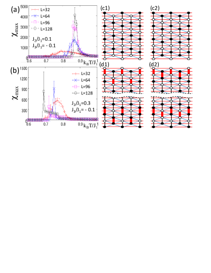
The evaluated $T_{c}$ are depicted in Fig. 4, and one sees from it that $T_{c}$ is lower than $T_{BKT}$ and it monotonically decreases with increasing $J_{2}/J_{1}$. When $J_{2}/J_{1}$ exceeds $\sim 0.4$, the evaluated $T_{c}$ becomes extremely small and the error of the finite-size scaling becomes much larger. Therefore, we cannot determine $T_{c}$ in the range $J_{2}/J_{1}>0.4$. We also see that the peak positions of $\chi_{\rm max}$ seem to irregularly change as a function of $L$. This strange behavior of $\chi_{\rm max}$ and large errors of the finite-size scaling for $T_{c}$ would be related with following things: (i) the MC simulation becomes less reliable in a low-temperature regime due to effects of frustration and defects, and (ii) the BKT phase above $T_{c}$ might largely affect the AF ordered phase when we consider finite-size systems. We will again discuss the nature of the AF transition at $T_{c}$ later. We note that it is difficult to determine whether or not the BKT transition curve starts from the $J_{2}/J_{1}=0$ axis and it coincides with $T_{c}$ at the axis in Fig. 4.

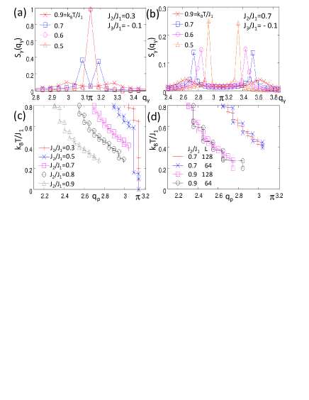
Now, we turn to correlations along the $y$ direction, especially, focusing on the BKT phase. Similarly to Eq. (4), we define the spin correlation function along the $y$ direction $G_{y}(r_{y})=\langle S_{(r_{x},1)}S_{(r_{x},r_{y}+1)}\rangle-\langle S_{(r_{x},1)}\rangle\langle S_{(r_{x},r_{y}+1)}\rangle$. Figure 7(a) and (b) show the spin structure factor for the $y$ direction, that is defined as

$$S_{y}(q_{y}) = \frac{1}{L}\sum_{r_{y}=0}^{L-1}\cos(q_{y}r_{y})G_{y}(r_{y}).$$ (11)

It has a double peak structure around wave number $q_{y}=\pi$. The temperature dependence of one peak position $q_{y}=q_{p}<\pi$ are depicted in Fig. 7(c) and (d). They show that $q_{p}$ monotonically approaches to $\pi$ with lowering $T$ in the whole region $0<J_{2}/J_{1}<1$. This is naturally understood because $q_{p}=\pi$ in the AF ordered phase ($T<T_{c}$), and $q_{p}$ is expected to deviate in proportion to the defect density $\langle d_{\bm{r}}\rangle$ that monotonically grows with increasing $T$. From Fig. 7, we see that $G_{y}$ is incommensurate in the paramagnetic and BKT phases. We have confirmed that the ”commensurate” spin correlator $G_{y}(r_{y})/\cos(q_{p}r_{y})$ exhibits a power-law behavior $\sim r_{y}^{-\eta_{s}}$ in the BKT phase. This is an additional evidence for the existence of the BKT phase. The incommensurate nature of $G_{y}$ also suggests the possibility of single or multiple intermediate phases with an incommensurate order between the BKT and AF ordered phases. Typical order patterns of possible intermediate phases are given in Fig. 6(d1) and (d2), and they are nothing but defect crystals. It is however hard to judge whether or not such phases exist since the MC simulation does not work well in $k_{B}T\ll J_{1}$ and anyone never knows the universality of the phase transition to such intermediate phases.

Figure 7: (Color online) (a)(b) Spin structure factors $S_{y}(q_{y})$. (c)(d) Temperature dependence of a peak position $q_{p}(<\pi)$ of $S_{y}(q_{y})$.

Viewpoints of statistical physics and field theory.$-$ Finally, we discuss the phases and transitions of the $J_{1}$-$J_{2}$-$J_{3}$ model from the viewpoints of field theory and statistical physics. We have uncovered that the $J_{1}$-$J_{2}$-$J_{3}$ model with $J_{3}/J_{1}=-0.1$ has two successive transitions ($T_{BKT}$ and $T_{c}$) with lowering $T$ at least in the range $0.1<J_{2}/J_{1}<0.4$. In addition to the present model, a few two-dimensional (2D) classical systems with a BKT phase in an intermediate-temperature range have been known. $N$-state clock models with $N\geq 5$ are typical example JKKN ; Lecheminant ; Kumano . Usually, in such systems, both the transition between paramagnetic and BKT phases and that between BKT and ordered phases belong to the BKT universality class. Order parameters usually grow very slowly in the BKT class. However, the sharp susceptibility of Fig. 6 implies that the transition at $T_{c}$ is a first- or second-order type. To resolve this discrepancy, we can expect some scenarios. The first scenario is that the behavior of $\chi_{\rm max}$ reduces to a BKT type in the thermodynamic limit. The second is (as we mentioned) the possibility of additional incommensurate phases between BKT and AF phases. If the intermediate-temperature transition is a BKT type, the lowest-temperature one may be first- or second-order. The third is that the transition between the BKT and AF phases is a commensurate-incommensurate (C-IC) type Pokrovsky ; Giamarchi ; Allen . There would also be the possibility that the transition is a first-order type. In general, first-order transitions do not need to obey a usual picture of the renormalization group. The fourth is that the AF order parameter $m_{1,2}$ and the defects are effectively decoupled in the long-distance physics. To determine the true scenario is an interesting future problem. To find the vortex picture of our BKT phase is another important issue. In fact, for the BKT (floating) phase of the 2D anisotropic next-nearest-neighbor Ising (ANNNI) model, the vortex has been defined Allen ; Villain ; Sato ; Rastelli . For the BKT phase of the triangular Ising model with isotropic nearest-neighbor and next-nearest-neighbor couplings Mekata ; Takayama ; Landau , a vortex picture has also been proposed Fujiki .

BKT phases should be generally described by a conformal field theory (CFT) with central charge $c=1$ Yellow ; Giamarchi . The effective action for our BKT phase would be given by

$${\cal A}=\int dxdy\,\,\,\frac{1}{2}(\partial_{\mu}\phi)^{2}+g_{1}\cos(\sqrt{4\pi K}\phi)+\cdots,$$ (12)

where $(x,y)$ is the continuous coordinate stemming from the discrete site $(r_{x},r_{y})$, $\phi$ is a scalar field, and $K$ is the so-called Tomonaga-Luttinger (TL) liquid parameter Giamarchi . In the BKT phase the $g_{1}$ term with scaling dimension $K$ and other perturbations are all irrelevant, and the effective action is given by the Gaussian part $(\partial_{\mu}\phi)^{2}$, while the $g_{1}$ term becomes relevant ($K<2$) in $T>T_{BKT}$ and any quasi long-range correlation disappears. As we mentioned, Fig. 5 indicates that Ising spins play the same role as spins of 2D XY model in the BKT phase. The figure also suggests the relation $\eta_{d}\approx 4\eta_{s}$. From these two results, we can expect the following correspondence between operators of the model (2) and the $c=1$ CFT:

$$S_{\bm{r}}\sim\cos({\sqrt{\pi/K}\theta}), d_{\bm{r}}\sim\cos({2\sqrt{\pi/K}\theta})$$ (13)

where we have neglected spatially oscillating factors. The field $\theta$ is the dual Yellow ; Giamarchi of $\phi$, and $\langle e^{in\sqrt{\pi/K}\theta(r)}e^{-in\sqrt{\pi/K}\theta(0)}\rangle\sim r^{-n^{2}/(2K)}$ in the BKT phase. Since the low-temperature nature around $T=T_{c}$ has not been revealed enough, it is hard to develop the effective theory describing the physics around $T_{c}$. An approach from the $J_{2}/J_{1}=0$ limit might be effective to develop such a field theory Allen . If the transition at $T_{c}$ is a C-IC type, a term $\partial_{y}\phi$ Giamarchi might be necessary in Eq. (12).

Conclusion.$-$ In conclusion, we have studied the spatially anisotropic triangular Ising model (2) with an additional $J_{3}$ term. We have shown that a small $J_{3}<0$ leads to a BKT phase in a wide parameter range and its effective field theory has been proposed. The BKT phase can be regarded as a quasi long-range ordered phase of defects and spins, and an incommensurate spin correlation along the $y$ direction appears there. To develop the vortex picture and to reveal the low-temperature phases are important remaining issues.

Acknowledgment.$-$ We thank Yuta Kumano and Norikazu Todoroki for valuable discussions. This work is supported by KAKENHI (Grant No. 25287088).

References

- (1) See, as a review of triangular antiferromagnets, M. F. Collins and O. A. Petrenko, Can. J. Phys. 75, 605 (1997).
- (2) See, as a review of frustrated quantum magnets, Introduction to Frustrated Magnetism, edited by C. Lacroix, P. Mendels, and F. Mila (Springer-Verlag, Berlin, 2011).
- (3) See, as a review of frustrated magnets, Frustrated Spin Systems, edited by H. T. Diep (World Scientific, Singapore, 2004).
- (4) H. Kawamura, J. Phys.: Cond. Mat. 10, 4707 (1998).
- (5) See, as a review of multiferroics, K. F. Wang, J. -M. Liu, and Z. F. Ren, Advances in Physics 58, 321 (2009).
- (6) See, for example, Chapter 13 of Ref. Lacroix, .
- (7) See, for example, L. Balents, Nature 464, 199 (2010).
- (8) See, for example, Chapters 1 and 2 of Ref. Diep, .
- (9) G. H. Wannier, Phys. Rev. 79, 357 (1950).
- (10) J. Stephenson, J. Math. Phys. 11, 413 (1970).
- (11) H. W. J. Blöte and H. J. Hilborst, J. Phys. A 15, L631 (1982).
- (12) B. Nienhuis, H. J. Hilhorst and H. W. J. Blöte, J. Phys. A 17, 3359 (1984).
- (13) H. W. J. Blöte and M. P. Nightingale, Phys. Rev. B 47, 15046 (1993).
- (14) H. Otsuka, Y. Okabe and K. Okunishi, Phys. Rev. E 73, 035105(R) (2006).
- (15) M. Mekata, J. Phys. Soc. Jpn. 42, 76 (1977).
- (16) D. P. Landau, Phys. Rev. B 27, 5604 (1983).
- (17) H. Takayama, K. Matsumoto, H. Kawahara, and K. Wada, J. Phys. Soc. Jpn. 52, 2888 (1983).
- (18) P. A. Slotte and P. C. Hemmer, J. Phys. C: Solid State Phys., 17, 4645 (1984).
- (19) S. Fujiki, K. Shutoh, and S. Katsura, J. Phys. Soc. Jpn. 53, 1371 (1984).
- (20) H. Kitatani and T. Oguchi, J. Phys. Soc. Jpn. 57, 1344 (1988).
- (21) X. Qian and H. W. J. Blöte, Phys. Rev. E 70, 036112 (2004).
- (22) For , the ground-state residual entropy is proportional to , where is the system size.
- (23) R. M. F. Houtappel, Physica (Amsterdam) 16, 425 (1950).
- (24) C. Hotta, T. Kiyota, and N. Furukawa, Europhys. Lett. 93, 47001 (2011).
- (25) C. Hotta, T. Yoshida, T. Kiyota, and N. Furukawa, private communication.
- (26) V. L. Berezinskii, Sov. Phys. JETP 32, 493 (1971).
- (27) J. M. Kosterlitz and D. J. Thouless, J. Phys. C 6, 1181 (1973).
- (28) J. M. Kosterlitz, J. Phys. C 7, 1046 (1974).
- (29) J. B. Kogut, Rev. Mod. Phys. 51, 659 (1979).
- (30) L. P. Kadanoff, Statistical Physics, (World Scientific, Singapore, 2000).
- (31) Y. Tomita and Y. Okabe, Phys. Rev. B 66, 180401(R) (2002).
- (32) See, for example, B. M. McCoy, Advanced Statistical Mechanics, (Oxford University Press, New York, 2010).
- (33) J. V. José, L. P. Kadanoff, S. Kirkpatrick, and D. R. Nelson, Phys. Rev. B 16, 1217 (1977).
- (34) P. Lecheminant, A. O. Gogolin, A. A. Nersesyan, Nucl. Phys. B 639, 502 (2002).
- (35) Y. Kumano, K. Hukushima, Y. Tomita, and M. Oshikawa, arXiv:1301.6166.
- (36) V. L. Pokrovsky and A. L. Talapov, Phys. Rev. Lett. 42, 65 (1979).
- (37) T. Giamarchi, Quantum Physics in One Dimension, (Oxford University Press, New York, 2004).
- (38) D. Allen, P. Azaria and P. Lecheminant, J. Phys. A: Math. Gen. 34, L305 (2001).
- (39) J. Villain and P. Bak, J. Physique 42, 657 (1981).
- (40) A. Sato and F. Matsubara, Phys. Rev. B 60, 10316 (1999).
- (41) E. Rastelli, S. Regina and A. Tassi, Phys. Rev. B 81, 094425 (2010).
- (42) P. D. Francesco, P. Mathieu and D. Sénéchal, Conformal Field Theory, (Springer-Verlag, New York, 1997).