A Differential Equations Approach to Optimizing Regret Trade-offs

Abstract

We consider the classical question of predicting binary sequences and study the optimal algorithms for obtaining the best possible regret and payoff functions for this problem. The question turns out to be also equivalent to the problem of optimal trade-offs between the regrets of two experts in an “experts problem”, studied before by [14]. While, say, a regret of $\Theta(\sqrt{T})$ is known, we argue that it important to ask what is the provably optimal algorithm for this problem — both because it leads to natural algorithms, as well as because regret is in fact often comparable in magnitude to the final payoffs and hence is a non-negligible term.

In the basic setting, the result essentially follows from a classical result of Cover from ’65. Here instead, we focus on another standard setting, of time-discounted payoffs, where the final “stopping time” is not specified. We exhibit an explicit characterization of the optimal regret for this setting.

To obtain our main result, we show that the optimal payoff functions have to satisfy the Hermite differential equation, and hence are given by the solutions to this equation. It turns out that characterization of the payoff function is qualitatively different from the classical (non-discounted) setting, and, namely, there’s essentially a unique optimal solution.

1 Introduction

Consider the following classical game of predicting a binary $\pm 1$ sequence. The player (predictor) sees a binary sequence $\{b_{t}\}_{t\geq 1}$, one bit at a time, and attempts to predict the next bit $b_{t}$ from the past history $b_{1},\ldots b_{t-1}$. The payoff (score) of the algorithm is then the count of correct guesses minus the number of the wrong guesses, formally defined as follows, for some target time $T>0$, and where $\tilde{b}_{t}$ is the prediction at time $t$:

$$A_{T}=\sum_{1\leq t\leq T}b_{t}\tilde{b}_{t}.$$

One can view this game as an idealized “stock prediction” problem as follows. Each day, the stock price goes up or down by precisely one dollar, and the player bets on this event. If the bet is right, the player wins one dollar, and otherwise she looses one dollar. Not surprisingly, in general, it is impossible to guarantee a positive payoff for all possible scenarios (sequences), even for randomized algorithms. However, one could hope to give some guarantees when the sequence has some additional property.

The above sequence prediction problem is in fact precisely equivalent to the two experts problem (or multi-armed bandits problem), where one considers two experts, via a reduction: one side of the reduction follows simply by using two experts, one always predicts “+1” and another always predicts “-1”. Then one measures the regret of an algorithm: how much worse one’s algorithm does as opposed to the best of the two experts (in hindsight, after seeing the sequence), which is equal to $|\sum_{1\leq t\leq T}b_{t}|$. We will henceforth will refer to $\sum_{1\leq t\leq T}b_{t}$ as the “height” of the sequence (as in the height of a growth chart of a stock). Regret has been studied in a number of papers, including [12, 22, 13, 5, 4]. A classical result says that one can obtain a regret of $\Theta(\sqrt{T})$ for a sequence of length $T$, via, say, the weighted majority algorithm of [22]. Note that the payoff per time step $b_{t}\tilde{b}_{t}$ is essentially equivalent to the well known absolute loss function $|b_{t}-\tilde{b}_{t}|$ (see for example  [10], chapter 8).

Obtaining a regret of $\Theta(\sqrt{T})$ has since become the golden standard for many similar expert learning problem. But is this the best possible guarantee? While there is a lower bound of $\Omega(\sqrt{T})$, it is natural to ask what is the optimal algorithm for minimizing the regret, departing from asymptotic notation. Note that the weighted majority algorithm may not be optimal, even if it obtains the “right order of magnitude”. More generally, one can ask what exactly are all possible payoff functions one can achieve as a function of the total payoffs of the two arms (height, in our case).

In this paper, we undertake precisely this task, of studying the algorithms that obtain the optimal, minimal regret possible and characterize the possible payoff functions. Our results also lead to optimal regret trade-offs between two experts in the experts problem from the equivalence between the two problems. The latter problem has been previously studied by [14], and later by [20], to address, say, an investment scenario where there may be two experts one risk taking and another conservative and one may be willing to take different regrets with respect to these two experts. In particular, it is known that it is possible to get regret $O(\sqrt{T\log T})$ with respect to one expert and $1/T^{\Omega(1)}$ with respect to the other.

There are several reasons to study such optimal algorithms and compute the exact trade-off curves. First of all, such an optimal algorithm may be viewed as more “natural”, for example, because if an autonomous system has the same optimization criteria (of minimizing regret), it would arrive at such an “optimal” solution. Second, it is worthwhile to go beyond the asymptotics of a $\Theta(\sqrt{T})$ bound. Specifically, often the final value of a sequence is actually of the order of $\sqrt{T}$, such as for a random sequence. Although, we do not expect to obtain a positive payoff for a random sequence, a large fraction of all sequences still have $O(\sqrt{T})$ value. In such a scenario, it is critical to obtain the best possible constant in front of the $\sqrt{T}$ regret bound. When the value of the sequence is indeed around $\Theta(\sqrt{T})$, an algorithm with a regret of $\Theta(\sqrt{T})$ achieves a constant factor approximation, and improving the leading constants leads to an approximation factor which is a better constant. For example, in several investment scenarios it is known that the payoffs of the experts (or stocks) in time $T$ is barely more than $O(\sqrt{T})$ (see, for example, the Hurst coefficient measurements of financial markets in [6, 26]). In such settings, the precise constant in regret term can translate into a difference between gain and loss. Indeed, we find that our algorithm can have a regret that is about $10\%$ lower than that of the well known weighted majority algorithm and, at several positions on the curve, our payoff is improved by as much as $0.3\sqrt{T}$ (see figure 1(a)). We also obtain the exact trade-off curve between the regrets with respect to two arms (see figure 2).

We note that, in the vanilla setting, when there is a time bound $T$, the solution already follows from the results of [12] (see also [9, 10]), who gave a characterization of all possible payoffs back in 1965. One can also obtain the optimal algorithm by computing a certain dynamic programming, similar to an approach from [21]. Yet, the resulting algorithm has a betting strategy and payoff function that are time-dependent as well as depend on the final stopping time $T$. These dependencies introduce issues and parameters that are hard to control in reality (often the predictor does not really know when the time “stops”). To understand the time-independent strategies, we are led to consider the another classic setting of time-discounted payoffs (see [17, 27]).

Thus we focus our study on regret-optimal algorithms in the time-discounted setting, where payoff is discounted, and there is no apriori time bound. Formally, we define a $\rho-$discounted version of payoff at some moment of time $T$, for a discount factor $\rho\in(0,1)$, as

$$A_{T}^{\rho}=\sum_{t\geq 0}b_{T-t}\tilde{b}_{T-t}\cdot\rho^{t}$$

The question then is to minimize the regret with respect to this quantity, as a function of (discounted) height. One can also see this scenario as capturing the situation where we care about a certain “attention” window of time (given by $\rho$). One of the consequences of our study is that, when the strategies are time-independent, the characterization of the optimal regret/algorithms becomes quite different.

1.1 Statement of Results

In general, we study the optimal regret curves. Namely, we measure the payoff and regret as a function of the “height” of the sequence (the sum of the bits of the sequence, as defined above; one can also take a discounted sum). Note that comparing against height amounts to comparing the performance of our algorithm against that of two static experts: one that always predicts +1 (“long the stock”), and another that always predicts -1 (“short the stock”). The former obtains a payoff equal to the height and the latter obtains a payoff equal to negative height.

We use the notion of a payoff function — a real function $f$, which assigns algorithm’s payoff $f(x)$ for each height value $x$. In particular, for fixed algorithm and a height $x$, let $f_{T}(x)$ denote the minimum payoff over all sequences with height $x$ at time $T$. For a certain function $f_{T}$, we will say that $f_{T}(x)$ is feasible if there is an algorithm with payoff at least $f_{T}(x)$ over all possible sequences $\{b_{t}\}$ such that $h(\{b_{t}\})=x$. In the discounted scenario, the notion of height becomes the discounted height: $h_{T}^{\rho}(\{b_{t}\}_{t\leq T})=\sum_{t\geq 0}b_{T-t}\rho^{t}$. More importantly, for time-independent strategies (in the discounted setting) we will say that $f(x)$ is feasible if the payoff is at least $f(x)$ for (discounted) height $x$ at all times (feasible in steady state).

Our goal will be to optimize the regret, defined for a payoff function $f$, as follows:

$$R(f)=\max_{x}|x|-f(x),$$

where $x$ ranges over all possible (discounted) heights.

Note that $|x|$ is the maximum of the payoff of the two constant experts. In general, we allow bets $\tilde{b}_{t}$ to be bounded reals in the interval $[-1,1]$. In such a case, it is sufficient to consider deterministic strategies only. One can also consider the version of the problem when there is no restriction on the range of values for $\tilde{b}_{t}$. We will refer to this case as the sequence prediction problem with unbounded bets. This will be useful in deriving bounds for the standard case with bounded bets.

For starters, we remind the result for the vanilla, non-discounted, fixed stopping time setting, which follows from [12], and is related to Rademacher complexity of the predictions of the two experts (see [9, 10]). The theorem below also extends to the discounted scenario, with fixed stopping time $T$. See Appendix A.2 for discussion of this settings.

Theorem 1.1.

Consider the problem of prediction of binary sequence. The minimal possible regret is

$$R=\min_{f}R(f)=\sqrt{\frac{2}{\pi}}\sqrt{T}+O(1).$$

There is a prediction algorithm (betting strategy) achieving this optimal regret and has $f(x)=|x|-R$. The actual corresponding betting strategy may be computing via dynamic programming.

Furthermore, $f$ is feasible iff $\sum f(x)p(x)=0$ where $p(x)$ is the probability of a random walk of length $T$ to end at $x$ (i.e., ${\mathbb{E}\left[f(x)\right]}=0$ for $x$ being the height of a random sequence). For bounded bet value, we have the additional constraint that $f$ is $1$-Lipschitz.

Time-independent strategies.

Our main result is for optimal regret curves in the setting of discounted and time-independent strategies. We characterize the set of all-time feasible $f$’s. For this, we define a certain “optimal” curve function, which will be central to our claims. For constants $c_{1},c_{2}$, define the following function:

$$F_{c_{1},c_{2}}(x)=c_{1}\left(x\cdot\operatorname{erfi}(x)-e^{x^{2}}/\sqrt{\pi}\right)+c_{2}x,$$

where $\operatorname{erfi}(x)=i\cdot\operatorname{erf}(ix)$ is the imaginary error function. We also define $\hat{F}_{c_{1},c_{2}}$ to be the function obtained by bounding the derivative of $F$ to lie in $[-1,1]$. That is $\hat{F}=F$ when $|F^{\prime}|\leq 1$ and $\hat{F}^{\prime}=\text{sign}(F^{\prime})$ when $|F^{\prime}|>1$.

Theorem 1.2 (Main).

Consider the problem of discounted prediction of binary sequence with the discount factor of $\rho=1-1/n$ (corresponding to a “window size” of $n$). A payoff function $f$ is feasible in the steady state if there exist constants $c_{1},c_{2}$ such that for all $x\in[-n,n]$:

$$f(x)\leq\sqrt{n}\cdot\hat{F}_{c_{1},c_{2}}(x/\sqrt{n})-O(1).$$

Conversely, if there exists a function $g$ such that $f(x)=\sqrt{n}\cdot g(x/\sqrt{n})$ for infinitely many $n$ and $g$ is piecewise analytic then $g(x)\leq\hat{F}_{c_{1},c_{2}}(x)$ for some constants $c_{1},c_{2}$.

Hence, the minimum $\rho$-discounted regret is, for $C=\min_{\alpha\geq 1}\tfrac{1}{\sqrt{\pi}}\cdot\tfrac{\alpha}{\operatorname{erfi}(\sqrt{\ln\alpha})}$:

$$\min_{f_{\rho}}R(f_{\rho})=C\sqrt{n}+O(1).$$

We note that the above characterization follows from a “limit view” of the corresponding dynamic programming characterizing the payoff function, which leads to a differential equation formulation of the question. Such an approach has been previously undertaken by [21] to show that many differential equations can be realized as two-person games, as is also the case in our scenario.

In particular, to prove Theorem 1.2, we show that $f$ needs to satisfy the inequality

$$f(x)\geq\frac{f(\rho x+1)+f(\rho x-1)}{2\rho}.$$ (1)

It turns out that, after the correct rescaling, and taking the process to the limit, we obtain a differential equation. Namely, let $g(x)=f(\sqrt{n}x)/\sqrt{n}$ denote a normalized version of $f$ where the axes are scaled down by a factor or $\sqrt{n}$ (the standard deviation of the height). We will assume that $g$ is (piece-wise) analytic. Then, as $n$ approaches infinity, the above inequality implies the following differential inequality:

$$g^{\prime\prime}-2xg^{\prime}+2g\leq 0$$

If we replace the inequality by equality, we obtain the Hermite differential equation which has as its solution the aforementioned functions $F_{c_{1},c_{2}}$. While our solutions are close to these differential equation solutions $F_{c_{1},c_{2}}$, we also point out the curious fact that if we insist on the constraint (1) being an equality, then the only solution is $f(x)=0$. Thus the relaxation into an inequality seems necessary to capture the feasible set of functions.

The algorithm from the above theorem is explicitly given. In particular, it computes the current discounted height $x$, and then outputs the bet $\tilde{b}(x)=\frac{f(\rho x+1)-f(\rho x-1)}{2}$ for the next time step, for $f$ from Theorem 1.2. Surprisingly, the characterization of the feasible payoff functions $f$ is very different when the strategies are time-independent as opposed to the time-dependent case. In particular, in the time-independent case, there are only two degrees of freedom as compared to the time-dependent case when there were infinite (or $\approx n$) degrees of freedom.

See figure 1(a) for the plots of the resulting betting strategy as compared to the one resulting from the multiplicative weights update algorithm (which also happens to be a time-independent strategy). Also, see figure 1(b) for the resulting payoff function $f$ (where the axes have been scaled down by $\sqrt{n}$). After scaling $x$ down by $\sqrt{n}$, we obtain that $\tilde{b}(x)$ tends to $F^{\prime}(x)$ as $n\rightarrow\infty$.

 

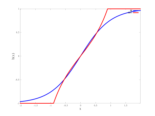
(a) Scaled graphs of the betting strategies for $n=100$ for the weighted majority betting strategy $\tilde{b}(x)=\tanh(x)$ (blue) and the betting strategy resulting from Theorem 1.2, which is equal to $c\operatorname{erfi}(x)$ capped at $\pm 1$ (red). ($x$ axis has been scaled down by $\sqrt{n}$.)

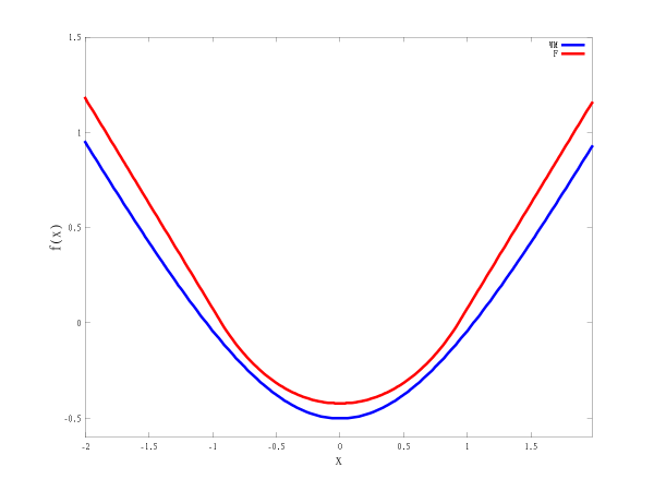
(b) Scaled graphs for the payoff curves $f(x)$, for $n=100$, for the weighted majority algorithm (blue) and the solution resulting from Theorem 1.2 (red). ($x$ and $y$ axes have been scaled down by $\sqrt{n}$.)

Figure 1: Graphs for the prediction of binary sequences problem.

Trading off regrets between two experts.

We also relate our problem to experts problem with two experts (or the multi-armed bandit problem in the full information model with two arms/experts). Here, in each round, each expert has a payoff in the range $[0,1]$ that is unknown to the algorithm. For two experts, let $b_{1,t},b_{2,t}$ denote the payoffs of the two experts at time $t$. The algorithm pulls each arm (expert) with probability $\tilde{b}_{1,t},\tilde{b}_{2,t}\in[0,1]$ respectively where $\tilde{b}_{1,t}+\tilde{b}_{2,t}=1$. The payoff of the algorithm in this setting is $A^{\prime}_{T}:=\sum_{t=1}^{T}b_{1,t}\tilde{b}_{1,t}+b_{2,t}\tilde{b}_{2,t}$. The objective of the algorithm is to obtain low regret with respect to the two experts. We note that this was first studied in  [14].

We achieve the optimal tradeoff between the regrets with respect to the two experts by reducing it to an instance of the sequence prediction problem. In particular, define the loss of a payoff function $f$ as the negative of the minimum value of $f$. Then we show that the regret/loss trade-off for the sequence prediction problem is tightly connected to the trade-off of the regrets with respect to the two experts. Hence, we also derive the regret trade-off for the case of two experts. (See figure 2 for the trade-off curve for the regrets in the two experts problem.)

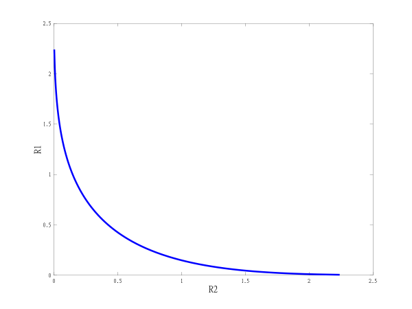
Figure 2: Tradeoff between two regrets $R_{1},R_{2}$ (scaled down by $\sqrt{n}$) for the two experts problem (time-discounted case).

Theorem 1.3.

Consider the problem of trading off regrets $R_{1},R_{2}$ with respect to two experts. Regrets $R_{1},R_{2}$ are achievable in the time-discounted setting if and only if there exists an $\alpha>0$ such that $T(\alpha R_{1}/\sqrt{n})+T(\alpha R_{2}/\sqrt{n})\geq\alpha/\sqrt{\pi}$, where $T(x)=\operatorname{erfi}(\sqrt{\ln x})$ for $x\geq 1$.

Multiple scales.

Finally, we investigate the possible payoff functions at multiple time scales $\rho$ (window sizes). Several earlier papers considered regrets at different time scales; see [8, 16, 18, 29, 20]. We consider two different time scales, $\rho_{1}=1-1/n_{1}$ and $\rho_{2}=1-1/n_{2}$, although a similar result can be obtained for a larger number of time scales.

We exhibit the necessary and sufficient condition for a feasible payoff function, as window size goes to infinity. In particular, suppose that $n_{1}=a_{1}n$ and $n_{2}=a_{2}n$ where $n$ tends to infinity. Let $x_{1}$ and $x_{2}$ be the time discounted heights for the two different time scales. We can ask if it is possible to get (time discounted) payoff functions $f_{1}(x_{1},x_{2})$ and $f_{2}(x_{1},x_{2})$ at time scales $n_{1}$ and $n_{2}$ respectively. Again we apply the coordinate rescaling by $\sqrt{n}$ for both $x_{1},f_{1}$ and $x_{2},f_{2}$.

Theorem 1.4.

For $n\geq 1$, fix two windows $n_{1}=a_{1}n$ and $n_{2}=a_{2}n$. As $n$ goes to infinity, there is are payoff function $f_{1}(x_{1},x_{2})=\sqrt{n}g_{1}(x_{1}/\sqrt{n},x_{2}/\sqrt{n})$ for the discount rate $\rho_{1}=1-1/n_{1}$ and $f_{2}(x_{1},x_{2})=\sqrt{n}g_{2}(x_{1}/\sqrt{n},x_{2}/\sqrt{n})$ for the discount rate $\rho_{2}=1-1/n_{2}$, as $n$ goes to infinity, if and only if the following system of partial differential inequalities is satisfied:
$E_{1}\triangleq-\frac{1}{2}\left(\frac{\partial}{\partial x_{1}}+\frac{\partial}{\partial x_{2}}\right)^{2}g_{1}+\left(a_{1}^{2}x_{1}\frac{\partial}{\partial x_{1}}+a_{2}^{2}x_{2}\frac{\partial}{\partial x_{2}}\right)g_{1}-a_{1}^{2}\cdot g_{1}\geq 0$
$E_{2}\triangleq-\frac{1}{2}\left(\frac{\partial}{\partial x_{1}}+\frac{\partial}{\partial x_{2}}\right)^{2}g_{2}+\left(a_{1}^{2}x_{1}\frac{\partial}{\partial x_{1}}+a_{2}^{2}x_{2}\frac{\partial}{\partial x_{2}}\right)g_{2}-a_{2}^{2}\cdot g_{2}\geq 0$
$E_{1}+E_{2}\geq\left|\left(\frac{\partial}{\partial x_{1}}+\frac{\partial}{\partial x_{2}}\right)(g_{1}-g_{2})\right|.$

We do not seem to have explicit analytical solution for the above system of inequations, and so perhaps one would have to rely on numerical simulations to solve it. This part is deferred to Appendix C due to space limitation.

1.2 Related Work

There is a large body on work on regret style analysis for prediction. Numerous works including  [12, 9] have examined the optimal amount of regret achievable with respect to multiple experts. Many of the results in this body of work can be found in  [10]. It is well known that in the case of static experts, the optimal regret is exactly equal to the Rademacher complexity of the predictions of the experts (chapter 8 in  [10]). Recent works, including  [1, 2, 23], have extended this analysis to other settings. Measures other than the standard regret measure have been studied in [25]. Also related is the NormalHedge algorithm [11], though it differs in both the setting and the precise algorithm. Namely, NormalHedge looks at undiscounted payoffs and obtains strong regret guarantees to the epsilon-quantile of best experts. We look at two experts case (where epsilon-quantile is not applicable) and seek to obtain provably optimal regret.

Algorithms with performance guarantees within each interval have been studied in [8, 16, 29] and, more recently, in [18, 20]. The question of what can be achieved if one would like to have a significantly better guarantee with respect to a fixed arm or a distribution on arms was asked before in [14, 20]. Tradeoffs between regret and loss were also examined in [28], where the author studied the set of values of $a,b$ for which an algorithm can have payoff $aOPT+b\log N$, where $OPT$ is the payoff of the best arm and $a,b$ are constants. The problem of bit prediction was also considered in [15], where several loss functions are considered. Numerous papers ([7, 19, 3]) have implemented algorithms inspired from regret syle analysis and applied it on financial and other types of data.

2 Time-Independent Prediction Algorithms

In this section we study the optimal regret and algorithms for the time-independent strategies and regret curves. We consider the time-discounted setting, thereby proving Theorem 1.2.

As mentioned in the introduction, we consider a payoff $f$ to be feasible if there is a prediction algorithm that achieves a payoff of at least $f(x)$ for the discounted height $x$ at all times $t\geq 1$. We will argue that, without loss of generality, we can assume that the betting strategy $\tilde{b}(x)$ is time independent and the payoff always dominates the function $f(x)$.

Observe that for a time independent betting function, the payoff function it achieves is also time independent in the limit.

Claim 2.1.

If $f$ is feasible (in steady state), then there is a time-independent betting strategy $\tilde{b}$ that achieves payoff function $f$.

Proof of Claim 2.1.

Remember that we use discount factor of $\rho=1-1/n$, where $n\geq 1$ is the “window” size. Assume there is a time-dependent betting strategy $\tilde{b}_{t}(x)$ that achieves payoff at least $f(x)$ in the steady state. We consider the average of these betting strategies over a long interval and argue that it changes only slightly over time. Note that the time shifted strategy $\tilde{b}_{t-i}$ also achieves payoff at least $f(x)$ at all times. This means that an average of a large number of such shifted betting strategies also achieves this. Consider the average strategy $\mu_{t}(x)=\frac{1}{N}\sum_{i=1}^{N}\tilde{b}_{t-i}(x)$, and note it is essentially constant over a small window for a sufficienly large $N$. For example, if we choose $N>\exp(n)$ the differences in $\mu_{t}$ over a window of size $\operatorname{poly}(n)$ are exponentially small. Since we are time discounting at rate $1-1/n$, it suffices to ignore anything outside such a window of size $\operatorname{poly}(n)$. ∎

We will characterize the payoff functions that are feasible for time-independent betting strategies.

Lemma 2.2.

If there is a time-independent betting strategy with payoff function $f(x)$ then

$$f(x)\geq\frac{f(\rho x+1)+f(\rho x-1)}{2\rho}.$$ (2)

Conversely if $f$ satisfies the above inequality and $f(0)\leq 0$, then it is feasible with unbounded bets. In particular the betting strategy $\tilde{b}(x)=\frac{f(\rho x+1)-f(\rho x-1)}{2}$ achieves a payoff function at least $f$. For the bounded bets case, we need the additional constraint that $\tilde{b}(x)$ computed thus satisfies $|\tilde{b}(x)|\leq 1$

Proof.

Note that since the payoff at time $t$ is $\tilde{b}(x_{t})b$ (where $b=b_{t}$), we have $\rho f(x)+b\tilde{b}(x)\geq f(\rho x+b)$ where $b\in\{\pm 1\}$. This is because at time $t-1$ there is some sequence of height $x$ with payoff $f(x)$. Thus, we have $\rho f(x)+\tilde{b}(x)\geq f(\rho x+1)$ and, similarly, $\rho f(x)-\tilde{b}(x)\geq f(\rho x-1)$. Averaging the two we get inequality (2).

To prove the converse we can use induction on time $t$ to show that the stated betting strategy achieves payoff at least $f(x)$. Clearly at $t=0$, $x=0$ and since $f(0)\leq 0$ the condition is satisfied. Further, if the height is $x$ at time $t-1$ then at the next step the payoff is at least $\rho f(x)+b\tilde{b}(x)\geq f(\rho x+b)$ for $b\in\{-1,1\}$ which follows from the inequality (2). ∎

We now proceed to proving the main claims of Theorem 1.2. In particular, we start by showing the “converse” direction. For this, we will show that, in the limit, the payoff function has to satisfy a certain differential equation, when property scaled. The next lemma proves precisely this switch.

Lemma 2.3.

Let $g(x)=f(\sqrt{n}x)/\sqrt{n}$, and assume it is piece-wise analytic. Then as $n\rightarrow\infty$, condition  (2) becomes

$$g^{\prime\prime}-2xg^{\prime}+2g\leq 0.$$ (3)

Proof.

Rescaling and setting $\delta=1/\sqrt{n}$ (i.e., $\rho=1-\delta^{2}$) in inequality (2) gives us:

$$(1-\delta^{2})g(x)\geq\frac{g((1-\delta^{2})x+\delta)+g((1-\delta^{2})x-\delta)}{2}.$$

Using Taylor expansion on $g$, we obtain

$$(1-\delta^{2})g(x)\geq g(x)-\delta^{2}xg^{\prime}(x)+(1/2)\delta^{2}(1+\delta^{2}x^{2})g^{\prime\prime}(x)+O(\delta^{3})g^{\prime\prime\prime}(x-\delta^{2}x\pm\delta)$$

$$0\geq g(x)-xg^{\prime}(x)+(1/2)(1+\delta^{2}x^{2})g^{\prime\prime}(x)+O(\delta)g^{\prime\prime\prime}(x-\delta^{2}x\pm\delta)$$

As $\delta=1/\sqrt{n}\rightarrow 0$, we obtain that $g^{\prime\prime}-2xg^{\prime}+2g\leq 0$. ∎

We note that if we replace the inequality (2) with the equality, we obtain the Hermite differential equation:

$$g^{\prime\prime}-2xg^{\prime}+2g=0.$$ (4)

Differential equation (4) has a general solution of the form $F_{c_{1},c_{2}}=c_{1}(x\operatorname{erfi}(x)-e^{x^{2}}/\sqrt{\pi})+c_{2}x$, where $\operatorname{erfi}(x)=i\cdot\operatorname{erf}(ix)$ is the imaginary error function.

Remark 2.4.

Note that, for example, this “limiting payoff function” $F_{c_{1},c_{2}}$ satisfies the “limiting” $T\rightarrow\infty$ characterization similar to Theorem A.3. Namely, for any constants $c_{1},c_{2}$, we have that $\int p_{\rho}(x)F_{c_{1},c_{2}}(x)\operatorname{dx}=0$, where $p_{\rho}(x)$ is the distribution of the $\rho$-decayed random walk to be at height $\sqrt{n}x$, at the limit of $n,T\rightarrow\infty$. (Note that $p_{\rho}$ converges to $N(0,1)$ when $n\rightarrow\infty$.)

In the following, we show that the solutions for the steady-state payoffs are essentially characterized by functions $F_{c_{1},c_{2}}$. Note that we thus obtain solutions that have only two degrees of freedom. This is in stark contrast to the time-dependent strategies, where there is an infinite number of degrees of freedom (see Appendix A).

The next lemma shows that if $g(x)=f(\sqrt{n}x)/\sqrt{n}$ satisfies the differential inequality, then $g$ must be dominated by $F_{c_{1},c_{2}}$, i.e., a solution to the Hermite differential equation.

Lemma 2.5.

Suppose $g$ satisfies $g^{\prime\prime}-2xg^{\prime}+2g\leq 0$. Then there exist some $c_{1},c_{2}$, such that $g\leq F_{c_{1},c_{2}}$.

Proof.

There is a unique solution $y=F_{c_{1},c_{2}}$ such that $y(0)=g(0)$ and $y^{\prime}(0)=g^{\prime}(0)$. Now look at $h=g-y$. We will show that $h\leq 0$. Observe that $h$ satisfies $h^{\prime\prime}-2xh^{\prime}+2h\leq 0$ and $h(0)=h^{\prime}(0)=0$.

We will make the substitution $u=xh^{\prime}-h$. Hence we have that $u^{\prime}=xh^{\prime\prime}$, and thus $u^{\prime}/x-2u\leq 0$. or $u^{\prime}\leq 2ux$ for $x\geq 0$ and $u^{\prime}\geq 2ux$ for $x\leq 0$ and $u(0)=0$. This implies that $u\leq 0$. This means that $xh^{\prime}-h\leq 0$ which implies $h\leq 0$. ∎

So far we have ignored the condition that the $|b|\leq 1$ thus allowing unbounded bets. In the following claim, we consider the case of bounded bets and show that in this case the function $g$ has a bounded derivative.

Claim 2.6.

With bounded bets $|b|\leq 1$, the function $g$ must also satisfy the constraint $|g^{\prime}(x)|\leq 1$ as $n\rightarrow\infty$.

Proof.

For $\delta=1/\sqrt{n}$, we have that

$$(1-\delta^{2})g(x)+\delta\geq g((1-\delta^{2})x+\delta)\implies-\delta g(x)+1\geq\frac{g((1-\delta^{2})x+\delta)-g(x)}{\delta}$$

Considering $\delta\rightarrow 0$ gives $g^{\prime}(x)\leq 1$. Similarly we get $-g^{\prime}(x)\leq 1$. ∎

Suppose we choose a solution $g=F_{c_{1},c_{2}}$, this would correspond to the betting strategy $b(x)=c_{1}\cdot\operatorname{erfi}(x)+c_{2}$. Note that $F$ doesn’t satisfy $|g^{\prime}(x)|\leq 1$, but a simple capping of its growth when $|F^{\prime}|\geq 1$ gives a alternate function $\hat{F}$ (see figure 1(b)) that satisfies the extra condition. This essentially corresponds to capping $b(x)$ so that $|b(x)|\leq 1$. Let $\hat{b}(x)$ denote the capped version of $b(x)$ that can be used for bounded bets.

This concludes the “converse” part of Theorem 1.2. Next, we switch to showing the forward direction, that if (a properly scaled) $f$ is dominated by $F$, then it is also a valid payoff function. In particular, in the next lemma, we show that the solutions to the differential inequality can be made to satisfy the original recursive inequality (2) with a small error term.

Lemma 2.7.

For any constants $c_{1},c_{2}$, for the bounded bets case, there is a function $\hat{g}(x)=\hat{F}(x)-O(1/\sqrt{n})$ such that $\sqrt{n}\cdot\hat{g}(\sqrt{n}x)$ satisfies the inequality (2).

With unbounded bets, there is a function $g(x)=F(x)\cdot e^{-O(x^{2}/n+1/n)}$ such that $\sqrt{n}g(\sqrt{n}x)$ satisfies the inequality (2).

Proof.

Let $\delta=1/\sqrt{n}$. We will argue that the $O(\delta)$ slack is sufficient to account for the error in the Taylor approximation in the bounded bets case. To see this note that the error in the Taylor approximation is $\delta^{2}x^{2}g^{\prime\prime}(x)+O(\delta)\bar{g}^{\prime\prime\prime}((1-\delta^{2})x\pm\delta)$, where $\bar{g}^{\prime\prime\prime}(x\pm\epsilon)$ denotes the average of $g^{\prime\prime\prime}$ at two points in the range $x\pm\epsilon$. We will look at the interval where $|F^{\prime}(x)|\leq 1$. For constant $c_{1},c_{2}$ the end points of this interval are also constants which implies all the terms in the error expression are constants (since $f$ is independent of $\delta$). Thus the error is at most $O(\delta)$. So it suffices to satisfy the condition $g^{\prime\prime}-2xg^{\prime}+2g<-O(\delta)$ which is satisfied by $F-O(\delta)$. For the region where $|F^{\prime}(x)|\geq 1$, note that in $\hat{F}$ we are capping $|\hat{F}^{\prime}(x)|=1$ and since $\hat{g}$ is $\hat{F}$ shifted down, it also satisfies the inequality.

For the case of unbounded bets, observe that the recursive inequality holds if we satisfy the following, per the approximation of the Taylor series:

$$\bar{g}^{\prime\prime}(x-x^{2}\delta^{2}\pm\delta)(1+x^{2}\delta^{2})-2xg^{\prime}(x)+2g(x)\leq 0.$$

For simplicity of explanation, consider $x\geq 0$. Note that $\delta x\leq 1$. We have $F^{\prime\prime}(x)=c_{1}e^{x^{2}}$. Suppose we look for a function $g$ that satisfies: $g^{\prime\prime}(x)$ is even and is increasing in $x$ when $x\geq 0$ and $g^{\prime\prime}(x\pm\epsilon)\leq g^{\prime\prime}(x)/e^{4(x^{2}\epsilon^{2}+\epsilon^{2})}$ for a big enough constant in the $O$ — we will later verify that our resulting $g$ indeed satisfies this (note that this is satisfied for $F$). Then, since $(1+x^{2}\delta^{2})\leq e^{O(x^{2}\delta^{2})}$, the above inequality is satisfied as along as

$$g^{\prime\prime}(x)\leq e^{-O(x^{2}\delta^{2}+\delta^{2})}2(xg^{\prime}(x)-g(x))$$

Again, for $u=xg^{\prime}-g$, we get: $\tfrac{u^{\prime}}{x}\leq e^{-O(x^{2}\delta^{2}+\delta^{2})}2u$ which holds if $u\leq e^{x^{2}-O(\delta^{2}+\delta^{2})}$.

So it suffices that $xg^{\prime}-g=e^{x^{2}-O(x^{2}\delta^{2}+\delta^{2})}$. Dividing by $x^{2}$, we get: $(g/x)^{\prime}=e^{x^{2}-O(x^{2}\delta^{2}+\delta^{2})}/x^{2}$. Note that without the correction terms the earlier differential equation $(g/x)^{\prime}=e^{x^{2}}/x^{2}$ has the solution $g=F$, and so for the new equation there is a solution $g=Fe^{-O(x^{2}\delta^{2}+\delta^{2})}$. Note that this $g$ also satisfies $g^{\prime\prime}(x\pm\epsilon)\leq g^{\prime\prime}(x)/e^{4(x^{2}\epsilon^{2}+\epsilon^{2})}$ that we had assumed. ∎

Our Theorem 1.2 is hence concluded by Lemma 2.2 and Lemma 2.7. In the following we remark that obtaining a (non-trivial) solution that preserves the equation (4) precisely is impossible.

Remark 2.8.

If we convert the condition (2) into an equality then the only satisfying analytic solution $f$ is $f(x)=cx$ for a constant $c$. Thus the relaxation into an inequality seems to be necessary to find all the feasible payoff functions

Proof.

If we require the equality $f(x)=\frac{f(\rho x+1)+f(\rho x-1)}{2\rho}$ then applying this recursively $i$ times gives:

$$f(x)=\rho^{-i}\frac{\sum_{b_{1},\cdots b_{i}\in\{-1,1\}}f(\rho^{i}x+\rho^{i-1}b_{1}+\rho^{i-2}\cdots+b_{i})}{2^{i}}$$

We apply Taylor series to $f(\rho^{i}x+\rho^{i-1}b_{1}+\cdots+b_{i})$ around the point $y=\rho^{i-1}b_{1}+\cdots+b_{i}$ to conclude that $f(y+\rho^{i}x)=f(y)+\rho^{i}xf^{\prime}(y)+\rho^{2i}x^{2}f^{\prime\prime}(y\pm\rho^{i}x)$. We now consider the following difference

$$f(x)-f(0)=\rho^{-i}\frac{\sum_{b_{1},\cdots b_{i}\in\{-1,1\}}f(\rho^{i}x+\rho^{i-1}b_{1}+\cdots+b_{i})-f(\rho^{i-1}b_{1}+\cdots+b_{i})}{2^{i}}$$

and using the above expansion, we have

$$f(x)-f(0)=\frac{\sum_{b_{1},\cdots b_{i}\in\{-1,1\},y=\rho^{i-1}b_{1}+\cdots+b_{i}}xf^{\prime}(y)+\rho^{i}x^{2}f^{\prime\prime}(y\pm\rho^{i}x)}{2^{i}}.$$

Taking $i$ tend to infinity, we conclude that $f(x)-f(0)=x\cdot\int p_{\rho}(y)f(y)\operatorname{dy}$. This implies that $f$ is of the form $f(x)=cx+a$. Moreover substituting $f$ into the equality condition, we obtain that $a=0$. ∎

Appendix A Prediction Algorithms for Fixed Stopping Time

In this section we discuss the optimal regret and the corresponding betting algorithm for a fixed stopping time $T$, which leads to strategies that depend on current time $t$ and the stopping time $T$. We consider the classical non-discounted setting (Theorem 1.1) and the time-discounted setting (Theorem A.3), both with fixed stopping time.

In the non-discounted setting, we show that the optimal regret and algorithm follow easily from the existing work of [12].

We note that the resulting prediction algorithms depend on the current time $t$ and the stopping time $T$. We will consider the admittedly more interesting case — of time-independent strategies — in the next section.

A.1 Non-discounted setting

[12] gave a precise characterization of possible payoff curves attainable. First of all, he showed that, if, for a sequence ${\bar{b}}\in\{\pm 1\}^{T}$, we denote $g({\bar{b}})$ to be the payoff/score obtained for sequence ${\bar{b}}$, then $\sum_{\bar{b}}g({\bar{b}})=0$ for all possible algorithms. Cover proves the following characterization of the curve as a function of the height of the sequence:

Theorem A.1 ([12]).

Let $f:{\mathbb{N}}\to{\mathbb{R}}$ be the payoff function of an algorithm, where $f(x)$ is the payoff of an algorithm for sequences of height $x$ precisely. Then $f$ is feasible if and only if: 1) $\sum_{x=0}^{T}{T\choose x}f(T-2x)=0$ and 2) $|f(x+1)-f(x)|\leq 1$ ($f$ is Lipschitz).

From the above theorem we have the following corollary.

Corollary A.2.

$f(x)=|x|-R$ is feasible for $R=\sqrt{2\over\pi}\sqrt{T}+O(1)$, and this is the minimum $R$ for which this is feasible.

Proof.

Note that Theorem A.1 holds for the payoff function $f(x)=|x|-R$, where $R={\mathbb{E}_{{\bar{b}}\in\{\pm 1\}^{T}}\left[|\sum_{i}{\bar{b}}_{i}|\right]}$. To compute this value $R$, we use following standard approximation: $\left|{\mathbb{E}_{{\bar{b}}\in\{\pm 1\}^{T}}\left[|\sum_{i}{\bar{b}}_{i}|\right]}-{\mathbb{E}_{x\sim\phi}\left[|\sqrt{T}x|\right]}\right|\leq O(1)$, where $\phi(x)$ is the normal distribution (see, e.g., [24], Theorem 3.4). Furthermore, we have that ${\mathbb{E}_{x\sim\phi}\left[|\sqrt{T}x|\right]}=\sqrt{2\over\pi}\sqrt{T}$. The corollary follows. ∎

To recover the actual prediction algorithm, we employ the following standard dynamic programming. Namely, define $s_{t}(x)$ to be the minimal necessary algorithm payoff, after $t^{th}$ time step for height $x$, in order to obtain payoffs of $s_{T}(y)=f(y)=|y|-R$. In particular, if $\tilde{b}_{t}(x)$ denotes the prediction (bet) at time $t$ assuming the current height is $x$, we have that $s_{t}(x)=\min_{|b_{t}(x)|\leq 1}\max\{s_{t+1}(x+1)-\tilde{b}_{t+1}(x),s_{t+1}(x-1)+\tilde{b}_{t+1}(x)\}$. Suppose we ignore the boundedness of $b_{t}(x)$, then the minimum is achieved for $b_{t+1}(x)=\tfrac{1}{2}(s_{t+1}(x+1)-s_{t+1}(x-1))$. Note that this way we obtain $s_{0}(0)={\mathbb{E}_{{\bar{b}}\in\{\pm 1\}^{T}}\left[f(\sum_{i}{\bar{b}}_{i})\right]}=0$ (which gives a different proof of the above theorem). But these values of $\tilde{b}$ actually satisfy $|\tilde{b}_{t}(x)|\leq 1$, since if the Lipschitz condition holds at time $t$, then it also holds at time $t-1$. Hence there was no loss of generality of dropping the boundedness of $\tilde{b}_{t}(x)$’s. In particular, we have that $\tilde{b}_{t}(x)=\tfrac{1}{2^{T-t+1}}\sum_{{\bar{b}}\in\{\pm 1\}^{T-t+1}}\left(|x+1+\sum_{j}{\bar{b}}_{j}|-|x-1+\sum_{j}{\bar{b}}_{j}|\right)$.

This concludes the proof of Theorem 1.1 to show the optimal regret and prediction algorithm for the vanilla fixed stopping time setting. Note that the prediction algorithm $\tilde{b}_{t}(x)$ depends on the current time: for example, for $t$ close to $T$ the all bet values are close to 1, whereas for small $t$’s we obtain very small values of $\tilde{b}_{t}(x)$.

A.2 Time-discounted setting

We prove the following theorem for the time-discounted setting with fixed stopping time $T$, by extending the characterization given in Section A.1.

Theorem A.3.

Consider the problem of time-discounted prediction of binary sequence for “window size” $n$. Fix the discount factor $\rho=1-1/n$. For any fixed time $T$, $f_{T}$ is feasible iff $\int f(x)p_{T}(x)\operatorname{dx}=0$ where $p_{T}(x)$ is the probability of a (decayed) random walk to end at height $x$ and $f$ is $1$-Lipshitz (for bounded bet value).

There is an algorithm (betting strategy) achieving this optimal regret and has $f(x)=|x|-R_{\rho}$, where $R_{\rho}=\min_{f}R_{T}(f)=\sqrt{\frac{2}{\pi}}\sqrt{\alpha}+O(1)$, and $\alpha=\tfrac{1-\rho^{2T}}{1-\rho^{2}}$. Note that $\alpha\rightarrow T$ when $T\ll n$, and $\alpha\rightarrow n/2$ when $T\gg n$. The betting strategy may be computing via dynamic programming.

First, we need to count the number of random walks achieving a certain discounted height $x$. When the height was not discounted, this was simply a binomial distribution, which we approximated by a normal distribution. It turns out that, in the discounted height case, the height distribution is also approaches normal distribution at the limit. Specifically, we show the following lemma.

Lemma A.4.

Consider the time-discounted setting, with discount $\rho=1-1/n$ for some $n\geq 1$. Let $p_{T}(x)$ be the probability that a random binary sequence of length $T$ has discounted height $x\in[-n,n]$. Then, as $T$ goes to infinity, the probability distribution of the discounted height, scaled down by $\sqrt{\alpha}$, converges to the normal distribution $N(0,1)$, where $\alpha=\tfrac{1-\rho^{2T}}{1-\rho^{2}}$.

Furthermore, ${\mathbb{E}_{{\bar{b}}\in\{\pm 1\}^{T}}\left[|\sum_{i\geq 1}{\bar{b}}_{i}\rho^{T-i}|\right]}=\sqrt{2\over\pi}\sqrt{\alpha}\pm O(1)$.

Proof.

Note that the height is distributed as $x=\sum_{i=1}^{T}{\bar{b}}_{i}\rho^{T-i}$ where ${\bar{b}}_{i}$ are random $\pm 1$. Then, by Lyapunov central limit theorem, we have that $\tfrac{1}{\sqrt{\alpha}}\sum_{i=1}^{T}{\bar{b}}_{i}\rho^{T-i}$ tends to $N(0,1)$ as long as $T=\omega_{n}(1)$.

Again, we have that (see, e.g., [24], Theorem 3.4) $\left|{\mathbb{E}_{{\bar{b}}\in\{\pm 1\}^{T}}\left[|\sum_{i\geq 1}{\bar{b}}_{i}\rho^{T-i}|\right]}-{\mathbb{E}_{x\sim\phi}\left[|\sqrt{\alpha}\cdot x|\right]}\right|=O(\alpha^{-1})\cdot\sum_{i=0}^{T}\rho^{3i}=O(1).$ Hence, we obtain that ${\mathbb{E}_{{\bar{b}}\in\{\pm 1\}^{T}}\left[|\sum_{i\geq 1}{\bar{b}}_{i}\rho^{T-i}|\right]}=\sqrt{2\over\pi}\sqrt{\alpha}\pm O(1)$. ∎

The rest of the proof of Theorem A.3 follows along the same lines of Theorem 1.1. Specifically, one can employ the same dynamic programming (for all possible discounted heights). We again have that $s_{0}(0)={\mathbb{E}_{x\sim p_{T}}\left[f(x)\right]}$ for any desired target function $f$. The only way $s_{0}(0)=0$ is when ${\mathbb{E}_{x\sim p_{T}}\left[f(x)\right]}=0$. As long as $f$ is also Lipschitz, the dynamic programming will recover the betting strategy with bounded bets $|\tilde{b}_{t}(x)|\leq 1$. As in the previous setting, note that the betting strategy $\tilde{b}_{t}$ depends on the time $t$: it is small at the beginning, and gets closer to 1 for large values of $t$ (close to $T$).

Appendix B Trade-off with two experts

In this section we will prove Theorem 1.3 by proving an equivalence between the sequence prediction problem and the two-experts problem. In each round of the experts problem, each expert has a payoff in the range $[0,1]$ that is unknown to the algorithm. For two experts, let $b_{1,t},b_{2,t}$ denote the payoffs of the two experts. The algorithm pulls the each arm (expert) with probability $\tilde{b}_{1,t},\tilde{b}_{2,t}\in[0,1]$ respectively where $\tilde{b}_{1,t}+\tilde{b}_{2,t}=1$. The payoff of the algorithm is $A=\sum_{t=1}^{T}b_{1,t}\tilde{b}_{1,t}+b_{2,t}\tilde{b}_{2,t}$. Let $X_{1}=\sum_{t=1}^{T}b_{1,t}$ We will study the regret trade-off $R_{1},R_{2}$ with respect to these two experts which means that $A\geq X_{1}-R_{1}$ and $A\geq X_{2}-R_{2}$.

For this we we translate it into an instance of the sequence prediction problem where we show how we can obtain a tradeoff between regret $R$ and loss $L$, which is defined as the minumum payoff of the algorithm. With two experts, the regret/loss tradeoff in the sequence prediction problem is related to regret trade-off for the two experts problem. Let $R$, $L$ be feasible upper bounds on the regret and loss in the sequence prediction problem in the worst case; Let $R_{o},L_{o}$ be feasible upper bounds on the regret and loss with version of the sequence prediction problem with one sided bets (that is $\tilde{b}_{t}$ cannot be negative; the feasible payoff curves for this case is a simple variant of $F_{c_{1},c_{2}}$ where $F^{\prime}$ is capped to lie in $[0,1]$.) Let $R_{1}$, $R_{2}$ be feasible upper bounds in regret with respect to expert one and expert two in the worst case. Another variant that has been asked before is a tradeoff between regret to the average and regret to the max (see [14, 20]). Let $R_{m}$, $R_{a}$ be feasible upper bounds on the regret to the max and regret to the average with two experts in the worst case.

Theorem 1.3 follows from the following two lemmas.

Lemma B.1.

Regret and loss $R,L$ is feasible in the sequence prediction problem if and only if $R_{m}=R/2,R_{a}=L/2$ is feasible for regret to the max and regret to the average in the two experts problem.

$R_{o},L_{o}$ is feasible in the sequence prediction problem (with one sided bets) if and only if $R_{1}=L_{o},R_{2}=R_{o}$ is feasible for regret to the first expert and regret to the second expert in the two experts setting.

For $x\geq 0$, let $T(x)=h(g^{-1}(x))$ where $g(x)=e^{x^{2}},h(x)=\operatorname{erfi}(x)$. Note that $T(x)=\operatorname{erfi}(\sqrt{\ln x})$.

Proof of Lemma B.1.

First we look at reduction from the regret to the average and regret to the max problem. We can reduce this problem to our sequence prediction problem by producing at time $t$, $b_{t}=(b_{1,t}-b_{2,t})/2$. A bet $\tilde{b}_{t}$ in our sequence prediction problem can be translated back into probabilities $\tilde{b}_{1,t}=(1+\tilde{b}_{t})/2$ and $(1-\tilde{b}_{t})/2$ for the two experts. A payoff $A$ in the original problem gets translated into payoff $\sum_{t}b_{1,t}(1+\tilde{b}_{t})/2+b_{2,t}(1-\tilde{b}_{t})/2=(X_{1}+X_{2})/2+A$ in the two experts case. In this reduction the loss $L$ gets mapped to $R_{a}$ and the regret $R$ gets mapped to $R_{m}$. However note that $b_{t}$ is now in the range $[0,1/2]$. Therefore we need to scale it by $2$ to reduce it to the standard version of the original problem. Conversely, given an sequence $b_{t}$ of the prediction problem we can convert it into two experts with payoffs $b_{1,t}=(1+b_{t})/2,b_{2,t}=(1-b_{t})/2$. The average expert has payoff $T/2$. A payoff of $A$ in prediction problem can be obtained from a sequence of arm pulling probabilities with payoff $T/2+A/2$ by interpreting the arm pulling probabilities as $(1\pm\tilde{b}_{t})/2$ since $\sum_{t}\frac{(1+b_{t})}{2}\frac{(1+\tilde{b}_{t})}{2}+\frac{(1-b_{t})}{2}\frac{(1-\tilde{b}_{t})}{2}=T/2+A/2$.

Next we look at regrets $R_{1},R_{2}$ with respect to the two experts. Given a sequence of payoffs to for the two experts we can reduce it to a sequence for the (one sided ) prediction problem by setting $b_{t}=b_{2,t}-b_{1,t}$. A bet $\tilde{b}_{t}$ in the prediction problem can be translated to probabilities $\tilde{b}_{1,t}=1-\tilde{b}_{t}$ and $\tilde{b}_{2,t}=\tilde{b}_{t}$ for the two experts. A payoff $A$ in the prediction problem gets translated into payoff $\sum_{t}(1-\tilde{b}_{t})b_{1,t}+\tilde{b}_{t}b_{2,t}=X_{1}+A$ in the two experts case where a zero regret in the prediction would correspond to $A=X_{2}-X_{1}$. Thus a loss of $L_{o}$ translates to a regret $R_{1}=L_{o}$ with respect to the first arm. And regret $R_{o}$ translates to regret $R_{2}=R_{o}$ with respect to the second arm. Thus if $R_{o},L_{o}$ is feasible then so is $R_{1}=R_{o},R_{2}=L_{o}$. Conversely, given an instance of the prediction problem with one sided bets, we can convert it to a version of the two armed problem by setting $b_{2,t}=b_{t},b_{1,t}=0$ if $b_{t}\geq 0$ and $b_{2,t}=0,b_{1,t}=-b_{t}$ otherwise. A bet $\tilde{b}_{t}$ is used in our original problem if the arms are pulled with probabilities $1-\tilde{b}_{t}$ and $\tilde{b}_{t}$ respectively. The payoff in the experts problem is $X_{1}+\sum_{t}\tilde{b}_{t}(b_{2,t}-b_{1,t})$. So regrets $R_{1},R_{2}$ will translate to $L_{o}=R_{1},R_{o}=R_{2}$ in the prediction problem with one sided bets.

The above reduction also works for the time-discounted case. ∎

Lemma B.2.

Let $R,L,R_{0},L_{0}$ be normalized by a factor $\sqrt{n}$ (scaled down). $R,L$ is feasible in the original problem if and only if $T(R/L)=1/(\sqrt{\pi}L)$.

$R_{o},L_{o}$ is feasible in the original problem (with one sided bets) if and only if there is an $\alpha>0$ so that $T(\alpha L_{o})+T(\alpha R_{o})\geq\alpha/\sqrt{\pi}$.

Proof of Lemma B.2.

The best tradeoffs for $R,L$ is attained when $F$ is symmetric; that is, $F=c_{1}(x\operatorname{erfi}(x)-e^{x^{2}}/\sqrt{\pi})$ with the slope capped in the interval $[1,-1]$. Here $L=c_{1}/\sqrt{\pi}$ corresponds to the minimum value attained at $x=0$. $R$ is obtained by looking at $x-F$ at the point $x_{0}$ where $F^{\prime}=1$ giving $c_{1}\operatorname{erfi}(x_{0})=1$ implying $R=x-F=c_{1}e^{x_{0}^{2}}/\sqrt{\pi}$. Thus $1/(\sqrt{\pi}L)=\operatorname{erfi}(x_{0})$ and $R/L=e^{x_{0}^{2}}$, implying $T(R/L)=1/(L\sqrt{\pi})$.

In the case of one sided bets, we look at the curve $F=c_{1}(x\operatorname{erfi}(x)-e^{x^{2}}/\sqrt{\pi})+c_{2}x$ where additionally the derivative is capped in the interval $[0,1]$. Loss $L_{o}$ is maximized at the minimum point $x_{1}$ where $F^{\prime}=0$ giving $c_{1}\operatorname{erfi}(x_{1})+c_{2}=0$ implying $L_{o}=-F(x_{1})=c_{1}e^{x^{2}}/\sqrt{\pi}$. Regret $R_{o}$ is maximized at $x_{0}$ where $F^{\prime}=1$ (which means $c_{1}\operatorname{erfi}(x_{1})+c_{2}=1$) giving $R_{o}=x-F=c_{1}e^{x_{1}^{2}}/\sqrt{\pi}$. Since $e^{x^{2}}$ is even and $\operatorname{erfi}(x)$ is odd, $T(L_{o}\sqrt{\pi}/c_{1})=|c_{2}/c_{1}|$ and $T(R_{o}\sqrt{\pi}/c_{1})=|(1-c_{2})/c_{1}|$. For a given $c_{1}\geq 0$ (as otherwise regret is infinity), a $c_{2}$ exists if and only if $T(L_{o}\sqrt{\pi}/c_{1})+T(R_{o}\sqrt{\pi}/c_{1})\geq 1/c_{1}$. ∎

Appendix C Multi-scale Optimal Regret

We now show how the framework can be extended to the multiple time scales. The sequence $b_{t}$ may have trends at some unknown time scale and therefore it is important that the algorithm has small regret not just at one time scale but simultaneously at many timescales. We will now prove that (with unbounded bets) there are (normalized) payoff functions $g_{1}(x_{1},x_{2})$ and $g_{2}(x_{1},x_{2})$ at time scales $an$ and $bn$ if and only if it satisfies the conditions in Theorem 1.4.

Proof of Theorem 1.4.

If $\tilde{b}(x_{1},x_{2})$ is the betting function. then as before we get $\rho_{1}f_{1}(x_{1},x_{2})+b\tilde{b}(x_{1},x_{2})\geq f_{1}(\rho_{1}x_{1}+b,\rho_{2}x_{2}+b)$ for $b\in\{-1,1\}$ and $\rho_{2}f_{1}(x_{1},x_{2})+b\tilde{b}(x_{1},x_{2})\geq f_{2}(\rho_{1}x_{1}+b,\rho_{2}x_{2}+b)$ for $b\in\{-1,1\}$

Further these conditions are sufficient. Simplifying we get

$$\rho_{1}f_{1}(x_{1},x_{2})+\tilde{b}(x_{1},x_{2})\geq f_{1}(\rho_{1}x_{1}+1,\rho_{2}x_{2}+1)$$

$$\rho_{1}f_{1}(x_{1},x_{2})-\tilde{b}(x_{1},x_{2})\geq f_{1}(\rho_{1}x_{1}-1,\rho_{2}x_{2}-1)$$

This is satisfied if and only if

$$\rho_{1}f_{1}(x_{1},x_{2})-(1/2)(f_{1}(\rho_{1}x_{1}+1,\rho_{2}x_{2}+1)+f_{1}(\rho_{1}x_{1}-1,\rho_{2}x_{2}-1))\geq$$

$$|(1/2)(f_{1}(\rho_{1}x_{1}+1,\rho_{2}x_{2}+1)-f_{1}(\rho_{1}x_{1}-1,\rho_{2}x_{2}-1))-\tilde{b}(x_{1},x_{2})|$$

To see this, note that if $\tilde{b}(x_{1},x_{2})=(1/2)(f_{1}(\rho_{1}x_{1}+1,\rho_{2}x_{2}+1)-f_{1}(\rho_{1}x_{1}-1,\rho_{2}x_{2}-1))$ then the two inequalities become identical. Otherwise we can denote the difference by $\Delta$ and we get that the left hand side has to be $\geq\pm\Delta$.

Similarly we get $\rho_{2}f_{2}(x_{1},x_{2})-(1/2)(f_{1}(\rho_{1}x_{1}+1,\rho_{2}x_{2}+1)+f_{1}(\rho_{1}x_{1}-1,\rho_{2}x_{2}-1))\geq|(1/2)(f_{2}(\rho_{1}x_{1}+1,\rho_{2}x_{2}+1)-f_{2}(\rho_{1}x_{1}-1,\rho_{2}x_{2}-1))-\tilde{b}(x_{1},x_{2})|$

We can write these as $L_{1}\geq|R_{1}-\tilde{b}|$ and $L_{2}\geq|R_{2}-\tilde{b}|$.

Note that for such a $\tilde{b}$ to exist it is necessary and sufficient that $L_{1}+L_{2}\geq|R_{1}-R_{2}|$ and $L_{1}\geq 0$ and $L_{2}\geq 0$.

Now rescaling into functions $g_{1}$ and $g_{2}$ we get

$$\begin{array}[]{ll}L_{1}&\\ =&\rho_{1}f_{1}(x_{1},x_{2})-(1/2)(f_{1}(\rho_{1}x_{1}+1,\rho_{2}x_{2}+1)+f_{1}(\rho_{1}x_{1}-1,\rho_{2}x_{2}-1))\\ =&(1-a_{1}^{2}\delta^{2})g_{1}(x_{1},x_{2})-\tfrac{1}{2}(g_{1}((1-a_{1}^{2}\delta^{2})x_{1}+\delta,(1-b^{2}\delta^{2})x_{2}+\delta)+g_{1}((1-a^{2}\delta^{2})x_{1}-\delta,(1-b^{2}\delta^{2})x_{2}-\delta))\\ =&-a_{1}^{2}\delta^{2}g_{1}(x_{1},x_{2})+\delta^{2}(a_{1}^{2}\frac{\partial}{\partial x_{1}}+a_{2}^{2}\frac{\partial}{\partial x_{2}})g_{1}+(1/2)((-a_{1}^{2}\delta^{2}+\delta)\frac{\partial}{\partial x_{1}}+((-a_{2}^{2}\delta^{2}+\delta)\frac{\partial}{\partial x_{2}})^{2}\\ &+(1/2)((-a_{1}^{2}\delta^{2}-\delta)\frac{\partial}{\partial x_{1}}+((-a_{2}^{2}\delta^{2}-\delta)\frac{\partial}{\partial x_{2}})^{2})\end{array}$$

Dividing by $\delta^{2}$ and taking limit as $\delta\rightarrow 0$ we get $-a_{1}^{2}g_{1}(x_{1},x_{2})+(a_{1}^{2}x_{1}\frac{\partial}{\partial x_{1}}+a_{2}^{2}x_{2}\frac{\partial}{\partial x_{2}})g_{1}-(1/2)(\frac{\partial}{\partial x_{1}}+\frac{\partial}{\partial x_{2}})^{2}g_{1}$.

Thus we have $E_{1}=-a_{1}^{2}g_{1}(x_{1},x_{2})+(a_{1}^{2}x_{1}\frac{\partial}{\partial x_{1}}+a_{2}^{2}x_{2}\frac{\partial}{\partial x_{2}})g_{1}-(1/2)(\frac{\partial}{\partial x_{1}}+\frac{\partial}{\partial x_{2}})^{2}g_{1}\geq 0$ and $E_{2}=-a_{2}^{2}g_{2}(x_{1},x_{2})+(a_{1}^{2}x_{1}\frac{\partial}{\partial x_{1}}+a_{2}^{2}x_{2}\frac{\partial}{\partial x_{2}})g_{2}-(1/2)(\frac{\partial}{\partial x_{1}}+\frac{\partial}{\partial x_{2}})^{2}g_{2}\geq 0$.

Now $R_{1}=(1/2)(f_{1}(\rho_{1}x_{1}+1,\rho_{2}x_{2}+1)-f_{1}(\rho_{1}x_{1}-1,\rho_{2}x_{2}-1))$ After scaling this becomes in the limit. $=(1/2)(g_{1}((1-a_{1}^{2}\delta^{2})x_{1}+\delta,(1-b^{2}\delta^{2})x_{2}+\delta)-g_{1}((1-a^{2}\delta^{2})x_{1}-\delta,(1-b^{2}\delta^{2})x_{2}-\delta))=\delta^{2}(\frac{\partial}{\partial x_{1}}+\frac{\partial}{\partial x_{2}})g_{1}$.

Dividing by $\delta^{2}$ we get: $E_{1}+E_{2}\geq|(\frac{\partial}{\partial x_{1}}+\frac{\partial}{\partial x_{2}})(g_{1}-g_{2})|$. ∎

References

- [1] Abernethy, J., Langford, J., Warmuth, M.: Continuous experts and the binning algorithm. Learning Theory pp. 544–558 (2006)
- [2] Abernethy, J., Warmuth, M., Yellin, J.: Optimal strategies from random walks. In: Proceedings of The 21st Annual Conference on Learning Theory. pp. 437–446. Citeseer (2008)
- [3] Agarwal, A., Hazan, E., Kale, S., Schapire, R.: Algorithms for portfolio management based on the newton method. In: Proceedings of the 23rd international conference on Machine learning. pp. 9–16. ACM (2006)
- [4] Audibert, J.Y., Bubeck, S.: Minimax policies for adversarial and stochastic bandits. COLT (2009)
- [5] Auer, P., Cesa-Bianchi, N., Freund, Y., Schapire, R.: The nonstochastic multi-armed bandit problem. SIAM J. Comput. 32, 48–77 (2002)
- [6] Bayraktar, E., Poor, H., Sircar, K.: Estimating the fractal dimension of the S&P500 index using wavelet analysis. International joirnal of theoretical and applied finance 7(5), 615–644 (2004)
- [7] Blum, A.: Empirical support for winnow and weighted-majority algorithms: Results on a calendar scheduling domain. Machine Learning 26(1), 5–23 (1997)
- [8] Blum, A., Mansour, Y.: From external to internal regret. Journal of Machine Learning Research pp. 1307–1324 (2007)
- [9] Cesa-Bianchi, N., Freund, Y., Haussler, D., Helmbold, D., Schapire, R., Warmuth, M.: How to use expert advice. Journal of the ACM (JACM) 44(3), 427–485 (1997)
- [10] Cesa-Bianchi, N., Lugosi, G.: Prediction, Learning and Games. Cambridge University Press (2006)
- [11] Chaudhuri, K., Freund, Y., Hsu, D.: A parameter free hedging algorithm. NIPS (2009)
- [12] Cover, T.: Behaviour of sequential predictors of binary sequences. Transactions of the Fourth Prague Conference on Information Theory, Statistical Decision Functions, Random Processes (1965)
- [13] Cover, T.: Universal portfolios. Mathematical Finance (1991)
- [14] Even-Dar, E., Kearns, M., Mansour, Y., Wortman, J.: Regret to the best vs. regret to the average. Machine Learning 72, 21–37 (2008)
- [15] Freund, Y.: Predicting a binary sequence almost as well as the optimal biased coin. COLT (1996)
- [16] Freund, Y., Schapire, R.E., Singer, Y., Warmuth., M.K.: Using and combining predictors that specialize. STOC pp. 334–343 (1997)
- [17] Gittins, J.C.: Multi-armed Bandit Allocation Indices. John Wiley (1989)
- [18] Hazan, E., Seshadhri, C.: Efficient learning algorithms for changing environments. ICML pp. 393–400 (2009)
- [19] Helmbold, D., Schapire, R., Singer, Y., Warmuth, M.: On-line portfolio selection using multiplicative updates. Mathematical Finance 8(4), 325–347 (1998)
- [20] Kapralov, M., Panigrahy, R.: Prediction strategies without loss. In: NIPS’11
- [21] Kohn, R., Serfaty, S.: A deterministic-control-based approach to fully nonlinear parabolic and elliptic equations. Comm. Pure Appl. Math. 63(10), 1298–1350 (2010)
- [22] Littlestone, N., Warmuth, M.: The weighted majority algorithm. FOCS (1989)
- [23] Mukherjee, I., Schapire, R.: Learning with continuous experts using drifting games. In: Algorithmic Learning Theory. pp. 240–255. Springer (2008)
- [24] Raič, M.: Normal approximation with Stein’s method. In: Proceedings of the Seventh Young Statisticians Meeting (2003)
- [25] Rakhlin, A., Sridharan, K., Tewari, A.: Online learning: Beyond regret. In: COLT (2011), also arXiv preprint arXiv:1011.3168
- [26] Sottinen, T.: Fractional brownian motion, random walks and binary market models. Finance and Stochastics 5(3), 343–355 (2001)
- [27] Tsitsiklis, J.: A short proof of the gittins index theorem. Annals of Applied Probability 4 (1994)
- [28] Vovk, V.: A game of prediction with expert advice. Journal of Computer and System Sciences (1998)
- [29] Vovk, V.: Derandomizing stochastic prediction strategies. Machine Learning pp. 247–282 (1999)