UVUDF: Ultraviolet Imaging of the Hubble Ultra Deep Field with Wide-field Camera 3

Abstract

We present an overview of a 90-orbit Hubble Space Telescope treasury program to obtain near ultraviolet imaging of the Hubble Ultra Deep Field using the Wide Field Camera 3 UVIS detector with the F225W, F275W, and F336W filters. This survey is designed to: (i) Investigate the episode of peak star formation activity in galaxies at $1<z<2.5$; (ii) Probe the evolution of massive galaxies by resolving sub-galactic units (clumps); (iii) Examine the escape fraction of ionizing radiation from galaxies at $z\sim 2-3$; (iv) Greatly improve the reliability of photometric redshift estimates; and (v) Measure the star formation rate efficiency of neutral atomic-dominated hydrogen gas at $z\sim 1-3$. In this overview paper, we describe the survey details and data reduction challenges, including both the necessity of specialized calibrations and the effects of charge transfer inefficiency. We provide a stark demonstration of the effects of charge transfer inefficiency on resultant data products, which when uncorrected, result in uncertain photometry, elongation of morphology in the readout direction, and loss of faint sources far from the readout. We agree with the STScI recommendation that future UVIS observations that require very sensitive measurements use the instrument’s capability to add background light through a “post-flash.” Preliminary results on number counts of UV-selected galaxies and morphology of galaxies at z$\sim$1 are presented. We find that the number density of UV dropouts at redshifts 1.7, 2.1, and 2.7 is largely consistent with the number predicted by published luminosity functions. We also confirm that the image mosaics have sufficient sensitivity and resolution to support the analysis of the evolution of star-forming clumps, reaching 28-29th magnitude depth at $5\sigma$ in a 0$\farcs$2 radius aperture depending on filter and observing epoch.

1. Introduction

The great success of the GALEX mission (Thilker et al., 2005) revolutionized the study of galaxies in the ultraviolet (UV). But it has left us in the curious position of having extraordinary detail on the UV emission and structure of the closest galaxies (from GALEX) and quite distant ones (where the UV redshifts into optical bands), but having significantly less data in between. The rest-frame 1500 Å continuum (FUV) is an important tracer of star-formation, because it samples the output from hot stars directly. The star-formation density of the Universe peaks in the epoch $1<z<3$, which requires deep near-ultraviolet (NUV; $\lambda\sim 2000-3500$ Å) observations to measure the redshifted FUV.

A new generation of Hubble Space Telescope (HST) surveys have been approved to begin filling this gap through deep, high spatial resolution imaging. The Wide Field Camera 3 (WFC3) UVIS channel provides revolutionary sensitivity in the NUV. Shortly after installation, the WFC3 team conducted Early Release Science observations (ERS; Windhorst et al., 2011), including a first look, multi-wavelength extragalactic survey. The ERS included about 50 square arcminutes of NUV imaging, at 2,2,1 orbit depths in the F225W, F275W, and F336W filters respectively, reaching 26.9 magnitudes (AB). More recently, the Cosmic Assembly Near-IR Deep Extragalactic Legacy Survey (CANDELS; Grogin et al., 2011; Koekemoer et al., 2011) has completed observations with UVIS. CANDELS observed the northern field of the Great Observatories Origins Deep Survey(GOODS Giavalisco et al., 2004) with the F275W filter in the continuous viewing zone, for a total predicted depth of 27.2 magnitudes (AB; $5\sigma$ in a 0$\farcs$2 radius aperture) over 78 square arcminutes.

In this paper, we describe a new program (GO-12534; PI=Teplitz) to obtain deep, NUV imaging of the Hubble Ultra Deep Field (UDF; Beckwith et al., 2006). The UDF provides one of the most studied fields with a wealth of multi-wavelength data (Rosati et al., 2002; Pirzkal et al., 2004; Yan et al., 2004; Thompson et al., 2005; Labbé et al., 2006; Kajisawa et al., 2006; Bouwens et al., 2006; Oesch et al., 2007; Siana et al., 2007; Rafelski et al., 2009; Nonino et al., 2009; Voyer et al., 2009; Retzlaff et al., 2010; Grogin et al., 2011; Koekemoer et al., 2011; Bouwens et al., 2011; Elbaz et al., 2011; Teplitz et al., 2011; Koekemoer et al., 2012; Ellis et al., 2013), enabling the best return on this new investment of telescope time. This project obtained deep images of the UDF in the F225W, F275W, and F336W filters at 30 orbit depth per filter (see Figure 1), with the goal of reaching 28-29th magnitude (AB) depth at $5\sigma$ in a 0$\farcs$2 radius aperture. The program was designed to use $2\times 2$ onboard binning of the CCD readout to improve sensitivity. That mode was only used for the first half of the observations, at which point it became clear that another strategy is better. The second half of the observations were obtained without binning of the CCD readout, but with the UVIS capability to add internal background light, “post-flash”, to mitigate the effects of degradation of the charge transfer efficiency of the detectors. We will discuss the implications of these choices for both sensitivity and data reduction. Combined with previous imaging of the UDF in the far-ultraviolet (see Siana et al., 2007), these new observations (hereafter UVUDF) will complete the pan-chromatic legacy of this deep field.

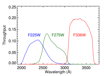
Figure 1.— Throughput of the WFC3-UVIS filters used in the UVUDF: F225W in blue, F275W in green, and F336W in red. These throughputs include the quantum efficiency of the CCD.

We describe the science goals of the project in Section 2; survey strategy and observations in Section 3; we outline data reduction and source extraction in Section 4; we characterize the data quality and discuss issues related to the charge transfer efficiency of the CCD in Section 5. In Section 6 we describe preliminary analysis of the data and initial science results, before summarizing in Section 7. Throughout, we assume a $\Lambda$-dominated flat universe, with $H_{0}=71$ km s^-1 Mpc^-1, $\Omega_{\Lambda}=0.73,$ and $\Omega_{m}=0.27$.

2. Science Goals

2.1. Tracing the evolution of star formation

Observations of UV-bright galaxies trace the evolution of cosmic star formation and provide key constraints on galaxy formation. The UVUDF detects galaxies with star formation rates (SFRs) greater than $\sim 0.05~{}M_{\odot}$/yr at $z\sim 2-3$ (in the absence of dust extinction) with the same UV color selection techniques used at higher redshift. For example, the Lyman break galaxy (LBG) selection, whereby high redshift galaxies are identified by their strong flux decrement at short wavelengths due to the Lyman break feature, is routinely used in many studies (e.g. Steidel et al., 1999; Adelberger et al., 2004; Reddy et al., 2008; Bouwens et al., 2011). When more photometric information is available, more complex methods become available (see Section 2.4). Measuring the combination of the UV luminosity function and the mass function of UV-selected galaxies will provide a statistical picture of the history of star formation in these sources, in redshift slices between $1<z<2.5$ (Lee et al., 2012b). UV-selection in this epoch will enable significant spectroscopic follow-up, with access to vital rest-frame optical diagnostics of extinction, metallicity, and feedback. We provide an initial LBG selection in UVUDF in Section 6.

One of the largest sources of systematic error in estimates of the SFR and the cosmic star formation history is the fact that dust absorbs and reprocesses approximately half of the starlight in the universe (Kennicutt, 1998a). The amount of re-radiated light, quantified by the ratio of integrated IR to UV luminosity, IRX$\equiv$L_IR/L_UV, has been found to be correlated with the UV spectral index, $\beta$ (where $f_{\lambda}\propto\lambda^{\beta}$), in local starburst galaxies (e.g. Meurer et al., 1999). This correlation is routinely used to correct UV SFR estimates for dust attenuation in highly star forming galaxies at all redshifts (e.g. LBGs and BzKs; Adelberger & Steidel, 2000; Daddi et al., 2007; Reddy et al., 2010, 2012a; Kurczynski et al., 2012; Lee et al., 2012a). UV bright galaxies and IR luminous galaxies ($L_{IR}>10^{11}L_{\odot}$) at lower redshifts are found to be broadly consistent with the starburst IRX-$\beta$ correlation (Overzier et al., 2011). Understanding the effects of extinction at high redshift requires detailed study of normal galaxies 7-10 Gyr into the past (the epoch probed by the UVUDF), where both the UV slope and the infrared emission can be measured. (e.g. Boissier et al., 2007; Siana et al., 2009; Swinbank et al., 2009; Buat et al., 2010; Bouwens et al., 2012; Finkelstein et al., 2012).

2.2. The Build-up of Normal Galaxies

The role (and nature) of feedback, and the relative importance of merging in galaxy mass growth are still debated issues. Observations show that “normal” galaxies were in place at $z\sim 1$, with stellar population and scaling relations consistent with passive evolution into the homogeneous population observed in the local Universe (e.g. Scarlata et al., 2007; Cimatti et al., 2008). This situation changes drastically looking back just a few Gyrs. Among the diversity and complexity of massive galaxy types, two types have been extensively studied: gas-rich clumpy disks forming stars at rates of 100 M_⊙/yr that do not have counterparts in the local Universe (e.g. Daddi et al., 2010; Elmegreen et al., 2005; Genzel et al., 2008), and passive objects that are observed to be $\sim$30 times denser than any galaxy today (e.g. Cimatti et al., 2008; van Dokkum et al., 2008). The former are key to understanding the role of instability and gas accretion in the formation of disks and bulges (by migration and merging of the clumps); the latter are important because we do not yet understand the physics of quenching of star formation and the role that compactness plays in it.

It is tempting to think of these well-studied populations as different phases in the formation of local galaxies. Secular evolution of star-forming sub-structures within gas-rich disks could lead to the formation of bulges, and the compactness of high$-z$ spheroids would be the result of the highly dissipative merger of the clumps (Elmegreen et al., 2008; Dekel et al., 2009). Clumps are predicted to be fueled by cold ($T<10^{4}$ K) gas streams that efficiently penetrate the hot medium of the dark matter halo (Kereš et al., 2009). The UV morphology of LBGs at $z=3-4$ are also suggestive of this process (Ravindranath et al., 2006). Furthermore, it is still not clear what mechanism quenches the star formation in the newly formed bulges, what prevents more gas from cooling and forming stars, and what drives the size evolution of compact spheroids.

Current HST observations allow us to derive stellar masses, SFR, surface density of star formation, and the extinction of individual bright clumps at $z\sim 2-3$ by fitting the spectral energy distribution (SED). However, without access to the rest-frame UV, our assessment of star-formation activity becomes poorer at lower redshifts. At $z\sim 2.3$, such structures are found to have sizes of $\sim 1.8$ kpc, typical masses of several $10^{7}M_{\odot}$, and ages of $\sim 0.3$ Gyr (Elmegreen & Elmegreen, 2005).

The UVUDF observations are designed to provide the depth and resolution ($\sim 700$ pc) to study sub-galactic structures at $0.5<z<1.5$ at consistent rest-frame UV wavelengths, offering continuity with measurements at low and high redshift. We confirm the utility of the data for this purpose in Section 6. Measurement of the typical UV sizes and luminosities will constrain stellar-mass and stellar-population properties using the full SED. Finally, the data will enable comparison of the colors of individual sub-galactic units at different radii for the SF galaxies at $z<2$ and $z=3$. A color gradient would be expected if there is migration of previously formed structures towards the center to form the bulge.

2.3. Contribution of galaxies to the ionizing background (below 912 Å)

Star–forming galaxies are likely responsible for reionizing the universe by $z\sim 6$, assuming that a high fraction of Hi–ionizing (Lyman continuum; LyC) photons are able to escape into the IGM. Recent studies suggest that the escape fraction, $f_{esc}$ is higher at high redshift (Shapley et al. 2006; Iwata et al. 2009; Siana et al. 2010; Bridge et al. 2010; Nestor et al. 2013, but see Vanzella et al. 2012). However, it is extremely difficult to directly measure the LyC at $z>4$ due to the increasing opacity of the IGM. Thus, it is important to understand the physical conditions that allow LyC escape at $2<z<3$ and to determine if those conditions are more prevalent during the epoch of reionization.

Ground-based surveys suffer from significant foreground contamination, and from not knowing from which part of the source the ionizing emission is escaping. HST resolved images of both the ionizing and non-ionizing emission of galaxies are necessary to confirm the extreme ionizing emissivities suggested by previous surveys (Iwata et al., 2009; Nestor et al., 2013). The UVUDF filters will enable measurement of the LyC escape fraction at redshifts $z\sim 2.20,2.45,3.1$ in F225W, F275W, F336W, respectively (see Figure 1 for the filter throughputs).

2.4. Improved Photometric Redshifts

Despite intensive spectroscopic surveys that have provided hundreds of redshifts (Szokoly et al., 2004; Le Fèvre et al., 2005; Vanzella et al., 2005, 2006, 2008, 2009; Popesso et al., 2009; Balestra et al., 2010; Kurk et al., 2013), the majority of sources in the UDF are either too faint or otherwise inaccessible. Redshifts must therefore be determined either through color selection or photometric redshifts (photo-z). However, young star-forming galaxies often lack strong continuum breaks in the rest-frame optical, making accurate photo-zs nearly impossible with only optical+NIR data.

The three UVIS filters target the dominant signature of the galaxies’ SEDs in the redshift range $1.2\lesssim z\lesssim 2.7$ – the Lyman break. This feature will allow color selection of these galaxies, and will resolve many of the photo-z degeneracies and thereby improve the photo-z fits. While photo-z’s currently exist for all objects in the UDF (Coe et al., 2006), they often have multiple peaks in their probability distribution functions, $P(z)$, making the true redshift uncertain. In fact, Rafelski et al. (2009) found that the introduction of the ground-based u-band data improved the photo-z’s for 50% of the $z\sim 3$ sample. However, their results suffered from the limited angular resolution and depth of ground-based u-band data (see also Nonino et al., 2009). The F336W filter significantly improves the redshifts from $2\lesssim z\lesssim 3$ and $z\lesssim 0.3$, while the F275W filter improves the redshifts at $1.5\lesssim z\lesssim 2$ and $z\lesssim 0.2$, and the F225W filter improves them at $1\lesssim z\lesssim 1.5$. Figure 2 shows the expected improvement in redshift estimation with the addition of UV data with a sensitivity of AB=29 in each filter. Here we define an unambiguous photometric redshift as one with 95% of the probability distribution function ($P(z)$) to be within $0.1(1+z)$ with only a single distinct peak in $P(z)$.

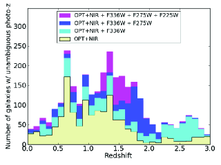
Figure 2.— The expected improvement in the number of unambiguous photometric redshift estimates with the addition of UV filters. Simulated UV fluxes were added to the catalog of Coe et al. (2006) assuming sensitivities of AB=29 in the three UVUDF filters. Photometric redshifts were then calculated and compared to the results without the UV. Estimates determined to have a single, distinct redshift probability peak were taken as unambiguous.

2.5. Star Formation Rate Efficiency of Neutral Atomic-Dominated Hydrogen Gas

The locally established Kennicutt-Schmidt (KS) relation (Kennicutt, 1998b; Schmidt, 1959) relates the gas density and the SFR per unit area, $\Sigma_{SFR}$ $\propto$ $\Sigma_{gas}^{\beta}$. While this assumption is reasonable at low redshift for typical galaxies, it has been shown not to hold for neutral atomic-dominated hydrogen gas at $z\sim 3$ (Wolfe & Chen, 2006; Rafelski et al., 2011). Nonetheless, cosmological simulations often use the KS relation at all redshifts, for both atomic and molecular hydrogen gas (e.g. Kereš et al., 2009).

Damped Ly${\alpha}$ systems (DLAs; see Wolfe et al. 2005 for a review) are large reservoirs of neutral hydrogen gas. At $z\sim 3$, the in situ SFR of DLAs is found to be less than 5$\%$ of what is expected from the KS relation (Wolfe & Chen, 2006). This means that a lower level of star formation occurs in DLAs at $z\sim 3$ than in modern galaxies. Another possibility is that in situ star formation may occur at the KS rate only in DLA gas associated specifically with LBGs. These DLAs are constrained by measuring the spatially extended low-surface-brightness (LSB) emission around LBGs. Rafelski et al. (2011) detect such emission on scales up to $\sim 10$ kpc in a sample of $z\sim 3$ LBG’s (Rafelski et al., 2009) in the UDF F606W image (rest-frame FUV). The emission is measured to $\gtrsim 31$ mag arcsec^-2 and on large scales by stacking $z\sim 3$ LBGs that are isolated, compact, and symmetric. The resulting SFR around LBGs was found to be $\sim 2-10\%$ of what is expected from the local KS relation (Rafelski et al., 2011).

This result can be used to constrain models of galaxy formation at $z\sim 3$. Gnedin & Kravtsov (2010) conclude that the main reason for the decreased efficiency of star formation is that the diffuse ISM in high redshift galaxies contains less dust, and therefore have a lower metallicity and a lower dust-to-gas ratio, which is needed for shielding in order to cool the gas and form stars. This notion matches the observation that DLA metallicities decrease with redshift (Rafelski et al., 2012), and therefore we expect that the efficiency of star formation may be correlated with redshift. This effect must be further understood and taken into account when interpreting models of galaxy formation and evolution.

The transition from the lower star formation efficiencies at $z\sim 3$ to those on the Hubble sequence at $z\sim 0$ may be observable at redshifts in between. We plan to find that transition or constrain when and how it occurs by probing the star formation in the LSB regions around moderate redshift LBGs. It is only in the outer diffuse regions, where the metallicity is lower, that the KS relation is seen to be evolving. The NUV coverage of the UDF enables us to detect this star formation at a range of intervening redshifts by providing significantly improved photo-z’s (Section 2.4) at $z\sim 2-3$ in order to identify LBGs to stack in the optical UDF data, and possibly by stacking the UV data themselves at $z\sim 1$, if the CTE corrected data permit (see Section 5.1.1).

3. Observations

The UVUDF program was executed in three epochs, due to the heavy scheduling constraints on HST in Cycle 19 (Fall of 2011 through Fall of 2012). Table 1 lists the orbit distribution and position angle of each set of observations. In each case, a common pointing center is used: RA: 03 32 38.5471 DEC: -27 46 59.00 (J2000). Figure 3 shows the orientation of each epoch compared to previous UDF programs.

Table 1UVUDF Observing Epochs

Epoch	Observing Window	ORIENT	Orbits per UVIS filter	Orbits per	CCD Readout
			F225W:F275W:F336W	ACS filter	Mode
Epoch 1	March 2$-$March 11 2012	96.0	6:6:6	4:3:11	binning
Epoch 2	May 28$-$June 04 2012	197.25	8:8:10	20:2:2:2	binning
Epoch 3	August 3$-$September 7 2012	264.0	16:16:14	46	post-flash
Total	March - September 2012	$\cdots$	30:30:30	$\cdots$	$\cdots$

Note. — List of orbit distribution and position angle for each set of observations.

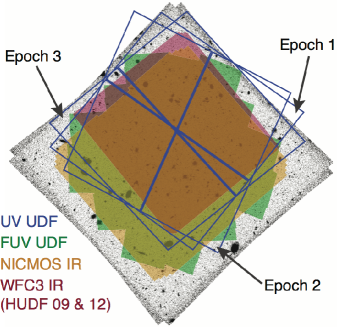
Figure 3.— The footprint of the the UVIS pointing for epochs 1, 2, and 3 are shown as blue squares, with each epoch individually labeled. The greyscale image is the V-band ACS image of the UDF from Beckwith et al. (2006), with North up and East left. The shaded regions are the footprints of other HST imaging of the UDF. The orange represents NICMOS IR (Thompson et al., 2005), the green ACS-SBC FUV (Siana et al., 2007), and the red WFC3 near-infrared imaging from HUDF09 and HUDF12 (Bouwens et al., 2011; Ellis et al., 2013). The readout direction is perpendicular and away from the blue lines marking the chip gap in each epoch, such that the readout is located furthest from the chip gap.

The UVIS focal plane consists of two CCDs, each with $4146\times 2051$ pixels. The plate scale is 0$\farcs$0396/pixel at the central reference pixel. After accounting for the overscan regions, the usable area of each CCD is $4096\times 2051$ pixels. There is a physical gap between the CCDs that corresponds to about 30 pixels (1$\farcs$2).

WFC3/UVIS has a field of view of $162^{\prime\prime}\times 162^{\prime\prime}$, larger than the WFC3/IR channel ($136^{\prime\prime}\times 123^{\prime\prime}$) but smaller than the optical field of the Advanced Camera for Surveys’ Wide Field Camera (ACS/WFC; $202^{\prime\prime}\times 202^{\prime\prime}$; Ford et al., 2002). The UVUDF observations are well matched to the WFC3/IR pointings from two observing programs, as shown in Figure 3. The first program (GO-11563, PI=Illingworth) was excecuted in 2009 (HUDF09; Oesch et al., 2010c, b; Bouwens et al., 2011). The second program (GO-12498, PI=Ellis) was executed after UVUDF at the same pointing as the HUDF09 (Ellis et al., 2013). The footprint of previous UV imaging of the UDF taken with the ACS Solar Blind Channel (SBC) (Siana et al., 2007) and IR imaging taken with NICMOS (Thompson et al., 2005) is also shown in the Figure 3.

Observations were obtained in visits of 2 orbit duration in order to maximize schedulability. Each visit used a single UVIS filter. These visits were linked in groups of 3 in the scheduling instructions to guarantee that all three filters were obtained at the same orientation. During each 2-orbit visit, four exposures were taken. Typically this schedule allowed about 1300 seconds of integration per exposure. In total, we obtained $\sim 82,000$ seconds of integration per filter in the full overlap region (see Table 2). Half the data were taken with binning of the CCD readout, while the other half were taken without binning, but with the use of the post-flash capability (see Section 3.1). The unbinned Epoch 3 exposures were dithered with the standard WFC3-UVIS-DITHER-BOX, which is a 4 point dither pattern with a point spacing of 0$\farcs$173. The binned Epoch 1 and 2 exposures are dithered in an analogous way, but with doubled spacing of 0$\farcs$346.

Table 2UVUDF Sensitivities

Filter	Zero Point	Epoch	Exposure Time	$5\sigma$ 0$\farcs$2 ETC	$5\sigma$ 0$\farcs$2 RMS	50% completeness
	(mag)		(s)	(mag)	(mag)	(mag)
F225W	24.0403	1&2	39278	28.3	28.3	28.6
F275W	24.1305	1&2	39106	28.5	28.4	28.6
F336W	24.6682	1&2	45150	29.0	28.7	28.9
F225W	24.0403	3	44072	27.8	27.9	27.7
F275W	24.1305	3	41978	27.7	27.9	27.7
F336W	24.6682	3	37646	28.3	28.3	28.2

Note. — UVUDF filters, zeropoints, and sensitivities.

An exception to the observing plan occurred in two visits (“1N” and “2H” in the HST schedule), resulting in the loss of both visits in Epoch 2, one for F275W and one for F225W. These visits were rescheduled during Epoch 3 (as visits “5N” and “6H”), and executed as planned at that time.

The area of full overlap between dithered exposures, and thus full sensitivity, is 6.2 arcmin², or 86% of the area of the UVIS detector. The full NUV UVIS overlap region and all of Epoch 3 are completely covered by the deep ACS optical data. The footprint of the UVIS pointing is overlaid on the ACS F606W image of the UDF in Figure 3. The full WFC3/IR pointings (HUDF09 and HUDF12) are covered by the NUV UVIS data.

3.1. Charge Transfer Inefficiency

Over time, radiation causes permanent damage to the CCD lattice, decreasing the charge transfer efficiency (CTE) during readout. The CTE degradation is a serious problem for low background imaging of faint sources, resulting in decreased sensitivity and uncertain calibration for extended sources. The effect is worse for objects that are far from the CCD readout, that is for objects close to the gap between the two detectors in the case of UVIS. The degradation of the UVIS CCDs has been faster than in the early years of ACS, already causing significant signal loss of $\sim 20$% in moderately bright sources (those with $\sim 1000$ e^-/read), and $\sim 50$% for somewhat fainter sources (those with $\sim 300$ e^-/read; Noeske et al., 2012). This faster degradation is believed to be due to the extreme solar activity minimum, and resulting cosmic ray maximum, during the initial flight years of UVIS. The resulting loss of data quality can be partially mitigated by post-processing. The effect is worse for very faint sources, which can be completely lost to “traps” before readout (MacKenty & Smith, 2012; Anderson et al., 2012) and cannot be recovered later. In the literature, CTE degradation is often referred to and measured as charge transfer inefficiency (CTI = 1-CTE) (e.g. Massey, 2010), and we use this terminology interchangeably below.

After Epoch 2 of the UVUDF had already been obtained, the Space Telescope Science Institute (STScI) released a new report on mitigating CTI (MacKenty & Smith, 2012). The strong recommendation is to use the “post-flash” capability of the instrument to illuminate the detector and add background light to the observation. This additional background will fill the traps and ensure that faint objects are not lost, as well as significantly improve the accuracy of pixel-based CTE corrections. This benefit comes at the cost of decreased sensitivity, however, due to the noise introduced by the added background.

Considering that many of the science goals of the UVUDF rely on measuring (or setting limits on) the faintest sources, and require accurate photometry, we chose to follow the recommendation for post-flash. In Epoch 3, we applied a post-flash to bring the average background (the sum of post-flash, sky and dark current) up to about 13 electrons per pixel. In practice, this meant adding 11e^- in F225W and F275W, and 8e^- in F336W. The spatial distribution of post-flash light is not uniform (MacKenty & Smith, 2012; Anderson et al., 2012), so target levels were set to ensure both a reasonable average and a sufficient background in the less illuminated regions.

3.2. Binning the CCD Readout

Without post-flash, the UVIS detectors are read-noise limited in the F225W and F275W filters, even in long exposures such as those needed for the UVUDF. The noise from the readout and from the sky background is about equal in F336W. As a consequence, there is the potential for tremendous sensitivity gain by binning the CCD pixels $2\times 2$ during readout. In principle, $2\times 2$ binning results in a gain of a factor of 2 in signal to noise (S/N) ratio, or 0.75 magnitudes. One concern in the decision to bin the CCD readout is the loss of spatial resolution. However, the large number of repeated observations allow for excellent sub-pixel image reconstruction.

Once the post-flash capability became available to mitigate the effects of CTI, the benefit of binning the CCD readout was greatly reduced. At that point, the signal-to-noise gain would be under 20%, while still reducing the spatial resolution. As a result of these considerations, we chose to take the second half of the UVUDF data, that is Epoch 3, without binning the CCD readout.

3.3. Parallel ACS Observations

Coordinated parallel exposures were obtained with the ACS/WFC3 during the primary WFC3/UVIS observations. Figure 4 shows the location of the parallel fields in comparison to other data in GOODS-South. Table 1 gives the specification for each parallel field, with position angle specified by the HST ORIENT keyword, which is the position angle of the U3 axis, where U3$=-$V3. The V3 angle is an angle based on the reference frame of the telescope, where V3 is perpendicular to the solar-array rotation axis. This angle describes the angle of rotation of the WFC3 UVIS exposure on the sky, and the position and rotation of the parallels.

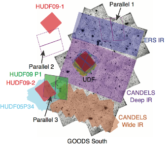
Figure 4.— The footprint of the the ACS parallel pointings for Epochs 1, 2, and 3 are shown as purple squares. The greyscale image is the V-band ACS map of GOODS-South from Giavalisco et al. (2004), with North up and East left. The blue squares and nearby shaded regions indicate the footprint of the UVUDF UVIS pointings and complementary data from Figure 3. The blue shaded region indicates the footprint of the ERS imaging (Windhorst et al., 2011), the purple and brown indicate the footprint for CANDELS Deep and Wide respectively (Grogin et al., 2011), and the shaded red regions indicate the footprint of the near-infrared imaging from the HUDF09 (Bouwens et al., 2011). The green shaded region indicates the footprint of the HUDF09 parallel 1, and the cyan shaded regions represents the HUDF05 parallel P34 (Oesch et al., 2007).

The Epoch 1 parallel exposures fall within the ERS field. The Epoch 2 parallel exposures fall outside of the main CANDELS and GOODS footprint, but still within the field observed by the GEMS program (Rix et al., 2004), and the ground-based U- and R-bands (Nonino et al., 2009). Scheduling constraints did not permit a more favorable orientation. The Epoch 3 orientation was chosen specifically to place the parallel field at the position of the one of the parallels to the HUDF09 (the HUDF09-2 parallel field). The distribution of exposures per filter varies with the position of the parallel data (see Table 1).

The parallels of Epoch 1, which fall within the ERS, consist of 18 orbits. Given the depth of existing data in that field, we chose to obtain images with the three standard optical filters F435W, F606W, F814W. Four orbit depth was obtained in the B-band (F435W), to more than double the previous imaging exposure time. The V (F606W) and wide I-band (F814W) exposure times were chosen so that when combined with previous imaging, the ratio would be $\sim$1:2, following the strategy for parallel imaging in CANDELS (Grogin et al., 2011, their Section 6).

For Epochs 2 and 3, we obtained very deep B-band imaging. There is a growing recognition that HST’s UV and blue optical capabilities are a unique resource which should be used now to prepare for later years when space-based observing will be focused on the near-infrared, with missions such as the James Webb Space Telescope (Gardner et al., 2006), the Wide Field Infrared Survey Telescope (Dressler et al., 2012), and Euclid (Laureijs et al., 2012). With 20 and 46 orbits in Epochs 2 and 3 respectively, we obtained deep-field quality images. At the position of the Epoch 3 parallel field, the HUDF09-2 field has already been observed for 10 orbits in the B-band (Bouwens et al., 2011), enabling a combined deep pointing of 56 orbits of observation. For comparison, the original ACS/WFC3 B-band images of the UDF were also obtained in 56 orbits. We note, however, that the detector performance was better at that time (see Sections 3.1 and 5.1). In Epoch 2, we also obtained shallow imaging in the V (F606W), $i$ (F775W), and $z$ (F850LP) filters, to augment the shallower imaging available from GEMS. The failed visits described in section 3 shifted 4 orbits from planned B-band exposures in Epoch 2 to Epoch 3.

4. Data Reduction

The UVUDF data set consists of four exposures and 2 orbits per visit, with visits divided into three observing epochs as described above. In total, there are 15 visits (30 orbits) for each of the three filters.

In this section, we describe the data reduction process needed to produce science quality images from the UVUDF observations. We plan to release fully reduced images and catalogs at a later time, but not in combination with this paper (see Section 7). Nonetheless, it is important to document the many issues with the data from this HST Treasury program, and for the reader to understand the process that led to the images used for the analysis in the later sections of the paper. The same lessons learned here will be relevant to planning of future UVIS observations.

Binned and unbinned data (and data with and without post-flash) must be processed differently, and they require different calibration files. The software pipeline that we use for UVUDF data begins with the standard Pyraf/STSDAS calwf3 modules, though calibration files needed to be constructed with some care as described in this section. The processing of ACS parallel data closely follows the procedures used by CANDELS (Koekemoer et al., 2011), and is not described here.

4.1. Calibration Pipeline

Calibration exposures (darks, biases, flat fields) for UVIS are obtained by STScI as part of the standard calibration observations. In most cases, these calibrations are taken without binning the CCD readout, though a few binned calibration observations have been obtained. The CCD detectors are periodically heated in order to mitigate hot pixels that develop over time, called annealing. Specifically, $\sim 500$ new hot pixels appear per day, while the annealing process removes $\gtrsim 70$% of hot pixels (Borders & Baggett, 2009). The number of permanent hot pixels that can not be fixed by anneals is growing by 0.05-1% per month (WFC3 instrument handbook). In order to minimize the number of hot pixels at any given time, the detector is annealed once per month.

New calibration files are needed for the calibration pipeline: new biases, darks, and flats for the binned data, and new darks for the unbinned data. Only the bias files used data that were taken with onboard binning. In the other cases, unbinned calibration data are the basis of creating new files, with after-the-fact binning applied where necessary. We validated this latter procedure using the limited set of onboard-binned calibrations that are available. We use a combination of custom scripts and standard STSDAS routines to make these calibration files. The steps involved to construct each type of calibration file are described below.

The standard calibration pipeline begins with an overall bias correction, calculated by fitting the overscan region in a master bias frame, and removing the electronic zero point bias level. Next, a bias reference frame is subtracted from the full image to correct for pixel-to-pixel bias structure. For the binned Epoch 1 and 2 data, this reference file is created using the STScI software wfc3_reference.py (Martel et al., 2008) to average ten onboard-binned bias frame exposures (Baggett, CAL-12798). For the unbinned Epoch 3 data, we use the standard unbinned bias frames provided by STScI.

The next calibration step is the subtraction of a dark reference file to correct dark current structure and to mitigate hot pixels that can cause significant artifacts in the images. STScI releases new darks every 4 days that are based on the average of $\sim 10-20$ dark exposures with integration times of $\sim 900$s each. This is necessary due to the large number of new hot pixels per day, and the drastic change in hot pixels after each anneal. However, binned darks are not obtained on a regular basis. Therefore, unbinned darks are binned after the fact using custom IDL scripts. We validate this approach by measuring the dark current in one set of binned dark exposures obtained for this purpose (Baggett, CAL-12798).

We find the standard processing of the dark calibration is insufficient for the UVUDF data. The STScI-processed darks were created with two choices that are not optimized for this case. First, the process uses an unaggressive definition of a hot pixel as a $\sim 10\sigma$ deviation. The choice results in warm-to-hot pixels not being masked in the UVUDF images, which add significant artifacts to the highly sensitive mosaics. This effect is augmented by CTI causing many hot pixels and their CTI trails to fall below this threshold designed for data without CTI issues. Second, the standard processing uses the median value of the average darks (with hot pixels masked) as the value of all pixels in the dark frame. This median-value dark with hot pixels is the calibration file available from STScI. It is not suitable for UVUDF data, because there is a low-level gradient present in the dark that is not subtracted. This gradient is typically small compared to the sky background in the optical, with a peak-to-valley deviation of $\sim 3$ e^-/pix/hr. However, in the low-background NUV images, it is the dominant structure. While this background can be corrected in the background subtraction phase of the pipeline, it is more accurate to model this background and subtract it before dividing by the flats.

We therefore reprocess the darks, starting with the raw dark observations, using a procedure based on the one provided to us by STScI (J. Biretta, private communication) and the wfc3_reference.py code (Martel et al., 2008). We make two significant modifications to the STScI procedure (Borders & Baggett, 2009) to fix the issues identified above. First, we use an iterative $\sim 3\sigma$ cutoff for defining a hot pixel, applied to cosmic-ray cleaned darks made from the average of a minimum of 10 exposures. This change significantly increases the number of hot pixels masked ($\sim 7\%$ of the image), but decreases the extra systematic noise. Secondly, we fit a $7^{th}$ order polynomial to the remaining non-flagged pixels in the image of each UVIS CCD. Then, we create a final dark frame by combining this polynomial fit, as the background value, and the hot pixels superimposed and flagged in the data quality array. In the case of the binned data, the new darks are binned after the fact.

The next calibration step is the application of the flat field reference files. For the binned data, flats are binned after the fact from the unbinned calibration data. For the unbinned data, the flats provided by STScI are applied. The final calibration step is populating the photometry keywords in the FITS header using the current filter throughput curves and detector sensitivity information using calwf3.

The last processing step is the background subtraction of the individual calibrated images. The unbinned data have an artificial background introduced by the post-flash process. We subtract the post-flash reference files provided by STScI from the unbinned data. These reference files are generated by STScI from stacks of post-flashed exposures, and then scaled to the flash count rate when applied to the data. However, both these post-flash-subtracted images, and the binned images, have a residual nonuniform background. We therefore fit a background to each individual image via a custom inverse distance code. This code masks large fractions of each image for cosmic rays, sources, hot pixels, and bad pixels. It then interpolates the background value at any given pixel based on an inverse-distance weighting within a subgrid region. These backgrounds are then subtracted from all science images. The final products of the calibration pipeline are basic calibrated background-subtracted images, together with data quality maps, that can be used as input to the mosaicking pipeline.

Image registration and mosaicking are performed following the procedures used for CANDELS. We refer the interested reader to Koekemoer et al. (2011). UV mosaics are registered to the ACS B-band image (Beckwith et al., 2006).

4.2. Object Detection and Photometry

We use the Source Extractor software version 2.5 (SExtractor; Bertin & Arnouts, 1996) for object detection and photometry. SExtractor is used in dual image mode, where objects are detected in the deeper F435W (B-band) mosaic (Beckwith et al., 2006), and the photometry is measured in a combined Epoch 1 and 2 mosaic and Epoch 3 mosaic for each filter. In this way, colors of sources are measured using the same isophotal apertures, and fluxes are measured for all B-band detected objects regardless of any flux decrement in the NUV mosaics due to the Lyman Break. Edge regions and the central chip gaps of the mosaics are excluded, and are set to the sky level with the same noise properties as the mosaics such that SExtractor does not find spurious sources along the edges or in the central chip gap.

The detection parameters for the B-band mosaic are tuned such that no sources are detected in the negative image. This is accomplished by setting the minimum area of adjoining pixels to 9 pixels, and a 1$\sigma$ detection threshold. A Gaussian filter is applied on the mosaics, with a full width at half maximum (FWHM) of 3 pixels for object detection. SExtractor is provided an RMS weight map for both the detection and analysis image. The gain parameters are set to the exposure time, such that SExtractor calculates the uncertainties properly. All source photometry has the the local background subtracted by SExtractor, using a local annulus that is 24 pixels wide (with the inner radius depending on source size). Zero points of 24.0403, 24.1305, and 24.6682 are applied for the F225W, F275W, and F336W mosaics respectively (see Table 2). We note that since the B-band is significantly more sensitive than the NUV images, the resulting catalog contains B-band objects too faint to be measured in the UV, and thus cuts on the catalog are used as needed for each scientific purpose.

The photometry of objects is measured with SExtractor using both isophotal and Kron (1980) elliptical apertures. Isophotal apertures are used whenever measuring the color of a source, such as in the color-color selections used in section 6.1. For this purpose, we also run SExtractor on the F606W (V-band) mosaic (Beckwith et al., 2006) in dual image mode, still using the B-band as the detection image. This procedure results in aperture-matched photometry, although it is not corrected for variation in the point-spread function (PSF). Since the PSFs of the NUV and the optical B- and V-bands are quite similar, this correction will be small for these bands. For this overview paper, these color measurements are sufficient. Uncertainties will be dominated by CTI effects (see section 5.1). Kron elliptical apertures are used to measure the total magnitude of each source via SExtractor’s MAG_AUTO parameter. These magnitudes measure the total flux from a source, and are used whenever a total magnitude is needed, such as in the number counts of LBGs (see section 6.1).

5. Data Characterization

5.1. CTI effects

Radiation damage sustained by the CCD degrades its ability to transfer electrons from one pixel to the next, trapping electrons (in part temporarily) during readout, while other electrons are moved to the next pixel. This results in trails of electrons in the direction of the CCD readout, with regions of the CCD furthest from the readout affected most severely (e.g., Rhodes et al., 2010; Massey et al., 2010, and the references therein). The three different orientations of the three UVUDF epochs enables the measurement of CTI effects in the data. Specifically, Epoch 1 and 2 are at an angle of 101.25 degrees relative to each other, resulting in some galaxies located close to the readout in one epoch, and far from the readout in the other (see Figure 3). This configuration allows the characterization of the effect of CTI on the photometry and morphology, as well as an estimate of the number of faint galaxies that are completely lost.

5.1.1 Corrections for CTI

There are currently two methodologies to correct the photometry for CTI losses. The best method is a pixel-based CTE correction of the raw data based on empirical modeling of hot pixels in dark exposures (Anderson & Bedin, 2010; Massey et al., 2010). Such a correction not only corrects the photometry, but also restores the morphology of sources (see section 5.1.3). A preliminary version of software to implement such a correction for unbinned WFC3/UVIS data was released in March 2013, but significant improvements and verification will be needed before the correction is stable enough to warrant the public release of corrected high level science products for the UVUDF. There are three major issues that need to be overcome for the software to fully support the UVUDF data: 1) The code only works for unbinned data, and half the UVUDF data are binned. 2) The current algorithm over predicts the CTE correction for low background faint sources (Anderson, 2013), and the binned half of the data have very low backgrounds. 3) Read noise mitigation in the algorithm results in under-correction for faint sources (Anderson, 2013). The WFC3 team at STScI is aware of the latter two limitations and is working on improvements. In addition, while the post-flash Epoch 3 data can have the CTE algorithm applied in a straightforward manner, post-flashed CTE corrected darks are required to match the hot pixels.

The second method to mitigate the effect of CTI is to apply a correction to the measured flux densities of sources, based on their location on the detector, the observation date, and their flux in electrons (e.g. Cawley et al., 2001; Riess & Mack, 2004; Rhodes et al., 2007; Noeske et al., 2012, Bendregal et al. 2013). However, the current WFC3 UVIS implementation of this catalog-based calibration (Noeske et al., 2012) has many limitations. First, it can only be applied for a small number of quantized background levels, including virtually no background, $\sim 3$e^-/pix, and 20-30e^-/pix. Thus, it is only applicable to the UVUDF Epoch 1 and 2 data for F275W and F225W, and these corrections have slightly higher backgrounds than the UVUDF data. The F336W data and all the Epoch 3 data have backgrounds that are not similar to any of the standard calibrations. The poor sampling of background levels in the calibrations makes interpolating between them unreliable. Second, the calibration was measured for relatively bright point sources, and the correction is uncertain at the faint end, which encompasses the majority of UVUDF sources. Third, it does not take into account other nearby sources which can fill charge traps and thereby shield the sources. Lastly, it does not take into account the morphology of sources (i.e. size and shape), and therefore does not account for effects such as self-shielding that accompany non-point sources, as electrons from the part of the source closer to the readout will shield the other part from charge traps.

Keeping these several limitations in mind, we apply the Noeske et al. (2012) correction to the F225W and F275W mosaics of Epochs 1 and 2 separately. This correction enables us to refine our investigation of the effects of CTI (e.g. Sections 5.1.2 and 5.1.4). However, we can not apply the calibration to the combined Epoch 1 and 2 mosaic nor the F336W mosaics, so the science investigations in Section 6.1 do not include the correction. Those investigations use the combined Epoch 1 and 2 mosaic, which partially mitigates the CTI effect because objects far from the readout in one epoch are averaged with their counterparts closer to the readout in the other epoch. Future work using this data will apply the pixel-based CTE correction (when it is stable) to obtain more reliable photometry.

5.1.2 CTI effects on photometry

In order to characterize the CTI in the UVUDF data, a new catalog was created, with a method differing from that described in section 4.2. For each single epoch mosaic in each filter, SExtractor was run in dual image mode, with the combined Epoch 1 and 2 mosaic as the detection image. The detection threshold was set such that we do not detect sources in the negative image. Objects near the edges or near the chip gaps for any of the three epochs were excluded, and objects were required to be covered by all three epochs of observation. The catalog was trimmed to only include sources with S/N ratios greater than 5$\sigma$ in all three single epoch mosaics. Galaxies in the NUV images are often clumpy, which results in single galaxies appearing as multiple clumps in the images. Regardless of the deblending parameters used with SExtractor, these galaxies are detected as separate sources. This is not an issue for the CTI measurements described below, and the main catalog is not strongly affected by this, since the B-band is used as the detection image in that case.

The effects of CTI are worst in exposures with low background (MacKenty & Smith, 2012), thus the measured UVUDF CTI effects are described for F275W, which has a lower background than F336W, yet sources are brighter than in F225W, enabling us to measure more sources. Specifically, the unbinned equivalent average backgrounds are $\sim 5.8$ e^-/pix/hr, $\sim 6.2$ e^-/pix/hr, and $\sim 12.2$ e^-/pix/hr for F225W, F275W, and F336W exposures, corresponding to $\sim 2.4$ e^-/pix, $\sim 2.5$ e^-/pix, and $\sim 5.1$ e^-/pix in the half orbit exposures used. The backgrounds in F225W and F275W are consistent with the expected value due to dark current. The CTI effects are present in all three bands, but expected to be at a lower level in the higher-background F336W mosaics. The basic effect of CTI on the photometry is that the objects lose a fraction of their flux proportional to their distance from the readout, as electrons encounter more charge traps the further they travel.

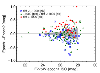
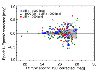
Figure 5.— Photometry comparison of sources in Epochs 1 and 2 F275W mosaics illustrating a larger photometric scatter than expected from the uncertainties, likely due to CTI effects. For objects far from the readout, the actual 1$\sigma$ dispersion is larger by more than a factor of 2 than expected. Both panels are the same except that the bottom panel includes a catalog based CTE correction for both Epochs 1 and 2 assuming point source morphology (see Section 5.1.1). The difference in isophotal magnitudes between Epochs 1 and 2 should be zero, with a scatter that increases with increasing magnitude. The black line is the zero difference line, and the expected 1$\sigma$ dispersion is shown as the gray shaded region from uncertainties as measured by Source Extractor. The colors denote the difference in source distance to readout between the epochs. The blue open squares are sources close to the readout in Epoch 1 and far from the readout in Epoch 2, the green filled triangles are sources an intermediate distance from the readouts, and the red filled circles are sources far from the readout in Epoch 1 and close to the readout in Epoch 2.

The uncorrected photometry of Epochs 1 and 2 are compared in the top panel of Figure 5, which plots the difference in isophotal magnitude of Epoch 1 and 2 as a function of the Epoch 1 isophotal magnitude. The scatter is much larger than the expected 1$\sigma$ dispersion (shown as the gray shaded region) likely due to the effects of CTI. For objects far from the readout, the actual 1$\sigma$ dispersion is larger by more than a factor of 2 than expected. The photometric scatter is characterized as a function of the difference in distance to the readout between the epochs, as measured on the drizzled images. When the difference is a large negative number, the sources are close to the readout in Epoch 1 and far from the readout in Epoch 2 (open blue squares). When the difference is a large positive number, the sources are close to the readout in Epoch 2 and far from the readout in Epoch 1 (red filled circles). If CTI is the cause of the large scatter, then the expected behavior is for the blue squares to be primarily below the zero line, and the red circles to be primarily above the zero line. This behavior is indeed what is observed, confirming that CTI is the most likely cause of the large observed scatter.

The CTE-corrected photometry of Epochs 1 and 2 are compared in the bottom panel of Figure 5, which plots the same quantities as the top panel, with the addition of a catalog-based CTE correction (see Section 5.1.1). The CTE correction reduces the scatter observed in the top panel, and it removes the systematic offset of the red circles furthest from the readout. However, the scatter remains larger than expected, possibly due in part to the limitations of the catalog-based CTE corrections described in Section 5.1.1. On the other hand, the scatter could result from imperfect image registration, or CTI effects on source morphology causing inappropriate apertures to be used in the photometric measurements (see Section 5.1.3). The image registration is unlikely to be the cause, because the Epoch 1 and 2 have relative astrometric accuracy of better than 0$\farcs$05. It is possible that the CTI effects on source morphology is the cause, though the use of the combined Epoch 1 and 2 mosaic as the detection image somewhat reduces this effect (but see Section 5.1.3).

We test the hypothesis that something other than CTI is the cause of the scatter by making a comparison that is mostly insensitive to the distance to the readout. We compared two subsets of the Epoch 2 data, each consisting of half the exposures (2a and 2b). Figure 6 plots the difference in isophotal magnitude between the two halves of the Epoch 2 data as a function of the Epoch 2a isophotal magnitude. The points are color coded by distance to the readout, as no difference in readout distance exists. Regardless of the distance to the readout, magnitude differences are consistent with random scatter, although with a slightly larger magnitude than expected from the measurement uncertainties (gray shaded 1$\sigma$ dispersion). This minor remaining difference is most likely due to a slight underestimation of the uncertainties by SExtractor, possibly caused by SExtractor not including the uncertainty in local sky subtraction. It has been noted several times in the literature that SExtractor underestimates the true uncertainties (Feldmeier et al., 2002; Labbé et al., 2003; Gawiser et al., 2006; Becker et al., 2007; Coe et al., 2013).

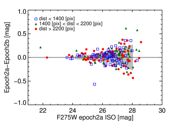
Figure 6.— Photometry comparison of Epochs 2a and 2b F275W with a photometric scatter mostly consistent with that expected from the uncertainties. No correction for CTI is applied, because the correction would be a function of distance to the readout and therefore the same in both halves of the epoch 2 data. The expected 1$\sigma$ dispersion is shown as the gray shaded region. The blue open squares are sources close to the readout ($<700$ pixels away), the green filled triangles are sources an intermediate distance from the readout ($>700$ pixels and $<2200$ pixels away), and the red filled circles are sources far from the readout ($>2200$ pixels away). Regardless of distance to the readout, source magnitudes are mostly consistent with the 1$\sigma$ scatter (gray shaded region).

Another method to visualize the CTI effects is to plot the magnitude difference in Epochs 1 and 2 versus the difference in distance to the readout (top panel, Figure 7). Sources falling to the left in this figure are close to the readout in Epoch 1 and far from the readout in Epoch 2, while sources falling to the right in this figure are close to the readout in Epoch 2 and far from the readout in Epoch 1. Sources for which electrons travel larger distances to the readout lose more flux, so CTI effects would cause the difference in magnitude to be negative in the left half of the figure and positive in the right side of the figure. The sources used in the figure are color coded by magnitude, with purple triangles representing the brightest, and green circles representing the faintest. The purple triangles have a smaller scatter, consistent with the fact that bright sources are less severely affected by CTI than faint sources (Massey, 2010). The red points with error bars in Figure 7, which show the average values in bins of equal numbers per bin, emphasize the trend. The uncertainties are the standard deviation of the points in each bin divided by the square root of the number of points per bin. The bottom panel of Figure 7 is the same as the top, with the addition of a catalog-based CTE correction (see Section 5.1.1). The CTE correction somewhat reduces the scatter observed in the top panel, and removes the slope observed in the data.

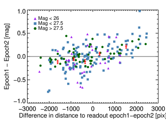
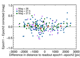
Figure 7.— Photometry comparison of sources in Epochs 1 and 2 F275W mosaics as a function of the difference in distance to readout. Sources falling to the left in this figure are close to the readout in Epoch 1, and far from the readout in Epoch 2, while sources falling to the right in this figure are close to the readout in Epoch 2, and far from the readout in Epoch 1. Sources are color coded by their Epoch 1 magnitudes. The black line is the zero difference line. The red points with error bars are average binned values, with equal numbers of sources in each bin. Observed photometry is consistent with CTI effects, with the difference in magnitudes being negative in the top side of the figure, and positive in the right side of the figure. The slope of the effect is removed (bottom panel) when applying the catalog based CTE correction (see Section 5.1.1).

Given that the increased photometric scatter is correlated with the readout direction, and that there is significantly less scatter when comparing the subsets of Epoch 2 data, we conclude that CTI is the dominant cause of the large scatter in photometry observed in Figures 5 and 6. It is possible that other calibration issues contribute as well, but they would require effects that are also dependent on source position on the detector.

5.1.3 CTI effects on morphology

CTI affects the shape of galaxy images as well as their photometry. Rhodes et al. (2010) investigated the effects of CTI on galaxy morphology using simulations and found that small galaxies are more affected by CTI than large ones. They also found that small bright galaxies are slightly less affected by CTI than small faint ones, but this dependence is not observed for large galaxies. The net effect of CTI on image morphology is a smearing out of the flux in the readout direction. Thus CTI results in circular objects appearing elongated in the readout direction.

This elongation effect is observed in the UVUDF data, as shown in the example in Figure 8. This galaxy is located about two thirds the length of the detector away from the readout in Epoch 1, and almost as far as possible from the readout in Epoch 2. In this example, both the bright galaxy and the nearby smaller structures are elongated in the readout direction, as marked by the red lines. The near 90 degree separation of Epochs 1 and 2 shows the magnitude of the elongation in each direction. We note that this elongation also affects the astrometry, limiting the precision of the alignment between epochs and between UVIS and ACS images.

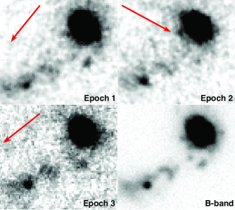
Figure 8.— Example of a galaxy affected by CTI in the F275W images. The top left panel is from Epoch 1, the top right panel is from Epoch 2, the bottom left panel is from Epoch 3, and the bottom right panel is the B-band image. The red arrows correspond to the readout direction, and the galaxy is elongated in the readout direction in each case. The elongation is worst in Epoch 2, as it is furthest from the readout in that Epoch. The elongation is reduced in the post-flashed Epoch 3 compared to Epoch 1.

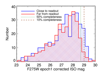
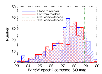
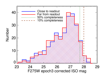
Figure 9.— Histograms of sources detected in the F275W Epoch 1, 2, and 3 mosaics based on their isophotal CTE corrected magnitudes. Sources are split into two groups based on distance to the readout, with sources in the halves of the chips close to the readout shown in blue, and the sources in the other halves far from the readout shown in red. The 50% and 10% completeness levels (see section 5.2) are plotted in green and brown respectively. Sources close to the readout appear to have a tail beyond the 10% completeness, while sources far from the readout drop more steeply. This suggests that we are losing sources far from the readout that are not lost close to the readout.

5.1.4 CTI effects resulting in source loss

Another effect of CTI on the images is the possibility of losing faint sources completely. Studies of warm pixels in long dark exposures show that the number of warm pixels decrease drastically further away from the readout, and the effect is worse for fainter warm pixels (MacKenty & Smith, 2012). That study is a worst case scenario, because warm pixels are not shielded by other nearby pixels as is the case for pixels associated with faint astronomical sources. Nonetheless, post-flash calibration observations of Omega Centuri confirm that faint sources in low backgrounds can disappear completely due to CTI (Anderson et al., 2012). The sensitivity limit of observations is thus set by the exposure time of each individual exposure rather than the average of a stack. This depth varies as a function of distance to the readout, morphology, and position of other sources on the detector.

A simple test of source losses is a comparison of the number counts of detected objects as a function of magnitude for sources close and far from the readout. We start with the B-band selected catalog described in Section 4.2, and consider sources down to $10\sigma$ detections in the B-band and 3$\sigma$ detections in F275W. Except for Epoch 3, we apply the catalog based CTE correction (see Sections 5.1.1 and 5.1.2) to reduce the effects of CTI on the photometry. The prediction is that some sources far from the readout in Epochs 1 and 2 will be lost completely, while source losses should be greatly reduced in the post-flashed Epoch 3 data.

A histogram of detected sources based on their isophotal CTE-corrected magnitudes is shown in Figure 9 for all three epochs. For Epochs 1 and 2, more faint sources are found close to the readout (blue) than are found far from the readout (red), suggesting that some sources far from the readout have been lost. There is no significant difference in the number of B-band sources in the same sample areas.

The sources lost due to CTI are very faint, and the number counts at these faint magnitudes are suppressed by the incompleteness due to lack of sensitivity (Section 5.2). It is therefore difficult to distinguish sources lost due to CTI from sources that would not be detected because of insufficient sensitivity. Most of the losses from CTI are at magnitudes close to the 10% completeness limit for the Epoch 1 and 2 F275W mosaics. Keeping this limitation in mind, as well as the small number statistics at the faintest magnitudes where incompleteness is very high, we estimate the number of lost sources by comparing the number counts close to and far from the readout. For sources fainter than the 50% completeness limit of AB$\sim$28.3 mag (see section 5.2), we find that at least $\sim 30$ sources are lost in each Epoch 1 and Epoch 2 (out of $\sim$600 source positions that are common between the epochs), while no sources are lost in Epoch 3 (out of $\sim 500$). The total number of lost galaxies is likely larger than those found above, because sources in the middle of the CCDs may also be lost. These sources are not close to the readout in either Epochs 1 and 2 and fall below the sensitivity limit of Epoch 3, making them difficult to identify. We expect that the number of these sources per area is smaller than the number found far from the readout, suggesting the total number of lost sources is likely within a factor of two of those observed to be lost. Our best estimate is a loss of $\lesssim 100$ sources out of $\sim$600. The small number of losses suggests that the results presented in Section 6.1 are not strongly biased due to CTI.

Another empirical test of source losses due to CTI is to compare individual sources that are detected close to the readout in one epoch but whose position is far from the readout in another epoch. The Epoch 2 mosaic is slightly more sensitive than the Epoch 1 mosaic (8 orbits F275W in Epoch 2 compared to 6 orbits for Epoch 1), so sources that are detected in Epoch 1 close to the readout, but not detected in Epoch 2 far from the readout demonstrate the effect. In searching for such sources, we also required them to be detected in the significantly more sensitive B-band image (Beckwith et al., 2006). There exist a few such sources, and an example is shown in Figure 10. The left panel is a cutout of the F275W Epoch 1 mosaic and the middle panel is from Epoch 2, and the right panel is from Epoch 3. This source is observed in the optical ACS images, and is object 4188 in the catalog by Coe et al. (2006). It has an F275W isophotal magnitude of $28.6\pm 0.1$, and a F435W total magnitude of $27.9\pm 0.06$ (Coe et al., 2006). This source is detected at $8\sigma$ in Epoch 1, and should have been observed at least at that S/N in the Epoch 2 data.

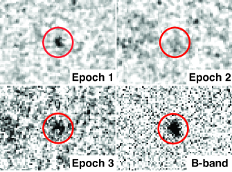
Figure 10.— Example of a galaxy lost due to CTI in the F275W Epoch 2 mosaic. The left panel is a cutout of the F275W Epoch 1 mosaic, the middle panel is from the Epoch 2 mosaic, and the right panel is from the Epoch 3 mosaic. The galaxy is present in the shallower Epoch 1 data which is close to the readout, and is not detected in the slightly more sensitive Epoch 2 data which is far from the readout. This galaxy is observed in the optical ACS images, and is object 4188 in the catalog by Coe et al. (2006). It has an F275W isophotal magnitude of $28.6\pm 0.1$, and a F435W total magnitude of $27.9\pm 0.04$ (Coe et al., 2006). The galaxy is detected at $8\sigma$ in Epoch 1, and should have been observed at a higher significance in Epoch 2 were it not for CTI. The galaxy is also detected in the shallower post-flashed Epoch 3.

The potential loss of faint objects is one of the primary reasons that we decided to use the post-flash option in Epoch 3. The other motivations for the post-flash include reducing other CTI effects and significantly improving pixel-based CTE corrections by taking data with higher backgrounds (MacKenty & Smith, 2012).

The evidence that no sources have been lost in Epoch 3 is encouraging, though the sensitivity limit is necessarily worse. While the F275W exposure time in Epoch 3 is about double that of Epochs 1 and 2 individually, Epoch 3 is significantly less sensitive (see Section 5.2). In fact, most of the sources that appear to be lost in Epochs 1 and 2 due to CTI would not have been detected in the Epoch 3 mosaic in the first place. Thus there are very few examples of sources that were lost in either of the Epochs without post-flash but are present in Epoch 3. One such example is shown in Figure 11. This galaxy is observed in the optical ACS images, and is object 8020 in the catalog by Coe et al. (2006). It has an F275W isophotal magnitude of $27.8\pm 0.1$, and a F435W total magnitude of $27.9\pm 0.04$ (Coe et al., 2006). The source is detected at $9\sigma$ in Epoch 3, and would have been easily detected in both Epochs 1 and 2 were it not for CTI.

It is difficult to measure precisely how many sources may have been lost in Epoch 1 and 2 due to the effects of CTI. We can estimate the magnitude of the problem by referring to the comparison presented in Figure 9. Significantly more faint sources are detected at positions on the CCD close to the readout than far away from it in Epochs 1 and 2, which lack the additional post-flash background. If objects were evenly distributed on the detector, which they may not be, the histograms would suggest that $\sim 5$% of the total sources may have been lost to the effects of CTI, and as many as $\sim 30$% of sources fainter than the 50% completeness limit.

The CTI effects create a dichotomy between the first two UVUDF epochs and the third epoch. The combined Epoch 1 and 2 mosaic is more sensitive than the Epoch 3 data, but suffers more from CTI, and some objects may be lost completely. Once pixel-based CTE corrections are applied, the Epoch 3 data will be the best characterized NUV mosaic available. We agree with the STScI recommendation that future WFC3 UVIS observations that require very sensitive measurements use the post-flash.

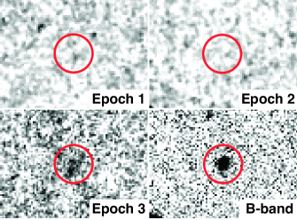
Figure 11.— Example of a galaxy lost due to CTI in the F275W Epoch 1 and 2 mosaics, but preserved in Epoch 3 due to post-flash. The left panel is a cutout of the F275W Epoch 1 mosaic, the middle panel is from the Epoch 2 mosaic, and the right panel is from the Epoch 3 mosaic. The galaxy is present in the shallower Epoch 3 data, and is not detected in the more sensitive Epoch 1 and 2 data. The galaxy is approximately in the middle of the chip in all three epochs. This galaxy is observed in the optical ACS images, and is object 8020 in the catalog by Coe et al. (2006). It has an F275W isophotal magnitude of $27.8\pm 0.1$, and a F435W total magnitude of $27.9\pm 0.04$ (Coe et al., 2006). The galaxy is detected at $9\sigma$ in Epoch 3, and would have been easily detected in both Epochs 1 and 2 were it not for CTI.

5.2. Sensitivity

We use two common methods to characterize the sensitivity of the UVUDF data. First, we measure the sky fluctuations of the images. Secondly, we measure the 50% completeness limit, measured by recovery of simulated sources placed in the science mosaics. The completeness test takes into account both the sky surface brightness and the spatial resolution of the mosaics, yielding a good sense of the usable depth of an image (Chen et al., 2002; Sawicki & Thompson, 2005; Rafelski et al., 2009; Windhorst et al., 2011).

The sky noise of each image is measured via the pixel-to-pixel rms fluctuations. These fluctuations are measured in 51$\times 51$ pixel boxes at 1000 semi-random locations, such that the boxes are entirely on the image, do not fall on a detected object, and the boxes do not overlap other boxes. This technique is designed to be less sensitive to any residual gradient in the image than simply using the rms of all unmasked pixels. The rms in each mosaic is the iterative sigma clipped mean of the rms in each box, which is determined with an iterative sigma clipped standard deviation. This rms is then multiplied by the noise correlation ratio to account for the correlated noise from drizzling the mosaics. The approximate correlation ratio of the UVUDF data is $\sim 2.5$ and $\sim 1.5$ for the binned and unbinned data, respectively, based on equation 9 from Fruchter & Hook (2002). These rms values corrected for correlated noise match the expected values from the rms images. The resulting $5\sigma$ rms magnitudes (assuming 0$\farcs$2 radius aperture) for the mosaics are tabulated in Table 2. These values are within $0.1-0.2$ mags of the 0$\farcs$2 aperture, $5\sigma$ magnitudes predicted by the STScI exposure time calculator modified for binning or post-flash (see Table 2).

We performed a standard completeness test to confirm the noise characteristics of the data by planting and recovering simulated objects. This test does not take into account the loss of sources at the faint end due to CTI, and so the results of the test are an upper limit on the completeness. Specifically, the 50% completeness magnitude limit due to noise is measured by planting Gaussian PSFs for a range of magnitudes in the mosaics at semi-random locations, and counting the fraction of sources that are recovered with SExtractor. The PSF FWHMs are matched to those measured in the data for each filter. Unresolved sources are selected from the published catalogs of stars in the UDF (Pirzkal et al., 2005). However, there are only a small number of identified sources bright enough in the NUV to be used for PSF determination. Three sources are used for F336W, and two sources are used for F225W and F275W. The sources are each registered to their subpixel centers, normalized by the peak value, and coadded with a mean. The resulting PSFs are worse than measured by Windhorst et al. (2011) in the ERS, because half the data are binned and CTI affects the source morphology. For the combined Epoch 1 and 2 mosaic, we measure PSF FWHMs of 0$\farcs$133,0$\farcs$133, and 0$\farcs$127 for F225W, F275W, and F336W. For the Epoch 3 mosaic, we measure PSF FWHM’s of 0$\farcs$134, and 0$\farcs$121 for F275W and F336W, and use the F275W PSF for the F225W PSF as it is not well determined. The locations of the planted sources are constrained such that they do not fall off the edges, fall on a real detected object, or fall on any previously planted source. The detection efficiency as a function of magnitude is shown in Figure 12, and the 50% completeness magnitudes are tabulated in Table 2.

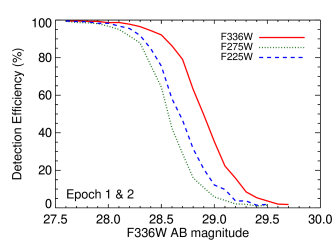
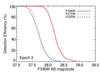
Figure 12.— Detection efficiency of the Epochs 1 & 2 (top) and Epoch 3 (bottom) mosaics as a function of total magnitude. These are the recovery percentages of simulated point sources in the images. The limiting magnitude is defined as the magnitude at which 50% of the sources are recovered. The limiting magnitudes for Epoch 1&2 are 28.6, 28.6, and 28.9 mag, and for Epoch 3 are 27.7, 27.7, and 28.2 mag, for F225W, F275W, and F336W (see Table 2). This completeness test does not account for source losses due to CTI.

6. Initial Results

In this section, we briefly present initial results, representative of those that will be possible with the UVUDF. We describe the color selection of galaxies using the Lyman break technique, and we demonstrate the utility of the deep NUV images for morphological analysis. In both cases, these results are presented based on the combined Epoch 1 and 2 mosaics, without the application of the pixel-based CTE correction. We anticipate that future papers will improve the analysis once that correction is stable and can be confidently applied.

6.1. Lyman Break Galaxies

The selection of high redshift galaxies by the identification of the strong Lyman break feature in their SED using broad-band photometry has been extremely successful (e.g. Steidel et al., 1996b, a, 1999, 2003; Adelberger et al., 2004; Bouwens et al., 2004, 2006, 2010, 2011; Rafelski et al., 2009; Reddy et al., 2008; Reddy & Steidel, 2009; Reddy et al., 2012b). Although less precise than a full SED-fit such as those used in photometric redshift estimates, the Lyman break identification is a standard in the literature. Here, we have taken a first look at selecting LBGs in the UVUDF at redshifts where the Lyman break falls in the NUV filters: 1.7, 2.1, and 2.7 in F225W, F275W, and F336W, respectively. We directly compare these initial results with published results from the ERS (Windhorst et al., 2011), which used the same filters in shallower data (AB=26.9) over a larger area (about 50 square arcminutes).

We implement the dropout criteria used on ERS data by Hathi et al. (2010) (hereafter H10) and Oesch et al. (2010a) (hereafter O10). These consist of both color-color criteria as well as S/N criteria for candidates to be considered dropouts.

Faint stars were removed from the sample by position matching sources in the UVUDF catalog with the published catalog of unresolved sources in the UDF (Pirzkal et al., 2005). 25 sources are found to match this catalog (0.1^′′ matching radius); 22 of these sources are identified as stars according to the criteria of Pirzkal et al. (2005). There are 7, 10, 18 stars detected at S/N = 3 threshold in F225W, F275W, F336W, respectively.

Table 3Summary of Dropout Galaxies in ERS and UVUDF.

Dropout		ERS				UVUDF (ERS Depth)				UVUDF (Full Depth)
		Predicted	Observed			Predicted	Observed			Predicted	Observed
				Surface				Surface				Surface
Filter	Method	Number	Number	Density		Number	Number	Density		Number	Number	Density
(1)	(2)	(3)	(4)	(5)		(6)	(7)	(8)		(9)	(10)	(11)
F336W	H10	394	256	5.1		49	$37\pm 6.6$	$6.0\pm 1.1$		185	$211\pm 14.5$	$34\pm 2.3$
$z\sim 2.7$	O10	448	403	8.6		56	$67\pm 8.2$	$10\pm 1.2$		224	$304\pm 17.4$	$49\pm 2.8$
F275W	H10	228	151	3.0		28	$22\pm 5.2$	$3.5\pm 0.8$		86	$88\pm 9.4$	$14\pm 1.5$
$z\sim 2.1$	O10	102	99	2.1		13	$10\pm 3.7$	$1.6\pm 0.6$		125	$146\pm 12.1$	$24\pm 2.0$
F225W	H10	62	66	1.3		8	$4\pm 2.5$	$0.6\pm 0.4$		36	$25\pm 5.5$	$4.0\pm 0.9$
$z\sim 1.7$	O10	99	60	1.3		12	$9\pm 3.5$	$1.5\pm 0.6$		111	$61\pm 7.8$	$9.8\pm 1.3$

Note. — Column (1) indicates the dropout filter and redshift bin. Column (2) indicates the reference to the dropout method and luminosity function used to identify and predict source counts: H10 (Hathi et al., 2010); O10 (Oesch et al., 2010a). Columns (3-11) compare predicted and observed source counts for each dropout type. ERS refers to the Early Release Science data (Windhorst et al., 2011). UVUDF(ERS) refers to UVUDF data analyzed to a comparable depth as ERS, UVUDF(Full) refers to UVUDF data analyzed to its full depth. Dropout sky density values are in units of arcmin^-2. Uncertainties on the observed number and density of sources are Poissonian. Errors to predicted source counts are discussed in the text.

6.1.1 F336W, F275W, F225W Dropouts

For reference, the H10 criteria for dropout galaxies are given below. F336W dropouts require observed magnitudes and signal-to-noise ratios, S/N, satisfy each of the following

$$\begin{cases}F336W-F435W>0.8\\ F435W\leq 26.5\\ F435W-F606W<1.2\\ F435W-F606W>-0.2\\ F336W-F435W>0.35+[1.3\times(F435W-F606W)]\\ S/N(F435W)>3\\ S/N(F336W)<3\\ S/N(F275W)<1\\ S/N(F225W)<1\end{cases}$$ (1)

Similarly, F275W dropouts are identified by the criteria:

$$\begin{cases}F275W-F336W>1.0\\ F336W\leq 26.5\\ F336W-F435W<1.2\\ F336W-F435W>-0.2\\ F275W-F336W>0.35+[1.3\times(F336W-F435W)]\\ S/N(F336W)>3\\ S/N(F275W)<3\\ S/N(F225W)<1\\ \end{cases}$$ (2)

F225W dropouts require all of the following criteria:

$$\begin{cases}F225W-F275W>1.3\\ F275W\leq 26.5\\ F275W-F336W<1.2\\ F275W-F336W>-0.2\\ F225W-F275W>0.35+[1.3\times(F275W-F336W)]\\ F336W-F435W>-0.5\\ S/N(F275W)>3\\ S/N(F225W)<3\\ \end{cases}$$ (3)

Figures 13, 14, and 15 illustrate the dropout candidates selected according to the H10 criteria in color-color diagrams. Sources with S/N $<1$ in the dropout band have their fluxes replaced with $1\sigma$ upper limits and are indicated as arrows in the figures. Stars are indicated as blue asterisks. Dropout candidates (defined as meeting all of the criteria of H10) are indicated as red symbols. The mean and 1$\sigma$ redshift distributions reported in Hathi et al. 2010 were: (F225W; 1.51, 0.13: F275W; 2.09, 0.42: F336W; 2.28, 0.4). Likewise, the mean and 1$\sigma$ redshift distributions reported in Oesch et al. 2010 were: (F225W; 1.5, 0.2: F275W; 1.9, 0.2: F336W; 2.5, 0.2)

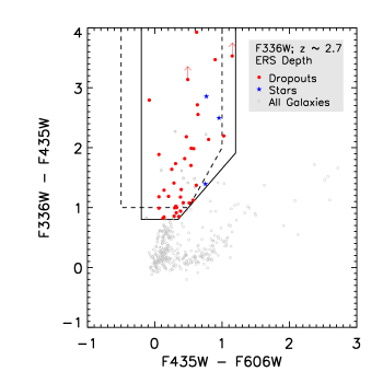
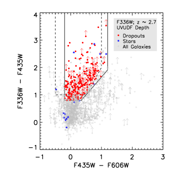
Figure 13.— (left panel) Color-color diagram illustrating F336W dropout candidates in UVUDF to ERS depth using the method of Hathi et al 2010 (H10). Colors are computed from subtracting magnitudes in the appropriate HST wavebands. Sources are illustrated to ERS depth (F435W = 26.5 AB) and have S/N degraded to match ERS observations (as discussed in the text). Red circles are dropout galaxies according to criteria of H10. Stars are indicated as blue asterisks, and upper arrows indicate non-detections in the dropout band replaced with a 1$\sigma$ upper limit. Gray points indicate all sources in the UVUDF catalog to this depth limit; gray points in the color selection region fail to meet the S/N criteria of bona fide dropout galaxies. Solid lines indicate the color-selection region of H10; dashed lines indicate the color-selection region of O10. (right panel) Color-color diagram illustrating F336W dropout candidates to the full depth of UVUDF. Colors and symbols are the same as in the left panel.

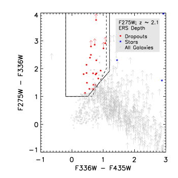
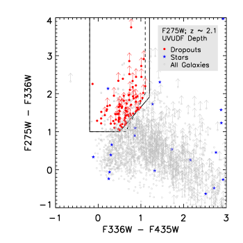
Figure 14.— (left panel) Color-color diagram illustrating F275W dropout candidates in UVUDF to ERS depth using the method of Hathi et al 2010 (H10). Colors are computed from subtracting magnitudes in the appropriate HST wavebands. Sources are illustrated to ERS depth (F336W = 26.5 AB) and have S/N degraded to match ERS observations (as discussed in the text). Colors and symbols are the same as in Figure 13. (right panel) Color-color diagram illustrating F275W dropout candidates to the full depth of UVUDF.

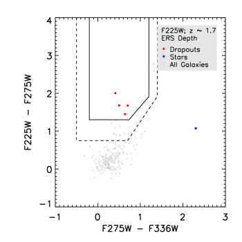
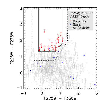
Figure 15.— (Top panel) Color-color diagram illustrating F225W dropout candidates in UVUDF to ERS depth using the method of Hathi et al 2010 (H10). Colors are computed from subtracting magnitudes in the appropriate HST wavebands. Sources are illustrated to ERS depth (F275W = 26.5 AB) and have S/N degraded to match ERS observations (as discussed in the text). Colors and symbols are the same as in Figure 13. (Bottom panel) Color-color diagram illustrating F225W dropout candidates to the full depth of UVUDF. Colors and symbols are the same as in the top panel. There are 25 F225W dropouts.

For a direct comparison with previous observations, we use the UVUDF data to examine source counts at the sensitivity of the shallower ERS data and reproduce the selection at the shallow sensitivity. Because the H10 and O10 dropout selection include a cut on source significance, we scale the S/N ratio of the UVUDF measurements to what we would expect from the ERS, using the HST Exposure Time Calculator (ETC). The S/N ratios change by factors of 0.19, 0.33, 0.33 for F336W, F275W, F225W respectively. The dropout selection at the shallower limit is also shown in the figures.

Table 3 indicates the number of dropout sources found using the methods of H10 and O10 in UVUDF data and, for comparison, those reported previously in ERS data. We find 37, 22, 4 H10 dropouts in F336W, F275W, F225W bands, respectively, to ERS depth in UVUDF, and we find 211, 88, 25 H10 dropouts in F336W, F275W, F225W bands, respectively, to the full depth in UVUDF. The raw number of dropouts in the narrow, deep UVUDF data is comparable to the numbers found in the wider, shallower ERS data. Table 3 also compares the sky densities of dropout candidates reported in H10 and O10 to those detected in UVUDF. We find dropout sources with comparable sky densities as H10 and O10 at the same depth and S/N limits.

Table 3 also compares the dropout selection methods of H10 and O10 applied in the UVUDF to each other; overall, the method of H10 is more conservative than the method of O10. For example, the number of O10 F336W dropouts and their resulting sky density exceeds the number of H10 F336W dropouts by a factor of 1.8 (67 O10 dropouts vs. 37 H10 dropouts). This disparity arises for several reasons. First, H10 uses a F435W-selected catalog, whereas O10 uses a F606W-selected catalog; therefore, O10 dropout selection begins with a larger sample of sources (531 F606W detected sources for O10 versus 391 F435W detected sources for H10). Second, H10 has a more stringent requirement for S/N in the bands blue-ward of the dropout band than O10 (S/N(F275W,225W) $<1$ for H10 vs. S/N(F275W,F225W) $<2$ for O10). Additional differences between the two methods include the upper S/N limit for sources in the dropout band adopted by H10 (S/N(F336W) $<3$ for H10 vs. no S/N(F336W) requirement for O10), the higher S/N requirement in the band redward of the dropout band in O10 (S/N(F435W) $>5$ for O10 vs. S/N(F435W) $>3$ for H10), and the differences in color selection regions between the two methods, as illustrated in Figure 13. Stars are found and rejected in each sample with approximately the same percentage (15% and 20% for H10 and O10 respectively).

6.1.2 Source Count Prediction

We use the published luminosity functions of H10 and O10 dropout sources to predict an expectation for the number of sources to be found in the UVUDF. Each luminosity function, expressed as a space density of galaxies, $\phi$, in units of Mpc^-3 mag^-1 as a function of absolute magnitude, $M$, at rest-frame 1500 Å is described by a Schechter function (Schechter, 1976). We use the fitted parameters $\phi_{*}$, $M_{*}$ and $\alpha$ reported in H10 and O10 for each dropout filter (F336W, F275W, F225W) to predict the space densities of galaxies in each redshift range.

The differential number of galaxies per unit redshift, dN/dz, for each dropout filter, is given by integrals over the Schechter luminosity function, $\Phi(M)$, expressed as a function of absolute magnitude, $M$, multiplied by the (published in H10 and O10) gaussian galaxy redshift distribution, g(z), and by the comoving volume element, $dV/dzd\Omega$, and finally integrated over the survey solid angle, $\Omega$.

$$\frac{dN}{dz}=\int d\Omega\int^{M_{lim}}_{-27}\frac{dV}{dzd\Omega}\Phi(M)g(z)dM$$ (4)

The lower limit of integration is chosen to include the brightest observable galaxies. The number of sources down to the magnitude limit, $M_{lim}$, is found by integration over the mean, $z_{m}$, of the galaxy redshift distribution within $\pm 1\sigma$ limits

$$N(<M_{lim})=\int^{z_{m}+\sigma}_{z_{m}-\sigma}\frac{dN}{dz}dz$$ (5)

No correction is made for completeness or selection efficiency effects (i.e. an effective volume correction), since these corrections are specific to each H10 and O10 data set, and are not transferrable to the UVUDF data.

The H10 and O10 luminosity functions were computed at rest-frame 1500 Å, which for F225W, F275W, F336W dropout galaxies at redshifts $z\sim 1.7,2.1,2.7$, correspond to observed-frame 4050, 4650, 5550 Å respectively. However, H10, O10 and the UVUDF catalogs are selected from different wavebands (e.g. UVUDF uses a $F435W$-selected catalog). To calculate the number density of LBGs, the upper magnitude limit for ERS and UVUDF were modified by color-correction terms. These terms account for the difference between rest-frame 1500 Å and the catalog detection band. An estimate of the upper magnitude limit at rest-frame 1500 Å is found by interpolating between the limits for the two closest photometric bands. These correction factors, $dm$, were added to the catalog detection limits, $m_{limit}$, to determine upper limits of integration for the luminosity functions, $m_{limit}=m_{detect}+dm$. For UVUDF data, we used a limit of $m_{detect}=28$ to avoid the magnitude range in which sources can be lost to CTI. Correction factors were found to be $dm=+0.130,-0.066,-0.236$ for F225W, F275W, F336W dropouts respectively.

For verification, we use the reported LF to predict the number counts that were observed in the ERS data themselves, the expected number counts in the UVUDF at a depth comparable to the shallower ERS data (at which the UVUDF is highly complete), and expected number counts in the UVUDF to its full depth. We note that the O10 and H10 LFs included substantial corrections for incompleteness, so we do not expect the number of galaxies predicted in the ERS to match the observations.

Predicted source counts for each selection method and dropout filter are presented in Table 3. In comparing the predictions to the observations, it is important to consider cosmic variance. For LBGs at these redshifts in fields the size of ERS and UDF, cosmic variance could be a large effect ($\sim$20-30%, bias=1.5, Somerville et al., 2004; Rafelski et al., 2009; Moster et al., 2011). However, in practice these fields are so close together on the sky (see Figure 4) that they are not independent in terms of large scale structure. In addition, we do not correct for incompleteness effects at the faint end of the UVUDF data. With these caveats in mind, we conclude that the predictions are generally consistent with the LBGs that we observe.

6.2. Resolving Galaxy Structure

The deep WFC3 UVIS data provide the depth and resolution that allow us to study star-forming regions at $z\sim 1$ in the rest-frame UV. We identified a sample of 179 galaxies with $m_{275}<27.5$ and $0.5<z_{phot}<1.5$, where photometric redshifts are taken from Rafelski et al. (2009). We find that galaxies frequently exhibit UV irregular morphologies and compact sizes (Figure 16), with a median effective radius of $0\farcs 19\pm 0\farcs 01$ ($1.5$ kpc at $z=1$) in the F275W filter. The F275W sizes are broadly consistent with those measured at rest-frame $\sim 4000$Å  which is probed by ACS I-band for $0.5\leq z<1$ and z-band for $1\leq z<1.5$. At these wavelengths, we find a median size of $0\farcs 18\pm 0\farcs 01$, suggesting that the recent star formation is occurring on the same spatial scale as previous generations of stars. However, when we deconstruct the galaxies clump-by-clump, clear morphological differences begin to emerge.

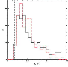
Figure 16.— Distribution of effective radii for galaxies in the UVUDF with $m_{275}<27.5$ and $0.5<z_{phot}<1.5$. We plot both the F275W (solid) and I-band (long-dashed) distributions, with the resolution limit marked with a vertical dashed line. Despite visible differences in the morphology between the rest-frame UV and rest-frame optical, the sizes remain approximately constant.

In Figure 17 we show some examples of $z\sim 1$ galaxies. The object in the second row is at $z_{\rm phot}=0.67$, where the F275W probes the light from short-lived O and B stars. In the UV, most of the light is concentrated in a few bright clumps. However, images at longer wavelengths (left column of Figure 17) reveal that these clumps are within the disk of a well defined spiral galaxy, with a clear bulge component at the center. If seen only in the UV, this object may resemble the clump-cluster galaxies observed at $z>2$ (e.g. Elmegreen et al., 2005), and predicted to form by fragmentation within gas rich disks (Ceverino et al., 2012). Clumps are predicted to migrate toward the center of the disk and coaelesce to form a bulge, which eventually should stabilize the disk (Dekel et al., 2009).

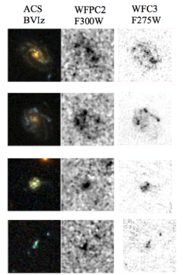
Figure 17.— HST gallery of clumpy spiral and irregular galaxies in the HUDF. (From left to right) Each panel shows (a) ACS BViz color combined image, UV WFPC2 F300W images from Voyer et al. (2009), and UV WFC3 F275W image of the combined Epoch 1 and 2. All images are 5″$\times$5″. Photometric redshifts of each galaxy from top to bottom are 0.63, 0.57, 0.77, 1.18.

UV-bright clumps were previously seen in the same object using WFPC2/F300W images (Voyer et al 2009), but the significantly higher resolution of the WFC3 UVIS data (WFPC2/F300W FWHM=0$\farcs$27 compared to the WFC3/F275W FWHM=0$\farcs$11), enables us to measure star-forming regions as small as $\sim$0.8 kpc (at $z=0.67$), reaching 8$\sigma$ above the background level. One of the clumps that is unresolved in the WFPC2 images is clearly resolved into two clumps with diameters of 1.0 kpc and 1.5 kpc in the WFC3 image. We have also identified clumps that do not appear to reside in a larger optical disk (bottom row Figure 17). This object is at $z_{\rm phot}=1.18$ and contains clumps with sizes ranging from $0.7-1.6$ kpc.

7. Summary

The UVUDF project obtained WFC3/UVIS observations of the Hubble Ultra Deep Field in three NUV filters, F225W, F275W, and F336W (Figure 1). The UDF was observed with each filter for a total of thirty orbits. The data were taken in three observing epochs with three orientation angles (Figure 3). The data in the first two epochs were taken with $2\times 2$ binning of the CCD readout in order to reduce the read noise that limited the sensitivity. For Epoch 3, as described in this paper (Section 3.1), the observing strategy was changed to use the WFC3 post-flash capability to add additional background to the observations in order to mitigate the degradation of the CCD charge transfer efficiency. The post-flashed data were taken without binning the CCD readout, because the additional background noise dominated the read noise. Coordinated parallel observations were obtained with ACS/WFC3 in order to provide very deep B-band fields, and the Epoch 3 parallels fall on top of one of the HUDF09 deep optical parallel fields (Figure 4).

The UVUDF observations present several data reduction challenges. The team has produced new calibration files for the binned data using binned and unbinned calibration observations obtained by STScI. In addition, we have reprocessed darks for all the data, modeling each dark’s gradient and using a more aggressive approach to flag hot and warm pixels (see Section 4.1).

The UVUDF data provide a stark demonstration of the effects of charge transfer inefficiency. In this paper, we provide evidence that CTI causes increased scatter in the photometry of sources far from the CCD readout (Figures 5, 6, and 7). The application of a statistical correction to the source flux densities based upon distance from readout is shown to reduce the scatter but not down to the level predicted from sky and read noise. We also find evidence that some faint sources far from the readout are lost to traps on the CCD in the data that were taken without post-flash (Figures 9, 10, and 11). We agree with the STScI recommendation that future WFC3 UVIS observations that require very sensitive measurements use the post-flash. The CTI also has demonstrated effects on the observed shapes of sources in the UVIS images, elongating them in the direction of the readout (Figure 8). This effect is problematic for both astrometric alignment and morphological analysis. STScI has released a preliminary version of software to apply a pixel-based correction for the CTI, but it will need significant testing and verification before it is stable enough to justify its use in producing enhanced science products for the archive.

The UVUDF data complete HST’s panchromatic coverage of the Hubble Ultra Deep Field. These data are applicable to a wide range of science topics. The measurement of the UV luminosity function, together with the mass function measured at longer wavelengths, will provide a statistical picture of the history of star formation during its peak epoch. The superb spatial resolution of UVIS will allow detailed analysis of star-forming “clumps” in galaxies, extending results obtained from optical images of $z\sim 2$ sources to later times and exploring the build up of normal galaxies. The UV sensitivity and spatial resolution will provide vital tests of the escape fraction of Lyman continuum photons from sources at $z<3$, and of the star formation rate efficiency of neutral atomic-dominated hydrogen gas at $z\sim 1-3$. Finally, the new UV measurements enable significant improvements in the estimation of photometric redshifts. These several science investigations will be presented by the UVUDF team in later papers.

In the current paper, we have presented a preliminary analysis of the galaxies observed in the UVUDF. We used the UVUDF data to select Lyman break galaxies at redshifts 1.7, 2.1, and 2.7. We find that the number density of dropouts is largely consistent with the number predicted by the published luminosity functions based on measurements in the ERS. In addition, we confirm that UVUDF images of clumpy galaxies at $z\sim 1$ have sufficient sensitivity and spatial resolution to support the planned analysis of the evolution of star-forming clumps.

There are many science uses for UV images of the UDF beyond those outlined above. This Treasury project will support a broad range of archival research. At the moment, we are limited by the need to continue characterizing and correcting the CTI effects. We expect that the CTI correction software will become stable in the coming year. When it has been robustly verified, we will produce enhanced science products to be distributed by the Mikulski Archive for Space Telescopes (MAST).

The UVUDF observations are currently the most sensitive component of a new generation of surveys that exploit the unique capabilities of WFC3/UVIS. The surveys will leave a legacy of UV imaging for use in a wide range of research. The next logical step in expanding HST’s UV legacy will be deep observations over a wider area than the UDF, in order to sample the variety of galaxy populations and their environments. These vital observations will greatly augment studies with the next generation of telescopes such as ALMA and JWST.

References

- Adelberger & Steidel (2000) Adelberger, K. L. & Steidel, C. C. 2000, ApJ, 544, 218
- Adelberger et al. (2004) Adelberger, K. L., Steidel, C. C., Shapley, A. E., Hunt, M. P., Erb, D. K., Reddy, N. A., & Pettini, M. 2004, ApJ, 607, 226
- Anderson (2013) Anderson, J. 2013, Instructions for Using the Alpha-Release of the WFC3/UVIS Pixel-based CTE Correction, Tech. rep., STScI
- Anderson & Bedin (2010) Anderson, J. & Bedin, L. R. 2010, PASP, 122, 1035
- Anderson et al. (2012) Anderson, J., MacKenty, J. W., Baggett, S., & Noeske, K. 2012, The Efficacy of Post-Flashing for Mitigating CTE-Losses in WFC3/UVIS Images, Tech. rep., STScI
- Balestra et al. (2010) Balestra, I., Mainieri, V., Popesso, P., Dickinson, M., Nonino, M., Rosati, P., Teimoorinia, H., Vanzella, E., et al. 2010, A&A, 512, 12
- Becker et al. (2007) Becker, A. C., Silvestri, N. M., Owen, R. E., Ivezić, Ž., & Lupton, R. H. 2007, PASP, 119, 1462
- Beckwith et al. (2006) Beckwith, S. V. W., Stiavelli, M., Koekemoer, A. M., Caldwell, J. A. R., Ferguson, H. C., Hook, R., Lucas, R. A., Bergeron, L. E., et al. 2006, AJ, 132, 1729
- Bertin & Arnouts (1996) Bertin, E. & Arnouts, S. 1996, A&AS, 117, 393
- Boissier et al. (2007) Boissier, S., Gil de Paz, A., Boselli, A., Madore, B. F., Buat, V., Cortese, L., Burgarella, D., Muñoz-Mateos, J. C., et al. 2007, ApJS, 173, 524
- Borders & Baggett (2009) Borders, T. & Baggett, S. 2009, WFC3 Instrument Science Report, 2009-16
- Bouwens et al. (2004) Bouwens, R. J., Illingworth, G. D., Blakeslee, J. P., Broadhurst, T. J., & Franx, M. 2004, arXiv
- Bouwens et al. (2006) Bouwens, R. J., Illingworth, G. D., Blakeslee, J. P., & Franx, M. 2006, ApJ, 653, 53
- Bouwens et al. (2012) Bouwens, R. J., Illingworth, G. D., Oesch, P. A., Franx, M., Labbé, I., Trenti, M., van Dokkum, P., Carollo, C. M., et al. 2012, ApJ, 754, 83
- Bouwens et al. (2011) Bouwens, R. J., Illingworth, G. D., Oesch, P. A., Labbé, I., Trenti, M., van Dokkum, P., Franx, M., Stiavelli, M., et al. 2011, ApJ, 737, 90
- Bouwens et al. (2010) Bouwens, R. J., Illingworth, G. D., Oesch, P. A., Stiavelli, M., Dokkum, P. v., Trenti, M., Magee, D., Labbé, I., et al. 2010, ApJ, 709, L133
- Bridge et al. (2010) Bridge, C. R., Teplitz, H. I., Siana, B., Scarlata, C., Conselice, C. J., Ferguson, H. C., Brown, T. M., Salvato, M., et al. 2010, ApJ, 720, 465
- Buat et al. (2010) Buat, V., Giovannoli, E., Burgarella, D., Altieri, B., Amblard, A., Arumugam, V., Aussel, H., Babbedge, T., et al. 2010, MNRAS, 409, L1
- Cawley et al. (2001) Cawley, L., Goudfrooij, P., Whitmore, B., & Stiavelli, M. 2001, Instrument Science Report WFC3, 2001-05
- Ceverino et al. (2012) Ceverino, D., Dekel, A., Mandelker, N., Bournaud, F., Burkert, A., Genzel, R., & Primack, J. 2012, MNRAS, 420, 3490
- Chen et al. (2002) Chen, H.-W., McCarthy, P. J., Marzke, R. O., Wilson, J., Carlberg, R. G., Firth, A. E., Persson, S. E., Sabbey, C. N., et al. 2002, ApJ, 570, 54
- Cimatti et al. (2008) Cimatti, A., Cassata, P., Pozzetti, L., Kurk, J., Mignoli, M., Renzini, A., Daddi, E., Bolzonella, M., et al. 2008, A&A, 482, 21
- Coe et al. (2006) Coe, D., Benítez, N., Sánchez, S. F., Jee, M., Bouwens, R., & Ford, H. 2006, AJ, 132, 926
- Coe et al. (2013) Coe, D., Zitrin, A., Carrasco, M., Shu, X., Zheng, W., Postman, M., Bradley, L., Koekemoer, A., et al. 2013, ApJ, 762, 32
- Daddi et al. (2010) Daddi, E., Bournaud, F., Walter, F., Dannerbauer, H., Carilli, C. L., Dickinson, M., Elbaz, D., Morrison, G. E., et al. 2010, ApJ, 713, 686
- Daddi et al. (2007) Daddi, E., Dickinson, M., Morrison, G., Chary, R., Cimatti, A., Elbaz, D., Frayer, D., Renzini, A., et al. 2007, ApJ, 670, 156
- Dekel et al. (2009) Dekel, A., Sari, R., & Ceverino, D. 2009, ApJ, 703, 785
- Dressler et al. (2012) Dressler, A., Spergel, D., Mountain, M., Postman, M., Elliott, E., Bendek, E., Bennett, D., Dalcanton, J., et al. 2012, arXiv, 7809
- Elbaz et al. (2011) Elbaz, D., Dickinson, M., Hwang, H. S., Díaz-Santos, T., Magdis, G., Magnelli, B., Le Borgne, D., Galliano, F., et al. 2011, A&A, 533, 119
- Ellis et al. (2013) Ellis, R. S., McLure, R. J., Dunlop, J. S., Robertson, B. E., Ono, Y., Schenker, M. A., Koekemoer, A., Bowler, R. A. A., et al. 2013, ApJ, 763, L7
- Elmegreen et al. (2008) Elmegreen, B. G., Bournaud, F., & Elmegreen, D. M. 2008, ApJ, 688, 67
- Elmegreen & Elmegreen (2005) Elmegreen, B. G. & Elmegreen, D. M. 2005, ApJ, 627, 632
- Elmegreen et al. (2005) Elmegreen, D. M., Elmegreen, B. G., & Ferguson, T. E. 2005, ApJ, 623, L71
- Feldmeier et al. (2002) Feldmeier, J. J., Mihos, J. C., Morrison, H. L., Rodney, S. A., & Harding, P. 2002, ApJ, 575, 779
- Finkelstein et al. (2012) Finkelstein, S. L., Papovich, C., Salmon, B., Finlator, K., Dickinson, M., Ferguson, H. C., Giavalisco, M., Koekemoer, A. M., et al. 2012, ApJ, 756, 164
- Ford et al. (2002) Ford, H. C., Illingworth, G. D., Clampin, M., et al. 2002, in Bulletin of the American Astronomical Society, Vol. 34, American Astronomical Society Meeting Abstracts #200, 675
- Fruchter & Hook (2002) Fruchter, A. S. & Hook, R. N. 2002, PASP, 114, 144
- Gardner et al. (2006) Gardner, J. P., Mather, J. C., Clampin, M., Doyon, R., Greenhouse, M. A., Hammel, H. B., Hutchings, J. B., Jakobsen, P., et al. 2006, Space Sci. Rev., 123, 485
- Gawiser et al. (2006) Gawiser, E., van Dokkum, P. G., Herrera, D., Maza, J., Castander, F. J., Infante, L., Lira, P., Quadri, R., et al. 2006, ApJS, 162, 1
- Genzel et al. (2008) Genzel, R., Burkert, A., Bouché, N., Cresci, G., Förster Schreiber, N. M., Shapley, A., Shapiro, K., Tacconi, L. J., et al. 2008, ApJ, 687, 59
- Giavalisco et al. (2004) Giavalisco, M., Ferguson, H. C., Koekemoer, A. M., Dickinson, M., Alexander, D. M., Bauer, F. E., Bergeron, J., Biagetti, C., et al. 2004, ApJ, 600, L93
- Gnedin & Kravtsov (2010) Gnedin, N. Y. & Kravtsov, A. V. 2010, ApJ, 714, 287
- Grogin et al. (2011) Grogin, N. A., Kocevski, D. D., Faber, S. M., Ferguson, H. C., Koekemoer, A. M., Riess, A. G., Acquaviva, V., Alexander, D. M., et al. 2011, ApJS, 197, 35
- Hathi et al. (2010) Hathi, N. P., Ryan, R. E. J., Cohen, S. H., Yan, H., Windhorst, R. A., McCarthy, P. J., O’Connell, R. W., Koekemoer, A. M., et al. 2010, ApJ, 720, 1708
- Iwata et al. (2009) Iwata, I., Inoue, A. K., Matsuda, Y., Furusawa, H., Hayashino, T., Kousai, K., Akiyama, M., Yamada, T., et al. 2009, ApJ, 692, 1287
- Kajisawa et al. (2006) Kajisawa, M., Konishi, M., Suzuki, R., Tokoku, C., Uchimoto, Y., Katsuno, Yoshikawa, T., Akiyama, M., et al. 2006, Publications of the Astronomical Society of Japan, 58, 951
- Kennicutt (1998a) Kennicutt, R. C. 1998a, ARA&A, 36, 189
- Kennicutt (1998b) —. 1998b, ApJ, 498, 541
- Kereš et al. (2009) Kereš, D., Katz, N., Fardal, M., Davé, R., & Weinberg, D. H. 2009, MNRAS, 395, 160
- Koekemoer et al. (2012) Koekemoer, A. M., Ellis, R. S., McLure, R. J., Dunlop, J. S., Robertson, B. E., Ono, Y., Schenker, M. A., Ouchi, M., et al. 2012, arXiv
- Koekemoer et al. (2011) Koekemoer, A. M., Faber, S. M., Ferguson, H. C., Grogin, N. A., Kocevski, D. D., Koo, D. C., Lai, K., Lotz, J. M., et al. 2011, ApJS, 197, 36
- Kron (1980) Kron, R. G. 1980, ApJS, 43, 305
- Kurczynski et al. (2012) Kurczynski, P., Gawiser, E., Huynh, M., Ivison, R. J., Treister, E., Smail, I., Blanc, G. A., Cardamone, C. N., et al. 2012, ApJ, 750, 117
- Kurk et al. (2013) Kurk, J., Cimatti, A., Daddi, E., Mignoli, M., Pozzetti, L., Dickinson, M., Bolzonella, M., Zamorani, G., et al. 2013, A&A, 549, 63
- Labbé et al. (2006) Labbé, I., Bouwens, R., Illingworth, G. D., & Franx, M. 2006, ApJ, 649, L67
- Labbé et al. (2003) Labbé, I., Franx, M., Rudnick, G., Schreiber, N. M. F., Rix, H.-W., Moorwood, A., van Dokkum, P. G., van der Werf, P., et al. 2003, AJ, 125, 1107
- Laureijs et al. (2012) Laureijs, R., Gondoin, P., Duvet, L., Saavedra Criado, G., Hoar, J., Amiaux, J., Auguères, J. L., Cole, R., et al. 2012, Space Telescopes and Instrumentation 2012: Optical, 8442
- Le Fèvre et al. (2005) Le Fèvre, O., Vettolani, G., Garilli, B., Tresse, L., Bottini, D., Le Brun, V., Maccagni, D., Picat, J. P., et al. 2005, A&A, 439, 845
- Lee et al. (2012a) Lee, K.-S., Alberts, S., Atlee, D., Dey, A., Pope, A., Jannuzi, B. T., Reddy, N., & Brown, M. J. I. 2012a, ApJ, 758, L31
- Lee et al. (2012b) Lee, K.-S., Ferguson, H. C., Wiklind, T., Dahlen, T., Dickinson, M. E., Giavalisco, M., Grogin, N., Papovich, C., et al. 2012b, ApJ, 752, 66
- MacKenty & Smith (2012) MacKenty, J. W. & Smith, L. 2012, CTE White Paper, Tech. rep., STScI
- Martel et al. (2008) Martel, A., Baggett, S., Bushouse, H., & Sabbi, E. 2008, Technical Instrument Report WFC3, 2008-01
- Massey (2010) Massey, R. 2010, MNRAS, 409, L109
- Massey et al. (2010) Massey, R., Stoughton, C., Leauthaud, A., Rhodes, J., Koekemoer, A., Ellis, R., & Shaghoulian, E. 2010, MNRAS, 401, 371
- Meurer et al. (1999) Meurer, G. R., Heckman, T. M., & Calzetti, D. 1999, ApJ, 521, 64
- Moster et al. (2011) Moster, B. P., Somerville, R. S., Newman, J. A., & Rix, H.-W. 2011, ApJ, 731, 113
- Nestor et al. (2013) Nestor, D. B., Shapley, A. E., Kornei, K. A., Steidel, C. C., & Siana, B. 2013, ApJ, 765, 47
- Noeske et al. (2012) Noeske, K., Baggett, S., Bushouse, H., Petro, L., Gilliland, R., & Khozurina-Platais, V. 2012, Instrument Science Report WFC3, 2012-09
- Nonino et al. (2009) Nonino, M., Dickinson, M., Rosati, P., Grazian, A., Reddy, N., Cristiani, S., Giavalisco, M., Kuntschner, H., et al. 2009, ApJS, 183, 244
- Oesch et al. (2010a) Oesch, P. A., Bouwens, R. J., Carollo, C. M., Illingworth, G. D., Magee, D., Trenti, M., Stiavelli, M., Franx, M., et al. 2010a, ApJ, 725, L150
- Oesch et al. (2010b) Oesch, P. A., Bouwens, R. J., Carollo, C. M., Illingworth, G. D., Trenti, M., Stiavelli, M., Magee, D., Labbé, I., et al. 2010b, ApJ, 709, L21
- Oesch et al. (2010c) Oesch, P. A., Bouwens, R. J., Illingworth, G. D., Carollo, C. M., Franx, M., Labbé, I., Magee, D., Stiavelli, M., et al. 2010c, ApJ, 709, L16
- Oesch et al. (2007) Oesch, P. A., Stiavelli, M., Carollo, C. M., Bergeron, L. E., Koekemoer, A. M., Lucas, R. A., Pavlovsky, C. M., Trenti, M., et al. 2007, ApJ, 671, 1212
- Overzier et al. (2011) Overzier, R. A., Heckman, T. M., Wang, J., Armus, L., Buat, V., Howell, J., Meurer, G., Seibert, M., et al. 2011, ApJ, 726, L7
- Pirzkal et al. (2005) Pirzkal, N., Sahu, K. C., Burgasser, A., Moustakas, L. A., Xu, C., Malhotra, S., Rhoads, J. E., Koekemoer, A. M., et al. 2005, ApJ, 622, 319
- Pirzkal et al. (2004) Pirzkal, N., Xu, C., Malhotra, S., Rhoads, J. E., Koekemoer, A. M., Moustakas, L. A., Walsh, J. R., Windhorst, R. A., et al. 2004, ApJS, 154, 501
- Popesso et al. (2009) Popesso, P., Dickinson, M., Nonino, M., Vanzella, E., Daddi, E., Fosbury, R. A. E., Kuntschner, H., Mainieri, V., et al. 2009, A&A, 494, 443
- Rafelski et al. (2011) Rafelski, M., Wolfe, A. M., & Chen, H.-W. 2011, ApJ, 736, 48
- Rafelski et al. (2009) Rafelski, M., Wolfe, A. M., Cooke, J., Chen, H.-W., Armandroff, T. E., & Wirth, G. D. 2009, ApJ, 703, 2033
- Rafelski et al. (2012) Rafelski, M., Wolfe, A. M., Prochaska, J. X., Neeleman, M., & Mendez, A. J. 2012, ApJ, 755, 89
- Ravindranath et al. (2006) Ravindranath, S., Giavalisco, M., Ferguson, H. C., Conselice, C., Katz, N., Weinberg, M., Lotz, J., Dickinson, M., et al. 2006, ApJ, 652, 963
- Reddy et al. (2012a) Reddy, N., Dickinson, M., Elbaz, D., Morrison, G., Giavalisco, M., Ivison, R., Papovich, C., Scott, D., et al. 2012a, ApJ, 744, 154
- Reddy et al. (2010) Reddy, N. A., Erb, D. K., Pettini, M., Steidel, C. C., & Shapley, A. E. 2010, ApJ, 712, 1070
- Reddy et al. (2012b) Reddy, N. A., Pettini, M., Steidel, C. C., Shapley, A. E., Erb, D. K., & Law, D. R. 2012b, ApJ, 754, 25
- Reddy & Steidel (2009) Reddy, N. A. & Steidel, C. C. 2009, ApJ, 692, 778
- Reddy et al. (2008) Reddy, N. A., Steidel, C. C., Pettini, M., Adelberger, K. L., Shapley, A. E., Erb, D. K., & Dickinson, M. 2008, ApJS, 175, 48
- Retzlaff et al. (2010) Retzlaff, J., Rosati, P., Dickinson, M., Vandame, B., Rité, C., Nonino, M., Cesarsky, C., & Team, T. G. 2010, A&A, 511, A50
- Rhodes et al. (2010) Rhodes, J., Leauthaud, A., Stoughton, C., Massey, R., Dawson, K., Kolbe, W., & Roe, N. 2010, PASP, 122, 439
- Rhodes et al. (2007) Rhodes, J. D., Massey, R. J., Albert, J., Collins, N., Ellis, R. S., Heymans, C., Gardner, J. P., Kneib, J.-P., et al. 2007, ApJS, 172, 203
- Riess & Mack (2004) Riess, A. & Mack, J. 2004, Instrument Science Report ACS, 2004-006
- Rix et al. (2004) Rix, H.-W., Barden, M., Beckwith, S. V. W., Bell, E. F., Borch, A., Caldwell, J. A. R., Haussler, B., Jahnke, K., et al. 2004, ApJS, 152, 163
- Rosati et al. (2002) Rosati, P., Tozzi, P., Giacconi, R., Gilli, R., Hasinger, G., Kewley, L., Mainieri, V., Nonino, M., et al. 2002, ApJ, 566, 667
- Sawicki & Thompson (2005) Sawicki, M. & Thompson, D. 2005, ApJ, 635, 100
- Scarlata et al. (2007) Scarlata, C., Carollo, C. M., Lilly, S. J., Feldmann, R., Kampczyk, P., Renzini, A., Cimatti, A., Halliday, C., et al. 2007, ApJS, 172, 494
- Schechter (1976) Schechter, P. 1976, ApJ, 203, 297
- Schmidt (1959) Schmidt, M. 1959, ApJ, 129, 243
- Shapley et al. (2006) Shapley, A. E., Steidel, C. C., Pettini, M., Adelberger, K. L., & Erb, D. K. 2006, ApJ, 651, 688
- Siana et al. (2009) Siana, B., Smail, I., Swinbank, A. M., Richard, J., Teplitz, H. I., Coppin, K. E. K., Ellis, R. S., Stark, D. P., et al. 2009, ApJ, 698, 1273
- Siana et al. (2007) Siana, B., Teplitz, H. I., Colbert, J., Ferguson, H. C., Dickinson, M., Brown, T. M., Conselice, C. J., de Mello, D. F., et al. 2007, ApJ, 668, 62
- Siana et al. (2010) Siana, B., Teplitz, H. I., Ferguson, H. C., Brown, T. M., Giavalisco, M., Dickinson, M., Chary, R.-R., de Mello, D. F., et al. 2010, ApJ, 723, 241
- Somerville et al. (2004) Somerville, R. S., Lee, K., Ferguson, H. C., Gardner, J. P., Moustakas, L. A., & Giavalisco, M. 2004, ApJ, 600, L171
- Steidel et al. (1999) Steidel, C. C., Adelberger, K. L., Giavalisco, M., Dickinson, M., & Pettini, M. 1999, ApJ, 519, 1
- Steidel et al. (2003) Steidel, C. C., Adelberger, K. L., Shapley, A. E., Pettini, M., Dickinson, M., & Giavalisco, M. 2003, ApJ, 592, 728
- Steidel et al. (1996a) Steidel, C. C., Giavalisco, M., Dickinson, M., & Adelberger, K. L. 1996a, AJ, 112, 352
- Steidel et al. (1996b) Steidel, C. C., Giavalisco, M., Pettini, M., Dickinson, M., & Adelberger, K. L. 1996b, ApJ, 462, L17
- Swinbank et al. (2009) Swinbank, A. M., Webb, T. M., Richard, J., Bower, R. G., Ellis, R. S., Illingworth, G., Jones, T., Kriek, M., et al. 2009, MNRAS, 400, 1121
- Szokoly et al. (2004) Szokoly, G. P., Bergeron, J., Hasinger, G., Lehmann, I., Kewley, L., Mainieri, V., Nonino, M., Rosati, P., et al. 2004, ApJS, 155, 271
- Teplitz et al. (2011) Teplitz, H. I., Chary, R., Elbaz, D., Dickinson, M., Bridge, C., Colbert, J., Le Floc’h, E., Frayer, D. T., et al. 2011, AJ, 141, 1
- Thilker et al. (2005) Thilker, D. A., Bianchi, L., Boissier, S., Gil de Paz, A., Madore, B. F., Martin, D. C., Meurer, G. R., Neff, S. G., et al. 2005, ApJ, 619, L79
- Thompson et al. (2005) Thompson, R. I., Illingworth, G., Bouwens, R., Dickinson, M., Eisenstein, D., Fan, X., Franx, M., Riess, A., et al. 2005, AJ, 130, 1
- van Dokkum et al. (2008) van Dokkum, P. G., Franx, M., Kriek, M., Holden, B., Illingworth, G. D., Magee, D., Bouwens, R., Marchesini, D., et al. 2008, ApJ, 677, L5
- Vanzella et al. (2008) Vanzella, E., Cristiani, S., Dickinson, M., Giavalisco, M., Kuntschner, H., Haase, J., Nonino, M., Rosati, P., et al. 2008, A&A, 478, 83
- Vanzella et al. (2005) Vanzella, E., Cristiani, S., Dickinson, M., Kuntschner, H., Moustakas, L. A., Nonino, M., Rosati, P., Stern, D., et al. 2005, A&A, 434, 53
- Vanzella et al. (2006) Vanzella, E., Cristiani, S., Dickinson, M., Kuntschner, H., Nonino, M., Rettura, A., Rosati, P., Vernet, J., et al. 2006, A&A, 454, 423
- Vanzella et al. (2009) Vanzella, E., Giavalisco, M., Dickinson, M., Cristiani, S., Nonino, M., Kuntschner, H., Popesso, P., Rosati, P., et al. 2009, ApJ, 695, 1163
- Vanzella et al. (2012) Vanzella, E., Guo, Y., Giavalisco, M., Grazian, A., Castellano, M., Cristiani, S., Dickinson, M., Fontana, A., et al. 2012, ApJ, 751, 70
- Voyer et al. (2009) Voyer, E. N., de Mello, D. F., Siana, B., Gardner, J. P., Quirk, C., & Teplitz, H. I. 2009, AJ, 138, 598
- Windhorst et al. (2011) Windhorst, R. A., Cohen, S. H., Hathi, N. P., McCarthy, P. J., Ryan, R. E., Yan, H., Baldry, I. K., Driver, S. P., et al. 2011, ApJS, 193, 27
- Wolfe & Chen (2006) Wolfe, A. M. & Chen, H.-W. 2006, ApJ, 652, 981
- Wolfe et al. (2005) Wolfe, A. M., Gawiser, E., & Prochaska, J. X. 2005, ARA&A, 43, 861
- Yan et al. (2004) Yan, H., Dickinson, M., Eisenhardt, P. R. M., Ferguson, H. C., Grogin, N. A., Paolillo, M., Chary, R.-R., Casertano, S., et al. 2004, ApJ, 616, 63