Evolution of Star Formation in the UKIDSS Ultra Deep Survey Field - I. Luminosity Functions and Cosmic Star Formation Rate out to z = 1.6

Abstract

We present new results on the cosmic star formation history in the SXDS-UDS field out to $z=1.6$. We compile narrow-band data from the Subaru Telescope and the Visible and Infrared Survey Telescope for Astronomy (VISTA) in conjunction with broad-band data from the SXDS and UDS, to make a selection of 5725 emission-line galaxies in 12 redshift slices, spanning 10 Gyr of cosmic time. We determine photometric redshifts for the sample using 11-band photometry, and use a spectroscopically confirmed subset to fine tune the resultant redshift distribution. We use the maximum-likelihood technique to determine luminosity functions in each redshift slice and model the selection effects inherent in any narrow-band selection statistically, to obviate the retrospective corrections ordinarily required. The deep narrow band data are sensitive to very low star formation rates (SFRs), and allow an accurate evaluation of the faint end slope of the Schechter function, $\alpha$. We find that $\alpha$ is particularly sensitive to the assumed faintest broadband magnitude of a galaxy capable of hosting an emission line, and propose that this limit should be empirically motivated. For this analysis we base our threshold on the limiting observed equivalent widths of emission lines in the local Universe. We compute the characteristic SFR of galaxies in each redshift slice, and the integrated SFR density, $\rho_{\rm{SFR}}$. We find our results to be in good agreement with the literature and parametrize the evolution of the SFR density as $\rho_{\rm{SFR}}\propto(1+z)^{4.58}$ confirming a steep decline in star formation activity since $z\sim 1.6$.

1 Introduction

A key goal and surmountable challenge for observational cosmology today is to assemble a reliable picture of the formation and evolution of galaxies, and the build up of stellar mass in the Universe. The secular evolution of galaxies is a result of the formation of new stars, and so understanding the processes triggering and truncating star formation in addition to placing constraints on the evolution of the star formation rate (SFR), in turn allows us to constrain theoretical models of galaxy formation and evolution. A multitude of star formation indicators have been utilized in evaluating the SFR, however each of these is subject to its own biases and caveats, in addition to the limitations technology places on the redshift range where each method is applicable.

Ultraviolet (UV) flux provides the most direct measurement of SFR by tracing hot young massive stars (e.g. Bunker et al. 2004, Ouchi et al. 2004, Arnouts et al. 2005, Baldry et al. 2005, Bouwens et al. 2010) however UV measurements are subject to large dust corrections and so carry a large uncertainty in addition to the danger of missing heavily obscured regions of star formation. The dust enshrouding young stars can itself be used to trace star formation, as it re-radiates the incident UV radiation in the infrared (e.g. Pérez-González et al. 2005, Le Floc’h et al. 2005). However, this method in turn struggles to detect some unobscured star formation. Less commonly used methods include using radio emission to trace supernova remnants associated with short-lived massive stars (e.g. Mauch & Sadler 2007) and tracing X-ray emission produced in X-ray binaries (of which one component is a massive O or B star). Alternatively, emission lines generated in H ii regions can be used to trace either the recombination of atoms or the forbidden lines that arise in this low-density environment. Emission lines in the optical and UV are of course subject to dust corrections much as many other tracers, however H$\alpha$ luminosity is particularly well calibrated for extinction effects.

The evolution of the star formation rate density, $\rho_{\rm{SFR}}$, is well studied, and a strong upward evolution is found with redshift out to $z\sim 1$ indicating that the peak of star formation activity occurs at $z>1$. The compilation of Hopkins & Beacom (2006) provides a broad overview of this relationship out to $z\sim 6$ but demonstrates that, even within the relatively well-constrained epoch, estimates of SFR evolution still vary according to indicator used. For instance the evolution of $\rho_{\rm{SFR}}$ is often parametrized as $\rho_{\rm{SFR}}\propto(1+z)^{\gamma}$, and in one of the earliest studies (using a rest frame UV colour to measure SFR) Lilly et al. (1996) found $\gamma=4$. However, their sample was hampered by a small survey area, and the larger UV-selected samples of e.g. Cowie et al. (1999), Wilson et al. (2002) and Prescott et al. (2009) found much shallower slopes of $\gamma=1.5,1.7\pm 1.0$ and $2.5\pm 0.3$ respectively. Meanwhile, the FIR luminosity found in Le Floc’h et al. (2005) translates to a $\gamma=3.2^{+0.7}_{-0.2}$.

Studies making use of continuum emission as a measure of the star formation activity of galaxies, whether it be UV emission, or its re-radiation in the infrared, allow us to quantify star formation in bright galaxies even down to low SFRs. The samples however are generally small, as sources not only require spectroscopy but must also be apparent in broad band filters in order to be detected — the imposed broad band flux limit means that samples in the optical become effectively stellar-mass limited, and therefore do not detect the lower mass population of galaxies responsible for an important contribution to the overall $\rho_{\rm{SFR}}$.

The use of narrow-band filters to detect emission-line galaxies provides a complementary technique to broad-band-selected samples. A narrow-band survey selects objects based on the strength of line emission, and so while the equivalent width of emission lines comes into play, samples are close to SFR-limited, allowing the analysis of SFR over a much broader range of stellar masses. Recently, many authors have utilised this technique to compile large samples of star-forming galaxies and examine the evolution of the SFR as traced by either H$\alpha$ luminosity (which scales directly with SFR; Kennicutt 1992) or alternatively the [O iii] and [O ii] forbidden lines which give a more loosely calibrated indication of the rate of star formation.

H$\alpha$ surveys have been hugely successful, from the pioneering work of Bunker et al. (1995) detecting only a handful of emitters, to the recent advances from the High Redshift Emission Line Survey (HiZELS; Geach et al. 2008, Sobral et al. 2009) that detected thousands of emission-line sources. Many authors have taken this approach, and the H$\alpha$ luminosity function is well-studied in a variety of environments (e.g. Gallego et al. 1995, Yan et al. 1999, Tresse et al. 2002, Fujita et al. 2003, Kodama et al. 2004, Umeda et al. 2004, Shioya et al. 2008 and Villar et al. 2008 to name but a few). Since infrared spectroscopy is required to trace the H$\alpha$ line beyond $z=0.4$, strong emission lines blueward of H$\alpha$ are required to study the higher redshift population using existing optical data sets. The [O ii] doublet for example has been traced to $z=1.6$ by Hogg et al. (1998), Hicks et al. (2002), Teplitz et al. (2003), Ajiki et al. (2003), Drozdovsky et al. (2005), Gilbank et al. (2010) and Ly et al. (2012).

Ly et al. (2012) incorporated the [O iii] tracer as well and derived luminosity functions in 11 redshift slices in the Subaru Deep Field based on H$\alpha$, [O iii] and [O ii] luminosities. Fitting a Schechter function to their data, they found strong evolution in the faint-end slope, $\alpha$, and the characteristic number density $\phi^{*}$, but little evolution in the characteristic luminosity of galaxies, L^∗. They interpreted these results as a comparatively stronger evolution of the low-luminosity galaxy population than those with higher intrinsic luminosities. They found a steep evolution in $\rho_{\rm{SFR}}$, in good agreement with previous results, a trend confirmed by the work of Sobral et al. (2013) who compiled the first view of star formation from $z=0.4$ out to $z=2.2$ using only H$\alpha$-selected galaxies. Sobral et al. (2013) parametrized the evolution in $\rho_{\rm{SFR}}$ as log $\rho_{\rm{SFR}}=-2.1/(z+1)$ suggesting a $\gamma\sim 3$ across the redshift range $0<z<1.6$. Conversely however, they found no evolution of $\alpha$, and set the parameter to $-1.6\pm 0.08$ for the last 11 Gyr, concluding that previous claims of evolution stemmed from heterogeneous samples. This value of $\alpha$ was in good agreement with Hayes et al. (2010) who found a slope of $\alpha=-1.72\pm 0.20$ at $z=2.2$ for an H$\alpha$-selected sample. Even consistently selected samples however (i.e. those using the same emission line to derive each luminosity function) still show discrepancies in the value of $\alpha$ and its evolution with redshift (or lack of). The H$\alpha$ emitters at $z=2.2$ found in Tadaki et al. (2011) for example result in a slope of $\alpha=-1.37$, much shallower than the studies of Hayes et al. (2010) and Sobral et al. (2013) and suggesting little evolution from high redshift to the present day. Hayes et al. (2010) however, while in agreement with a steep value of $\alpha$ argued that their results did indeed confirm an evolution in $\alpha$ compared to the shallower slope of $\alpha=-1.35$ at $z=0$ determined by Gallego et al. (1995). Evidently, values of $\alpha$ across redshift remain unclear, and tentative claims of the parameter’s evolution divide opinion further still. It is important therefore to better understand the factors which most affect the derivation of $\alpha$, in order to place more meaningful constraints on the faint end slope.

This paper demonstrates how the maximum likelihood method can be used to determine luminosity functions, and the benefits of this approach over existing methods. Narrow-band selection is inherently sensitive to only a certain region of parameter space, and retrospective corrections are ordinarily applied in order to account for the undetected objects. Here, we use a maximum likelihood analysis to model the selection effects statistically and robustly under assumptions about the underlying galaxy population. We explain in detail how we implement this method, and confirm the technique by replicating the results of Sobral et al. (2012) and Sobral et al. (2013).

Our luminosity functions are derived from narrow-band-selected emission-line galaxies in the Subaru/XMM-Newton Deep Field (SXDF), coincident with the Ultra Deep Survey (UDS) field of the UK Infrared Telescope (UKIRT)’s Infrared Deep Sky Survey (UKIDSS). We use the H$\alpha$, [O iii] and [O ii] emission lines to determine field luminosity functions in 12 redshift slices, spanning 10 Gyr of cosmic time, out to $z\sim 1.6$. We place constraints on the characteristic SFR in each redshift slice, and make estimates of $\rho_{\rm{SFR}}$ for comparison to values in the literature. The outline of this paper is as follows. In Section 2, we summarize the data used in this analysis, in Section 3 we discuss the source extraction and selection of narrow-band emitters, and present the colour–magnitude plots of narrow-band selected objects. Section 4 discusses our spectroscopically-confirmed subset, the star–galaxy separation technique applied in order to remove late-type stellar contaminants, our photometric redshift analysis and the resultant photometric redshift distributions, and finally our method of redshift slice assignment for emitters selected in each filter. Section 5 details our application of the maximum likelihood technique for determining luminosity functions, and discusses in detail the factors affecting the narrow-band selection technique. We describe also how this analysis carefully models the selection effects ordinarily corrected for retrospectively. In Section 6 we present luminosity functions (LFs) and derive the characteristic SFR and $\rho_{\rm{SFR}}$ in each redshift slice for comparison to literature results. Section 7 discusses the factors affecting our results and the effect of varying assumptions about the underlying galaxy population on the resultant values of $\alpha$. We summarize our conclusions in Section 8.

An H₀ = 70 kms^-1 Mpc^-1, $\Omega_{M}$ =0.3 and $\Omega_{\Lambda}$ =0.7 cosmology is assumed throughout, and all magnitudes are in the AB system.

2 Data

The data used (summarized in Table 1) are taken from the SXDF-UDS field in order to make use of the deep optical data from the Subaru/XMM-Newton Deep Survey (SXDS), in addition to deep infrared imaging from UKIDSS UDS.

Table 1: Summary of photometric data in all narrow and broad-band filters from Subaru, VISTA, CFHT, UKIRT and Spitzer.

Telescope:Instrument	Filter	Filter Type	Central wavelength	FWHM	5 sigma limit (2” aperture)	Citation
Subaru: Suprime-Cam	NB503	NB	5029Å	73Å	24.91	SXDS; Ouchi et al. (2008)
Subaru: Suprime-Cam	NB570	NB	5703Å	68Å	24.52	SXDS; Ouchi et al. (2008)
Subaru: Suprime-Cam	NB816	NB	8150Å	119Å	25.65	SXDS; Ouchi et al. (2008)
Subaru: Suprime-Cam	NB921	NB	9183Å	131Å	25.38	SXDS; Ouchi et al. (2009)
VISTA: VIRCAM	NB980	NB	9781Å	105Å	23.17	Jarvis et al., (in prep)
VISTA: VIRCAM	NB990	NB	9909Å	105Å	23.54	Jarvis et al., (in prep)
CFHT: Megacam	u	BB	3740Å	500Å	26.72	Foucaud et al., (in prep)
Subaru: Suprime-Cam	B	BB	4473Å	1079Å	27.39	Furusawa et al. (2008)
Subaru: Suprime-Cam	V	BB	5482Å	984Å	27.10	Furusawa et al. (2008)
Subaru: Suprime-Cam	R	BB	6531Å	1160Å	26.85	Furusawa et al. (2008)
Subaru: Suprime-Cam	i	BB	7695Å	1543Å	26.66	Furusawa et al. (2008)
Subaru: Suprime-Cam	z	BB	9149Å	1384Å	25.95	Furusawa et al. (2008)
UKIRT: WFCAM	J	BB	12500Å	1570Å	24.98	UKIDSS UDS; Almaini et al., (in prep)
UKIRT: WFCAM	H	BB	16500Å	2910Å	24.27	UKIDSS UDS; Almaini et al., (in prep)
UKIRT: WFCAM	K	BB	22000Å	3530Å	24.59	UKIDSS UDS; Almaini et al., (in prep)
Spitzer: IRAC	ch1	BB	35500Å	7411Å	23.55	Spitzer SpUDS: PI Dunlop
Spitzer: IRAC	ch2	BB	44900Å	10072Å	22.88	Spitzer SpUDS: PI Dunlop

The SXDS (Furusawa et al. 2008) covers 1.3 square degrees and delivers deep optical imaging in the B, V, R, i and z bands in five overlapping pointings of Suprime-Cam.

UKIDSS, comprised of 5 sub surveys of various areal coverages and depths (Lawrence et al., 2007) targeted the SXDF with the deepest of these surveys, the UDS (Foucaud et al. 2007, Almaini et al., [in prep]) covering 0.77 sq degrees. Here we utilise the Eighth Data Release (DR8) from this survey (details in Table 1). Additionally we incorporate u band data across the entire field from Megacam on the Canada France Hawaii Telescope (CFHT), and Spitzer IRAC imaging from the Spitzer-UDS (SpUDS) survey in channels 1 and 2.

Narrow-Band imaging was obtained from Suprime-Cam in four narrow-band filters, and smoothed using a Gaussian kernel to recover the same point spread function (PSF) as the broad-band optical data from Subaru (0.82 arcseconds). Details of these data can be found in Ouchi et al. (2008) and Ouchi et al. (2009).

In addition, we make use of two narrow-band filters on the Visible and Infrared Survey Telescope for Astronomy (VISTA). VISTA’s visible-infrared camera (VIRCAM; Dalton et al. 2006), is a wide-field near-IR camera consisting of sixteen 2048 $\times$ 2048 Raytheon VIRGO HgCdTe arrays distributed over the focal plane of VISTA. The paw-print of the 16 detectors provides a non-contiguous instantaneous field of view of 0.6 deg². Half of detector 16 is affected by a time-varying quantum efficiency which makes flat fielding that detector extremely challenging (see Jarvis et al. 2013 for further details). The NB980 and NB990 filters (Orr, Wallace and Dalton 2008) share a slot on VIRCAM — each covering eight detectors, and so to obtain a full pawprint from either of these filters the survey area has to be observed twice, with the instrument rotated 180 degrees. Consequently, the two VISTA NB images suffer from mismatched seeing in the top and bottom halves of the images, and so we smooth the data to the PSF of the worst-seeing parts of the VISTA pawprint (1.42 arcseconds).

In order to select a reliable sample with homogeneously determined photometric redshifts, we use only the region of sky covered by both SXDS and UDS imaging so as to provide 11 bands of photometry for every detection. The usable overlap of these deep broad-band surveys and the Subaru and VISTA narrow-band imaging data amounts to 0.63 sq degrees and 0.38 sq degrees respectively. The 6 narrow-band filters used for selection are shown together with Suprime-Cam broad-band filters across the corresponding wavelength ranges in Figure 1.

Figure 1: Wavelength coverage and transmission functions for all selection filters. Four narrow-band filters on Subaru, plus two on VISTA (bold black lines) together with broad-band filters at corresponding wavelengths also from the Subaru Telescope (dashed lines) are shown.

3 Sample Construction

We use the Source extraction software SExtractor (Bertin & Arnouts, 1996) to detect objects in each of the narrow-band (NB) images. SExtractor works by constructing a background map and then looking for groups of connected pixels above a threshold calculated from the root mean square (RMS) noise in the image. We require a group of 10 connected pixels at a significance of 1.5 times the background RMS to confirm a detection. We then estimate the narrow-band image depths by placing 10 000 randomly positioned 2-arcsecond apertures on each image and iteratively fitting a Gaussian to the sigma-clipped histogram of resultant fluxes. The catalogue is then cut to demand an NB-detection above 5$\sigma$ relative to our estimate of the sky noise in order for a source to be selected as a possible line emitter.

We make a very conservative area cut, dicarding first the official SXDS masked areas, and then visually inspecting the narrow-band images (with object detections overlaid) to discard additional areas of noisy coverage towards the edges of the CCD and then artifacts, areas around bright stars and CCD bleeds in the broad-band images. The areas removed from the study as a result of the visual inspection varied slightly from filter to filter.

3.1 Subaru Selection

For objects selected in one of the four Subaru NB filters, the sample was culled to the 5$\sigma$ limiting magnitude of the shallowest SXDS field. We next consider the interpolated broad-band colour at the wavelength of the selection filter as a measure of the continuum level for each object. We calculate this continuum (IntNB_cont) by interpolating between the two broad-bands adjacent to the NB assuming that continuum flux follows a power law:

$$\rm{IntNB}_{\rm\,cont}=\rm{BB1}-\rm{(BB1-BB2)}\,\frac{\log(\lambda_{\rm NB}/\lambda_{\rm BB1})}{\log(\lambda_{\rm BB2}/\lambda_{\rm BB1})}.$$ (1)

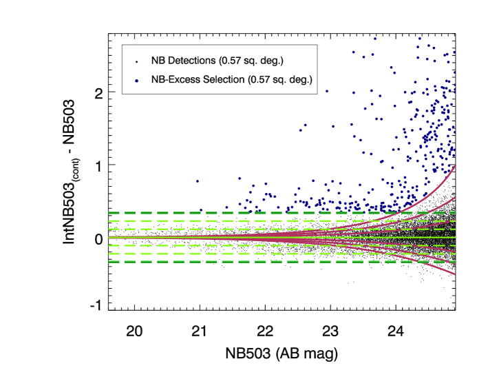
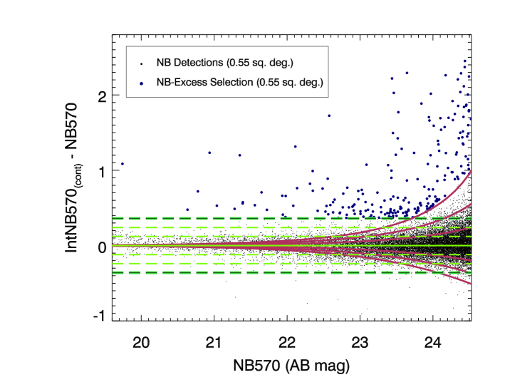
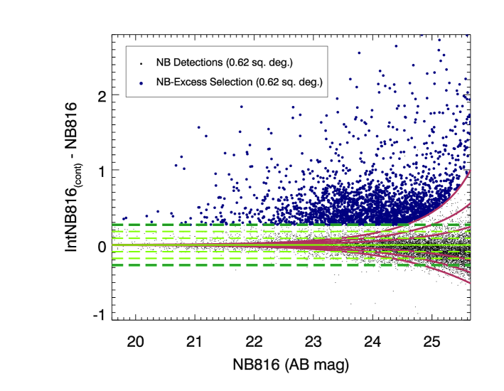
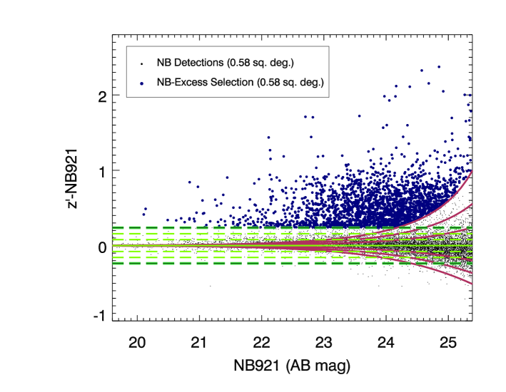
As filter NB921 lies centrally in the z-band, we calculate colour in this filter relative to the z-band only. Broad-band magnitudes are obtained by running SExtractor in dual image mode, and colours are measured in 2 arcsecond apertures. Objects are expected to scatter around zero in (IntNB${}_{\rm{cont}}-$NB), with emission-line sources showing a positive colour. In practice, the median colour of NB-selected sources is slightly offset from zero, due to the mismatch of interpolated broad-band magnitude and the true continuum magnitude at the wavelength of the NB. Furthermore, as we select objects across a broad range of NB magnitudes, we are essentially sampling different redshifts (in addition to different parts of the galaxy population) and so with changing NB-magnitude, we introduce a systematic error that gives rise to a gradient in the median colour of objects (typically of order $\sim 0.015$ mag). We remove the colour gradient by calculating the sigma-clipped median colour of sources as a linear function of NB mag, and subtracting this so that the resultant locus of colours lies along zero.

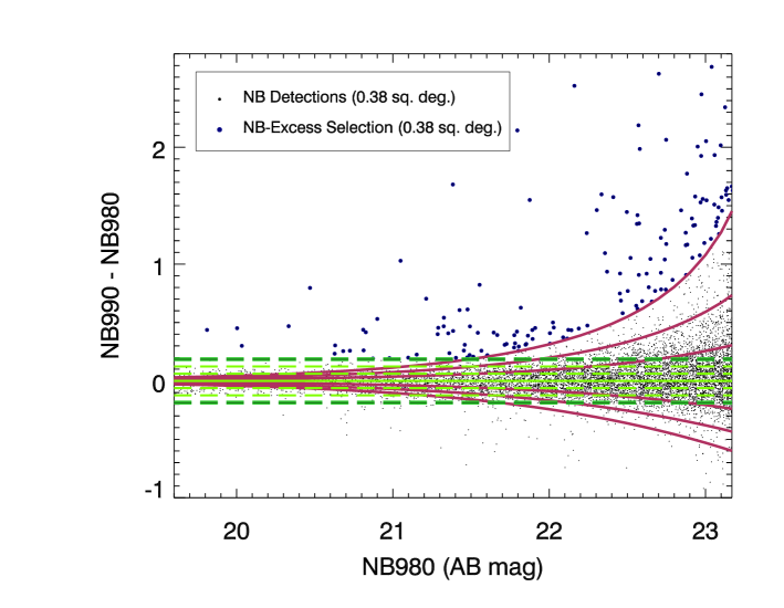
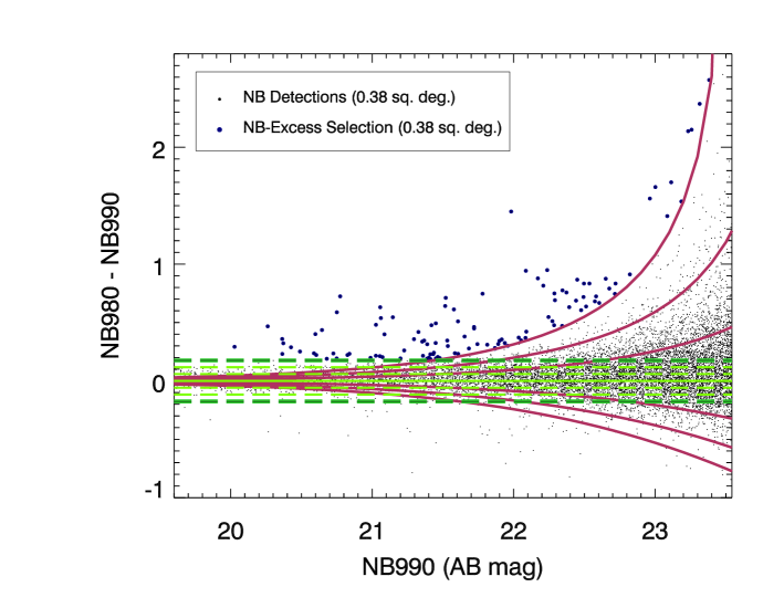
Potential emission-line objects must display an NB-excess of at least 3$\sigma$ relative to the sigma clipped median colour and 3$\sigma$ relative to the scatter from photometric uncertainty (in the relevant SXDS field) to be selected as an emitter. Photometric scatter is determined from the image depth estimates described above. Figure 2 shows colour-magnitude diagrams for each of the NB selections, with green lines showing the lines of 1, 2 and 3 $\sigma$ colour excess, and the red lines depicting the 1, 2 and 3 $\sigma$ photometric error trumpets.

We assume our observations are background limited, as even at the bright magnitudes where photon shot noise comes into play, colour scatter in (IntNB_cont-NB) is determined empirically and so the requirement of a 3$\sigma$ excess takes this scatter into account.

Figure 2: The colour–magnitude diagrams for the four Subaru narrow-band filters: NB503, NB570, NB816 and NB921, and the two VISTA narrow-band filters: NB980 and NB990. Detections are restricted to the 5$\sigma$ limiting NB-magnitude in the shallowest SXDS field. The solid green line depicts the median colour of sources (corrected for gradient and offset from zero — see text for details), dashed green lines show the 1, 2, and 3$\sigma$ limits on intrinsic colour scatter. Solid red lines depict the 1, 2, and 3$\sigma$ photometric errors respectively for the shallowest region of the five SXDS fields. Solid blue circles represent the entire sample of NB-excess-selected objects.

3.2 VISTA Selection

For selection in one of the two VISTA filters (seen alongside the Subaru filters in Figure 1), detections are made and NB-excesses evaluated following broadly the same method developed with the Subaru data. The only variation in the selection process is the manner in which we evaluate the continuum contribution to the NB measurement. The two VISTA NBs are close in wavelength, and so they sample objects at (effectively) the same point in their emission spectra; measured fluxes should therefore only differ significantly when an emission line is present in one of the two filters. This allows us to detect objects in one NB filter, and use photometry from the other as a measure of continuum flux for each object.

The double-NB selection technique circumvents the error introduced through inaccurate determination of interpolated broad-band colour (the main source of scatter introduced into the NB-broad-band colour) and so we anticipate the locus of VISTA-selected objects to be much tighter, allowing for a much less conservative 3$\sigma$ cut in colour scatter, i.e. a smaller colour-excess is now robust at the 3$\sigma$ level. Colour–magnitude diagrams for these two NBs are also shown in Figure 2 demonstrating the anticipated narrow locus, however the far shallower depth of the VISTA imaging results in a shallower sampling of the star-forming population.

Figure 3: BzK colour-colour diagrams for the two reddest filters in our Subaru NB-Excess selection; NB816 shown on the left and NB921 on the right. All objects falling below the solid black line are classed as stars according to Daddi et al. (2004). The subset of these objects that we identify as stars (and therefore eliminate from our analysis) are highlighted by red stars, yellow diamonds represent confirmed stars in the UDS. See main text for details.

4 Redshifts

Our narrow-band selection, spanning six NB filters from 5029 Å to 9909 Å  is sensitive to all the major diagnostic emission lines in the region from [O ii] to H$\alpha$ + [N ii], and samples redshift slices from z=0.14 ([O iii] in the NB570 filter) to z=1.6 where [O ii] falls in to the VISTA filters. With more than 7000 objects meeting the selection criteria, it is essential that we are able to reliably discriminate between the different lines falling in each filter while employing a technique suitable for dealing with such a volume of data. The combination of the deep SXDS-UDS imaging, and complementary u band and IRAC data, provides 11 broad bands of photometry available for every detection, allowing reliable determinations of objects’ spectral energy distributions (SEDs) and consequently accurate photometric redshifts. We have obtained spectra for a small subset of objects (discussed in Section 4.3) and use the redshifts derived as a training set for the photometric redshift code “EAzY” (Brammer, Van Dokkum and Coppi 2008).

4.1 Photometry

Photometry for the full selection of NB-excess selected objects is computed in all 11 broad bands using the iraf task phot in 2 arcsecond apertures. Astrometric corrections between Suprime-Cam data and the other images were performed using the method of Simpson et al. (2012). All Suprime-Cam imaging was reduced to provide a uniform PSF of $0.82$ arcsec, and the J, H and K band images from WFCAM are consistent with this to within $0.05$ arcsec, and so no corrections are applied to the measured photometry. B and K band images were smoothed using a Gaussian kernel to recover the same PSF as the u and IRAC images respectively, and fluxes from the u band image and the two IRAC images were then scaled according to the ratio of fluxes in the unsmoothed and smoothed images. All broad-band photometry is corrected for Galactic extinction of $A_{V}=0.070$ magnitudes (Schlegel et al., 1998) using the Cardelli, Clayton, & Mathis (1989) reddening law.

4.2 Star–Galaxy Separation

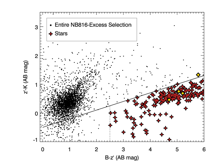
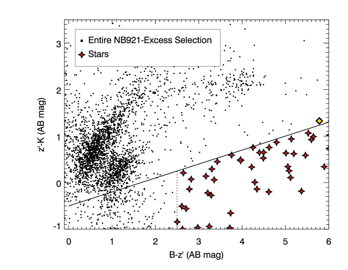
Our narrow-band-excess technique is inherently susceptible to the spurious selection of any object with a spectrum not well described by a power law. This leads to contamination of the sample by late-type stars which are known to exhibit very red, complex SEDs due to the many absorption features present in their spectra. We employ the two-colour BzK technique of Daddi et al. (2004) to identify and eliminate these stars from the red filters susceptible to this contamination. For the Subaru NB filters this applies to NB816 and NB921. Daddi et al., (2004) derive Equation 2, and class all objects below this line as stars.

$${(\emph{z}-\emph{K})<0.3\,(\emph{B}-\emph{z})-0.5}$$ (2)

As we are contaminated only by late-type, red, stars, we employ the additional criterion that objects must have B-z >2.5 to be classed as stars and eliminated from the selection.

The BzK colours of our sample are shown in Figure 3. The population of blue objects falling below the Daddi et al. (2004) BzK solid black line arises from scatter as a consequence of very faint K magnitudes ($>$ 26). We eliminate 256 stars in total, amounting to 2 per cent of the NB-excess sample.

Table 2: Detections per NB filter. Excess objects are defined as objects presenting an NB-excess above 3$\sigma$ in intrinsic colour scatter and photometric error. Galaxies are those objects that remain following the elimination of stars via our star–galaxy separation technique (see Section 4.2).

Filter	Detections	Excess Objects	Galaxies
NB503	43781	4368	4368
NB570	37846	1749	1749
NB816	97382	3816	3595
NB921	109126	5395	5360
NB980	16193	119	119
NB990	17755	191	191

Despite the red wavelength of the two VISTA filters, only NB990 is in danger of the spurious selection of stars due to the point in a late type star spectrum it samples. Running the NB990 selection through our BzK criteria however eliminates nothing from the small sample. Table 2 summarizes the number of detections in each filter plus numbers remaining in the sample after quantifying NB-excess and removing stars from the sample.

4.3 Spectroscopic Subset Analysis

With a preliminary selection of NB-excess objects in the central field of the SXDS, we compiled a target list for follow-up spectroscopy. Observations were carried out with the Inamori Magellan Areal Camera Spectrograph (IMACS) instrument on the Walter Baade Telescope on the dates of 2011 Jan 03-04, using 0.8 arcsecond slits and the 200 lines per mm grism (covering the wavelength range $\Delta\lambda=0.39-1.00\mu$m, giving $\Delta\lambda\sim 8$ Å pix^-1 at FWHM). The total exposure time was $335$ minutes, and seeing varied from $0.6-0.9$ arcseconds.

The spectra were reduced using the COSMOS reduction pipeline before extracting redshift information using the runz redshifting code (Saunders et al., 2004). We determine reliable redshifts for 129 of the sample, and assign 108 of these the highest quality flag. The remainder of the subset is made up of low signal to noise detections (where emission-line flux does not in fact meet our final criteria), spectra displaying a single unidentifiable line, spectra affected by cross-talk from other slits, and a small number of stars targeted to confirm our star–galaxy separation technique.

The modest but reliable subset of spectroscopic redshifts confirms that we are indeed selecting emission-line galaxies at the redshifts anticipated, and serves as a reference to determine the success of our photometric redshift technique applied to the rest of the sample.

4.4 Photometric Redshift Analysis

The default parameters of EAzY provide photometric redshifts in good agreement with the distribution expected for emission-line objects selected in these filters; however, to optimize the SED-fitting, we modify this default parameter set so as to minimize $\sigma_{\rm{NMAD}}$ for the spectroscopic subset (Equation 3; Brammer et al. 2008), where

$${\sigma_{\rm{NMAD}}=1.48\times{\rm{median}}\left(\left|\frac{\Delta z-{\rm{median}}(\Delta z)}{1+z_{\rm{spec}}}\right|\right).}$$ (3)

Figure 4: Comparison of spectroscopic and photometric redshifts for the subset of objects with spectroscopic follow-up, and spectroscopic redshifts of the highest quality flag. The bottom panel shows $z_{\rm{phot}}$ against $z_{\rm{spec}}$ for the optimized set of EAzY parameters. The top panel shows the distribution of $\Delta$z around zero. Cyan points represent our Magellan spectroscopic data, and black points represent all other available spectra in the UDS.

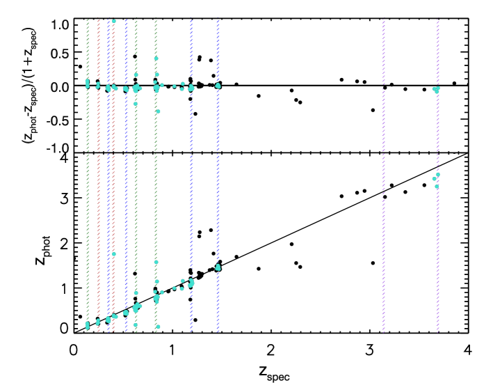
The number of catastrophic outliers ($>$ 5$\sigma$_NMAD) for definite spectroscopic redshifts (of the highest quality flag) equates to 5 per cent of the spectroscopic subset, with a value of $\sigma$${}_{\rm{NMAD}}=0.026$. Including objects with less certain spectroscopic redshifts raises this to 9 per cent. While photometric redshifts are commonplace for large survey data sets, particularly for K-selected (i.e. stellar-mass-limited) samples, photometry is frequently restricted to broad-bands only. Here we possess additional information that all objects remaining after the selection process must display a narrow-band excess at the wavelength of the filter.

While naïvely, we might interpret the presence of a narrow-band excess to mean that all sources must possess a major emission line redshifted to the wavelength of the selection filter, in practice the problem proves to be more complex. We design a pure emission-line template to investigate the effect of including narrow-band data in addition to broad-band photometry, before fine tuning the setup parameters. Our emission line template consists of the major emission lines Ly$\alpha$, [O ii], H$\beta$, [O iii], H$\alpha$ and [N ii] with negligible continuum flux. However, including this template now means that the complexities of the emission-line ratios come into play, along with the nature of the narrow-band excess. While the objects do indeed lie in distinct redshift slices, narrow-band excess can arise from a vast number of emission lines. We find that the inclusion of narrow-band data, along with an emission-line template, biases redshift determination towards the redshift slices associated with the emission lines in our template at the expense of a good fit to the broad-band photometry, thus adding redshift interlopers to our selection. The 11 bands of photometry are deep, and as EAzY is well equipped to determine redshifts based on this information alone we discard the narrow-band plus emission-line template setup at this stage.

We find the best agreement between $z_{\rm{phot}}$ and $z_{\rm{spec}}$ for the default template set, using broad-band data only (see Figure 4). This way redshifts are assigned independently of their detection method, allowing the correct identification of spectral breaks and additional better fitting emission lines than those included in the emission-line template. For the comparison in Figure 4 we also incorporate matches to the full set of spectra available in the UDS field. The larger SXDS–UDS spectroscopic sample (Simpson et al. 2012, and papers cited therein) includes many spectra that are the result of targeted follow-up of X-ray or radio sources, and is therefore heavily biased towards Active Galactic Nuclei (AGN). Objects with spectra from the larger sample (depicted by black dots in Figure 4) often appear at redshifts other than those typical for our selection, as they sample many objects with emission lines usually weak in star–forming galaxies.

4.5 AGN Contamination

We identify 8 (of the 129) objects as AGN according to the line-ratio diagrams of Lamareille (2010) or based on the presence of [Ne iii] emission. As we can use only our own spectroscopic follow-up from the Magellan telescopes to quantify AGN contamination in an unbiased manner, we infer a contamination fraction of 6${}^{+8.9}_{-3.9}$ percent. This correction is small and highly uncertain, and because AGN activity is undoubtedly associated with some star formation, removing these sources then leaves us susceptible to a possible over–correction and consequently an underestimate of star formation activity. We therefore choose not to correct our results for AGN contamination.

4.6 Resultant Photometric Redshift Distribution

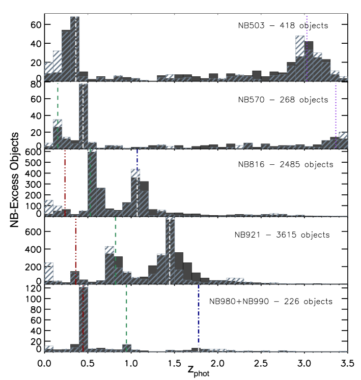
EAzY provides an output probability density distribution $P(z)$ for each object it evaluates. We use $z_{\rm{m2}}$, the redshift marginalized over the posterior redshift probability distribution (also taking into account the K-band apparent magnitude), to determine the redshift distribution of our objects and discriminate between the emission lines giving rise to narrow-band-excess. The resultant photometric redshift distribution can be seen in Figure 5. The advantage of the posterior redshift probability is two-fold: we combine the best estimate of redshift (using all SED templates) with a priori constraints on the likelihood of an object being at a particular redshift (given our knowledge of its colour and K magnitude prior), while taking into account the probability that the object lies at an alternative, less well-fit redshift. $z_{\rm{m2}}$ effectively provides a weighted mean, however the resultant distribution of redshifts and that for the best-fitting redshift ($z_{\rm{a}}$) are in fact very similar (traced by the two histograms in Figure 5), which demonstrates that we are not altering the best-fitting redshifts dramatically through marginalisation and use of the prior. We note that the small number of catastrophic outliers discussed in Section 4.4 produce doubly-peaked $P(z)$ distributions, with $z_{\rm{a}}$ often selecting a redshift of relatively small probability compared to the probability at the value of $z_{\rm{m2}}$. Similarly, the small peaks of objects lying at $z_{\rm{a}}$=0 are the result of objects missing a red band of photometry and producing a small peak at $z_{\rm{a}}$=0 in their $P(z)$ distributions. This lends further support to the advantages of $z_{\rm{m2}}$ which in these cases avoids the small $z_{\rm{a}}$=0 spike via the weighted mean. Figure 5 shows that we are selecting emission-line galaxies at the anticipated redshifts and highlights the peaks in the distribution associated with H$\alpha$, [O iii] and [O ii], in addition to Ly$\alpha$ in the two bluest filters (Ouchi et al. 2008; not included in this analysis).

The lowest panel of Figure 5 shows the combined data sets of NB980 and NB990. As these two filters are very close in wavelength ($\Delta\,\lambda_{c}$ $\sim$120Å) we choose to combine the two data sets to combat the small number of detections (with a 5$\sigma$ detection cutoff in the shallowest filter; NB980). The NB980 and NB990 data sets are evaluated separately, and then combined before assigning objects to a redshift slice. The combined data set (hereafter NB985) is treated as a single selection from here on.

Figure 5: Photometric redshift distributions for the 4 Subaru narrow-band filters and the combined distributions from VISTA’s NB980 and NB990 filters. The dark grey filled histogram represents $z_{\rm{m2}}$, the redshift marginalized over the posterior redshift probability distribution, and the light grey hatched histogram traces $z_{\rm{a}}$, the best fit redshift. Panels top to bottom: NB503, NB570, NB816, NB921 and NB980+NB990 in redshift bins of width $\Delta z$= 0.1. Vertical lines indicate the redshifts at which different emission lines would be detected in the various filters: triple-dot-dashed lines show H$\alpha$ (dark red), dashed lines the [O iii] doublet and H$\beta$ (green), and dot-dashed lines [O ii] in blue. Filters NB503 and NB570 also show peaks at z$\sim$3 where we detect Ly$\alpha$ (dotted purple line).

4.7 Redshift Slice Assignment

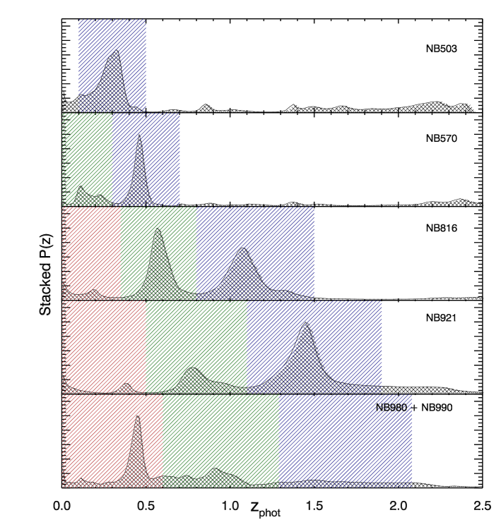
Before assigning objects to a particular redshift slice we consider the stack of $P(z)$ values for each NB-selection of objects (seen in Figure 6). We bin objects into the redshift slices associated with the peaks in the data, and assign the upper and lower limits of the bins according to the minima in the stacked $P(z)$ distribution. For the VISTA selection where the minima of the distribution are less apparent, the widths of the NB921 redshift windows are applied, centred on the peaks of the VISTA data. Table 3 summarizes the final numbers of objects in each redshift slice and the redshift ranges over which each peak was defined.

Table 3: Number of objects assigned to each redshift slice. The redshift range quoted refers to the limits in $z_{\rm{m2}}$ according to which objects were binned into redshift slices. These limits are taken from the minima in Figure 6 with the exception of the VISTA data for which the NB921 limits were transposed to the appropriate redshift. The number of objects per slice is the number of real objects assigned to a redshift slice from our catalogue, that were used to derive a luminosity function for this redshift range.

Filter	Redshift	Line	Objects
NB503	0.10 $<$ 0.35 $<$ 0.50	[O ii]	142
NB570	0.00 $<$ 0.14 $<$ 0.30	[O iii]	42
NB570	0.30 $<$ 0.53 $<$ 0.70	[O ii]	96
NB816	0.00 $<$ 0.25 $<$ 0.35	H$\alpha$	152
NB816	0.35 $<$ 0.63 $<$ 0.80	[O iii]	985
NB816	0.80 $<$ 1.19 $<$ 1.50	[O ii]	1013
NB921	0.00 $<$ 0.40 $<$ 0.50	H$\alpha$	279
NB921	0.50 $<$ 0.83 $<$ 1.10	[O iii]	930
NB921	1.10 $<$ 1.46 $<$ 1.90	[O ii]	2204
NB985	0.00 $<$ 0.50 $<$ 0.60	H$\alpha$	153
NB985	0.60 $<$ 0.99 $<$ 1.29	[O iii]	33
NB985	1.29 $<$ 1.64 $<$ 2.08	[O ii]	23

Figure 6: Stacked probability density distributions for each NB-selection of objects, shown over the redshift range relevant for this study. Red (H$\alpha$), green ([O iii]) and blue ([O ii]) shaded regions represent the redshift ranges assigned to a slice for a particular filter/line combination.

4.8 Line fluxes

Narrow-Band selections are by necessity made in an observable parameter space, here based on line flux. Apparent aperture line fluxes (hereafter: line fluxes) for objects in each redshift slice are derived from the initial SExtractor detection measurements. The entirety of the NB-excess is assumed to arise from an emission line and so line flux ($\mu$Jy) is computed as Equation 4, and converted to Wm^-2.

$${{\rm{Line\>flux}}={\rm{flux_{NB}}}-{\rm{flux_{cont}}}}$$ (4)

where flux_NB is the flux in the narrow-band, and flux_cont is the continuum contribution to that narrow-band flux.

Figure 7: Line transmission for NB921. Panels from left to right show the effective line transmission with redshift for H$\alpha$, [O iii] and [O ii] respectively, as a synthetic spectrum is propagated through the NB921 filter.

5 Maximum Likelihood Luminosity Functions

We employ the maximum likelihood method of Marshall et al. (1983) in order to fit luminosity functions to the data. We assume the distribution of line luminosities in a given redshift slice will follow a Schechter function, given in log form by Equation 5:

$${\phi\,(L)\,{\rm{dlog}}L={\rm{ln10}}\,\phi^{*}\left(\frac{L}{L^{*}}\right)^{\alpha+1}\,e^{-({L}/{L^{*}})}\,{\rm{dlog}}L}$$ (5)

where $\phi$^∗, $L^{*}$ and $\alpha$ are the characteristic number density, characteristic luminosity, and the gradient of the faint-end slope respectively (Schechter, 1976). We assume negligible cosmic evolution across the small redshift interval per slice. Next we consider how the distribution of true line luminosities maps onto our observed distribution of line fluxes.

Splitting the line flux range where we are sensitive to lines into bins small enough to expect no more than 1 object per bin, we can write the likelihood of finding an object in bins F_i and no objects in bins F_j, as Equation 6 for a given luminosity function:

$${{\Lambda}={\prod_{F_{i}}}\Psi(F_{i})\,{\rm{dlog}}F\,e^{-\Psi(F_{i}){\rm{dlog}}F}\prod_{F_{j}}\,e^{-\Psi(F_{j}){\rm{dlog}}F}}$$ (6)

where $\Psi(F_{i})$ is the probability of detecting an object with line flux between $F$ and $10^{{\rm{dlog}}F}F$. This simplifies to Equation 7, where F_k is the product over all bins:

$${{\Lambda}={\prod_{F_{i}}\Psi(F_{i})\,{\rm{dlog}}F\,\prod_{F_{k}}\,e^{-\Psi(F_{k}){\rm{dlog}}F}}}$$ (7)

We then define the likelihood function as $S=-2{\rm{ln}}\Lambda$ and minimize this (Equation 8) in order to determine the parameters of the model ($\phi$^∗, $L^{*}$, $\alpha$) that best reproduce the observed data.

$${{S}={-2\sum}\,{\rm{ln}}\Psi(F_{i})+2\int\Psi(F)\,{\rm{dlog}}F}$$ (8)

To obtain $\Psi\,(F)$ (the observed line luminosity function) from $\phi\,(L)$ (the true line luminosity function) we must consider the selection effects imposed in observing the data and statistically model these perturbations to $\phi\,(L)$ before minimising the likelihood function.

5.1 Treatment of the filter profile

To produce a LF, we must first assess the NB filter response for the emission line of interest as a function of redshift. A given line flux may arise from a line near the centre of of a detection filter, or an intrinsically brighter line lying closer to the edge of the filter where transmission is lower.

We define $T(z)$, the relative transmission with redshift, to determine the redshift range to which each filter/line combination is sensitive, accounting for filter transmission in addition to contributions from other lines. $T(z)$ is calculated by propagating a synthetic spectrum through the filter transmission curve (an example of the resultant line transmission is seen in Figure 7), using standard line ratios ([N ii]/H$\alpha$=0.33, [O iii]/H$\beta$ = 3, [O ii] in the low density limit; Osterbrock & Ferland 2006) normalized to the line of interest. $F$, our line flux, now becomes:

$${F=\left(\frac{L}{4\pi d_{l}^{2}(z)}\right)T(z)}$$ (9)

where $L/4\pi d_{l}^{2}(z)$ is the true flux, convolved with filter transmission $T(z)$. $\Psi(F)$, the probability of seeing a line of flux $F$, now becomes:

$${\Psi(F){\rm{dlog}}F=\int\phi\left(\frac{4\pi d_{l}^{2}(z)F}{T(z)}\right)\,\left(\frac{{\rm{d}}V}{{\rm{d}}z}\right)\,{\rm{d}}z\,{\rm{dlog}}L}$$ (10)

where ${\rm{d}}V/{\rm{d}}z$ is the co-moving volume interval in our field per unit redshift, and the integral is performed over the redshift range to which the filter is sensitive.

5.2 Line detectability

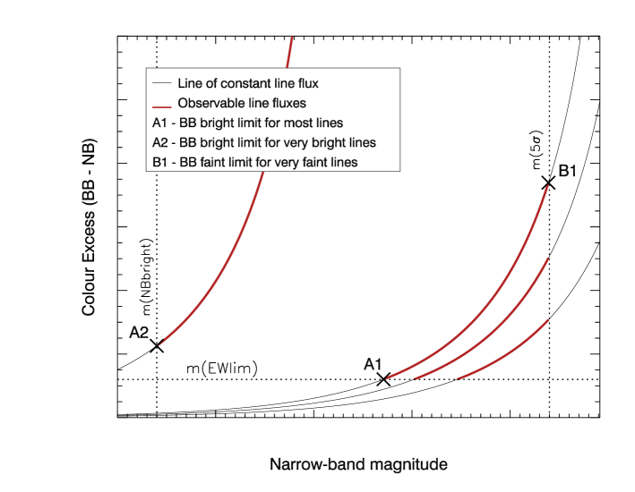
The detection of an emission line in our study requires it to reside in an observable part of parameter space in the NB magnitude – colour-excess plane. i.e. the region within the three dotted lines in Figure 8. The detection fraction as a function of line flux, is then given by Equation 11:

$${f_{{\rm{det}}}(F)=\frac{\int^{m_{\rm faint\ limit}}_{m_{\rm bright\ limit}}\phi_{\rm{BB}}(m_{\rm{BB}}){\rm{d}}m_{\rm{BB}}}{\int^{m_{\rm{faint}}}_{-\infty}\phi_{\rm{BB}}(m_{\rm{BB}}){\rm{d}}m_{\rm{BB}}}}$$ (11)

where $\phi_{\rm{BB}}(m_{\rm{BB}})$ is a Schechter fit to the interpolated broad-band magnitudes of all galaxies within a particular filter’s redshift range, and is derived from the photometric redshift catalogue of Grützbauch et al. (2011). The numerator of ${f_{\rm{det}}}$ denotes the sample of galaxies our technique is capable of detecting (thick red lines in Figure 8), and the denominator denotes the entire population of galaxies capable of hosting the line down to some integration limit, ${m_{\rm{faint}}}$. ${m_{\rm{faint}}}$ is the assumed faintest magnitude of a galaxy capable of hosting a particular emission line luminosity. Different authors set this limit differently and somewhat arbitrarily. Here we adopt a limit based on the rest frame equivalent width of the line of interest seen in the local Universe, and set EW${}_{m_{\rm{faint}}}$$=100$Å  (Kennicutt, 1992). The resultant Schechter fit to our observed line fluxes is sensitive to the integration limit of the denominator (${m_{\rm{faint}}}$). The effect of varying this limit is discussed in Section 7.2.

The limits of integration for the numerator are somewhat more complex. The detection of a galaxy of particular broad-band magnitude for a line of particular line flux is limited at the bright end by the fainter of 2 broad-band magnitudes: either that corresponding to the EW limit, or that corresponding to the bright NB limit. At the faint end, broad-band magnitude is limited by the brighter of two broad-band magnitudes: that corresponding to the 5$\sigma$ NB detection limit, or that corresponding to the faintest broad-band magnitude capable of hosting a line of this line flux (i.e. ${m_{\rm{faint}}}$). Figure 8 illustrates the location of the bright and faint broad-band limits in relation to lines of constant line flux.

5.2.1 Broad-band magnitude bright limit

For the majority of lines the bright limit is set by m_EWlim (depicted as point A1 in Figure 8) and can be understood by considering our selection criteria. For an object to be included in our analysis it must display a colour excess of at least 3$\sigma$ significance. At bright magnitudes (where intrinsic colour–scatter dominates uncertainty) detections are limited by an equivalent width limit (dotted horizontal line in Figure 8). Therefore, for a given line flux, only host galaxies fainter than a particular broad-band magnitude will result in an equivalent width large enough to be selected in our sample.

For very bright lines however (such as that traced on the left hand side of Figure 8) the limiting factor becomes the saturation limit for point sources in the broad-band imaging used to determine narrow-band excess. Very bright lines (of flux greater than this) will not be selected. The value of this limit varies from filter to filter, and we define each limit as the point at which the locus of stellar objects crosses the $3\sigma$ color–excess line. Brighter than this limit, emission-line objects could be indistinguishable from stellar objects. The broad-band saturation limits for each NB filter are as follows: NB503=19.0, NB570=19.1, NB816=19.25, NB921=19.2, NB980/NB990=16.0. We note that the effect of this limit is small, indeed removing this correction from the analysis altogether and integrating Equation 8 to infinite flux has no effect above $z\sim 0.6$, and very little effect below this. An example of a particularly bright line (of 60 $\sigma$ significance) is shown in Figure 8 depicted by the line on the far left. This demonstrates how only lines of very large line flux are limited by this saturation limit (point A2 in Figure 8) as opposed to the EW limit (A1).

5.2.2 Broad-band magnitude faint limit

The faint limit for the majority of lines is set by ${m_{\rm{faint}}}$, i.e. the true limiting magnitude of the population of galaxies capable of hosting that line, as detailed above.

For exceptionally faint lines however, the detection limit of our catalogue comes into play. For an object to be detected its broad-band magnitude must be bright enough that when added to its line flux its NB magnitude is above the 5$\sigma$ detection threshold, and so for very faint lines this constraint sets the faint limit on broad-band magnitude. Point B1 represents this limit for a particular line flux in Figure 8.

Figure 8: Lines of constant line flux in the NBmag - (colour-excess) plane. The dotted lines represent the limiting equivalent width for an emission line to meet the selection criteria, and the faintest broad-band magnitude that when combined with a given line flux will meet the 5 $\sigma$ narrow-band threshold. A and B represent points on a line of constant line flux that correspond to the bright and faint broad-band limiting magnitudes respectively. Thick red lines highlight the portion of each line of constant line flux that is detectable in our sample.

Equation 11 then becomes Equation 12:

$${f_{{\rm{det}}}(F)=\frac{\int^{\rm min(m_{5\sigma},m_{\rm faint})}_{\rm max(m_{\rm{EWlim}},m_{\rm NBbright})}\phi_{\rm{BB}}(m_{\rm{BB}}){\rm{d}}m_{\rm{BB}}}{\int^{m_{\rm{faint}}}_{-\infty}\phi_{\rm{BB}}(m_{\rm{BB}}){\rm{d}}m_{\rm{BB}}}}$$ (12)

and $\Psi(F)$ now takes its final form:

$${\Psi(F)\,{\rm{dlog}}\,F=f_{\rm{det}}\,(F)\int\phi\left(\frac{4\pi d^{2}_{l}F}{T(z)}\right)\frac{{\rm{d}}V}{{\rm{d}}z}\,{\rm{d}}z\,{\rm{dlog}}\,F.}$$ (13)

We note that the presence of a strong correlation between SFR and stellar mass (e.g. Noeske 2008, however see Sobral et al. 2011 for an alternative view) would mean that low–luminosity lines would be less likely to be found in more massive galaxies. We will address this issue and its effect on line detectability in paper 2, where we will study luminosity functions as a function of stellar mass.

5.3 Detection Completeness

Finally, we assess the detection completeness of the narrow-band selection catalogue retrieved via SExtractor. The completeness of detections is dependent on the depth of the detection image and on the size of the aperture used. As our analysis is carried out in 2 arcsecond apertures and a retrospective aperture correction applied (see below), we assess completeness in the same manner down to the 5$\sigma$ limiting magnitude. We construct a series of images inserting randomly positioned fake point sources in each image, allowing us to determine recovery fraction as a function of magnitude. We estimate incompleteness per $\Delta$m${}_{{\rm{NB}}}=0.05$ bin, and create an appropriate number of sources with NB excesses distributed following the observed distribution of detected objects, and with NB magnitudes uniformly distributed within the bin. The effect is small as we only populate the faintest bins, typically adding fewer than 10 objects to a LF. This number rises to 21 objects (a 2 per cent increase) for the second most densely populated LF ([O ii] in NB816) and 91 objects (a 4 per cent increase) for [O ii] in NB921 where the number of detections is more than a factor of 2 larger again. Corrections are particularly low due to the stringent $5\sigma$ NB-detection requirement.

5.4 Galactic Extinction and Aperture Correction

Each LF is corrected for Galactic extinction of $A_{V}=0.070$ magnitudes using the Cardelli et al. (1989) reddening law (following the same method as in Section 4.1). As the analysis is carried out using aperture photometry, we must assess the fraction of flux that is lost by only considering the light within our 2 arcsecond aperture. We calculate the ratio of total NB flux to aperture NB flux using the output SExtractor values (flux_best and flux_aper respectively) for each redshift slice, and scale each output LF according to the median ratio in that slice. The correction is typically small (a factor of $\sim$ 1.2) even at the lowest redshifts, however for the smoothed VISTA NB data we find a slightly larger correction ($\sim$ 1.8) due to a much broader PSF.

6 Results

We derive luminosity functions to examine the evolution of the H$\alpha$, [O iii] and [O ii] luminosity functions. The resultant Schechter fits provide LFs in 12 redshift slices between 0.14 and 1.64. Using the parametrizations of these LFs we can derive SFRs and compute $\rho_{\rm{SFR}}$ to examine the evolution of star formation with redshift.

6.1 Luminosity Functions

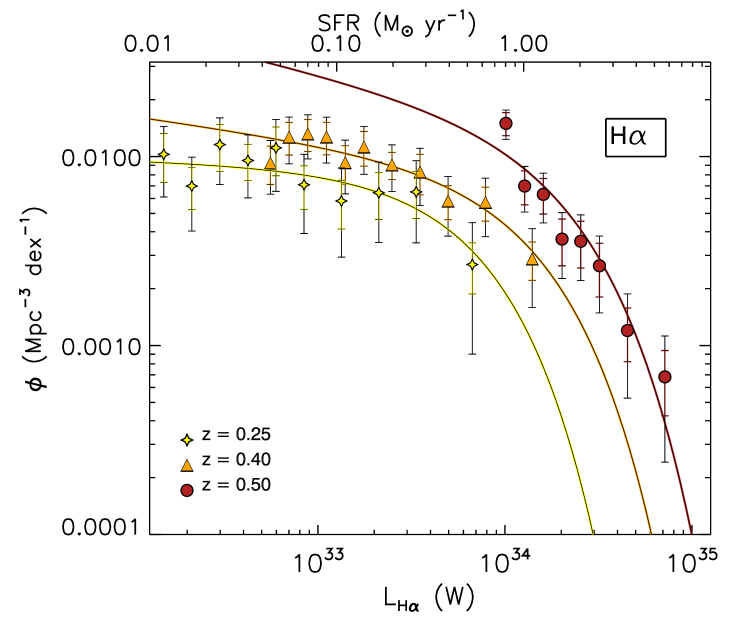
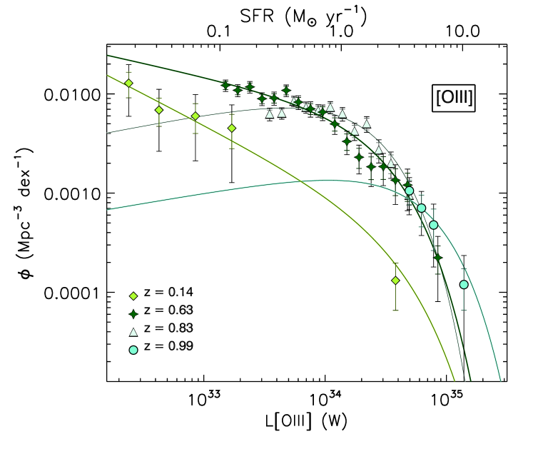
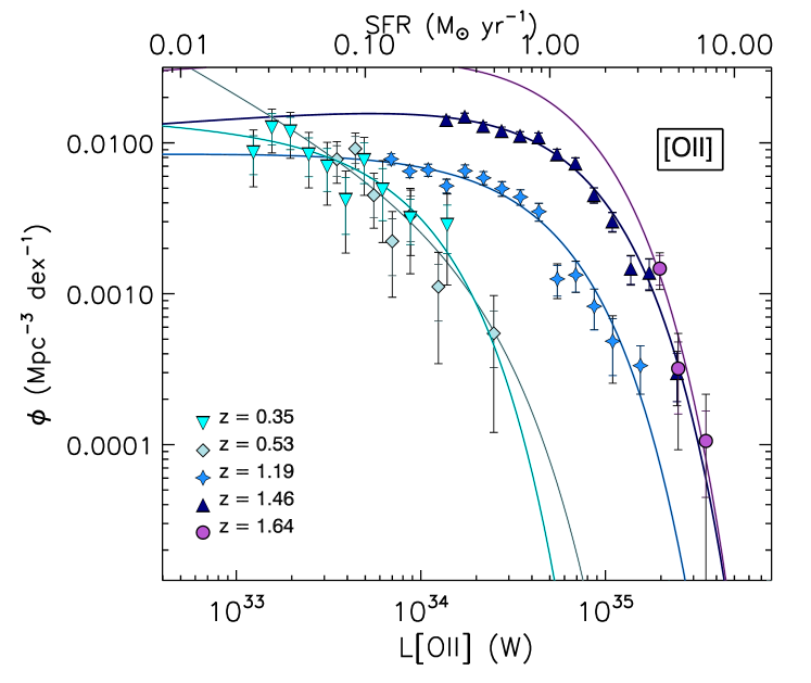
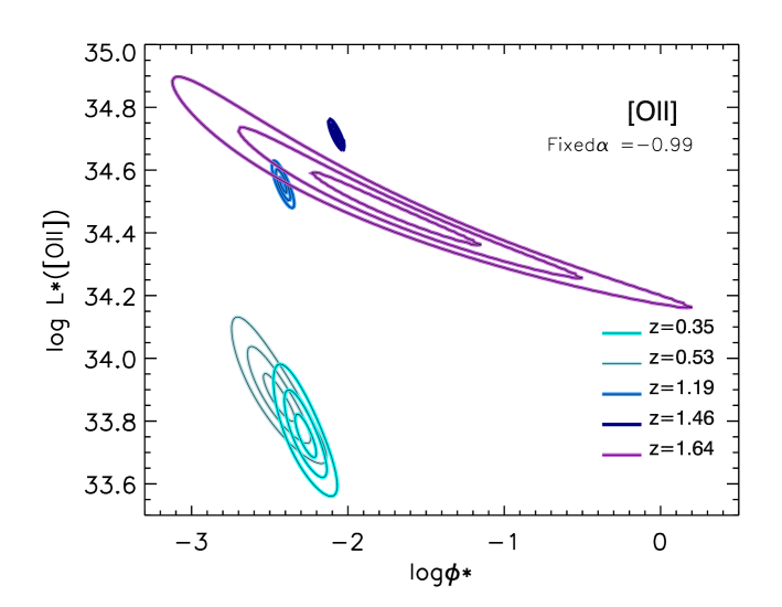
The derived luminosity functions are presented in Table 4 and Figure 9. Volumes quoted are representative of the volume covered where filter transmission is greater than 0.5. Observed (aperture-corrected) values are presented, followed by the extinction-corrected value of $L^{*}$, assuming 1 magnitude of extinction at H$\alpha$ (Kennicutt 1992; 1998) and as applied in Fujita et al. (2003), Pascual et al. (2005), Sobral et al. (2012) and Sobral et al. (2013). Figure 9 presents the best fitting LFs for the data at each redshift with the maximum likelihood fit shown in bold coloured lines. Symbols represent the binned luminosity function in bins of $\sim$0.1 dex.

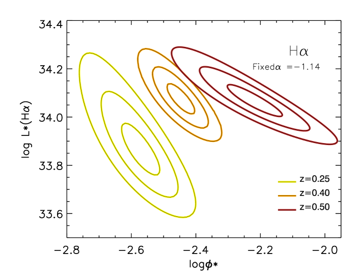
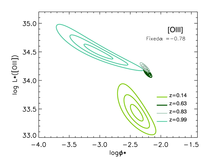
Alongside each panel of LFs, we include a graphic representation of the error ellipses of the 1, 2 and 3$\sigma$ contours in $L^{*}$-$\phi^{*}$ space representing the boundaries of the volume in 2D ($\phi^{*}$, $L^{*}$) space. We anchor $\alpha$ to the median value across the redshift slices for each line as shown in each Figure, while $L^{*}$ and $\phi^{*}$ are allowed to vary (i.e. $\alpha$ is constant per panel to allow comparison of LFs).

6.1.1 Treatment of Shallow Data

As discussed in Section 5, the maximum likelihood analysis minimizes Equation 8 allowing $\phi^{*}$, $L^{*}$ and $\alpha$ to vary. However, this analysis requires a deep and plentiful data set in order to produce a well constrained fit, particularly for $\alpha$. NB570 is the shallowest of the Subaru NB images, and due to its blue wavelength samples [O iii] emitters at a very low redshift (in the smallest cosmic volume of the analysis); consequently the LFs produced from the NB570 filter selection ([O iii] at z=0.14 and [O ii] at 0.53) are subject to low number statistics, with only 42 and 83 objects respectively making up each LF.

Furthermore, VISTA data are $\sim$1 mag shallower than NB570, and so our data struggles to probe $L^{*}$ in the $z=0.5,1.0$ and $1.6$ redshift slices, in addition to very low numbers of emitters being detected.

The shallower depth of this data means that $\alpha$ is not as well constrained as for the deeper more detection-rich LFs, however, the NB985 combined data set is selected close in wavelength to the NB921 filter, and consequently probes redshift slices only marginally more distant than the NB921 selection. To combat the shallow data we fit LFs for the 3 VISTA redshift slices with $\alpha$ constrained by a Gaussian prior based on the value for the NB921 selection for the same emission line. This is a valid method of evaluation where we do indeed have some prior knowledge of the value of $\alpha$. We take a similar approach with the NB570 [O ii] LF at $z=0.53$, setting the prior according to the [O ii] LF at $z=0.35$.

6.1.2 The Effect of Cosmic Variance

In order to study the effect of our limited number of detections we undertake a jackknife analysis in every redshift slice. For each slice we use random sampling with replacement to construct 1000 synthetic catalogues of narrow-band emitters such that each sample is of the same size as our true catalogues. We fit luminosity functions to each of these synthetic catalogues and measure the standard deviation in each parameter. These $1\sigma$ deviations are comparable to but no bigger than the uncertainties in the true dataset. Errors quoted in Table 4 refer only to the $1\sigma$ uncertainty in the real data. In Figure 9 we plot two error bars for each point. The smaller of the two error bars represents the Poissonian error, and the larger includes the standard deviation on the number of objects in each luminosity bin from the jackknifed samples added in quadrature.

Table 4: Luminosity functions in 12 redshift slices for H$\alpha$, [O iii] or [O ii] emission. Numbers of objects quoted refer to the final number of objects per luminosity function (after culling to the broadest 3$\sigma$ colour-scatter limit of the SXDS fields, and taking into account the completeness correction). Volumes refer to the volume enclosed where the filter transmission is greater than 50 per cent. Schechter fits to the data are presented with the value of L^∗ corrected for aperture effects and Galactic extinction at the wavelength of the filter. The extinction corrected values listed are those derived for 1 mag of extinction at H$\alpha$. Where the raw data did not produce a converging LF, values are absent for SFR^∗ and $\rho_{\rm{SFR}}$ as these would be non-physical.

						Extinction - corrected
Redshift	Objects	Volume	log $\phi^{*}_{\rm{H}_{\alpha}}$	log L${}^{*}_{\rm{H}_{\alpha}}$	$\alpha_{\rm{H}_{\alpha}}$	log L${}^{*}_{\rm{H}_{\alpha}}$	SFR∗	$\rho_{\rm{SFR}_{\rm{H}_{\alpha}}}$
		(104 Mpc3)	(Mpc-3)	(Watts)		(Watts)	(M⊙ yr-1)	(M⊙ yr-1 Mpc-3)
0.25	142	1.22	-2.43${}^{+0.17}_{-0.21}$	33.83${}^{+0.19}_{-0.16}$	-1.03${}^{+0.17}_{-0.15}$	34.23${}^{+0.19}_{-0.16}$	1.33${}^{+0.78}_{-0.41}$	0.0051${}^{+0.0146}_{-0.0008}$
0.4	271	2.95	-2.44${}^{+0.14}_{-0.17}$	34.16${}^{+0.13}_{-0.11}$	-1.14${}^{+0.14}_{-0.13}$	34.55${}^{+0.13}_{-0.11}$	2.85${}^{+0.99}_{-0.64}$	0.0113${}^{+0.0005}_{-0.0005}$
0.5	151	4.76	-3.27${}^{+0.55}_{-0.94}$	34.69${}^{+0.46}_{-0.27}$	-2.16${}^{+0.33}_{-0.31}$	—	—	—
0.5†	151	4.76	-2.23${}^{+0.10}_{-0.12}$	34.34${}^{+0.09}_{-0.07}$	-1.23${}^{+0.12}_{-0.13}$	34.74${}^{+0.09}_{-0.07}$	4.33${}^{+1.00}_{-0.73}$	0.0308${}^{+0.0032}_{-0.0022}$
Redshift	Objects	Volume	log $\phi^{*}_{\rm[OIII]}$	log L${}^{*}_{\rm[OIII]}$	$\alpha_{\rm[OIII]}$	log L${}^{*}_{\rm[OIII]}$	SFR∗	$\rho_{\rm{SFR}_{\rm[OIII]}}$
		(104 Mpc3)	(Mpc-3)	(Watts)		(Watts)	(M⊙ yr-1)	(M⊙ yr-1 Mpc-3)
0.14	42	0.36	-3.67${}^{+1.11}_{-\infty}$	34.60${}^{+\infty}_{-0.96}$	-1.63${}^{+0.60}_{-0.24}$	35.14${}^{+\infty}_{-0.96}$	10.17${}^{+\infty}_{-9.05}$	0.0040${}^{+\infty}_{-0.0008}$
0.63	943	8.09	-2.57${}^{+0.11}_{-0.13}$	34.44${}^{+0.09}_{-0.08}$	-1.27${}^{+0.11}_{-0.11}$	34.99${}^{+0.09}_{-0.08}$	7.16${}^{+1.65}_{-1.20}$	0.0240${}^{+0.0038}_{-0.0025}$
0.83	910	12.35	-2.25${}^{+0.07}_{-0.09}$	34.28${}^{+0.07}_{-0.08}$	-0.76${}^{+0.22}_{-0.19}$	34.83${}^{+0.07}_{-0.08}$	4.95${}^{+0.87}_{-0.83}$	0.0252${}^{+0.0780}_{-0.0084}$
0.99	32	14.69	-14.45${}^{+\infty}_{-\infty}$	38.65${}^{+\infty}_{-\infty}$	-3.78${}^{+0.36}_{-0.40}$	—	—	—
0.99†	32	14.69	-3.00${}^{+0.23}_{-0.22}$	34.70${}^{+0.14}_{-0.12}$	-0.78${}^{+0.19}_{-0.21}$	35.25${}^{+0.14}_{-0.12}$	12.97${}^{+6.22}_{-3.57}$	0.0119${}^{+0.0035}_{-0.0024}$
Redshift	Objects	Volume	log $\phi^{*}_{\rm[OII]}$	log L${}^{*}_{\rm[OII]}$	$\alpha_{\rm[OII]}$	log L${}^{*}_{\rm[OII]}$	SFR∗	$\rho_{\rm{SFR}_{\rm[OII]}}$
		(104 Mpc3)	(Mpc-3)	(Watts)		(Watts)	(M⊙ yr-1)	(M⊙ yr-1 Mpc-3)
0.35	112	2.22	-2.31${}^{+0.19}_{-0.29}$	33.90${}^{+0.20}_{-0.16}$	-1.06${}^{+0.38}_{-0.34}$	34.65${}^{+0.20}_{-0.16}$	1.11${}^{+0.65}_{-0.34}$	0.0142${}^{+0.0010}_{-0.0007}$
0.53	83	3.95	-5.55${}^{+1.75}_{-\infty}$	35.38${}^{+\infty}_{-0.84}$	-2.70${}^{+0.36}_{-0.17}$	—	—	—
0.53†	83	3.95	-2.85${}^{+0.28}_{-0.41}$	34.13${}^{+0.22}_{-0.17}$	-1.68${}^{+0.33}_{-0.31}$	34.98${}^{+0.22}_{-0.17}$	2.34${}^{+1.54}_{-0.76}$	0.0231${}^{+0.0080}_{-0.0052}$
1.19	981	19.06	-2.41${}^{+0.07}_{-0.09}$	34.61${}^{+0.07}_{-0.06}$	-0.99${}^{+0.14}_{-0.13}$	35.37${}^{+0.06}_{-0.06}$	5.76${}^{+1.01}_{-0.74}$	0.0557${}^{+0.0025}_{-0.0019}$
1.46	2218	23.09	-2.03${}^{+0.04}_{-0.06}$	34.76${}^{+0.05}_{-0.04}$	-0.91${}^{+0.11}_{-0.11}$	35.52${}^{+0.05}_{-0.04}$	8.09${}^{+0.99}_{-0.71}$	0.1796${}^{+0.0053}_{-0.0055}$
1.64	27	28.31	-2.98${}^{+0.79}_{-\infty}$	35.27${}^{+\infty}_{-0.31}$	-3.10${}^{+1.35}_{-1.15}$	—	—	—
1.64†	27	28.31	-1.68${}^{+0.50}_{-0.43}$	34.73${}^{+0.10}_{-0.11}$	-0.91${}^{+0.11}_{-0.10}$	35.49${}^{+0.10}_{-0.11}$	7.47${}^{+1.93}_{-1.67}$	0.3711${}^{+0.5775}_{-0.1951}$
$\dagger$ A Gaussian prior on $\alpha$ is applied to these luminosity functions.

Figure 9: Graphic representation of our best–fitting luminosity functions (Gaussian prior on $\alpha$ for VISTA LFs and NB570 at $z=0.53$) and their 1, 2 and 3$\sigma$ error ellipses ($\alpha$ fixed to the median value per line for comparison) in $L^{*}$-$\phi^{*}$ space. The smaller of the two error bars on each point in the lefthand panels are Poissonian, larger error bars have the 1$\sigma$ variation as estimated by our jackknifing technique added in quadrature. H$\alpha$ (top panels) [O iii] (central panels) and [O ii] (lower panels). The upper SFR scale on these plots gives an indication of the raw SFR values for these LFs, these numbers have not been corrected for dust extinction.

6.2 Star Formation Rates

We use the best-fitting Schechter function in each of the 12 redshift slices to calculate the characteristic SFR and $\rho_{\rm{SFR}}$ across 10 Gyr of cosmic time. SFRs are calculated according to the relations of Kennicutt (1998) for H$\alpha$ (Equation 14), [O ii] (Equation 16) and using the standard line ratios: H$\alpha$/H$\beta$=2.78 and [OIII]/H$\beta$=3 (Osterbrock & Ferland, 2006) to derive Equation 15 for [O iii]. Equation 15 is in good agreement with the empirical relationship of Ly et al. (2007). This method determines extinction-corrected SFRs assuming continuous star formation, Case B recombination and a Salpeter IMF.

$${{\rm{SFR}}({\rm{M}}_{\odot}{\rm{yr}}^{-1})=7.9\times 10^{-35}{{\rm{L_{H\alpha}}}{{\rm{E}(H\alpha)}}}}$$ (14)

$${{\rm{SFR}}({\rm{M}}_{\odot}{\rm{yr}}^{-1})=7.35\times 10^{-35}{{\rm{L_{[OIII]}}}}{{\rm{E}[OIII]}}}$$ (15)

$${{\rm{SFR}}({\rm{M}}_{\odot}{\rm{yr}}^{-1})=1.39\times 10^{-34}{{\rm{L_{[OII]}}}}{{\rm{E}(H\alpha)}}}$$ (16)

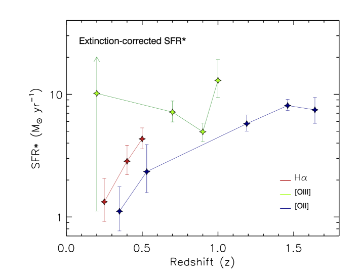
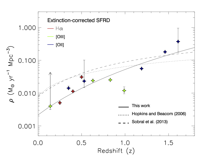
Figure 10 (a) presents the fully-corrected characteristic star formation rate (SFR*; aperture and extinction corrections described in Sections 6.1 and 5.4) for each redshift slice in this analysis, red points showing H$\alpha$ derived estimates, green, [O iii], and blue, [O ii]. Error bars represent SFRs for the corresponding 1$\sigma$ upper and lower bounds on the characteristic SFR. Figure 10(b) presents the integrated $\rho_{\rm{SFR}}$ for each LF (full integration, extinction-corrected) together with the fits of Sobral et al. (2013) and Hopkins & Beacom (2006) using the data of Baldry & Glazebrook (2003).

(a)                                                             (b)

Figure 10: Panel (a) shows the extinction-corrected characteristic star formation rate (SFR ^∗) determined in each redshift slice, error bars corresponding to the $1\sigma$ error on $L^{*}$. Colours reference the emission line used to derive the SFR. Panel (b) presents $\rho$ _SFR in each redshift slice. Colours again represent emission line used to derive the measurement. The solid black line shows our parametrization of $\rho$ ${}_{\rm{SFR}}\propto(1+z)^{4.58}$, and the dotted lines show parametrisations in the literature.

7 Discussion

7.1 Evolution of the Star Formation Rate

We find characteristic SFRs broadly consistent between all three indicators out to $z\sim 1.6$. The characteristic SFR increases by a factor $\sim 10$ between $z\sim 0.14$ and $z\sim 1.6$, in good agreement with literature results. The H$\alpha$ and [O ii] derived star formation rates show a distinct increase with redshift consistent with other studies, but we note that the [O iii] estimates (while broadly consistent with the other indicators due to their uncertainty) would produce a more convincing increase with redshift if for instance the [O iii]/H$\beta$ ratio were to decrease with redshift.

The parametrization of $\rho_{\rm{SFR}}$ according to $\rho_{\rm{SFR}}\propto$ (1+z)^γ gives $\gamma$ = 4.58 when handling errors as the maximum and minimum values of $\rho_{\rm{SFR}}$ produced from the $1\sigma$ confidence limits of each measurement of $\phi^{*}$, $L^{*}$ and $\alpha$. We note that applying the same least squares fit to the data of Ly et al. (2007) gives a slope of $\gamma$ = 4.20. Applying a blanket 10 per cent error on $\rho_{\rm{SFR}}$ to our data results in $\gamma$ = 3.02, similar to the parametrization of Sobral et al. (2013). The discrepancy between these results and shallower slopes in the literature is attributed to the small volumes probed in our low redshift slices. For instance, using the figures of Somerville et al. (2004) we expect uncertainty in $\rho_{\rm{SFR}}$ in the lowest redshift slices to be comparable to the measurements themselves due to cosmic variance. Larger areas of sky are required for this technique to be of use in determining the $\rho_{\rm{SFR}}$ at low redshift as the redshift slices sampled in narrow-band surveys are especially susceptible to cosmic variance. We return to this point in Section 7.4. We note also that the [O ii] LF of Gilbank et al. (2010) at $z\sim 1$ gives a $\rho_{\rm{SFR}}$ in good agreement with the progression of [O ii] values seen in panel 10(b).

This technique is however sensitive to particularly low SFRs, probing well below SFR^∗ ($\ll 1M_{\odot}\,{\rm{yr^{-1}}}$) in the deepest data sets allowing a more accurate evaluation of $\alpha$. While the role of these faint galaxies’ contributions to the overall $\rho_{\rm{SFR}}$ is unclear, if we wish to understand the nature of this faint population it is important to first constrain $\alpha$.

7.2 The Faint End Slope

The gradient of the faint end slope, $\alpha$, is the subject of much debate. The recent work of Sobral et al. (2013) made a significant advance on previous studies by examining estimates of $\alpha$ across a broad redshift range using the first sample of consistently selected emission line objects out to $z=2.23$. An important part of determining the most likely luminosity function at any redshift however, is to determine the significance of the galaxies we are capable of detecting in the analysis within the general population at redshift $z$. As discussed in Section 5.2, we compute the ratio of detectable galaxies to the total number of galaxies capable of hosting the line. Investigating this ratio we find that the best fit $\alpha$ of each LF is in fact very sensitive to the assumed faintest broad-band magnitude of a galaxy that can host an emission line (i.e. the denominator of this fraction). The analysis of Sobral et al. (2013) assesses emission-line detection fraction down to the limit of their NB data, and so we investigate the effect of assessing our data in the same way.

Evaluating our data set with ${m_{\rm{faint}}}$ set to the limiting NB magnitude (${m_{\rm{faint}}}$(NB)) we find that the resultant values of $\alpha$ are consistently steeper than for our ${m_{\rm{faint}}}$(EW) analysis, the medians of the two samples being offset by 0.3. Furthermore, the range in values of $\alpha$ is reduced (from $0.90$ to $0.66$) through use of the (${m_{\rm{faint}}}$(NB)) limit across the same redshift range.

Taking the well-constrained NB921 H$\alpha$ and NB921 [O ii] luminosity functions we vary the input limiting equivalent width value for ${m_{\rm{faint}}}$. The sensitivity of $\alpha$ to the input value is displayed in Figure 11. As EW${}_{m_{\rm{faint}}}$ is increased, a larger fraction of the population of galaxies can host emission lines, and so the detection fraction decreases and the resultant $\alpha$ steepens. Conversely however, as the input EW${}_{m_{\rm{faint}}}$ is lowered below 100Å the numerator of Equation 12 (the red portion of a line in Figure 8) begins to decrease when ${m_{\rm{faint}}}$ crosses the 5$\sigma$ detection limit. As the detection limit moves to brighter magnitudes, the galaxies undetected due to their position beneath the horizontal observed equivalent width limit in Figure 8 become a larger fraction of the overall population, and so the detection fraction again decreases, and $\alpha$ steepens. The shallowest $\alpha$ therefore, should correspond to the point where the NB detection limit, $m_{5\sigma}$, is equal to ${m_{\rm{faint}}}$.

Figure 11: The variation of $\alpha$ and $\rho_{\rm{SFR}}$ with differing input values of the limiting equivalent width for ${m_{\rm{faint}}}$. The upper panel shows the variation in resultant values of $\alpha$ for the NB921 [O ii] luminosity function at $z=1.46$ (blue) and the NB921 H$\alpha$ luminosity function at $z=0.40$ (red) when the limiting value of equivalent width for ${m_{\rm{faint}}}$ is varied. The lower panel shows the corresponding resultant values of $\rho_{\rm{SFR}}$ as ${m_{\rm{faint}}}$ changes for the same two luminosity functions.

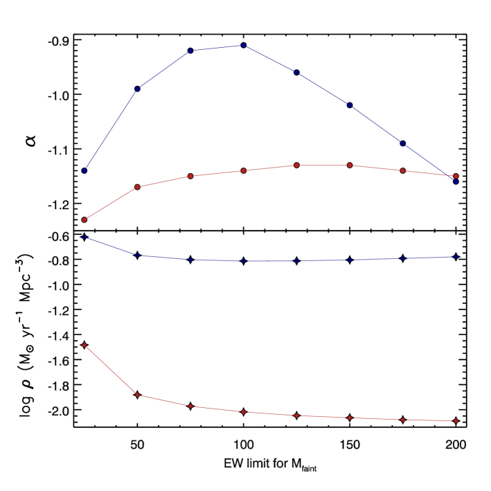
7.3 The Effect of $\alpha$ on $\rho_{\rm{SFR}}$

The effect of $\alpha$ on $\rho_{\rm{SFR}}$ is dependent on the value of $\alpha$ itself. For shallow $\alpha$, the effect is small, however, for steeper slopes the $\rho_{\rm{SFR}}$ estimate is altered more dramatically for a small change in $\alpha$. For instance, taking the well-constrained NB921 [O ii] LF at $z=1.46$ and altering $\alpha=-0.91$ by $\Delta\alpha=0.1$ in either direction (holding $\phi^{*}$, $L^{*}$ constant) causes the $\rho_{\rm{SFR}}$ to rise by $\sim 5$ per cent for steeper (more negative) $\alpha$ but only decrease by $\sim 3$ per cent for the corresponding $\Delta\alpha=0.1$ towards shallower (less negative) $\alpha$. Taking the same approach with the NB921 H$\alpha$ LF at $z=0.4$, $\alpha=-1.14$ , and the equivalent $\Delta\alpha=0.1$ changes in $\alpha$ result in a 11 per cent increase in $\rho_{\rm{SFR}}$ for steeper $\alpha$ and a 8 per cent decrease for a shallower slope. This behaviour is reflected in the lower panel of Figure 11, however it is also apparent that $\rho_{\rm{SFR}}$ increases more rapidly towards smaller limiting EW values for ${m_{\rm{faint}}}$. We interpret this as the result of an unrealistic limit to ${m_{\rm{faint}}}$ causing the detection fraction of galaxies to become very small and produce an unrealistic correction inconsistent with the data.

7.4 Comparison to Other Studies

The NB921–selected [O ii] LF and $\rho_{\rm{SFR}}$ at $z=1.46$ is in excellent agreement with the results of Sobral et al. (2012)’s UDS+Cosmic Evolution Survey (COSMOS) selection. Conversely though, comparison of our NB921-selected sample of H$\alpha$ emitters to the selection of Sobral et al. (2013) at $z=0.4$ reveals our $\rho_{\rm{SFR}}$ is much lower than the UDS+COSMOS value. However, Sobral et al. (2013) found a difference in $\rho_{\rm{SFR}}$ between their UDS and COSMOS–selected samples, with the UDS value being a factor of 3 lower than that for COSMOS. Their best-fitting LF using UDS emitters alone produces $\rho_{\rm{SFR}}=0.014\;{\rm{M_{\odot}yr^{-1}}}$ (D. Sobral, private communication) a value slightly higher than our own. We are able to fully account for this difference if we use the same method of redshift slice assignment as in Sobral et al. (2013) (where objects with K mag $>$ 23.0 were assigned according to B$-$R, i$-$K colour). Our work uses a later UDS data release and so deeper near-infrared imaging results in more accurate photometric redshifts for faint objects — these are in good agreement with Grützbauch et al. (2011). We also confirm the reliability of our aperture corrections through the agreement of $\rho_{\rm{SFR}}$ at $z=0.4$ between Sobral et al. (2013)’s UDS-only sample and our H$\alpha$ emitters according to B$-$R, i$-$K colour ($\rho_{\rm{SFR}}=0.0138\;{\rm{M_{\odot}yr^{-1}}}$). The recovery of this $\rho_{\rm{SFR}}$ despite the differing aperture sizes used for detection (Sobral et al. 2013 use a 3 arcsecond aperture at low redshift) lends support to the success of our global corrections for aperture flux loss.

As discussed in Section 6.1.2 the uncertainty in our results due to the finite number of objects detected per redshift slice is investigated via a jackknife analysis. However, it is not possible to tell if the values of $\rho_{\rm{SFR}}$ we compute are representative of the overall $\rho_{\rm{SFR}}$ at each redshift. This depends on the large scale structure in the UDS at the redshifts we sample. It is not possible to tell whether these regions are particularly under- or over-dense without a comparison to many more similar surveys. For example, in the lowest redshift slice that we sample, [O iii] at $z=0.14$, we would require a contiguous volume $\sim 140$ times larger in order for the $1\sigma$ uncertainty in number counts of galaxies to reduce to $20$ per cent according to the calculations of Somerville et al. (2004). The issue can be more efficiently addressed by observing widely separated regions of sky and comparing the variations seen to between such fields to predictions. For example the divergence of $\rho_{\rm{SFR}}$ by a factor of $\sim 3$ between this work and Sobral et al. (2012)’s UDS+COSMOS measurement at low redshift (H$\alpha$ at $z=0.40$) is quantitatively consistent with the predictions of of Somerville et al. (2004). Finally we note that our value of $\rho_{\rm{SFR}}$ at $z=1.46$ is in excellent agreement with both the $\rho_{\rm{SFR}}$ of Sobral et al. (2012)’s UDS+COSMOS measurement, and Ly et al. (2007)’s Subaru Deep Field (SDF) measurement. Based on these comparisons we note that our estimates of $\rho_{\rm{SFR}}$ in the lower redshift slices may differ from the true values by up to a factor of $\sim 8$ in the lowest redshift slice, $z=0.14$. The resultant steep value of $\gamma$ should therefore not be a cause for concern when the uncertainty due to cosmic variance is so large.

8 Conclusions

We have developed a robust method for evaluating luminosity functions which correctly handles the selection criteria of NB samples, negating the need for retrospective corrections to the data set. As a result, the method is suitable for highly irregular filters, and is applicable to a broad range of data sets. This is the first maximum likelihood analysis of narrow-band emitters using one of the largest NB-selected data sets to date. Our results can be broadly summarized as follows:

• We have presented maximum-likelihood luminosity functions in 12 redshift slices out to $z=1.64$, and demonstrated that this technique produces results in concordance with literature luminosity functions using similar data sets over similar redshift ranges. In particular we confirm the results of Sobral et al. (2013) and Sobral et al. (2012) in the $z=0.4$ and $z=1.46$ redshift slices for the H$\alpha$ and [O ii] NB921 samples respectively.

• We find the evolution of the $\rho_{\rm{SFR}}$ to rise according to $\rho_{\rm{SFR}}$ $\propto$ (1+z)^4.58 but conclude that this is strongly affected by cosmic variance in the small volumes probed at low redshift through this technique.

• While the areal coverage of this survey is not large enough to place constraints on $\rho_{\rm{SFR}}$ at low redshift, the sensitivity to very low SFRs that deep narrow-band observations provide makes this technique ideal for constraining the faint end slope.

• We discover that the detection fraction of emission lines plays an important role in the determination of the faint end slope. We propose that the limit of integration for the total number of galaxies capable of hosting an emission line should be empirically motivated, and here we base this on the line of interest’s maximum observed equivalent width in the local Universe.

• The deep NB data will still provide useful information on the population of objects making up the faint end slope, and allow an evaluation of SFR with stellar mass. We will present this analysis in a future paper.

References

- Ajiki et al. (2003) Ajiki M. et al., 2003, AJ, 126, 2091
- Arnouts et al. (2005) Arnouts S. et al., 2005, ApJ, 619, L43
- Baldry & Glazebrook (2003) Baldry I. K., Glazebrook K., 2003, ApJ, 593, 258
- Baldry et al. (2005) Baldry I. K. et al., 2005, MNRAS, 358, 441
- Bertin & Arnouts (1996) Bertin E., Arnouts S., 1996, A&AS, 117, 393
- Bouwens et al. (2010) Bouwens R. J. et al., 2010, ApJ, 709, L133
- Brammer et al. (2008) Brammer G. B., van Dokkum P. G., Coppi P., 2008, ApJ, 686, 1503
- Bunker et al. (2004) Bunker A. J., Stanway E. R., Ellis R. S., McMahon R. G., 2004, MNRAS, 355, 374
- Bunker et al. (1995) Bunker A. J., Warren S. J., Hewett P. C., Clements D. L., 1995, MNRAS, 273, 513
- Cardelli et al. (1989) Cardelli J. A., Clayton G. C., Mathis J. S., 1989, ApJ, 345, 245
- Cowie et al. (1999) Cowie L. L., Songaila A., Barger A. J., 1999, AJ, 118, 603
- Daddi et al. (2004) Daddi E., Cimatti A., Renzini A., Fontana A., Mignoli M., Pozzetti L., Tozzi P., Zamorani G., 2004, ApJ, 617, 746
- Dalton et al. (2006) Dalton G. B. et al., 2006, in Society of Photo-Optical Instrumentation Engineers (SPIE) Conference Series, Vol. 6269, Society of Photo-Optical Instrumentation Engineers (SPIE) Conference Series
- Drozdovsky et al. (2005) Drozdovsky I., Yan L., Chen H.-W., Stern D., Kennicutt, Jr. R., Spinrad H., Dawson S., 2005, AJ, 130, 1324
- Foucaud et al. (2007) Foucaud S. et al., 2007, MNRAS, 376, L20
- Fujita et al. (2003) Fujita S. S. et al., 2003, ApJ, 586, L115
- Furusawa et al. (2008) Furusawa H. et al., 2008, ApJS, 176, 1
- Gallego et al. (1995) Gallego J., Zamorano J., Aragon-Salamanca A., Rego M., 1995, ApJ, 455, L1
- Geach et al. (2008) Geach J. E., Smail I., Best P. N., Kurk J., Casali M., Ivison R. J., Coppin K., 2008, MNRAS, 388, 1473
- Gilbank et al. (2010) Gilbank D. G. et al., 2010, MNRAS, 405, 2419
- Grützbauch et al. (2011) Grützbauch R., Chuter R. W., Conselice C. J., Bauer A. E., Bluck A. F. L., Buitrago F., Mortlock A., 2011, MNRAS, 412, 2361
- Hayes et al. (2010) Hayes M., Schaerer D., Östlin G., 2010, A&A, 509, L5
- Hicks et al. (2002) Hicks E. K. S., Malkan M. A., Teplitz H. I., McCarthy P. J., Yan L., 2002, ApJ, 581, 205
- Hogg et al. (1998) Hogg D. W., Cohen J. G., Blandford R., Pahre M. A., 1998, ApJ, 504, 622
- Hopkins & Beacom (2006) Hopkins A. M., Beacom J. F., 2006, ApJ, 651, 142
- Jarvis et al. (2013) Jarvis M. J. et al., 2013, MNRAS, 428, 1281
- Kennicutt (1992) Kennicutt, Jr. R. C., 1992, ApJ, 388, 310
- Kennicutt (1998) Kennicutt, Jr. R. C., 1998, ARA&A, 36, 189
- Kodama et al. (2004) Kodama T., Balogh M. L., Smail I., Bower R. G., Nakata F., 2004, MNRAS, 354, 1103
- Lamareille (2010) Lamareille F., 2010, A&A, 509, A53
- Lawrence et al. (2007) Lawrence A. et al., 2007, MNRAS, 379, 1599
- Le Floc’h et al. (2005) Le Floc’h E. et al., 2005, ApJ, 632, 169
- Lilly et al. (1996) Lilly S. J., Le Fevre O., Hammer F., Crampton D., 1996, ApJ, 460, L1
- Ly et al. (2012) Ly C., Malkan M. A., Kashikawa N., Hayashi M., Nagao T., Shimasaku K., Ota K., Ross N. R., 2012, ApJ, 757, 63
- Ly et al. (2007) Ly C. et al., 2007, ApJ, 657, 738
- Marshall et al. (1983) Marshall H. L., Tananbaum H., Avni Y., Zamorani G., 1983, ApJ, 269, 35
- Mauch & Sadler (2007) Mauch T., Sadler E. M., 2007, MNRAS, 375, 931
- Noeske (2008) Noeske K. G., 2008, in Astronomical Society of the Pacific Conference Series, Vol. 381, Infrared Diagnostics of Galaxy Evolution, Chary R.-R., Teplitz H. I., Sheth K., eds., p. 485
- Osterbrock & Ferland (2006) Osterbrock D. E., Ferland G. J., 2006, Astrophysics of gaseous nebulae and active galactic nuclei
- Ouchi et al. (2009) Ouchi M. et al., 2009, ApJ, 706, 1136
- Ouchi et al. (2008) Ouchi M. et al., 2008, ApJS, 176, 301
- Ouchi et al. (2004) Ouchi M. et al., 2004, ApJ, 611, 660
- Pascual et al. (2005) Pascual S., Villar V., Gallego J., Zamorano J., Pelló R., Díaz C., Aragón-Salamanca A., 2005, in Revista Mexicana de Astronomia y Astrofisica Conference Series, Vol. 24, Revista Mexicana de Astronomia y Astrofisica Conference Series, Hidalgo-Gámez A. M., González J. J., Rodríguez Espinosa J. M., Torres-Peimbert S., eds., pp. 268–269
- Pérez-González et al. (2005) Pérez-González P. G. et al., 2005, ApJ, 630, 82
- Prescott et al. (2009) Prescott M., Baldry I. K., James P. A., 2009, MNRAS, 397, 90
- Saunders et al. (2004) Saunders W., Cannon R., Sutherland W., 2004, Anglo-Australian Observatory Epping Newsletter, 106, 16
- Schechter (1976) Schechter P., 1976, ApJ, 203, 297
- Schlegel et al. (1998) Schlegel D. J., Finkbeiner D. P., Davis M., 1998, ApJ, 500, 525
- Shioya et al. (2008) Shioya Y. et al., 2008, ApJS, 175, 128
- Simpson et al. (2012) Simpson C. et al., 2012, MNRAS, 421, 3060
- Sobral et al. (2009) Sobral D. et al., 2009, MNRAS, 398, 75
- Sobral et al. (2012) Sobral D., Best P. N., Matsuda Y., Smail I., Geach J. E., Cirasuolo M., 2012, MNRAS, 420, 1926
- Sobral et al. (2011) Sobral D., Best P. N., Smail I., Geach J. E., Cirasuolo M., Garn T., Dalton G. B., 2011, MNRAS, 411, 675
- Sobral et al. (2013) Sobral D., Smail I., Best P. N., Geach J. E., Matsuda Y., Stott J. P., Cirasuolo M., Kurk J., 2013, MNRAS, 428, 1128
- Somerville et al. (2004) Somerville R. S., Lee K., Ferguson H. C., Gardner J. P., Moustakas L. A., Giavalisco M., 2004, ApJ, 600, L171
- Tadaki et al. (2011) Tadaki K.-I., Kodama T., Koyama Y., Hayashi M., Tanaka I., Tokoku C., 2011, PASJ, 63, 437
- Teplitz et al. (2003) Teplitz H. I., Collins N. R., Gardner J. P., Hill R. S., Heap S. R., Lindler D. J., Rhodes J., Woodgate B. E., 2003, ApJS, 146, 209
- Tresse et al. (2002) Tresse L., Maddox S. J., Le Fèvre O., Cuby J.-G., 2002, MNRAS, 337, 369
- Umeda et al. (2004) Umeda K. et al., 2004, ApJ, 601, 805
- Villar et al. (2008) Villar V., Gallego J., Pérez-González P. G., Pascual S., Noeske K., Koo D. C., Barro G., Zamorano J., 2008, ApJ, 677, 169
- Wilson et al. (2002) Wilson G., Cowie L. L., Barger A. J., Burke D. J., 2002, AJ, 124, 1258
- Yan et al. (1999) Yan L., McCarthy P. J., Freudling W., Teplitz H. I., Malumuth E. M., Weymann R. J., Malkan M. A., 1999, ApJ, 519, L47