Parallel Chen-Han (PCH) Algorithm for Discrete Geodesics

Abstract

In many graphics applications, the computation of exact geodesic distance is very important. However, the high computational cost of the existing geodesic algorithms means that they are not practical for large-scale models or time-critical applications. To tackle this challenge, we propose the parallel Chen-Han (or PCH) algorithm, which extends the classic Chen-Han (CH) discrete geodesic algorithm to the parallel setting. The original CH algorithm and its variant both lack a parallel solution because the windows (a key data structure that carries the shortest distance in the wavefront propagation) are maintained in a strict order or a tightly coupled manner, which means that only one window is processed at a time. We propose dividing the CH’s sequential algorithm into four phases, window selection, window propagation, data organization, and events processing so that there is no data dependence or conflicts in each phase and the operations within each phase can be carried out in parallel. The proposed PCH algorithm is able to propagate a large number of windows simultaneously and independently. We also adopt a simple yet effective strategy to control the total number of windows. We implement the PCH algorithm on modern GPUs (such as Nvidia GTX 580) and analyze the performance in detail. The performance improvement (compared to the sequential algorithms) is highly consistent with GPU double-precision performance (GFLOPS). Extensive experiments on real-world models demonstrate an order of magnitude improvement in execution time compared to the state-of-the-art.

1 Introduction

Computing geodesics on triangle meshes, as a fundamental problem in geometric modeling, has been widely studied since the mid-1980s. Over the years, several algorithms have been proposed to compute the “single-source-all-destination” geodesic distance, such as, the MMP algorithm [Mitchell et al. 1987], the CH algorithm [Chen and Han 1990] and the improved CH (or ICH) algorithm [Xin and Wang 2009], the fast marching method [Kimmel and Sethian 1998] and the approximate MMP algorithm [Surazhsky et al. 2005]. While the state-of-the-art approaches [Surazhsky et al. 2005] [Xin and Wang 2009] work quite well for models of moderate size, their high computational cost means that they are not practical for large-scale models or time-critical applications.

In the past decade, there has been an increasing trend of performing the traditionally-CPU-handled computation on a graphics processing unit (GPU), which uses large numbers of graphics chips to parallelize the computation. However, developing parallel algorithms for discrete geodesics is technically challenging due to the lack of parallel structure; specifically, the geodesic distance is propagated from the source to all destinations in a sequential order. To date, the only parallel geodesic algorithm is that of Weber et al. DBLP:journals/tog/WeberDBBK08, who developed a raster scan-based version of the fast marching algorithm. Although Weber et al.’s method is highly efficient, it only computes the first-order approximation of geodesic and requires parameterization of the surface into a regular domain, which is usually difficult for surfaces with complicated geometry and/or topology. To our knowledge, there is no parallel algorithm with which to compute an exact geodesic on triangle meshes.

Technical challenges  The existing exact geodesic algorithms (for example, the MMP, CH and ICH algorithms) do not support parallel computing due to the lack of parallel structure. These algorithms partition each edge into a set of intervals, called windows, which are maintained in a queue and then propagated across the mesh faces. The propagation step pops a window from the queue and then computes its children windows and performs clipping or merging if necessary, which can add, modify, or remove existing windows, and the queue is updated accordingly. These algorithms generate the correct solution regardless of the order in which windows are removed from the queue; however, selecting windows in arbitrary order causes extremely slow performance.

The MMP algorithm and the ICH algorithm propagate the windows as a wavefront by ordering them in a priority queue according to their distance from the source. However, maintaining a priority queue is a sequential and global process. It is highly non-trivial to implement a parallel priority queue on GPUs. The performance of the MMP and ICH algorithms drops significantly without the priority queue.

The CH algorithm organizes the windows in a tree data structure and propagates the windows in a breadth-first-search sweep from the root to the leaves. Due to the data dependency between parents and their children nodes, only windows on the same level can be processed in parallel. To maintain this global tree data structure, a CPU/GPU synchronization must be conducted for each layer. As the depth of the tree equals the number of mesh faces, the $O(n)$ times synchronization is too expensive for large models, making parallel implementation unpractical.

Our contributions  This paper extends the classic CH algorithm for parallel computing the exact geodesic distance on triangle meshes. Our algorithm, which is called the Parallel Chen-Han (or PCH) algorithm, follows the window propagation framework, as all the exact algorithms do. Our idea is to divide CH’s sequential algorithm into several phases in such a way that there is no data dependence in each phase and the operations within each phase can be done in parallel. Our parallel algorithm design considers three key factors: (1) propagating the windows in as parallel a manner as possible; (2) controlling the total number of windows effectively; and (3) avoiding data conflicts during window propagation. The following concepts made it possible for us to address these issues.

• First, in contrast to the existing approaches, which maintain the windows in a “tightly-coupled” structure (such as the tree data structure in the CH algorithm) or a “strictly-ordered” structure (such as the priority queue in MMP/ICH algorithms), the windows in the proposed PCH algorithm are loosely organized. Consequently, our method neither sorts the windows nor traces the ancestor windows. Therefore, the windows can be propagated in a fully parallel and independent manner.

• Second, to reduce the total number of windows, the PCH algorithm adopts a $k$-selection to determine the $k$ windows nearest to the source, where the parameter $k$ is specified by the user. These windows will then be processed independently by multiple GPU threads. Together with a parallel $k$-selection and the window filtering techniques in the CH and ICH algorithms, our parallel algorithm is very effective for window propagation, as well as for controlling the total number of windows. Extensive evaluation of real-world models shows that our algorithm only has slightly more windows than the ICH algorithm, which uses a priority queue to maintain the wavefront.

• Third, during window propagation, if a window brings the vertex $v$ a shorter distance than its current distance, our method does not immediately update the geodesic distance at $v$ immediately, since other threads may also access $v$ at the same time and such an update would cause data conflicts. Instead, our method triggers an update event. Once all the selected windows have been propagated, our method processes these events and updates the corresponding data. This updating can also be done in a parallel manner.

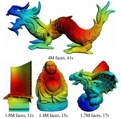
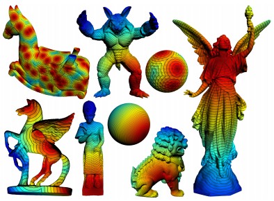
The proposed PCH algorithm is the first parallel technique for calculating exact geodesic distance on triangle meshes. We have implemented our algorithm on modern GPUs and obtained promising results on a wide range of models. We have observed that the performance improvement is highly consistent with the GPUs’ double-precision performance (GFLOPS). For example, our method can compute the exact geodesic distance field on the 1.8-million-face Blade model (see Figure 1) in 11 seconds on an Nvidia GTX580 graphics card, which is an order of magnitude faster than the state of the art [Xin and Wang 2009]. This indicates that our algorithm is suitable for applications involving intensive geodesic distance computations.

Figure 1: Computing the exact geodesic distance on triangle meshes by using the proposed PCH algorithm. Our implementation on Nvidia GTX 580 is one magnitude of order faster than [Xin and Wang 2009].

2 Related Work

The discrete geodesic problem has been widely studied since middle 80s. There are many elegant algorithms to compute the single-source-all-destination geodesic, geodesic path, geodesic loop and all-pairs geodesic. Due to the limited space, we review only the representative work of the single-source-all-destination geodesic, which is our major target.

Exact geodesic algorithms  Sharir and Schorr Sharir_Schorr:1986 pioneered the discrete geodesic algorithm with time complexity $O(n^{3}\log n)$. However, their algorithm applies only to convex polyhedral. Using a continuous Dijkstra sweep, Mitchell, Mount and Papadimitriou Mitchell_Etc:1987 presented the first practical algorithm to compute geodesic distances on general polyhedral surfaces with time complexity $O(n^{2}\log n)$. Liu et al. liu improved the robustness of the MMP algorithm by presenting effective techniques to handle the degenerate cases. Surazhsky et al. Surazhsky_Etc:2005 observed the worst case running time of the MMP algorithm is rare, and in practice the algorithm runs in sub-quadratic time. However, the MMP algorithm is memory inefficient due to its quadratic memory complexity $O(n^{2})$, which diminishes its application to large-scale models. Chen and Han Chen_Han:1990 improved the time complexity to $O(n^{2})$ by organizing the windows with a tree data structure. As only the branch nodes are saved, the CH algorithm has linear space complexity $O(n)$. Although the time complexity of the CH algorithm is better than that of the MMP algorithm, extensive experiments show that the CH algorithm runs much slower than the MMP algorithm, mainly because most of the windows in the CH algorithm are useless, which do not contribute to the shortest distance. Xin and Wang Xin_Wang:2009 presented an effective window filtering technique to reduce the windows significantly, and used a priority queue to order the windows according to the minimal distance from the source. They demonstrated that their improved CH algorithm (ICH) outperforms the MMP and CH algorithms in terms of both execution time and memory cost. Schreiber and Sharir [Schreiber and Sharir 2006] presented an $O(n\log n)$-time algorithm for convex polyhedral surfaces, which reaches the theoretical lower bound. However, the optimal time bound for general polyhedral surfaces is still an open problem. With the exact geodesic distance, Liu et al. Liu:2011:CIB:2006853.2006983 systematically investigated the analytic structure of iso-contours and bisectors on triangle meshes, and proposed efficient algorithm for computing geodesic Voronoi diagrams.

Approximation geodesic algorithms   Sethian fmm proposed the $O(n\log n)$ fast marching method for first-order approximation of geodesics on regular grids. Kimmel and Sethian Kimmel_Sethian:1998 extended the fast marching method to triangle meshes. Weber et al. DBLP:journals/tog/WeberDBBK08 presented a raster scan-based version of the fast marching algorithm for approximating the geodesic distance on geometry images. Thanks to its parallel structure, their approach allows highly efficient parallelization on modern GPUs. Polthier and Schmies Polthier_Schmies:1998 proposed the locally straightest geodesic, which differs from the conventional locally shortest geodesic. Surazhsky et al. Surazhsky_Etc:2005 presented the approximate MMP algorithm that has optimal time complexity $O(n\log n)$ and computes approximate geodesics with bounded error.

3 Preliminary

Let $M=(V,E,F)$ be a triangle mesh representing an orientable 2-manifold where $V$, $E$ and $F$ are the vertex, edge and face sets, respectively. For a vertex $v\in V$, the total angle is the sum of interior angles formed between each pair of neighboring edges incident at $v$. A vertex $v$ is called spherical if its total angle is less than $2\pi$, Euclidean if the total angle equals $2\pi$, and saddle if the total angle is greater than $2\pi$. Mitchell et al. Mitchell_Etc:1987 proved that there exists a geodesic path from the source $s$, typically a mesh vertex, to any other point on the surface. They also showed that a geodesic path cannot pass through a spherical vertex except that it is an end point.

Theorem [Mitchell et al. 1987]  The general form of a geodesic path is a path that goes through an alternating sequence of vertices and edges such that the unfolded image of the path along any edge sequence is a straight line segment and the angle of the path passing through a vertex is greater than or equal to $\pi$.

If a geodesic path from the source $s$ to destination $t$ passes through one or more saddle vertices, we call the vertex, which is nearest to $t$, a pseudo source. Clearly, a geodesic path must be a straight line inside a triangle. When crossing over an edge, the geodesic path must also correspond to a straight line if the two adjacent faces are unfolded into a common plane. The exact geodesic algorithms partition each mesh edge into a set of intervals, called windows [Surazhsky et al. 2005] [Xin and Wang 2009], each of which encodes the geodesic paths passing through the same face sequence.

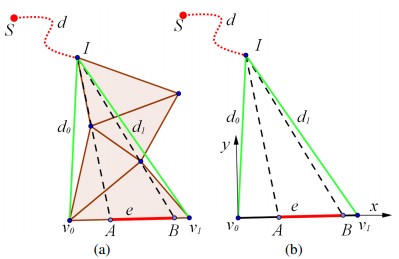
As shown in Figure 2, a window data structure associated to an edge $e$ is a $6$-tuple $(d,A,B,d_{0},d_{1},e)$ where

• $d$ is the distance from the pseudo source to the source $s$;

• $A$ and $B$ are the left and right endpoints of the interval;

• $d_{0}$ and $d_{1}$ are the distances from the edge endpoints to the (pseudo) source.

Figure 2: (a) A window represents an interval $[A,B]$ on an oriented edge $e$, which is “visible” by the pseudo source $I$ after unfolding the corresponding face sequence. (b) The position of the pseudo source on the unfolded plane can be determined by $d_{0}$ and $d_{1}$.

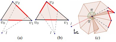
An important step in the exact geodesic algorithms is to propagate the windows across the adjacent triangle, which yields new windows on the opposite edge(s). In general, a window at edge $e$ can have up to two children at the edges opposite to $e$. See Figure 3(a)-(b). For a special case where the geodesic path passes through a saddle vertex $v$, one or more windows are then created for the edges in a fanned area. See Figure 3(c).

Figure 3: Window propagation results in new windows. (a) A window creates one child on the opposite edge. (b) A window creates two children on opposite edges. (c) For a saddle point $v$, the injection ray $l$ is split into two directions (dashed grey lines), each is an extended straight line of $l$ after unfolding. Then the new windows are generated on the opposite edges in the fanned area formed by the two directions.

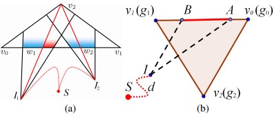
Chen and Han Chen_Han:1990 proposed using a tree data structure to keep record of the parent-child relationship. The depth of the tree is equal to the number of faces. To avoid exponential explosion in the tree, Chen and Han adopted a simple “one angle one split” scheme: if two windows occupy a vertex, at most one of them can have two children. See Figure 4(a). Xin and Wang Xin_Wang:2009 further reduced the number of windows by using a strict window filtering technique. See Figure 4(b). They also suggested using the priority queue to organize the windows according to their distance back to the source. Adopting the priority queue together with the two window filtering techniques, the ICH algorithm outperforms both the MMP and CH algorithms.

Mitchell et al. Mitchell_Etc:1987 proved that each edge may have $O(|E|)$ windows and therefore the total number of windows is $O(|E|^{2})$, which is the theoretical upper bound. In practice, Surazhsky et al. Surazhsky_Etc:2005 observed that for typical meshes an edge has an average of $O(\sqrt{|E|})$ windows. Thus, the key for developing an efficient geodesic algorithm is to organize the windows effectively.

Figure 4: Window filter. (a) The “one angle one split” filter in the CH algorithm. Two windows $w_{1}$ and $w_{2}$ share the same edge $(v_{0},v_{1})$ and occupy the vertex $v_{2}$. However, the pseudo source $I_{1}$ can not provide a shorter distance to $v_{2}$. Thus, only window $w_{2}$ can generate two children. (b) The filter used in the ICH algorithm. The window $w$ on edge $(v_{0},v_{1})$ is generated by some window on edge $(v_{1},v_{2})$. Let $g_{i}$ be the current shortest distance for vertex $v_{i}$, $i=0,1,2$. The window $w$ is useless, if one of the following inequalities holds: $d+\|IB\|>g_{0}+\|v_{0}B\|$ or $d+\|IA\|>g_{1}+\|v_{1}A\|$ or $d+\|IB\|>g_{2}+\|v_{2}B\|$.

4 Computing Geodesics in Parallel

The proposed parallel Chen-Han algorithm is based on the shared memory model so that all of the data (such as mesh data structure, geodesic distance, etc.) are assessable to all processors. This section presents our algorithm on modern GPUs, as these are readily available to the graphics community.

4.1 Data Structure

Our algorithm maintains several global variables, as shown in Table 1. Let $M=(V,E,F)$ denote the input triangle mesh, where $V$, $E$ and $F$ are the set of vertices, edges and faces. We use the half-edge data structure to encode $M$’s incidence information. Considering the limited GPU memory, we adopt a minimal half-edge data structure. Each edge is decomposed into two half-edges with opposite orientations. Each half-edge stores the index of the starting vertex, the index of the opposite half-edge and its length. Each vertex references one outgoing half-edge.

struct half_edge {
    int starting_vertex_id;
    int opposite_half_edge_id;
    double length;
};

half_edge he[]; // size 3|F|
half_edge outgoing_he[]; // size |V|

Compared to the standard half-edge data structure, our struct half_edge does not have the face that it boarders and the next half-edge around the face. The complete incidence information is encoded into two arrays, he of dimension $3|F|$, which stores all half-edges of $M$, and outgoing_he, of dimension $|V|$, which stores one of the half-edges emanating from each vertex. The three half-edges of the $i$-th triangle are stored at $he[3i]$, $he[3i+1]$ and $he[3i+2]$, respectively. Given the half_edge[$j$], the triangle that it boarders is the $\lfloor j/3\rfloor$-th triangle and the next-half-edge around that face is half_edge[$3\lfloor j/3\rfloor+(j+1)\%3$], where $\lfloor\cdot\rfloor$ is the floor function.

To access the one-ring neighbors of the $i$-th vertex $v_{i}$, one can simply start with the outgoing half-edge outgoing_he$[i]$ and iteratively switch to the opposite half-edge and find the next half-edge that points to neighboring vertex. The half-edge data structure, he and outgoing_he, are located in the GPU memory and accessible to the GPU threads in the real-only manner. The PCH algorithm does not require the vertex coordinates, instead, it needs only the metric (the edge length).

double geod_dist[]; // size |V|
window angle_split[]; // size 3|F|

The array geod_dist[0..$|V|$-1] stores the distance value at each vertex. The initial value for each non-source vertex is $\infty$. When the algorithm terminates, the value geod_dist[i] gives the globally shortest geodesic distance at the $i$-th vertex.

The array angle_split[0..3$|F|$-1] contains the window that can provide the shortest distance to each angle. Such information is used by the Chen-Han’s “one angle one split” window filter.

During the wavefront propagation, a large number of windows will be created, processed, and then discarded. To allow efficient access of the windows, our program creates a memory pool in the GPU memory. The memory pool contains all the active windows, which are stored continuously so that there are no memory gaps between adjacent windows. This condition allows us to distribute the active windows evenly to all GPU threads. The memory pool also provides each GPU thread with a buffer for the temporary storage of the new windows. The global array buffer_address[0..$T$-1] stores the beginning address and size of each buffer. Unlike the continuous storage of the active windows, these thread buffers are not physically continuous in the memory pool.

Data	Location	CPU access	GPU access
half_edge	GPU RAM	-	read only
data structure
angle_split[]	CPU RAM (mapped	read	read only
geod_dist[]	to GPU RAM)	& write
memory pool	GPU RAM	-	read & write

Table 1: Global variables.

4.2 PCH Algorithm

Let $S=\{s_{i}\}_{i=1}^{m}$ be the set of source points specified by the user. For each source point $s_{i}$, our algorithm creates a window for every edge facing $s_{i}$, and then iteratively processes the windows.

Each iteration contains the following four steps: First, the algorithm selects $k$ windows that are nearest to the source points $s_{i}$, $i=1,\cdots,m$. Second, the selected $k$ windows are processed by $T$ threads in a completely independent manner. The window propagation results in new windows, which are stored in each thread’s own buffer. If a window $w$ can provide a shorter distance for a vertex $v$, our algorithm does not immediately update the corresponding entries of $geod\_dist$ or $angle\_split$, as doing so would cause conflicts. Instead, the algorithm creates an update event, which will be processed later. Third, the algorithm collects the new windows and organizes them with the existing windows in the memory pool, so that there are no memory gaps between the adjacent windows. Finally, the algorithm processes these update events and updates the arrays $geod\_dist$ and $angle\_split$ for the corresponding vertices and corner angles.

These four steps are repeated until all windows in the memory pool have been processed. The data flow for each iteration is shown in Figure 5 and the pseudo code is shown in Algorithm 1. Next, we explain the algorithm in details.

Figure 5: During each iteration, our algorithm selects $k$ windows that are nearest to the source points and assigns these windows to $T$ GPU threads. Each window is taken by one GPU thread and then propagates independently, which will result in one or more children windows. After all the selected windows have been processed, our algorithm collects the newly-generated windows and organize all windows such that there are no memory gaps between adjacent windows in the memory pool. The empty slots in the memory pool are drawn in light gray.

1:A triangle mesh $M=(V,E,F)$, the set of source points $S=\{s_{i}|s_{i}\in V,1\leq i\leq m\}$, the selection parameter $k$, and the number of GPU threads $T$

2:The geodesic distance for each vertex

3:initialize the global variables

4:parallel create a window for every edge opposite to the source points

5:Repeat

6:     parallel select $k$ nearest windows

7:     parallel propagate the selected windows

8:     organize the newly-generated windows and update events

9:     parallel process the update events

10:Until all windows are processed

Algorithm 1 Parallel Chen-Han Algorithm

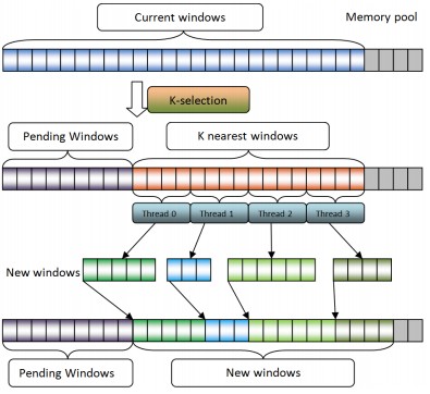
Initialization (lines 1, 2)  In the initialization stage, our algorithm creates a memory pool, and two global arrays: the first array $geod\_dist[|V|]$ contains the geodesic distance at each vertex, where the initial value is $0$ for the source points and $\infty$ for all other vertices; the second array $angle\_split[3|F|]$ contains the windows for each angle, which is used by the “one angle one split” window filter. For every edge opposite to the source point $s_{i}$, a window is created and put in the memory pool.

Step 1. Parallel selection (line 3)  Rather than sorting all windows, our algorithm selects $k$ windows, which are closest to the source points. The $k$-selection is a fundamental problem in computer science, which has been widely studied. The state-of-the art parallel algorithm is due to Monroe et al. Monroe2011. Their algorithm proceeds via an iterative probabilistic guess-and-check process on pivots for a three-way partition. When the guess is correct, the problem is reduced to selection on a much smaller set. They proved that their probabilistic algorithm always gives a correct result and always terminates. We adopt Monroe et al.’s parallel algorithm in our GPU implementation. We also develop an approximate $k$-selection to improve the speed. We choose $k\gg T$ to fully utilize the pipeline of the GPU cores. The details of optimal parameter selection and the approximated version of $k$-selection will be presented in Sec. 5.2.

Step 2. Parallel window propagation (line 4)  All of the selected windows are evenly distributed to the $T$ GPU threads. Some windows may generate one or more children, while others may not. Statistics on a wide range of real-world models show that each window generates an average maximum of $3.8$ children. Therefore, we allocate each GPU thread a $4\lceil\frac{k}{T}\rceil$-sized buffer in the memory pool to contain the new windows. This fixed-size buffer works well in practice and we do not observe any buffer overflow in our experiments. In case of an overflow in the buffer of the $i$-th thread, for example, the thread $i$ creates a new buffer of doubled size, copies the contents to the new buffer, and then updates the entry buffer_address[i]. These buffers are not required to be consecutive in the memory, since they store the new windows temporarily.

// assume $w=(d,A,B,d_{0},d_{1},e)$ is on the oriented

// edge $e=(v_{0},v_{1})$ and $v_{2}$ is the opposite vertex of $e$;

if $A=v_{0}$ && $d_{0}+d<geod\_dist[v_{0}]$ then

       // $w$ provides a short distance to $v_{0}$;

       create a distance update event $(v_{0},d_{0}+d)$;

       if $v_{0}$ is a saddle vertex then

             create windows in the fanned area (see Fig. 3(c));

      

if $B=v_{1}$ && $d_{1}+d<geod\_dist[v_{1}]$ then

       // $w$ provides a short distance to $v_{1}$;

       create a distance update event $(v_{1},d_{1}+d)$;

       if $v_{1}$ is a saddle vertex then

             create windows in the fanned area (see Fig. 3(c));

      

if $w$ occupies $v_{2}$ then

       // apply the one-angle-one-split filter;

       if $w$ provides $v_{2}$ a shorter distance than $angle\_split[v_{2}]$ then

             create an angle update event $(e,w)$;

             create $w$’s two children (see Fig. 3(b));

      else

             // $w$ has only one child on edge $(v_{0},v_{2})$ or $(v_{1},v_{2})$;

             create $w$’s child (see Fig. 4(a));

      if $\|Iv_{2}\|+d<geod\_dist[v_{2}]$ then

             create a distance update event $(v_{2},\|Iv_{2}\|+d)$;

             if $v_{2}$ is a saddle vertex then

                   create windows in the fanned area (see Fig. 3(c));

            

      

else

       // $w$ has only one child on edge $(v_{0},v_{2})$ or $(v_{1},v_{2})$;

       create $w$’s child (see Fig. 3(a));

apply the ICH filter for the new windows and store the useful

windows in the buffer (see Fig. 4(b));

Algorithm 2 PropagatingWindow($w$)

Note that during the window propagation, if a new window can provide the vertex $v$ a shorter distance than its current one $geod\_dist[v]$, we should update $geod\_dist[v]$ accordingly. However, this would cause data conflicts, as other GPU threads may also access $v$ at the same time. To avoid conflicts, we create a distance update event for $v$. Similarly, if a window $w$ occupies the vertex $v$ and provides $v$ a shorter distance than that of the window in the corresponding entry of $angle\_split$, we also create an angle update event. All these events will be processed later. The pseudo code for window propagation is shown in function PropagatingWindow().

Step 3. Data organization (line 5)  In the above window propagation step, each GPU thread $T_{i}$ generates a certain number of windows, which are stored in $T_{i}$’s own buffer. The purpose of this step is to organize these newly-generated windows in the memory pool such that there are no memory gaps between adjacent windows, which is a critical condition for the parallel selection and parallel updating.

Since each GPU thread counts the number of new windows independently, we use $O(T)$ space to store these numbers, where $T$ is the number of GPU threads. We then compute the accumulated number of new windows for each thread. Finally, each GPU thread copies its new windows from its buffer to the memory pool. The pseudo code for data organization is shown in function OrganizingData(). We use the same procedure to organize the generated distance and angle update events.

// $data_{i}$: the buffer storing the output of the $i$-th thread;

// $dataCount_{i}$: the size of $data_{i}$;

// $addr$: the address of the first free slot in the memory pool;

$cum_{0}\leftarrow 0$ ;

for $i=1$ to $T-1$ do

       $cum_{i}\leftarrow cum_{i-1}+dataCount_{i-1}$

parallel for each thread $i$ do

       copy $data_{i}$ to $addr+cum_{i}$

Algorithm 3 ReorganizeData($\{dataCount\}$, $\{data\}$, $addr$)

Step 4. Processing the update events (line 6)  The window propagating step produces distance and angle update events, which are organized in step 3 such that they are stored in the memory pool in a seamless manner. This allows us to parallel process these events.

An event is a 2-tuple $(key,value)$. For the distance update event, $key$ is the vertex id, and $value$ is the geodesic distance. For the angle update event, $key$ is id of the oriented edge, which determines the opposite angle/vertex, say $v$, and $value$ is a window occupies $v$.

To avoid the conflicts in events updating, we must sort all events by their keys in increasing or decreasing order. If two keys tie, we compare the two events by their values. For example, for two distance events $(v_{i},d^{\prime})$ and $(v_{i},d^{\prime\prime})$ occurring at the same vertex $v_{i}$, the one with smaller distance wins. To break a tie between two windows, we compare the shortest distance from the source to the corresponding interval. This tie-breaking enables us to process only the first event at a vertex or angle, since all the subsequent events occurring at the same vertex or angle do not carry useful information. We then assign the ordered events evenly to $T$ GPU threads, which update the corresponding vertices or angles. The pseudo code is shown in function ProcessingEvents().

// $event_{i}$: a 2-tuple $\{key,value\}$;

// $\{Data\}$: the to-be-updated array $geod\_dist$ or $angle\_split$;

thrust sort $\{event\}$ by $key$ and use $value$ for tie breaking;

$S\leftarrow$ size of $\{event\}$;

parallel for each thread $i$ do

       for $j=i\times\lceil\frac{S}{T}\rceil$ to $(i+1)\times\lceil\frac{S}{T}\rceil-1$ do

             if $event_{j}.key\neq event_{j-1}.key$ then

                   $Data[event_{j}.key]\leftarrow event_{j}.value$;

            

      

Algorithm 4 ProcessingEvents($\{event\}$, $\{Data\}$)

4.3 Correctness

The correctness of our parallel algorithm is based on two observations. First, during the window propagation, we adopt Chen and Han’s “one angle one split” and Xin and Wang’s filtering techniques to reduce the total number of windows. It is shown [Chen and Han 1990][Xin and Wang 2009] that both techniques remove only the useless windows, which do not carry the shortest distance. Second, Mitchell et al. Mitchell_Etc:1987 proved that there exists a geodesic path from the source $s$ to any other vertex. Our window propagation step keeps the useful windows, which carry the shortest distance. Thus, for a vertex $v$, we can always find a sequence of windows $w_{1}$, $w_{2}$, $\cdots$, $w_{l}$, to encode the geodesic path, where $w_{l}$ is the last window on the edge $e$ opposite to $v$ such that $w_{l}$ occupies the vertex $v$. So $w_{l}$ finally assigns the geodesic distance at $v$. Regardless of the order in which the windows are processed, such window sequence always exists. Thus, the resulting distance field is correct.

5 Implementation & Experimental Results

5.1 Implementation Details

We implemented our parallel geodesic algorithm on a 64-bit PC with an Intel Xeon 2.66GHz CPU and 12GB memory. The graphics card is an Nvidia GTX 580 with 512 cores and 1.5GB memory. Our program is compiled using CUDA 4.2.

The input mesh is maintained by using the half-edge data structure. Only one copy of the mesh structure is transferred to GPU memory. More specifically, we need only an array of half-edges, each of which has the length information. We do not need to store the vertex in the GPU memory; the face connectivity is also encoded in the half-edge structure.

Our algorithm requires a parallel selection to choose the $k$ nearest windows and a parallel sorting to order all update events by their keys and values. Selection and sorting can be fully implemented in parallel. We adopted the probabilistic parallel selection [Monroe et al. 2011] and CUDA’s thrust sorting [Bell and Hoberock 2011] in our implementation, but, surprisingly, observed poor performance. As shown in Figure 6 (a), the GPU selection and sorting are very slow for the 144K-face Bunny, taking more than 80% of the execution time. This slowness is mainly because the GPU selection algorithms require a large amount of CPU/GPU synchronization. As a result, these algorithms obtain good performance only for a very large number of elements (for example, more than 1 million). To improve the performance, we adopted the following simple yet effective strategies in our implementation.

Figure 6: The window selection and event sorting on the GPU take 3 to 6 seconds on the 144$K$-face Bunny model. We implement an approximate selection on the GPU and process the events on the CPU, which can significantly reduce the overall execution time. The vertical axes are the execution time in seconds and the total number of windows. The horizontal axes are the selection parameter $k$. Although the window selection is approximate, the computed geodesic distance is exact.

First, we implement an approximate $k$-selection on the GPU. Assume that there are $N(>k)$ windows, $w_{1},\cdots,w_{N}$, in the memory pool and that there are $T$ threads available. We allocate the following windows $w_{i}$, $w_{i+T}$, $w_{i+2T}$, $\cdots$, to the $i$-th thread, which enables each thread to obtain approximately $\lceil N/T\rceil$ windows, among which the $\lceil k/T\rceil$ nearest windows are selected. Thus, $T$ threads select $k$ windows in total. This approximate selection uses only a single GPU launch and can significantly reduce the execution time.

Second, since GPU sorting is not efficient, we copy the update events from GPU to CPU. To minimize the CPU/GPU data transfer, we use cudaHostAlloc() to allocate the memory for global variables $geod\_dist[]$ and $angle\_split[]$. The memory is mapped to CUDA address space using cudaHostAllocMapped, so both CPU and GPU can access it. All writing operations on such global variables are performed by CPU and the GPU procedure PropagatingWindow() accesses these data in a read-only manner. Although this CPU operation makes the event updating step sequential, we find it is much more efficient than the GPU sorting and updating and improves the overall performance significantly. See Figure 6(b).

Remark 1. Our PCH algorithm requires the windows to be stored continuously in the physical memory. This condition plays an important role in the parallel selection step, where the $i$-th thread checks the $i$, $i+T$, $i+2T$, $\cdots$, positions in the memory pool, and then selects the window nearest to the source. The continuously stored windows guarantee that each thread requires approximately the same number of windows, which means that the workload is balanced. Also, because different threads may generate different numbers of windows during the window propagation step, the procedure ReorganizeData() is required in order to reorganize the new windows and ensure the condition for the next-round parallel selection.

Remark 2. Although our implementation adopts the approximation k-selection to choose the windows, the correctness of the computed geodesic distance is guaranteed, since our algorithm does not delete any useful windows and the correctness of the geodesic distance is independent of the order in which the windows are processed. Therefore, the resulting geodesic distance is exact.

Remark 3. One of the key factors in designing a parallel algorithm is to effectively avoid data conflicts. Because our PCH algorithm propagates the windows and then updates the arrays geod_dist and angle_split in parallel, it is critical to maintain the data consistency in these arrays. Mutex and atomic operations are two commonly used techniques to access the shared memory in parallel computing. However, these techniques are not suitable to the proposed PCH algorithm, which requires frequent access of the global arrays geod_dist and angle_split: each call of PropagatingWindow reads geod_dist three times and angle_dist once. It may also write geod_dist up to three times and angle_dist once.

The large size of both arrays makes it expensive to set a mutex lock for each element. More importantly, by using mutex lock, each read/write operation locks the corresponding resources to avoid the access by other threads, which will significantly compromise the performance. On the other hand, using the atomic operations in PCH is not effective either, since doing so when reading/writing the two global arrays will slow down the procedure PropagatingWindow - the most expensive of the four steps - thereby compromising the performance of the entire program.

Therefore, our implementation does not contain the mutex or atomic operations. Instead, we adopt the delayed update strategy to avoid data conflicts. Note that the procedure PropagatingWindow does not update geod_dist and angle_dist. Thanks to the read-only operations in PropagatingWindow, all the selected $k$ windows can be propagated without any data dependence. Then, in the ProcessingEvents procedure, we sort the distance and angle updating events to detect and delete the conflicted data, after which the arrays can be updated in parallel. This delayed update strategy works quite well in practice, which is justified by the promising experimental results.

Figure 7: Testing the selection parameter $k$ on an Nvidia GTX 580 with 512 cores. The total number of windows (in red) is approximately linear proportional to the selection parameter $k$ (the horizontal axis). Choosing a small $k$ does not utilize the GPU’s parallel structure at all. On the other hand, choosing a very large $k$ would produce too many useless windows, resulting in slow performance (see the blue timing curves). We found the optimal range for $k$ is $[16\times 2^{10},24\times 2^{10}]$, which leads to the least execution time.

5.2 Parameter Setting

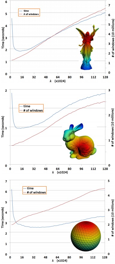
The performance of our PCH algorithm depends on the mesh complexity $n=|V|$, the GPU’s computational power (such as the number of cores and frequency), and the selection parameter $k$, which specifies the number of nearest windows to be processed by GPU threads in parallel.

The value of $k$ is closely related to the total number of windows produced in the wavefront sweep. Both the MMP algorithm and the ICH algorithm use a priority queue to determine which window is nearest to the source. Xin and Wang Xin_Wang:2009 showed that the priority queue is very effective in terms of controlling the total number of windows. If $k=1$, the $k$-selection becomes a priority queue, leading to a small number of windows. For such a case, however, our program becomes a sequential program, as only one window is processed at a time. In order to take full advantage of the parallel nature of our algorithm, a large $k$ is usually preferred, so that multiple windows can be processed independently. On the other hand, for a sufficiently large $k$, the total number of windows increases dramatically. For example, if $k$ is larger than the total number of windows, then all windows are selected and processed simultaneously, which means that the from-near-to-far wavefront is not maintained at all. As observed in both the MMP and CH algorithms, such cases will result in an extremely large number of windows and, therefore, very poor performance. Consequently, there is a trade-off between controlling the total number of windows and utilizing the GPU’s parallel structure. We tested various $k$ on a large number of models and observed that the total number of windows is almost linear to the parameter $k$; the smaller the $k$, the fewer windows, and vice versa. Figure 7 shows that the performance curves for Lucy, Bunny and Golf Ball, and the other models have very similar patterns. We found the optimal range for $k$ is $[16\times 2^{10},24\times 2^{10}]$, which leads to the least execution time.

We also investigated the relationship between the optimal range of $k$ and the mesh resolution. As Figure 8 shows, all the performance curves have the similar pattern, which reveals the trade-off between utilizing the GPU’s parallel structure and obtaining the optimal performance on the Bunny model of various resolutions. We found the optimal range of $k$ is insensitive to the mesh resolution.

Figure 8: Given the Bunny model of various resolutions, we found the optimal range of $k$ is insensitive to the mesh resolution.

Figure 9: More results.

Figure 10: The performance improvement $T_{ICH}/T_{PCH}$ is consistent with the GPU double precision performance (GFLOPS).

5.3 Performance

We tested our program on a wide range of 3D models, from the small Bunny (144K faces) to the large-scale Dragon (4 million faces). We observed that the execution time of the MMP/ICH algorithms and ours depends on the location of the source point, and that different source points may result in up to $10\%-15\%$ time difference because the total number of windows is dependent of the source point. To obtain a consistent evaluation, we repeated our test 100 times, where a random source point is generated each time. Table 3 shows the mesh complexity and the average execution time, memory cost, the number of windows, etc. The consistent experimental results show that our method obtains an order-of-magnitude improvement for models with more than 500K faces. Our algorithm is also flexible in terms of computing the “multiple-source-all-destination” geodesic distance. Table 2 shows the performance of our algorithm and the ICH algorithm on the Golf Ball and Pegasus.

# source	Golf ball			Pegasus
points	$T_{ICH}$	$T_{PCH}$	$T_{ICH}/T_{PCH}$	$T_{ICH}$	$T_{PCH}$	$T_{ICH}/T_{PCH}$
$1$	$23.71$	$2.51$	$9.45$	$32.61$	$3.33$	$9.79$
$2$	$22.02$	$2.30$	$9.59$	$33.10$	$3.04$	$10.80$
$4$	$19.36$	$2.01$	$9.65$	$29.94$	$2.83$	$10.56$
$8$	$14.61$	$1.46$	$10.04$	$34.55$	$3.16$	$10.94$
$16$	$11.17$	$1.02$	$10.90$	$31.67$	$3.40$	$9.33$
$32$	$8.49$	$0.69$	$12.32$	$26.02$	$2.83$	$9.21$
$64$	$5.99$	$0.50$	$11.97$	$24.33$	$2.34$	$10.41$
$128$	$4.60$	$0.37$	$12.53$	$20.08$	$1.99$	$10.10$
$256$	$3.62$	$0.29$	$12.65$	$15.39$	$1.57$	$9.81$
$512$	$2.85$	$0.23$	$12.46$	$12.68$	$1.25$	$10.17$
$1,024$	$2.36$	$0.20$	$12.06$	$9.95$	$0.98$	$10.15$

Table 2: Statistics of “multiple-source-all-destination” distance. Execution time was measured in seconds.

		MMP		ICH			PCH				Speedup
		Time	Peak	Time	Peak	Total	Time	Peak	Total	Peak	$T_{ICH}/T_{PCH}$
Models	# faces	(s)	mem. (MB)	(s)	mem. (MB)	#windows	(s)	mem. (MB)	# windows	# windows	Worst	Average
Bunny	$144,036$	$8.19$	$250.49$	$6.24$	$7.04$	$6,910,123$	$0.95$	$15.10$	$8,912,758$	$47,729$	$5.28$	$6.57$
Golf ball	$245,760$	$26.86$	$676.32$	$26.10$	$12.61$	$27,770,244$	$2.49$	$22.50$	$28,541,081$	$59,218$	$9.78$	$10.48$
Lion	$305,608$	$17.18$	$476.36$	$12.60$	$14.43$	$13,986,984$	$1.51$	$26.80$	$16,315,130$	$54,916$	$7.45$	$8.34$
Sphere	$327,680$	$86.94$	$1,894.02$	$70.39$	$21.55$	$81,022,375$	$8.11$	$37.08$	$82,412,805$	$201,499$	$8.51$	$8.68$
Armadillo	$345,944$	$13.25$	$412.36$	$10.34$	$15.91$	$11,169,475$	$1.40$	$28.51$	$13,159,141$	$35,599$	$6.04$	$7.39$
Lucy	$525,814$	$22.27$	$627.03$	$18.20$	$22.17$	$21,590,268$	$1.71$	$42.93$	$22,996,519$	$57,691$	$7.43$	$10.64$
Pegasus	$667,474$	$49.80$	$1,224.35$	$33.69$	$27.47$	$28,471,897$	$3.09$	$53.15$	$31,632,899$	$56,460$	$8.55$	$10.90$
Buddha	$1,439,116$	$179.67$	$3,698.71$	$160.70$	$67.42$	$113,292,750$	$15.20$	$114.77$	$122,402,062$	$139,761$	$7.95$	$10.57$
Ramesses	$1,652,528$	$76.43$	$1,734.26$	$52.09$	$57.90$	$47,374,020$	$5.79$	$124.72$	$53,404,855$	$55,083$	$7.25$	$8.99$
Gargoyle	$1,726,398$	$211.25$	$4,096.23$	$179.90$	$71.30$	$119,568,420$	$17.50$	$139.77$	$137,773,318$	$208,614$	$8.47$	$10.28$
Blade	$1,765,388$	$205.91$	$3,725.16$	$122.80$	$72.12$	$90,044,841$	$11.00$	$137.67$	$97,250,102$	$134,014$	$8.82$	$11.16$
Isidore horse	$2,208,936$	$80.85$	$2,026.17$	$67.77$	$69.04$	$56,403,922$	$6.31$	$165.04$	$68,469,783$	$54,294$	$8.95$	$10.74$
Dragon	$4,000,000$	$534.53$	$8,311.39$	$421.20$	$174.37$	$265,327,798$	$41.32$	$308.40$	$325,421,513$	$240,455$	$8.63$	$10.19$

Table 3: Model complexity and performance. Tests were repeated 100 times with random source point and the mean values are reported in this table. The last column shows both the worst and average speedup.

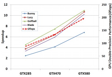
Figure 6(b) shows that GPU processing takes more than $75\%$ of the total execution time, while the corresponding ratio for large-scale models may exceed $90\%$. As all windows are processed completely in GPU, the performance of our program depends heavily on the GPU’s parallel computing capacity. We verified this by testing our program on three Nvidia graphics card: GTX 285, GTX 470 and GTX 580. As Figure 10 shows, we observed that the performance improvement $T_{ICH}/T_{PCH}$ is highly consistent with GPU double-precision performance (GFLOPS). Accordingly, we believe that our algorithm can achieve better performance on the next-generation graphics card.

In addition to performance, we also measured the peak memory of the MMP, ICH, and PCH algorithms. In order to avoid tiny windows, we adopt the same tolerance $10^{-6}$ for all the three algorithms. As Table 3 shows, the memory cost of our algorithm is much smaller than the MMP algorithm, which has $O(n^{2})$ space complexity. Our memory cost is $1.5-2$ times higher than the ICH algorithm due to the greater number of windows generated, as well as the fact that some extra space is required to store the distance and angle update events.

6 Comparison & Discussion

This section compares our method to the other exact geodesic algorithms, including the MMP algorithm, the CH algorithm, and the ICH algorithm. As mentioned before, all these algorithms do not have parallel structure.

Comparison to the MMP algorithm  The MMP algorithm takes a continuous Dijkstra sweep and maintains the windows on the wavefront using a priority queue. It is highly non-trivial to maintain the priority queue in parallel. The MMP algorithm requires windows clipping during the window propagation. The strong dependency among the windows makes it difficult to process the windows in parallel. The MMP algorithm has $O(n^{2})$ space complexity, which diminishes its application on the GPU because the GPU usually has much less RAM than CPU. Unlike the MMP algorithm, our method does not require the priority queue and window clipping operation. Our algorithm also has linear memory complexity.

Comparison to the CH algorithm  Instead of using a priority queue, the CH algorithm organizes the windows in a tree structure and propagates windows from the root to the leaves. Because only the branch nodes are retained, the CH algorithm has linear memory complexity $O(n)$. Chen and Han also proposed a “one angle one split” scheme to avoid exponential explosion. Whenever a new window $w$ occupies the vertex $v$ and provides $v$ a shorter distance, the original sub-tree at $v$ is deleted. Due to the parent-child data dependency, only windows on the same level can be processed in parallel. As a result, a CPU/GPU synchronization must be conducted for each layer. Note that the depth of the tree is equal to the number of mesh faces. Such $O(n)$ synchronization is very time consuming, which means it is not practical to parallelize the CH algorithm.

Our algorithm also adopts the “one angle one split” scheme to identify the useless windows, which do not carry the shortest distance. However, our algorithm neither has the tree structure nor maintains the parent/child relation. This allows the windows to be propagated in a fully independent manner.

Comparison to the ICH algorithm  The ICH algorithm is a variant of the CH algorithm, which adopts an effective window filtering technique to reduce the number of windows. Like the original CH algorithm, the ICH algorithm maintains the parent-child relation and the tree structure. Unlike the original algorithm, however, the window in our algorithm does not contain its parent information and no windows are sorted. This feature allows us to propagate a large number of windows in a completely independent manner.

The ICH algorithm also uses the priority queue to maintain the wavefront, which is able to minimize the total number of windows. Instead of the priority queue, our algorithm uses a simple $k$-selection to determine the windows, which are close to the source points. This strategy is very effective in terms of controlling the total number of windows. Our experimental results show that the total number of windows in our parallel algorithm is only slightly higher than that of the ICH algorithm.

The PCH algorithm on the CPU  We also implement our PCH algorithm on the CPU in such a way that all the parallel procedures are replaced by their sequential counterparts. We adopt quickselection for the sequential $k$-selection, which selects the top $k$ windows without ordering them, and then compare its performance to the ICH algorithm on the same hardware setting. We observe that the CPU PCH algorithm is 5-30% slower than the ICH algorithm for all test models.

The priority queue is known to play a critical role in the ICH algorithm, since it guarantees that the to-be-processed window is the closest to the source among all active windows. Strictly ordering the windows by their distances to the source is a very effective way to control the total number of windows. The CPU PCH algorithm selects the top $k$ windows and then propagate them one by one. Because the selected $k$ windows are not ordered, the children windows of a far-but-early-processed window may be over-ridden by a close-but-late-processed window. This means that the CPU PCH algorithm must process process 10-40% more windows than the ICH algorithm, resulting in slower performance.

The GPU PCH algorithm processes the same number of windows as the CPU PCH algorithm. However, the overhead cost of processing the extra windows is very small compared to the performance speedup by the high throughput of the GPU. Therefore, the GPU PCH algorithm significantly outperforms its CPU counterpart and the ICH algorithm.

Window deletion & complexity analysis The CH algorithm organizes the windows in a tree data structure. Chen and Han Chen_Han:1990 suggested that once a window becomes useless, the useless window and its sub-tree should be deleted (or tagged) immediately, which can guarantee the total number of windows is $O(n^{2})$, leading to an $O(n^{2})$ time complexity. Our PCH algorithm does not require the tree data structure to maintain the parent-children relation among windows. Also, it does not delete the useless windows until the update process. These features significantly reduce the data dependence, thereby providing great flexibility in the parallel algorithm design. However, the price to of such flexibility is the lack of rigorous complexity analysis.

Because time complexity is linearly proportional to the total number of windows, we empirically evaluated the time complexity by counting the total number of windows. As Table 3 shows, we observed that the total number of windows of the PCH algorithm is only 5%-20% more than that of the ICH algorithm. This implies that such a delay in windows deletion only has a very minor effect on the time complexity. As Table 3 shows, our PCH algorithm can achieve 8x-10x speedup for most of the models, which justifies the good performance of our algorithm.

7 Conclusion & Future Work

It is highly desirable to develop a parallel algorithm to compute exact geodesic on triangle meshes. However, the existing exact geodesic algorithms have very strong data dependence and lack the parallel solution. This paper presents the PCH algorithm, which extends the classic Chen-Han algorithm to parallel setting. Our idea is to divide the sequential CH algorithm into four phases, namely window selection, window propagation, data re-organization and events processing, such that the operations in each phase have no dependence or conflicts and can be done in parallel. In contrast to the original CH algorithm, the proposed PCH algorithm neither maintains the windows in a tightly coupled manner nor sorts the windows according to their distance to the source. As a result, it can process a large number of windows simultaneously and independently. We also adopt a simple selection strategy which is effective to control the total number of windows. We implemented our parallel geodesic algorithm on modern GPUs (e.g., Nvidia GTX 580) and observed that the performance improvement (compared to the conventional sequential algorithms) is highly consistent with GPU double precision performance (GFLOPS), which justifies the parallel nature of our algorithm. Extensive experiments on real-world models demonstrate an order of magnitude improvement in execution time compared to the state-of-the-art.

There are a few interesting future directions. First, we will study effective windows filtering techniques to further reduce the total number of windows, thus, improving the overall performance. Second, our PCH algorithm naturally supports the multiple-source-all-destination geodesic distance, thus, it has the potential to improve the performance of the geodesic Voronoi diagram [Liu et al. 2011]. Third, as the first parallel geodesic algorithm with good performance, the PCH algorithm is highly desired in many time-critical applications which require extensive computation of geodesics. We will investigate such applications in the near future.

References

- [\citenameBell and Hoberock 2011] Bell, N., and Hoberock, J. 2011. GPU Computing Gems, jade ed. Morgan Kaufmann Publishers, ch. Thrust: a productivity-oriented library for CUDA, 359–371.
- [\citenameChen and Han 1990] Chen, J., and Han, Y. 1990. Shortest paths on a polyhedron. In Proceedings of Symposium on Computational Geometry, 360–369.
- [\citenameKimmel and Sethian 1998] Kimmel, R., and Sethian, J. A. 1998. Computing geodesic paths on manifolds. In Proc. Natl. Acad. Sci., 8431–8435.
- [\citenameLiu et al. 2007] Liu, Y.-J., Zhou, Q.-Y., and Hu, S.-M. 2007. Handling degenerate cases in exact geodesic computation on triangle meshes. The Visual Computer 23, 9-11, 661–668.
- [\citenameLiu et al. 2011] Liu, Y.-J., Chen, Z., and Tang, K. 2011. Construction of iso-contours, bisectors, and Voronoi diagrams on triangulated surfaces. IEEE Trans. Pattern Anal. Mach. Intell. 33, 8, 1502–1517.
- [\citenameMitchell et al. 1987] Mitchell, J. S. B., Mount, D. M., and Papadimitriou, C. H. 1987. The discrete geodesic problem. SIAM J. Comput. 16, 4, 647–668.
- [\citenameMonroe et al. 2011] Monroe, L., Wendelberger, J., and Michalak, S. 2011. Randomized selection on the GPU. In Proceedings of Symposium on High Performance Graphics, 89–98.
- [\citenamePolthier and Schmies 1998] Polthier, K., and Schmies, M. 1998. Mathematical Visualization, ch. Straightest Geodesics on Polyhedral Surfaces, 391.
- [\citenameSchreiber and Sharir 2006] Schreiber, Y., and Sharir, M. 2006. An optimal-time algorithm for shortest paths on a convex polytope in three dimensions. In Proceedings of Symposium on Computational Geometry, 30–39.
- [\citenameSethian 1996] Sethian, J. 1996. A fast marching level set method for monotonically advancing fronts. Proc. Nat. Acad. Sci 93, 4, 1591–1595.
- [\citenameSharir and Schorr 1986] Sharir, M., and Schorr, A. 1986. On shortest paths in polyhedral spaces. SIAM J. Comput. 15, 1, 193–215.
- [\citenameSurazhsky et al. 2005] Surazhsky, V., Surazhsky, T., Kirsanov, D., Gortler, S. J., and Hoppe, H. 2005. Fast exact and approximate geodesics on meshes. ACM Trans. Graph. 24, 3, 553–560.
- [\citenameWeber et al. 2008] Weber, O., Devir, Y. S., Bronstein, A. M., Bronstein, M. M., and Kimmel, R. 2008. Parallel algorithms for approximation of distance maps on parametric surfaces. ACM Trans. Graph. 27, 4.
- [\citenameXin and Wang 2009] Xin, S.-Q., and Wang, G.-J. 2009. Improving Chen and Han’s algorithm on the discrete geodesic problem. ACM Trans. Graph. 28, 4, 104:1–104:8.