Fractional Standard Map: Riemann-Liouville vs. Caputo

Abstract

Properties of the phase space of the standard maps with memory obtained from the differential equations with the Riemann-Liouville and Caputo derivatives are considered. Properties of the attractors which these fractional dynamical systems demonstrate are different from properties of the regular and chaotic attractors of systems without memory: they exist in the asymptotic sense, different types of trajectories may lead to the same attracting points, trajectories may intersect, and chaotic attractors may overlap. Two maps have significant differences in the types of attractors they demonstrate and convergence of trajectories to the attracting points and trajectories. Still existence of the the most remarkable new type of attractors, “cascade of bifurcation type trajectories”, is a common feature of both maps.

1 Introduction

It is commonly accepted that fractional differential equations (FDE) play an important role in the explanation of many physical phenomena. The physical systems that can be described by FDEs, physical fractional dynamical systems (FDS), include Hamiltonian systems [1]; systems of oscillators with long range interaction [2, 3]; dielectric [4] and viscoelastic [5] materials; etc.

The FDSs with time fractional derivatives represent systems with memory. Properties of such systems can be significantly different from the properties of the systems without memory. As in the case of the regular dynamical systems, the standard map (SM), or rather the fractional standard map (FSM), is a good candidate to start studies of the general properties of the FDSs. The first study of the map with memory derived from a differential equation, fractional standard map, was done in [6]. References to the prior research of the one-dimensional maps with memory, which were not derived from the differential equations, can be found in this article. In [6] new types of attractors were found for the FSM derived from a differential equation with the Riemann-Liouville fractional derivative (FSMRL) and stability analysis was performed for the fixed and period two points.

In this article we present the results of the study of the FSM derived from a differential equation with the Caputo fractional derivative (FSMC) and compare them with the new and previously [6] obtained results for the FSMRL. The results are based on a large, but not exhaustive, number of simulations and the continuing investigation may reveal new properties of the FSMs.

2 Riemann-Liouville and Caputo Fractional Standard Maps

2.1 Equations and Initial Conditions

The standard map in the form

$$p_{n+1}=p_{n}-K\sin x_{n},\ \ x_{n+1}=x_{n}+p_{n+1}\ \ ({\rm mod}\ 2\pi)$$ (1)

can be derived from the differential equation

$$\ddot{x}+K\sin(x)\sum^{\infty}_{n=0}\delta\Bigl{(}\frac{t}{T}-(n+\varepsilon)\Bigr{)}=0,$$ (2)

were $\varepsilon\rightarrow 0+$.

The equations for Riemann-Liouville and Caputo FSMs were obtained in [7] and [8]. The Riemann-Liouville FSM can be derived from the differential equation with the Riemann-Liouville fractional derivative describing a kicked system

$$_{0}D^{\alpha}_{t}x+K\sin(x)\sum^{\infty}_{n=0}\delta\Bigl{(}\frac{t}{T}-(n+\varepsilon)\Bigr{)}=0,\quad(1<\alpha\leq 2)$$ (3)

were $\varepsilon\rightarrow 0+$, with the initial conditions

$$(_{0}D^{\alpha-1}_{t}x)(0+)=p_{1},\ \ (_{0}D^{\alpha-2}_{t}x)(0+)=b,$$ (4)

where

$${}_{0}D^{\alpha}_{t}x(t)=D^{n}_{t}\ {}_{0}I^{n-\alpha}_{t}x(t)=$$

$$\frac{1}{\Gamma(n-\alpha)}\frac{d^{n}}{dt^{n}}\int^{t}_{0}\frac{x(\tau)d\tau}{(t-\tau)^{\alpha-n+1}}\quad(n-1<\alpha\leq n),$$ (5)

$D^{n}_{t}=d^{n}/dt^{n}$, and ${}_{0}I^{\alpha}_{t}$ is a fractional integral.

The Caputo FSM can be derived from a similar equation with the Caputo fractional derivative

$$_{0}^{C}D^{\alpha}_{t}x+K\sin(x)\sum^{\infty}_{n=0}\delta\Bigl{(}\frac{t}{T}-(n+\varepsilon)\Bigr{)}=0,\quad(1<\alpha\leq 2)$$ (6)

were $\varepsilon\rightarrow 0+$, with the initial conditions

$$p(0)=(_{0}^{C}D^{1}_{t}x)(0)=(D^{1}_{t}x)(0)=p_{0},\ \ x(0)=x_{0},$$ (7)

where

$${}_{0}^{C}D^{\alpha}_{t}x(t)=_{0}I^{n-\alpha}_{t}\ D^{n}_{t}x(t)=$$

$$\frac{1}{\Gamma(n-\alpha)}\int^{t}_{0}\frac{D^{n}_{\tau}x(\tau)d\tau}{(t-\tau)^{\alpha-n+1}}\quad(n-1<\alpha\leq n),$$ (8)

After integration of equation (3) the FSMRL can be written in the form

$$p_{n+1}=p_{n}-K\sin x_{n},$$ (9)

$$x_{n+1}=\frac{1}{\Gamma(\alpha)}\sum_{i=0}^{n}p_{i+1}V^{1}_{\alpha}(n-i+1),\ \ \ \ ({\rm mod}\ 2\pi),$$ (10)

where

$$V^{k}_{\alpha}(m)=m^{\alpha-k}-(m-1)^{\alpha-k}$$ (11)

and momentum $p(t)$ is defined as

$$p(t)=\,_{0}D^{\alpha-1}_{t}x(t).$$ (12)

Here it is assumed that $T=1$ and $1<\alpha\leq 2$. The condition $b=0$ is required in order to have solutions bounded at $t=0$ for $\alpha<2$ [6]. In this form the FSMRL equations in the limiting case $\alpha=2$ coincide with the equations for the standard map under the condition $x_{0}=0$. For consistency and in order to compare corresponding results for all three maps (SM, FSMRL, and FSMC) all trajectories considered in this article have the initial condition $x_{0}=0$.

Integrating equation (6) with the momentum defined as $p=\dot{x}$ and assuming $T=1$ and $1<\alpha\leq 2$, one can derive the FSMC in the form

$$p_{n+1}=p_{n}-\frac{K}{\Gamma(\alpha-1)}\Bigl{[}\sum_{i=0}^{n-1}V^{2}_{\alpha}(n-i+1)\sin x_{i}+\sin x_{n}\Bigr{]},\ \ ({\rm mod}\ 2\pi),$$ (13)

$$x_{n+1}=x_{n}+p_{0}-\frac{K}{\Gamma(\alpha)}\sum_{i=0}^{n}V^{1}_{\alpha}(n-i+1)\sin x_{i},\ \ ({\rm mod}\ 2\pi),$$ (14)

It is important to note that the FSMC ((13), (14)) can be considered on a torus( $x$ and $p$ mod $2\pi$), a cylinder ($x$ mod $2\pi$), or in an unbounded phase space, whereas the FSMRL ((9), (10)) can be considered only in a cylindrical or an unbounded phase space. The FSMRL has no periodicity in $p$ and cannot be considered on a torus. This fact is related to the definition of the momentum (12) and initial conditions (4). The comparison of the phase portraits of two FSMs is still possible if we compare the values of the $x$ coordinates on the trajectories corresponding to the same values of the maps’ parameters.

2.2 Stable Fixed Point

The SM, the FSMRL, and the FSMC have the same fixed point at $(0,0)$. In the case of the SM this point is stable for $K<K_{cr}=4$. In the case of the FSMRL the following system describes the evolution of trajectories near the fixed point

$$\delta p_{n+1}=\delta p_{n}-K\delta x_{n},$$ (15)

$$\delta x_{n+1}=\frac{1}{\Gamma(\alpha)}\sum_{i=0}^{n}\delta p_{i+1}V_{\alpha}(n-i+1).$$ (16)

The system describing the evolution of trajectories near fixed point $(0,0)$ for the FSMC is

$$\delta p_{n+1}=\delta p_{n}-\frac{K}{\Gamma(\alpha-1)}\Bigl{[}\sum_{i=0}^{n-1}V^{2}_{\alpha}(n-i+1)\delta x_{i}+\delta x_{n}\Bigr{]},$$ (17)

$$\delta x_{n+1}=\delta x_{n}+\delta p_{0}-\frac{K}{\Gamma(\alpha)}\sum_{i=0}^{n}V^{1}_{\alpha}(n-i+1)\delta x_{i}.$$ (18)

Direct computations using equations (13), (14) show that the critical curve $K_{cr}(\alpha)$ (see Fig. 1a) such that fixed point $(0,0)$ is stable for $K<K_{cr}$ and unstable for $K>K_{c}$ in the case of the FSMC is the same as the critical curve obtained from the semi-analytic stability analysis of the FSMRL in [6]. This curve can be described by the equation

$$\frac{V_{\alpha l}K_{cr}}{2\Gamma(\alpha)}=1,$$ (19)

where

$$V_{\alpha l}=\sum_{i=1}^{\infty}(-1)^{i+1}V^{1}_{\alpha}(i).$$ (20)

Taking into account that the equations of the fractional maps (9), (10) and (13), (14) and the stability problems (15)-(18) for the maps contain convolutions, it is reasonable to introduce the generating functions

$$\tilde{X}(t)=\sum_{i=0}^{\infty}\delta x_{i}t^{i}\ \ {\rm and}\ \ \tilde{P}(t)=\sum_{i=0}^{\infty}\delta p_{i}t^{i}.$$ (21)

After the introduction

$$\tilde{W}^{1}_{\alpha}(t)=\frac{K}{\Gamma(\alpha)}\sum_{i=0}^{\infty}[(i+1)^{\alpha-1}-i^{\alpha-1}]t^{i},$$ (22)

$$\tilde{W}^{2}_{\alpha}(t)=\frac{K}{\Gamma(\alpha-1)}\Bigl{(}1+\sum_{i=1}^{\infty}[(i+1)^{\alpha-2}-i^{\alpha-2}]t^{i}\Bigr{)},$$ (23)

the stability analysis can be reduced to the analysis of the asymptotic behavior at $t=0$ of the derivatives of the analytic functions

$$\tilde{X}(t)=\frac{p_{0}\tilde{W}^{1}_{\alpha}(t)}{K}\frac{t}{1-t\Bigl{(}1-\tilde{W}^{1}_{\alpha}(t)\Bigr{)}}$$ (24)

$$\tilde{P}(t)=p_{0}\frac{1+\tilde{W}^{1}_{\alpha}(t)}{1-t\Bigl{(}1-\tilde{W}^{1}_{\alpha}(t)\Bigr{)}}$$ (25)

for the FSMRL and

$$\tilde{X}(t)=\frac{tp_{0}+(1-t)x_{0}}{(1-t)\Bigl{(}1-t+t\tilde{W}^{1}_{\alpha}(t)\Bigr{)}}$$ (26)

$$\tilde{P}(t)=\frac{1}{1-t}\Bigl{[}p_{0}-t\frac{tp_{0}+(1-t)x_{0}}{(1-t)\Bigl{(}1-t+t\tilde{W}^{1}_{\alpha}(t)\Bigr{)}}\tilde{W}^{2}_{\alpha}(t)\Bigr{]}$$ (27)

for the FSMC.

2.3 Phase Space for $K<K_{cr}$ and $1<\alpha<2$

In what follows, almost all results are conjectures. They were obtained by numerical simulations for some values of parameters $K$ and $\alpha$ and then verified for some additional values from the corresponding range of the parameters’ values.

For the area preserving standard map the stable fixed and periodic points are elliptic points - zero Lyapunov exponent. They are surrounded by the islands of regular motion. In the case of fractional maps the islands turn into basins of attraction associated with the points of attraction or slowly diverging attracting trajectories which evolve from the periodic points as $\alpha$ decreases from two. For $K<K_{cr}$ and $1<\alpha<2$ we found no chaotic or regular trajectories. Two initially close trajectories that start in the area between basins of attraction at first diverge, but then converge to the same or different attractors.

There are significant differences not only between properties of the regular and fractional standard maps but also between phase space structures of the FSMRL and FSMC. There is more than one way to approach an attracting fixed point of the FSMRL. In Fig. 1b there are two trajectories for the FSMRL with $K=2$ and $\alpha=1.4$. The bottom one is a fast converging trajectory that starts in the basin of attraction, in which $x_{n}\sim n^{-1-\alpha}$ and $p_{n}\sim n^{-\alpha}$ (see Fig. 1c). The upper trajectory is an example of the attracting slow converging trajectory (ASCT) introduced in [6] in which $x_{n}\sim n^{-\alpha}$ and $p_{n}\sim n^{1-\alpha}$ (see Fig. 1d). The trajectories that converge to the fixed point which start outside of the basin of attraction are ASCTs. In the case of the FSMC all trajectories converging to the fixed point have the same asymptotic behavior: $x_{n}\sim n^{1-\alpha}$ and $p_{n}\sim n^{1-\alpha}$ (see Fig. 1e).

In both the FSMRL and FSMC considered on a cylinder the stable fixed point $(0,0)$ is surrounded by a finite basin of attraction, whose width $W$ depends on the values of $K$ and $\alpha$. For example, for $K=3$ and $\alpha=1.9$ the width of the basin of attraction is $1.6<W<1.7$ for the FSMRL ([6]). For the FSMC with the same parameters the width is $1.7<W<1.8$. Simulations of thousands of trajectories with $p_{0}<1.6$ performed by the author, of which only 50 (with $1.6\leq p_{0}<1.7$) are presented in Fig. 1f, show only converging trajectories, whereas among 50 trajectories with $1.7\leq p_{0}<1.8$ in Fig 2b there are trajectories converging to the fixed point $(0,0)$ as well as some trajectories converging to the fixed points $(0,2\pi)$, $(0,-2\pi)$, and $(0,-4\pi)$.

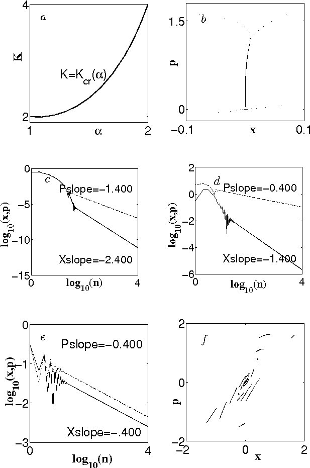
Figure 1: The FSMRL and FSMC stable fixed point $(0,0)$: a). The fixed point $(0,0)$ for both the FSMRL and FSMC is stable below the curve $K=K_{cr}(\alpha)$; b). Two trajectories for the FSMRL with $K=2$, $\alpha=1.4$, and $10^{5}$ iterations on each trajectory. The bottom one with $p_{0}=0.3$ is a fast converging trajectory. The upper trajectory with $p_{0}=5.3$ is an example of the FSMRL’s ASCT. The value of momentum on this ASCT after $10^{5}$ iterations is $p\approx 0.042$; c). Time dependence of the coordinate and momentum for the fast converging trajectory from Fig. 1b; d). $x$ and $p$ time dependence for the ASCT from the Fig. 1b; e). $x$ and $p$ time dependence for the FSMC with $K=2$, $\alpha=1.4$, and $p_{0}=0.3$; f). Evolution of the FSMC trajectories with $p_{0}=1.6+0.002i$, $0\leq i<50$ for the case $K=3$, $\alpha=1.9$. The line segments correspond to the $n$th iteration on the set of trajectories with close initial conditions. The evolution of the trajectories with smaller $p_{0}$ and for the FSMRL with the same $K$, $\alpha$, and $p_{0}<1.6$ is similar.

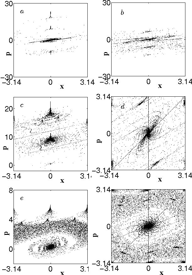
Figure 2: The FSMRL and FSMC phase space for $K<K{cr}$: a). The FSMRL with the same values of parameters as in Fig 1f but $p_{0}=1.6+0.002i$, $0\leq i<50$; b). The FSMC with the same values of parameters as in Fig 1f but $p_{0}=1.7+0.002i$, $0\leq i<50$; c). 400 iterations on the FSMRL trajectories with $p_{0}=4+0.08i$, $0\leq i<125$ for the case $K=2$, $\alpha=1.9$. Trajectories converging to the fixed point, ASDTs with $x=0$, and period 4 ASDTs are present; d). 100 iterations on the FSMC trajectories with $p_{0}=-3.14+0.0314i$, $0\leq i<200$ for the same case as in Fig. 2c ($K=2$, $\alpha=1.9$) but considered on a torus. In this case all trajectories converge to the fixed point or period four stable attracting points; e). 400 iterations on trajectories with $p_{0}=2+0.04i$, $0\leq i<50$ for the FSMRL case $K=0.6$, $\alpha=1.9$. Trajectories converging to the fixed point and ASDTs of period 2 and 3 are present; f). 100 iterations on the FSMC trajectories with $p_{0}=-3.14+0.0314i$, $0\leq i<200$ for the same case as in Fig. 2e ($K=0.6$, $\alpha=1.9$) considered on a torus. In this case all trajectories converge to the fixed point, period two and period three stable attracting points.

Another significant difference between two fractional standard maps is that all periodic points of the SM, except the fixed point $(0,0)$, in the case of the FSMRL evolve into periodic attracting slowly diverging trajectories (ASDT) (see Figs. 1a, 1c, 1e), whereas in the case of the FSMC they evolve into the corresponding attracting points (see Figs. 1b, 1d, 1f; in Figs. 1d, 1f the FSMC is considered on a torus). Presence of only period one structures in the phase spaces of two fractional standard maps in the case $K=3$, $\alpha=1.9$ (Figs. 1a, 1b) corresponds to the fact that the SM with $K=3$ has only one central island. Period $T=4$ structures in Figs. 1c, 1d and period $T=2$ and $T=3$ in Figs. 1e, 1f correspond to the phase spaces of the SM with $K=2$ and $K=0.6$. Numerical evaluation ([6]) shows that ASDTs which converge to trajectories along the $p$-axis ($x\rightarrow x_{lim}=0$) have the following asymptotic behavior: $x_{n}\sim n^{1-\alpha}$ and $p_{n}\sim n^{2-\alpha}$.

2.4 The FSMRL’s Phase Space for $K>K_{cr}$ ($1<\alpha<2$)

For $K_{cr}<K<K_{cr2}(\alpha)\leq 2\pi$, the FSMRL has period $T=2$ symmetric with respect to the origin stable points with the property

$$p_{n+1}=-p_{n},\ \ x_{n+1}=-x_{n},$$ (28)

which evolve from $T=2$ points with the same property of the SM, stable for $4<K<2\pi$. $K_{cr2}$ is the upper with respect to $K$ limit of stability of these $T=2$ points.

Assumption $(x_{n+1},p_{n+1})=(-x_{n},-p_{n})=(x_{l},p_{l})$ in system ((9), (10)) leads asymptotically ($n\rightarrow\infty$) to

$$x_{l}=\frac{K}{2\Gamma(\alpha)}V_{\alpha l}\sin(x_{l}),$$ (29)

$$p_{l}=\frac{K}{2}\sin(x_{l}),$$ (30)

which has been analyzed in [6]. The condition of solvability of (29) is

$$K>K_{cr}(\alpha)=\frac{2\Gamma(\alpha)}{V_{\alpha l}},$$ (31)

which means that the stable $T=2$ points appear when the fixed point becomes unstable.

An example with $K=4.5$ of the evolution of the FSMRL’s phase space with the decrease of $\alpha$ (from $\alpha$ on the critical curve or from 2 for $4<K<2\pi$) is presented in Fig. 3. For large values of $\alpha$ ($1.74<\alpha<2$ for $K=4.5$) the phase space has a pair of stable symmetric $T=2$ attracting points (Fig. 3a), which in the case $4<K<2\pi$ evolve from the centers of the corresponding period two islands of stability of the SM. As in the case of the fixed point, there are two types of convergence to the attracting points: slow with $\delta x_{n}\sim n^{-\alpha}$, $\delta p_{n}\sim n^{1-\alpha}$ and fast with $\delta x_{n}\sim n^{-1-\alpha}$, $\delta p_{n}\sim n^{-\alpha}$. For lower values of $\alpha$ ($1.67<\alpha<1.73$ for $K=4.5$) there appears a couple of the non-symmetric stable period two sets of attracting points (Fig. 3b), which with the decrease in $\alpha$ ($1.63<\alpha<1.66$ for $K=4.5$) transform into attracting cascade of bifurcations type trajectories (CBTT) (Figs. 3c, 3d). With the further decrease in $\alpha$ the whole phase space of the FSMRL becomes chaotic (Fig. 3e). When $\alpha$ is close to one there appears a single chaotic attractor, which at the lowest values of $\alpha$ ($\alpha<1.02$ for $K=4.5$) turns into a set of disjoint chaotic attractors (Fig. 3f).

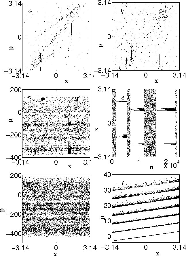
Figure 3: The FSMRL’s phase space for $K=4.5>K{cr}$: a). Period $T=2$ stable attracting points $x_{n+1}=-x_{n}$, $p_{n+1}=-p_{n}$ for $\alpha=1.8$ 500 iterations on each of 25 trajectories: $p_{0}=0.0001+0.08i$, $0\leq i<25$. Slow and fast converging trajectories. b). Two sets of $T=2$ stable attracting points $x_{n+1}\neq-x_{n}$, $p_{n+1}\neq-p_{n}$ for $\alpha=1.71$. 500 iterations on trajectories with the same initial conditions as in Fig. 3a; c). 25000 iterations on a single trajectory with $\alpha=1.65$, $p_{0}=0.3$. The trajectory occasionally sticks to one of the cascade of bifurcation type trajectories but then always recovers into the chaotic sea; d). Time dependence of the coordinate $x$ in Fig. 3c; e). 20000 iterations on a single chaotic trajectory with $\alpha=1.45$, $p_{0}=0.3$; f). 7 disjoint chaotic attractors for $\alpha=1.02$. 1000 iterations on each of 20 trajectories: $p_{0}=0.0001+1.65i$, $0\leq i<20$.

The evolution of the FSMRM’s phase space can also be considered for a fixed value of $\alpha$ (in this paragraph we consider an example with $\alpha=1.6$) and $K$ increasing from the value $K_{cr}$. When the value of $K$ is slightly above the critical curve the phase space has a pair of stable symmetric $T=2$ attracting points ($K_{cr}<K<3.9$ for $\alpha=1.6$). A couple of non-symmetric stable $T=2$ sets of attracting points appears for $4<K<4.2$; CBTTs exist for $4.3<K<4.4$; for $K>4.5$ the whole phase space seems chaotic.

It should be noted that the existence of the CBTTs can’t be attributed to the fact of the unusual definition of momentum in the derivation of the FSMRL. The values of $x$-coordinates in Fig. 3d represent the solutions of the original differential equation (3) independently of the definition of momentum.

2.5 The FSMC’s Phase Space for $K>K_{cr}$ and $1<\alpha<2$

Figure 4: The FSMC’s phase space for $K=4.5>K{cr}$: a). Period $T=2$ stable attracting points $x_{n+1}=-x_{n}$, $p_{n+1}=-p_{n}$ for $\alpha=1.8$. 1000 iterations on each of 10 trajectories: $p_{0}=-3.1415+0.628i$, $0\leq i<10$. b). Two sets of $T=2$ stable attracting points $x_{n+1}\neq-x_{n}$, $p_{n+1}\neq-p_{n}$ for $\alpha=1.71$. 1000 iterations on trajectories with the same initial conditions as in Fig. 4a; c). 30000 iterations on a single trajectory with $\alpha=1.65$, $p_{0}=0.3$. The CBTTs can hardly be recognized on the full phase portrait, but can be seen on the $x$ of $n$ dependence in Fig. 4d; d). Time dependence of the coordinate $x$ in Fig. 4c; e). 20000 iterations on a single trajectory with $\alpha=1.45$, $p_{0}=0.3$; f). 20000 iterations on each of two overlapping independent attractors for $\alpha=1.02$. The CBTT has $p_{0}=-1.8855$ and the chaotic attractor $p_{0}=-2.5135$.

Numerical simulations show that the FSMC also has the period $T=2$ symmetric stable point for $K>K_{cr}$. After $10^{5}$ iterations the difference in the values of $x_{l}$ for two maps is less than $10^{-5}$. The order of the difference in the values of $p_{l}$ is ten percent. Fig. 4 gives an example of the evolution of the FSMC’s phase space with the decrease in $\alpha$ for $K=4.5$. The intervals of the existence of the symmetric $T=2$ points, asymmetric sets of the $T=2$ points, and CBTTs are approximately the same for both maps. Trajectories converging to the symmetric $T=2$ points follow the same law as the trajectories converging to the fixed point: $\delta x_{n}\sim n^{1-\alpha}$, $\delta p_{n}\sim n^{1-\alpha}$. It is difficult to resolve the CBTTs on the phase portrait of the system (Fig. 4c) and to recognize on a zoom but they are very clear on the $x$ of $n$ dependence in Fig 4d. The values of the $x$-coordinates of the CBTTs for the FSMRL and FSMC are very close. For $\alpha<1.6$ the phase space becomes chaotic with very nonuniform density of points (Fig. 4e). With the further decrease in $\alpha$ there appear chaotic attractors and then a set of disjoint and overlapping attractors. In Fig. 4f one can see two overlapping attractors for $\alpha=1.02$. The CBTT on this picture (a dark set) persists even after 300000 iterations and overlaps with the chaotic attractor.

The observed overlapping of attractors and intersection of trajectories in phase spaces is a consequence of the fact that the considered fractional systems are systems with memory. In such systems the coordinates of the next trajectory point are functions of the coordinates of all previously visited points on a trajectory. In this case a coincidence of two points does not lead to a coincidence of trajectories, and this property is very different from the properties of phase spaces of the regular dynamical systems.

3 Conclusion

In this paper we continued the study of fractional maps started in [6]. We concentrated on the comparison of two maps at the values of the FSM parameter $K<2\pi$. Even though the simulations were not exhaustive, we were able to show that there are significant similarities as well as differences between the structures of the phase space of two FSMs. One of the findings is that the CBTTs are more common in fractional maps than we originally thought. We hope that computer simulations of the equations of the physical systems that are described by the fractional differential equations will also produce the CBTTs and their origin will have a proper physical interpretation.

References

- Zaslavsky [2005] Zaslavsky GM. Hamiltonian Chaos and Fractional Dynamics. Oxford: Oxford University Press; 2005.
- Tarasov and Zaslavsky [2006] Tarasov VE, Zaslavsky GM. Fractional dynamics of coupled oscillators with long-range interaction. Chaos 2006;16:023110.
- Zaslavsky et al. [2007] Zaslavsky MA, Edelman M, Tarasov VE. Dynamics of the chain of forced oscillators with long-range interaction: from synchronization to chaos. 2007;17:043124.
- Tarasov [2008] Tarasov VE. Universal electromagnetic waves in dielectrics. J Phys.: Condens. Matter 2008;20:175223.
- Mailnardi [2010] Mainardi F. Fractional Calculus and Waves in Linear Viscoelasticity: An Introduction to Mathematical Models. Singapore: World Scientific Publishing; 2010.
- Edelman and Tarasov [2009] Edelman M, Tarasov VE. Fractional standard map. Phys. Let. A 2009;374:279–285.
- Tarasov and Zaslavsky [2008] Tarasov VE, Zaslavsky GM. Fractional equations of kicked systems and discrete maps. J. Phys. A 2008;41:435101.
- Tarasov [2009] Tarasov VE. Differential equations with fractional derivative and universal map with memory. J. Phys. A 2009;42:465102.