The weak bound state with the non-zero charge density as the LHC 126.5 GeV state

Abstract

The self-consistent model of classical field interactions formulated as the counterpart of the quantum electroweak model leads to homogeneous boson ground state solutions in presence of non-zero extended fermionic charge density fluctuations. Two different types of electroweak configurations of fields are analyzed. The first one has non-zero electric and weak charge fluctuations. The second one is electrically uncharged but weakly charged. Both types of configurations have two physically interesting solutions which possess masses equal to 126.67 GeV at the value of the scalar fluctuation potential parameter $\lambda$ equal to $\sim 0.0652$. The spin zero electrically uncharged droplet formed as a result of the decay of the charged one is interpreted as the $\sim 126.5$ GeV state found in the Large Hadron Collider (LHC) experiment. (The other two configurations correspond to solutions with masses equal to 123.7 GeV and $\lambda$ equal to $\sim 0.0498$ and thus the algebraic mean of the masses of two central solutions, i.e., 126.67 GeV and 123.7 GeV, is equal to 125.185 GeV.) The problem of a mass of this kind of droplets will be considered on the basis of the phenomenon of the screening of the fluctuation of charges. Their masses are found in the thin wall approximation.

I Introduction

In Dziekuje_Jacek_nova_2 , the non-linear self-consistent model of classical field interactions in the “classical counterpart of the electroweak Glashow-Salam-Weinberg” (CGSW) model was proposed. Homogeneous boson ground state solutions in this model in the presence of non-zero extended fermionic charge density fluctuations were reviewed and fully reinterpreted in order to make the theory with non-zero charge densities JacekManka coherent as, unfortunately, the language in JacekManka uses both quantum field theory (QFT) concepts and the classical charge distributions. The model concerns the bound states of the matter of these fluctuations inside one droplet of fields. Because of the Pauli exclusion principle, only one or (for the sake of opposite projections stochastic_projection_Grossing ; stochastic_projection_Keppeler , Dziekuje_za_EPR-Bohm ; Dziekuje_za_skrypt of the spin) two fermionic fluctuations in one droplet can occupy at their lowest energy state. Unless other quantum numbers are assigned to these fluctuations, the consecutive fermionic fluctuations can eventually occupy their higher energy states. Concerning the phenomenon of the screening of the fluctuation of charges inside one droplet, we face the problem of the mass of this kind of droplet. The phenomenon of the gamma transparency of the electrically uncharged configuration of fields in the droplets in the reference to gamma bursts was previously pointed out in MarekJacek . Below, the Schrödinger-Barut background of the model is given.
The analyzed CGSW model is not a modification of the quantum GSW model Arbuzov-Zaitsev . For instance, the configurations of fields are not the structures of QFT; most particularly the ground state is not the QFT vacuum state. Hence, the argument against “a non-zero vacuum expectation value” is not relevant here since in the body of the self-consistent field theory, a structure like this does not exist at all. Unlike QFT, the self-consistent field theory (SCFT) deals with continuous charge densities and continuous charge density fluctuations as the basic concept Dziekuje_Jacek_nova_2 ; Dziekuje_za_self-consistent .
In order to present the idea of the ground field in a broader context, let us draw our attention to the Lagrangian density ${\cal L}$ of electromagnetism, which serves as an example for introducing the ground field notion in terms of the self-consistent theory only

$${\cal L}=\bar{\Psi}(\gamma^{\mu}i\partial_{\mu}-m)\Psi+J^{\mu}\,A_{\mu}-\frac{1}{4}\,F_{\mu\nu}\,F^{\mu\nu}\,,$$

where $J^{\mu}=-e\bar{\Psi}\gamma^{\mu}\Psi$ is the electron current density fluctuation and $A_{\mu}$ is the total electromagnetic field four-potential $A_{\mu}=A^{e}_{\mu}+A^{s}_{\mu}$, where the superscript $e$ stands for the external field and $s$ stands for the self-field adjusted by the radiative reaction to suit the electron current and its fluctuations (see Barut-1 ; Barut-2 ; Barut-3 ; Barut-4 , B-Nonlinear-1 ; B-Nonlinear-2 ). Then, in the minimum of the corresponding total Hamiltonian, the solution of the equation of motion for $A^{s}_{\mu}$ is called the electromagnetic ground field.
In this paper, the term boson ground field is used for the solution of equations of motion for a boson field in the ground state of the whole system of fields (fermion fluctuations, gauge bosons, scalar fluctuation) that are under consideration. This boson field is a self-field (or can be treated as one) when it is coupled to a source-“basic” field. In general, the term “basic” field means a wave function that is proper for a fermion (fluctuation), a scalar (fluctuation) or a dilatonic field Dziekuje_CI_PANIE_JEZU_CHRYSTE ; Dziekuje_za_neutron and, although not in this paper, a charged or heavy boson (which in this case plays simultaneously the role of both the basic and ground field).
The above mentioned concept of a wave function and the Schrödinger wave equation is dominant in the nonrelativistic physics of atoms, molecules and condensed matter Sakurai . In the relativistic quantum theory, this notion has been largely abandoned in favor of the second quantized perturbative Feynman graph approach, although the Dirac wave equation is still used for the approximation of some problems.
What Barut and others did was to extend the Schrödinger’s “charge density interpretation” of a wave function (e.g. the electron is the classical distribution of charge) to a “fully-fledged” relativistic theory. They successfully implemented this “natural (fields theory) interpretation” of a wave function with coupled Dirac and Maxwell equations (for characteristic boundary conditions) in many specific problems. But the “natural interpretation” of the wave function can be extended to the Klein-Gordon equation Dziekuje_CI_PANIE_JEZU_CHRYSTE ; Dziekuje_za_neutron coupled to the Einstein field equations, thus being a rival for quantum gravity in its second quantization form. In the case of the QFT models, the second quantization approach is connected with the probabilistic interpretation that is inherent in the quantum theory, whereas the classical field theories and the “natural interpretation” of the wave function together with the self-field concept are in tune with the deterministic interpretation forming a relativistic SCFT.
Thus, depending on the model, the role of a self-field can be played by e.g. the electromagnetic field bib_B-K-1 ; relativ_Lamb ; ion-collisions , spontaneous-1 ; spontaneous-2 , bib_B-D ; Casimir , boson $W^{+}-W^{-}$ and $Z$ ground-field (as below in this paper) Dziekuje_Jacek_nova_2 ; JacekManka or by the gravitational field (metric tensor) $g_{\mu\nu}$ Dziekuje_CI_PANIE_JEZU_CHRYSTE ; Dziekuje_za_neutron . The “basic” field that is proper for a particular matter source is the dominant factor in the existence of self-fields.
When the values of masses of fundamental fermionic, scalar and bosonic fields have to be taken as the external parameters of the model, then in SCFT the basic fields are in fact interpreted as fluctuations Jaynes-1 ; Jaynes-2 ; Jaynes-3 , Milonni (of the total basic fields) and the self-fields are coupled to the fluctuations only. The conjecture is that if all fluctuations are identical to their total basic fields, then the solution is fully self-consistent and the masses of all fields should appear in the result of the solution of the coupled partial differential equations that characterize the system Frieden-1 ; Frieden-2 ; Frieden-3 ; Frieden-4 ; Frieden-5 , Dziekuje_za_skrypt ; Dziekuje_za_models_building . In Frieden-1 ; Frieden-2 ; Frieden-3 ; Frieden-4 ; Frieden-5 it was shown that the structural information of the system Dziekuje_informacja_2 ; Dziekuje_informacja_1 ; Dziekuje_za_EPR-Bohm is, in the case of the scalar field, proportional to its squared rest mass. The (observed) structural information principle put upon the system means that the analyticity requirement of the log-likelihood function of the system Dziekuje_informacja_2 ; Dziekuje_za_EPR-Bohm is used. The coupled set of self-consistently solved partial differential equations arises when the variational information principle, which minimizes the total physical information of the system Frieden-1 ; Frieden-2 ; Frieden-3 ; Frieden-4 ; Frieden-5 , Dziekuje_informacja_2 is also put upon the system. (In the analyses, the Rao-Fisher metricity of the statistical space Amari-Nagaoka_book of the system is used Dziekuje_za_channel ; Dziekuje_za_EPR-Bohm .)
If only some of the fluctuations are identified with their total basic fields, then all masses of the fundamental fields remain among the parameters Dziekuje_za_channel that (at least at some value of the energy) are to be estimated from the experiment.
In accordance with the statement above, a model of bound states of fluctuations (index $f$) was constructed Dziekuje_Jacek_nova_2 . The new, electrically and/or weakly charged physical configuration lies in the minimum of the effective potential of the scalar field fluctuation $\varphi_{f}$ at the value $\varphi_{f}=\delta$, which is calculated self consistently from the Lagrangian of the CGSW model. In the model, the scalar field $\varphi$ exists inside the droplet of the configuration of fields only. It is the only one (inside the droplet) to which its fluctuation $\varphi_{f}\equiv\varphi$ is possibly equivalent (possibly, as this paper neither proves nor disproves it). In fact, it could be an effective one, e.g. the superposition of other fundamental fields or their fluctuations.
Thus, from now on, the symbols $\varphi_{f}$, $L_{f}$, $R_{f}$, respectively, denote the fluctuation of the scalar field and a doublet of left-handed or a singlet of right-handed fluctuations of fermionic fields, respectively, and not the global fields. In agreement with the above explanations of the self-consistent approach, fields in a doublet $L_{f}={\nu_{fL}\choose\ell_{fL}}$ and a singlet $R_{f}=(\ell_{fR})$ are wavefunctions, where $\ell_{f}$ and $\nu_{f}$ signify a leptonic fluctuation $\ell$ and a fluctuation of its neutrino $\nu$, respectively. Thus fields in $L_{f}$ and $R_{f}$ are not connected with the interpretation of the corresponding full (global) charge density distributions for particles in the doublet $L$ and singlet $R$, as it is for fields ruled by the original linear Dirac equation. Instead, they are associated with the distributions of the charge density fluctuations of fields in the doublet $L$ and singlet $R$ that are ruled by the coupled Dirac-Maxwell equations, similar to that found in Barut’s case. Therefore, $j_{f\,Y}^{\,\mu}$ and $j_{f}^{\,a\mu}$, $a=1,2,3$ are the continuous matter current electro-weak density fluctuations extended in space (and not operators of QFT with point-like charges). In order to simplify the calculations, the mass $m_{f}$ of any fermionic fluctuation is neglected (see Eq.(105)).
In Section II the effective potential for the “boson ground fields induced by matter sources” configuration (hereafter, I will call it the bgfms configuration) and the general algebraic equations that follow from the field equations of motion for the fields on the ground state inside the droplet are presented. They form the screening condition of the fluctuation of charges. Such quantities as the observed charge density fluctuations are also determined. In Section III the numerical results for the electrically and weakly charged bgfms (EWbgfms) configuration are presented along with the calculations of the mass of its droplet in the thin wall approximation. Section IV is devoted to an analysis of the weakly charged bgfms (Wbgfms) configuration and its stability for the sake of both the weak charge density fluctuation and $\lambda$ parameter (which is the parameter of the scalar fluctuation potential). In Section V the intersections of the $\lambda$-functions of the mass of the droplet for the electrically charged (i.e. EWbgfms) and electrically uncharged (i.e. Wbgfms) configurations are analyzed. Two of such pairs of bgfms configurations are found and analyzed: one with a mass equal to 123.7 GeV and the other with 126.67 GeV. Then, the Wbgfms configuration with a mass equal to 126.67 GeV is interpreted as the state found in the LHC experiment cms2 ; atlas2 (the Wbgfms configuration with a mass equal to 123.7 GeV is also considered). Also, in Section V the decay and gamma transparency of the Wbgfms configuration are described. After the Conclusions, in Appendix 1 the Table with some quantum numbers of fields in the $SU_{L}(2)\times U_{Y}(1)$ CGSW model are given. In Appendix 2 the field equations for the gauge self-fields and the scalar field fluctuation in CGSW model with continuous matter current density fluctuations are given. The calculations below are in the “natural units” $\hbar=c=1$.

II Boson ground state solutions

In the CGSW model the Lagrangian density for the fluctuations and self-fields coupled to them with the hidden $SU_{L}(2)\times U_{Y}(1)$ symmetry is as follows

$$\!\!\!\!\!\!\!\!\!\!\!\!\!\!\!{\cal L}_{f} = -\frac{1}{4}F^{a}_{\mu\nu}F^{a\mu\nu}-\frac{1}{4}B_{\mu\nu}B^{\mu\nu}+(D_{\mu}\Phi_{f})^{+}D^{\mu}\Phi_{f}$$ (1)

$$- \lambda(\Phi_{f}^{+}\Phi_{f}-\frac{v^{2}}{2})^{2}+{\cal L}_{f}^{\;f}\,,$$

where ${\cal L}_{f}^{\;f}$ is the fermionic part of the fluctuation sector

$$\!\!\!\!\!\!\!\!\!\!\!\!\!\!\!{\cal L}_{f}^{f} = i\bar{L}\gamma^{\mu}\nabla_{\mu}L_{f}+i\bar{R}_{f}\gamma^{\mu}\nabla_{\mu}R_{f}$$ (2)

$$- \sqrt{2}\,\frac{m_{f}}{v}(\bar{L}_{fL}\Phi_{f}\,R_{f}+\;h.c.)\;\;.$$

Here, $v=246.22\;{\rm GeV}$ particle_data and $\lambda\neq 0$ is the constant parameter of the scalar fluctuation potential, whose value will be established later on. To simplify the calculations, we neglect the mass $m_{\ell_{f}}$ of the fermionic fluctuation.
The fields inside the bgfms droplet are either the classical fluctuations of fields or classical self-fields and in this paper they are treated as such. Because the formalism for the self-consistent treatment of the quantum fields operators is not known, therefore the fields of the self-consistent approach are not the ones of a quantum field theory origin. The same is true for the quantum fluctuation fields operators. This concerns the scalar fluctuation doublet and all fermionic fluctuations and bosonic self-fields inside the bgfms configuration. Moreover, both the bosonic self-fields and the scalar and fermionic fluctuations that compose the bgfms configuration are not directly observed. What is observed is the droplet of the bgfms configuration. In this respect, the clarifying (only) similarity is to think of the neutron as a kind of configuration of fields. It is hard to prove that it consists of a proton and an electron (although see Santilli_1 ; Santilli_2 ). Similarly, it would be risky to call the fermionic fluctuation inside the droplet, e.g. a particular lepton fluctuation, although in the CGSW model the field fluctuations inside the droplet are granted the $SU_{L}(2)\times U_{Y}(1)$ quantum numbers (see Table in Appendix 1). For example, the electrically charged EWbgfms state found in Section V has the $SU_{L}(2)\times U_{Y}(1)$ quantum numbers of the fermionic fluctuation(s), which are the same as the numbers of the positron. Also, the scalar fluctuation potential $\lambda(\Phi_{f}^{+}\Phi_{f}-\frac{v^{2}}{2})^{2}$ in the CGSW model is the one for the classical scalar field fluctuation $\Phi_{f}$ that exists inside the bgfms configuration only and not for the Higgs field. In conclusion, the CGSW model is the one of the fluctuations of basic (scalar or fermionic) fields and the self-fields coupled to them. The scalar or fermionic fluctuations can be the objects different than the ones known from, e.g. the scattering experiments, but the self-fields $W^{\pm}$, $Z$ and $A$, although they are also not the quantum fields in the CGSW model, nevertheless they are the classical counterparts of the Standard Model (SM) bosonic fields and can be named after them.
Finally, the question remains as to what is the host object for the droplet of the bgfms configuration? Let us begin with the similarity of an electron in an atom. The self-field concept, as developed by Barut and Kraus, has been used successfully to compute nonrelativistic and relativistic Lamb shifts bib_B-K-1 ; relativ_Lamb . In their approach, the host object is the electron and the tiny Lamb shift of its wave mechanical energy state arises from the electron fluctuation coupled self consistently to its classical electromagnetic self-field. The self-consistent solution for the Lamb shift is then obtained iteratively (and because of this it is sometimes seen as inferior to the perturbative quantum electrodynamics (QED)). In this paper the situation is similar but, the energy of the host fermion (or fermions), if it was, e.g. the electron (or electronic fluctuation), appears to be minute in comparison to the obtained mass of the bgfms configuration.

In Eqs.(1)-(2) the covariant differentiations $\nabla_{\mu}$ for the scalar fluctuation doublet $\Phi_{f}$ and for a fermionic field fluctuations doublet $L_{f}$ and singlet $R_{f}$ are

$$\nabla_{\mu}\Phi_{f}=\partial_{\mu}\Phi_{f}+igW_{\mu}\Phi_{f}+\frac{1}{2}ig^{\prime}YB_{\mu}\Phi_{f}\;\;,$$ (3)

$$\nabla_{\mu}L_{f} = \partial_{\mu}L_{f}+igW_{\mu}L_{f}+\frac{1}{2}ig^{\prime}YB_{\mu}L_{f}\;,$$

$$\;\;\;\;\;\nabla_{\mu}R_{f} = \partial_{\mu}R_{f}+\frac{1}{2}ig^{\prime}YB_{\mu}R_{f}\;,$$ (4)

where

$$W_{\mu}=W_{\mu}^{a}\,\frac{\sigma^{a}}{2}$$ (5)

is the gauge field decomposition with respect to the $su(2)$ algebra generators. The $U_{Y}(1)$ self-field tensor is defined as

$$B_{\mu\nu}=\partial_{\mu}B_{\nu}-\partial_{\nu}B_{\mu}$$ (6)

and the $SU_{L}(2)$ Yang-Mills self-field tensor as

$$F_{\mu\nu}^{a}=\partial_{\mu}W_{\nu}^{a}-\partial_{\nu}W_{\mu}^{a}-g\varepsilon_{abc}W_{\mu}^{b}W^{c}_{\nu}\;,$$ (7)

where the symbol $\varepsilon_{abc}$ signifies the structure constants for $SU_{L}(2)$, which are antisymmetric with the interchange of two neighbour indices and $\varepsilon_{123}=+1$.
The fundamental constants of the model are the coupling constant for $SU_{L}(2)$, which is denoted by $g$, and the coupling constant for $U_{Y}(1)$, which according to convention is denoted by $g^{\prime}/2$. The weak hypercharge operator for the $U_{Y}(1)$ group is called $Y$. The quantum numbers in the model are given in the Table (Appendix 1).
Now, the scalar fluctuation doublet

$$\Phi_{f}=\frac{1}{\sqrt{2}}{0\choose\varphi_{f}}$$ (8)

contains the scalar field fluctuation $\varphi_{f}$. We have adopted the notation

$$L_{f}={\nu_{fL}\choose\ell_{fL}}\;\;{\rm and}\;\;R_{f}=(\ell_{fR})\;,$$ (9)

where for the sake of transparency only one leptonic fluctuation $\ell$ inside the bgfms and its neutrino fluctuation are specified. The contribution from other existing fermionic fluctuations can be treated in a similar way.

Now, for our charged (electroweak or weak) physical configuration at $\varphi_{f}=\delta$, we decompose the total self-fields $W^{a}_{\mu}$, $B_{\mu}$ and the scalar field fluctuation $\varphi_{f}$, which stay on the LHS of Eq.(13) as follows

$$\left\{\begin{array}[]{lll}W^{a}_{\mu}=\omega^{a}_{\mu}+\tilde{W}^{a}_{\mu}\;,\\ B_{\mu}=b_{\mu}+\tilde{B}_{\mu}\;,\\ \varphi_{f}=\delta+\tilde{\varphi}_{f}\;.\end{array}\right.$$ (13)

Here, each of the total fields on the RHS is decomposed into the self consistently treated part $\omega^{a}_{\mu}$, $b_{\mu}$ and $\delta$ and the wavy (non-self consistent) part $\tilde{W}^{a}_{\mu}$, $\tilde{B}_{\mu}$ of the self-fields and $\tilde{\varphi}_{f}$ of the scalar field fluctuation, respectively. The wavy terms are not treated self consistently. In this paper the thin wall approximation is used in which $\omega^{a}_{\mu}$, $b_{\mu}$ and $\delta$ are constant. These homogenous components of the self-fields are the main quantities which we are interested in and they are searched for self consistently on the ground state denoted as $\left(\;\right)_{0}$. The other, wavy parts of the self-fields do not enter into the self-consistent calculation in the presented model. Nevertheless, the wavy parts are important in determining the modified mixing angle $\Theta$ (see Eq.(49)) and in estimating the range of the validity of the thin wall approximation.

II.1 The screening condition of the fluctuation of charges

Now, the effective potential on the ground state is given by

$${\cal U}^{ef}_{f}=-\left({\cal L}_{f}\right)_{0}\;,$$ (14)

where ${\cal L}_{f}$ is the Lagrangian density (see Eq.(1)) of the CGSW model. Let $J_{fY}^{\,\mu}$ and $J_{f}^{\,a\mu}$ be the continuous matter current density fluctuations extended in space (see Eqs.(103-104)) equal on the ground state to

$$J_{fY}^{\,\mu}=\left(\overline{L_{f}}\gamma^{\mu}YL_{f}+\overline{R_{f}}\gamma^{\mu}YR_{f}\right)_{0}\;\;$$

$${\rm and}\;\;J_{f}^{\,a\mu}=\left(\overline{L_{f}}\gamma^{\mu}\frac{\sigma^{a}}{2}L_{f}\right)_{0}\;,$$ (15)

respectively.
We now assume that on the ground state, for the system in the local rest coordinate system we have

$$J_{fY}^{\,0}=\varrho_{fY}\;\;,\;\;J_{fY}^{i}=0\;\;,\;\;J_{f}^{\,a0}=\varrho_{f}^{\,a}\;\;{\rm and}\;\;J_{f}^{\,ai}=0\;,$$ (16)

where $\varrho_{fY}$ and $\varrho_{f}^{\,a}$ are the matter charge density fluctuations related to $U_{Y}(1)$ and $SU_{L}(2)$, respectively. Eq.(16) determines the ground state which is not relativistically covariant, hence locally, inside the discussed droplets of the fluctuations, the Lorentz invariance might not be its fundamental property (the symmetry of the Lagrangian density (2) still remaining). Yet, we will see that their diameter in the analyzed cases is only of the order of $0.001\;fm$ (see Sections III.2 and IV.1).
Remark: This means that although some characteristics of these objects may be detectable, the effects of the violations of the Lorentz invariance might remain undetectable or marginally detectable in the present experiments. Similar to the case of partons, which although small are observed, although not all of their characteristics are detectable. The literature on the possibility of the violation of the Lorentz invariance is notable Lorentz_Ferrero ; Lorentz_Diaz ; Lorentz_Peck .

As all of the analyses in this paper that pertain to the ground fields are performed on the ground state, therefore, if it is not necessary, the denotation $\left(\,\right)_{0}$ will be omitted.
Thus, what will be finally found is really the ground state of a system, which follows from the fact that the analyzed droplets of the fields of the excited configurations that lie near the physically interesting solutions have real non-negative squared masses of all their constituent fields. The stability of solutions for the particular configurations of fields is one of the basic problems analyzed in this paper. The particular ground state configurations can decay via radiation or the decay of the constituent fields only. There were attempts to approach to such phenomena on the basis of the self-energy rather than on the basis of the quantized radiation field Barut-Huele-1985 .
The self-fields which are calculated from (14) are the ground state fields and only these self-fields are treated fully self consistently in this model. The boson fields, $W^{a}_{\mu}$, $B_{\mu}$ and $\varphi_{f}$ (see Eq.(13)), which in the ground state of the whole configuration of fields are naturally called the ground fields, are denoted as $\omega^{a}_{\mu}$, $b_{\mu}$ and $\delta$, respectively

$$\!\!\!{\rm self\!\!-\!consistent\;(parts\;of)\;self\!\!-\!fields}\;\;\left\{\begin{array}[]{lll}W^{a}_{\mu}=\omega^{a}_{\mu}\;,\\ B_{\mu}=b_{\mu}\;,\\ \varphi_{f}=\delta\;.\end{array}\right.$$ (20)

They are searched for self consistently.
Next, we assume that also in the decomposition (13) in the excited states of the system, the self-consistent parts $\omega^{a}_{\mu}$, $b_{\mu}$ of the self-fields and $\delta$ are found from the self-consistent analysis of potential ${\cal U}^{ef}_{f}$ given by Eq.(14) and that in the excited states matter current density fluctuations are the same as $J_{fY}^{\,\mu}$ and $J_{f}^{\,a\mu}$ given by Eqs.(II.1),(16).
The self-consistent parts (both on the ground state and on the excited ones) can be parameterized in the following way JacekManka

$$\omega^{a}_{\mu}=\left\{\begin{array}[]{lll}\omega^{a}_{0}=\sigma\,n^{a}\;,\\ \omega^{a}_{i}=\vartheta\,\varepsilon_{aib}\,n^{b}\;\;\;{\rm and}\;\;\;n^{a}n^{a}=1\;,\end{array}\right.$$ (23)

$$b_{\mu}=\left\{\begin{array}[]{lll}b_{0}=\beta\;,\\ b_{i}=0\;.\end{array}\right.$$ (26)

In Eq.(23) the $(n^{a})=constant$ plays the role of a unit vector in the adjoint representation of the Lie algebra $su(2)$. It determines the direction of the ground fields (or more generally of the self-consistent part of the self-fields). It can be seen that (no summation over index “a”)

$$\!\!\!\omega^{a}_{\mu}\omega^{a\mu}=\sigma^{2}n^{a}n^{a}-\vartheta^{2}\varepsilon_{aib}\varepsilon_{aib}n^{b}n^{b}\;\;\;{\rm and}\;\;\;b_{\mu}b^{\mu}=\beta^{2}.$$ (27)

Now, further calculations are performed in the thin wall approximation in which $\omega^{a}_{\mu}$, $b_{\mu}$ and $\delta$ are the homogenous fields.
Using Eqs.(20)-(26) in Eqs.(14) and (1), we obtain the effective potential

$${\cal U}^{ef}_{f}(\vartheta,\sigma,\beta,\delta)\!\! = \!\!-g^{2}\sigma^{2}\vartheta^{2}+\frac{1}{2}g^{2}\vartheta^{4}-\frac{1}{8}g^{2}\delta^{2}(\sigma^{2}-2\vartheta^{2})$$ (28)

$$+ \frac{1}{4}gg^{\prime}\delta^{2}\beta\sigma n^{3}-\frac{1}{8}g^{\prime 2}\delta^{2}\beta^{2}+g\varrho_{f}^{\,a}n^{a}\sigma$$

$$+ \frac{g^{\prime}}{2}\varrho_{fY}\beta+\frac{1}{4}\lambda(\delta^{2}-v^{2})^{2}\;,$$

for the self-consistent parts of the self-fields. For the self-fields on the ground state, the potential ${\cal U}^{ef}_{f}(\vartheta,\sigma,\beta,\delta)$ forms the complete effective potential.
When the self-consistent parts of fields are homogenous in time and space, then $\vartheta$, $\sigma$, $\beta$ and $\delta$ are constant and from $\partial_{\nu}\vartheta=\partial_{\nu}\sigma=\partial_{\nu}\beta=\partial_{\nu}\delta=0$, $\nu=0,1,2,3$, it follows that $\nabla^{2}\vartheta=\nabla^{2}\sigma=\nabla^{2}\beta=\nabla^{2}\delta=0$. This means that (in the thin wall approximation) the self-consistent part of the self-fields and the scalar field fluctuation form an incompressible matter. Then, the field equations Eqs.(100)–(102) and Eq.(105) (see Appendix 2) that resulted from the CGSW Lagrangian (1) give the following four algebraic equations for the self-consistent parts $\vartheta$, $\sigma$, $\beta$ of the self-fields and $\delta$ of the scalar field fluctuation

$$\left[\;\;\frac{1}{2}\delta^{2}-2\sigma^{2}+2\vartheta^{2}\;\;\right]\vartheta=0\;,$$ (29)

$$-g(2\vartheta^{2}+\frac{1}{4}\delta^{2})\sigma+\frac{1}{4}g^{\prime}\delta^{2}\beta n^{3}+\varrho_{f}^{\,a}n^{a}=0\;,$$ (30)

$$\frac{1}{2}(g\sigma n^{3}-g^{\prime}\beta)\delta^{2}+\varrho_{fY}=0\;,$$ (31)

$$\Biglb[\;-\,\frac{1}{4}g^{2}(\sigma^{2}-2\vartheta^{2})+\frac{1}{2}gg^{\prime}\sigma\beta n^{3}-\frac{1}{4}g^{\prime 2}\beta^{2}$$

$$+\,\lambda\,(\delta^{2}-v^{2})\;\Bigrb]\;\delta=0\;.$$ (32)

In the self-consistent homogenous case, Eqs.(100)–(102) and Eq.(105) are equivalent to

$$\partial_{\vartheta}{\cal U}^{ef}_{f}=\partial_{\sigma}{\cal U}^{ef}_{f}=\partial_{\beta}{\cal U}^{ef}_{f}=\partial_{\delta}{\cal U}^{ef}_{f}=0\;,$$ (33)

and thus Eqs.(29)-(II.1) can be easily checked. They form the self-consistent part of the screening condition of the fluctuation of charges, which is the analog of the screening current condition in electromagnetism Aitchison-Hey-bis . They are used in the calculations of the value of change of the observed electric and weak density fluctuations of charges (see Eqs.(39)-(II.1) below) and the effective masses of the fields (see Eqs.(43)-(II.2) below). The self-fields obtained self consistently, i.e. according to Eqs.(29)-(II.1), will be called the self-consistent fields. The configuration of the self-consistent fields on the ground state is called (in agreement with the Introduction) the (boson) ground fields induced by matter sources (bgfms) configuration JacekManka . (They can be equivalently obtained self consistently from the effective potential given by Eq.(28) and Eq.(33).)

When we define the “electroweak magnetic field” as ${\cal B}^{a}_{i}=1/2\varepsilon_{ijk}F^{a}_{jk}$ and the “electroweak electric field” as ${\cal E}^{a}_{i}=F^{a}_{i0}$, then their self-consistent parts $(\sigma=constant,\vartheta=constant,\beta=constant,\;(n^{a})=constant)$ for $\vartheta\neq 0$ are equal to $\left({\cal B}^{a}_{i}\right)_{0}$ and $\left({\cal E}^{a}_{i}\right)_{0}$, respectively JacekManka

$$\!\!\!\left({\cal B}^{a}_{i}\right)_{0}=-g\vartheta^{2}n^{i}n^{a}\;\;\;{\rm and}\;\;\;\left({\cal E}^{a}_{i}\right)_{0}=g\sigma\vartheta(\delta_{ai}-n^{a}n^{i})\,.$$ (34)

Now, let us choose

$$(n^{a})=(0,0,1)\;.$$ (35)

In this case the self-consistent parts of the electroweak magnetic field $\left({\cal B}^{3}_{3}\right)_{0}=-g\vartheta^{2}$ along the $x^{3}$ spatial direction and of the electroweak electric field $\left({\cal E}^{1}_{1}\right)_{0}=\left({\cal E}^{2}_{2}\right)_{0}=g\sigma\vartheta$ pointing in the $x^{1}$ and $x^{2}$ spatial directions, respectively, are different from zero.

Let us perform (for $\delta\neq 0$), a “rotation” of $W^{3}_{\mu}$ and $B_{\mu}$ self-fields to the physical self-fields $Z_{\mu}$ and $A_{\mu}$

$${Z_{\mu}\choose A_{\mu}}={{cos\Theta\;\;{-sin\Theta}}\choose{sin\Theta\;\;\;\;\;cos\Theta}}{W^{3}_{\mu}\choose B_{\mu}}\;.$$ (36)

Then, consequently a rotation of $\sigma$ and $\beta$ self-consistent fields to their counterparts $\zeta$ and $\alpha$ (and similarly for $\tilde{Z}_{\mu}$ and $\tilde{A}_{\mu}$) as well as a rotation of the charge density fluctuations $\varrho_{f}^{\,3}$ and $\varrho_{fY}$ to their corresponding physical quantities $\varrho_{fZ}$ and $\varrho_{fQ}$ are as follows

$${\zeta\choose\alpha}={{cos\Theta\;\;{-sin\Theta}}\choose{sin\Theta\;\;\;\;\;cos\Theta}}{\sigma\choose\beta}\;,$$ (37)

$${(g/cos\Theta)\varrho_{fZ}\choose(gsin\Theta)\varrho_{fQ}}={{cos\Theta\;\;{-sin\Theta}}\choose{sin\Theta\;\;\;\;\;cos\Theta}}{(g)\varrho_{f}^{\,a}n^{a}\choose(g^{\prime}/2)\varrho_{fY}}\;.$$ (38)

It is worthwhile to write the relations between weak isotopic charge density fluctuation $\varrho_{f}^{\,3}$ (see Eq.(16) and Eq.(35)), weak hypercharge density fluctuation $\varrho_{fY},$ standard relation (SR) unscreened electric charge density fluctuation $\varrho_{fQ\;SR}$ (Eq.(II.1) below), standard (SR) unscreened weak charge density fluctuation $\varrho_{fZ\;SR}$ (Eq.(II.1) below) and their generalizations in our model, i.e. the observed electric charge density fluctuation $\varrho_{fQ}$ and the observed weak charge density fluctuation $\varrho_{fZ}$

$$\varrho_{fQ}=\varrho_{fQ\;SR}+\frac{1}{2}(\frac{g^{\prime}}{g}ctg\Theta-1)\varrho_{fY}\;,$$ (39)

$$\varrho_{fZ}=\varrho_{f}^{\,3}-\varrho_{fQ}\;sin^{2}\Theta\;,$$ (40)

$$\varrho_{fQ\;SR} = \varrho_{f}^{\,3}+\frac{1}{2}\varrho_{fY}\;\;\;$$

$${\rm and}\;\;\;\varrho_{fZ\;SR} = \varrho_{f}^{\,3}-\varrho_{Q\;SR}\;sin^{2}\Theta_{W}\;.$$ (41)

Here, $\Theta$ is the modified mixing angle (given below), whereas the Standard Model (SM) relations between the Weinberg angle $\Theta_{W}$, $g$ and $g^{\prime}$ are given by $cos\Theta_{W}=\frac{g}{\sqrt{g^{2}+g^{\prime 2}}}$ and $sin\Theta_{W}=\frac{g^{\prime}}{\sqrt{g^{2}+g^{\prime 2}}}$.

The numerical calculations are performed with the Fermi coupling constant equal to $G_{F}\approx 1.16638\times 10^{-5}\;{\rm GeV}^{-2}$, the SM value for the boson $W^{\pm}$ mass, $m_{W\,SM}\approx 80.385$ ${\rm GeV}$, and $sin^{2}\Theta_{W}\approx 0.23116$ particle_data . From these values, $g=\sqrt{8\,m_{W\,SM}^{2}\,G_{F}/\sqrt{2}\;}\approx 0.65295$ and $g^{\prime}=g\,tg\Theta_{W}\approx 0.35803$ and $v=2\,m_{W\,SM}/g$ $\approx 246.22\;{\rm GeV}$ are calculated. The accuracy of the results is restricted by the accuracy of the measurement of the boson $W^{\pm}$ mass $(80.385\pm 0.015\;{\rm GeV})$ particle_data , i.e., to the fourth significant digits.

II.2 The masses of the self-fields and scalar field fluctuation

The massive Lagrangian density for the boson self-fields and the scalar field fluctuation, which follows from the kinematical part of the Lagrangian (1) is equal to

$${\cal L}_{mass}\! = \!\!-\frac{1}{2}g^{2}\varepsilon_{abc}\varepsilon_{ade}\omega^{b}_{\mu}\omega^{d\,\mu}{\tilde{W}}^{c}_{\nu}{\tilde{W}}^{e\,\nu}+\frac{1}{8}g^{2}\delta^{2}{\tilde{W}}^{a}_{\mu}{\tilde{W}}^{a\,\mu}$$

$$- \frac{1}{4}gg^{\prime}\delta^{2}{\tilde{W}}^{3}_{\mu}{\tilde{B}}^{\mu}+\frac{1}{8}g^{\prime 2}\delta^{2}{\tilde{B}}_{\mu}{\tilde{B}}^{\mu}$$

$$+ \frac{1}{8}g^{2}\omega^{a}_{\mu}\omega^{a\,\mu}{\tilde{\varphi}}_{f}^{2}-\frac{1}{4}gg^{\prime}\omega^{3}_{\mu}b^{\mu}{\tilde{\varphi}}_{f}^{2}+\frac{1}{8}g^{\prime 2}b_{\mu}b^{\mu}{\tilde{\varphi}}_{f}^{2}$$

$$- \frac{1}{2}\lambda(3\delta^{2}-v^{2}){\tilde{\varphi}}_{f}^{2}\;.$$

This changes the effective potential (14) for the excited states by $\tilde{{\cal U}}^{ef}_{f}=-{\cal L}_{mass}$.
Using Eqs.(20)-(27) and Eq.(35) in the massive Lagrangian density (II.2), we obtain the following squared masses JacekManka for (the wavy parts of) the boson self-fields and the scalar field fluctuation (13) inside a droplet of the bgfms configuration

$$m_{{\tilde{W}}^{1,2}}^{2}=g^{2}(\frac{1}{4}\delta^{2}-\sigma^{2}+\vartheta^{2})\;,$$ (43)

$$m_{{\tilde{W}}^{3}}^{2}=g^{2}(\frac{1}{4}\delta^{2}+2\vartheta^{2})\;,$$ (44)

$$m_{{\tilde{B}}}^{2}=\frac{1}{4}g^{\prime 2}\delta^{2}\;,$$ (45)

$$m_{{\tilde{\varphi}}_{f}}^{2}=\lambda(3\delta^{2}-v^{2})-\frac{1}{4}g^{2}(\sigma^{2}-2\vartheta^{2})$$

$$+\frac{1}{2}\,gg^{\prime}\sigma\beta n^{3}-\frac{1}{4}g^{\prime 2}\beta^{2}\;.$$ (46)

Let us note that the masses in Eqs.(43)-(II.2) are modified (near the ground state of the droplet) according to the self-consistent part of the screening current condition given by Eqs.(29)-(II.1).
After using Eq.(36), we pass from the fields $\tilde{B}$ and $\tilde{W}^{3}$ to their physical linear combinations $\tilde{A}$ and $\tilde{Z}$ and from (II.2), we obtain their squared masses

$$m_{{\tilde{Z}}}^{2} = \frac{1}{2}\Biglb[\;m_{Z\;SR}^{2}+2g^{2}\vartheta^{2}$$ (47)

$$+ \sqrt{(m_{Z\;SR}^{2}+2g^{2}\vartheta^{2})^{2}-2(gg^{\prime}\delta\vartheta)^{2}}\;\;\Bigrb]\;,$$

$$m_{{\tilde{A}}}^{2} = \frac{1}{2}\Biglb[\;\;m_{Z\;SR}^{2}+2g^{2}\vartheta^{2}$$ (48)

$$- \sqrt{(m_{Z\;SR}^{2}+2g^{2}\vartheta^{2})^{2}-2(gg^{\prime}\delta\vartheta)^{2}}\;\;\Bigrb]\;,$$

where from the orthogonality property of the mass matrix of the fields $\tilde{A}$ and $\tilde{Z}$, the modified mixing angle $\Theta$ is obtained

$$tg\Theta = \;\;\frac{-(1+8(\vartheta/\delta)^{2})g^{2}+g^{\prime 2}}{2gg^{\prime}}$$ (49)

$$+ \sqrt{(\frac{(1+8(\vartheta/\delta)^{2})g^{2}-g^{\prime 2}}{2gg^{\prime}})^{2}+1\,}\;.$$

In Eqs.(47)-(48) $m_{Z\;SR}^{2}$ looks similar to the standard relation (SR) for the boson $Z^{\mu}$ squared mass

$$m_{Z\;SR}^{2}\equiv\frac{1}{4}(g^{2}+g^{\prime 2})\delta^{2}\;.$$ (50)

Defining the complex self-fields $W^{\pm}_{\mu}=(W^{1}_{\mu}\mp iW^{2}_{\mu})/\sqrt{2}$ from Eq.(II.2), the squared masses also follow (compare Eq.(43))

$$m_{\tilde{W}^{\pm}}^{2}=g^{2}\left[\;\;\frac{1}{4}\delta^{2}-(\zeta cos\Theta+\alpha sin\Theta)^{2}+\vartheta^{2}\;\;\right]\;.$$ (51)

Finally, the squared mass of the scalar field fluctuation is equal to

$$m_{\tilde{\varphi}_{f}}^{2} = \lambda(3\delta^{2}-v^{2})-\frac{1}{\delta^{2}}(m_{\tilde{Z}}^{2}\zeta^{2}-m_{\tilde{A}}^{2}\alpha^{2})$$ (52)

$$+ 2g^{2}\left(\frac{1}{\delta^{2}}(\zeta cos\Theta+\alpha sin\Theta)^{2}+\frac{1}{4}\right)\vartheta^{2}\;.$$

From Eqs.(29)-(II.1) and (37), we notice that with the simultaneous change of the signs of $\varrho_{f}^{\,3}$ and $\varrho_{fY}$, the signs of $\beta,\sigma$, $\alpha$ and $\zeta$ also change but such physical characteristics as the modified mixing angle $\Theta$ given by Eq.(49) and the above masses of the fields inside the bgfms configuration and the mass of the droplet of the bgfms configuration calculated (further on) using the potential Eq.(28) remain invariant.
The calculations below are carried out in the stationary points given by Eq.(33) of the effective potential ${\cal U}^{ef}_{f}$ of the self-consistent fields. It is not difficult to see that the solutions of Eqs.(29)-(II.1) for the ground fields in these points of the effective potential ${\cal U}^{ef}_{f}$ split into the two cases discussed below, one for the EWbgfms configuration and the other for the Wbgfms one.
It is evident from Eq.(49) that the transition from the zero charge density fluctuations to $\varrho_{f}^{\,3}\neq 0$, $\varrho_{fY}\neq 0$ is associated with the non-linear response of the system. It can also be noticed that electroweak SM assumptions, which concern the relations between charges, are formally recovered for $\vartheta=0$. Some quantum numbers of the CGSW $SU_{L}(2)\times U_{Y}(1)$ model are given in the Table in Appendix 1.

III The EWbgfms fields configurations with $\varrho_{fQ\;SR}\neq 0$

Now, Eqs.(29)-(II.1) can be rewritten as follows:

$$\sigma=\frac{1}{2g\vartheta^{2}}\varrho_{fQ\;SR}\;,$$ (53)

$$\beta=\frac{1}{g^{\prime}}(g\sigma n^{3}+2\frac{\varrho_{fY}}{\delta^{2}})\;,$$ (54)

$$\vartheta^{6}+\frac{1}{4}\delta^{2}\vartheta^{4}-\frac{1}{4g^{2}}\varrho_{fQ\;SR}^{2}=0\;,$$ (55)

$$\delta^{6}+(\frac{g^{2}}{2\lambda}\vartheta^{2}-v^{2})\delta^{4}-\frac{1}{\lambda}\varrho_{fY}^{2}=0\;.$$ (56)

Note: From Eq.(55) we see that the self-consistent field $\vartheta$ is non-zero only if $\varrho_{fQ\;SR}\neq 0$. We also see that according to Eq.(56) (compare Eq.(31)), the non-zero value of $\varrho_{fY}$ implies the non-zero self-consistent field $\delta\neq 0$ of the scalar fluctuation $\varphi_{f}$.
Now Eqs.(20)-(26) with (37) read

$$\left\{\begin{array}[]{lll}W^{\pm}_{0,3}=0\;,\;W^{\pm}_{1}=\pm i\vartheta/\sqrt{2}\;,\;W^{\pm}_{2}=\vartheta/\sqrt{2}\;,\\ Z_{i}=0\;,\;Z_{0}=\zeta\;,\;\;{\rm where}\;(\zeta=\sigma cos\Theta-\beta sin\Theta)\;,\\ A_{i}=0\;,\;A_{0}=\alpha\;,\;{\rm where}\;(\alpha=\sigma sin\Theta+\beta cos\Theta)\,,\\ \varphi_{f}=\delta\;.\end{array}\right.$$ (61)

Let us note that the relation between the weak hypercharge quantum number $Y$ and the electric charge quantum number $Q$ can be written in the form $Q=p\,Y/2$ (for matter fields), where the corresponding values of $p\,(p\neq~{}0)$ are given in the Table in Appendix 1. Then the relation between the weak hypercharge density fluctuation $\varrho_{fY}$ and the standard electric charge density fluctuation $\varrho_{fQ\;SR}$ can also be written in the form

$$\varrho_{fQ\;SR}=p\,\frac{\varrho_{fY}}{2}\;,$$ (62)

where different values of $p$ (see Table) represent different matter fields which can be the sources of charge density fluctuations.
The above-mentioned screening charge phenomenon now quantified by Eqs. (53)-(56) is of crucial importance for the characteristics of the bgfms configurations analyzed below. When the scalar fluctuation field $\varphi_{f}$ together with $W^{\pm}_{1,2}$, $Z_{0}$, $A_{0}$-gauge self-fields with the non-zero self-consistent parts given by Eq.(61) are present, then the electroweak magnetic and electric ground fields (34) penetrate inside the whole spatially extended fermionic fluctuation. In their presence, the electroweak force generates an “electroweak screening fluctuation of charges” in accord with Eqs.(53)-(56) and Eqs.(39)-(II.1). This is connected with the fact that the basic fermionic field fluctuation carries a non-zero charge.

III.1 Characteristics of the EWbgfms configuration

The solutions of Eqs.(53)-(56) with the condition (62) were previously discussed in JacekManka . The numerical results of this analysis for the self-consistent parts of fields, the scalar fluctuation $\delta$ and self-fields $\beta$, $\sigma$, $\vartheta$ and for the physical self-fields $\alpha$ and $\zeta$ (see Eq.(37)) as functions of the electric charge density fluctuation $\varrho_{fQ}$ for $p=2$ are presented in Figure 1a. One particular value of $\lambda\approx 0.0652$ has been chosen, the choice of which will be argued later on. The plots for different values of $\lambda$ and $p$ can be found in Dziekuje_Jacek_nova_2 .

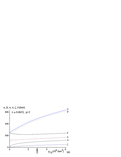
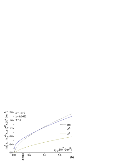
Figure 1: Panel: (a) The self-consistent parts $\alpha,\beta,\sigma,\vartheta,\zeta$ of the self-fields $A_{0}$, $B_{0}$, $W^{a=3}_{i=0}$, $W^{a=1}_{i=2}$–$W^{a=2}_{i=1}$ and $Z_{0}$, respectively, as functions of the electric charge density fluctuation $\varrho_{fQ}$($\vartheta\neq 0$, $\delta\neq 0$), Eq.(39). The self-consistent field $\delta$ of the self-field $\varphi_{f}$ as the function of $\varrho_{fQ}$($\vartheta\neq 0$, $\delta\neq 0$).
(b) The self-consistent parts $\left({\cal E}^{a\,A}_{a}\right)_{0}=g\,sin\Theta\,\alpha\,\vartheta$, (${\cal E}^{A}$), of the “electromagnetic electric ground fields” and $\left({\cal E}^{a\,Z}_{a}\right)_{0}=g\,cos\Theta\,\zeta\,\vartheta$, (${\cal E}^{Z}$), $a=1,2$ of the “weak electric ground fields” (see Eq.(34)-(35) and Eq.(37)) and $|\left({\cal B}^{3}_{3}\right)_{0}|=|-g\vartheta^{2}|$, ($|{\cal B}|$), of the absolute value of “electroweak magnetic ground field” as functions of $\varrho_{fQ}$.

Here, we notice only that the physical charge density fluctuation $\varrho_{fQ}$ (see Eq.(39)) for the EWbgfms configuration for different values of $p$ (see Table) converge for relatively small values of $\varrho_{fQ}$, i.e. for values of the charge density fluctuation $\varrho_{fQ}$ in the range of up to values approximately $10^{3}$ times bigger than those that correspond to the matter densities in the nucleon.

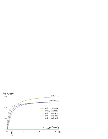
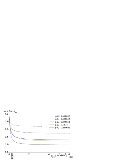
Figure 2: Panel: (a) The ratio of the observed electric charge density fluctuation $\varrho_{fQ}$ (see Eq.(44)) to the standard electric charge density fluctuation $\varrho_{fQ\;SR}$($\vartheta\neq 0$, $\delta\neq 0$) as the function of $\varrho_{fQ\;SR}$($\vartheta\neq 0$, $\delta\neq 0$).
(b) The ratio $sin\Theta/sin\Theta_{W}$ (see Eq.(49)) as the function of $\varrho_{fQ}$($\vartheta\neq 0$, $\delta\neq 0$).

Also, the ratio $\varrho_{fQ}/\varrho_{fQ\;SR}\rightarrow 1$ for $\varrho_{fQ\;SR}\rightarrow 0$ (see Figure 2a). As the result, all of the physical characteristics of the bgfms configurations for different values of $p$ (see Table) converge with $\varrho_{fQ}\rightarrow 0$ Dziekuje_Jacek_nova_2 . This can be noticed e.g. from the behavior of the ratio $sin\Theta/sin\Theta_{W}$ (Figure 2b) as a function of $\varrho_{fQ}$, where $\Theta$ is the modified mixing angle given by Eq.(49). On the other hand, $\varrho_{fQ}/\varrho_{fQ\;SR}\rightarrow C=const>1$ for $\varrho_{fQ\;SR}\rightarrow\infty$, where the value of $C$ depends both on $p$ and $\lambda$ (see Figure 2a). It can be noticed that the dependance of $C$ on the parameter $\lambda$ of the scalar fluctuation potential is stronger than on $p$. In principle, for bigger values of $\varrho_{fQ\;SR}$ the information on the true value of $\lambda$ should be extracted from the slope $C$ of the asymptote to the plot of $\varrho_{fQ}$ as the function of $\varrho_{fQ\;SR}$.

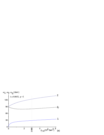
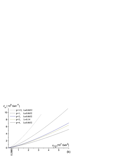
Figure 3: Panel: (a) The masses $m_{\tilde{A}}$, $m_{\tilde{Z}}$ and $m_{\tilde{\varphi}_{f}}$ of the gauge boson fields $\tilde{A}^{\mu}$ and $\tilde{Z}^{\mu}$ and of the scalar field fluctuation $\tilde{\varphi}_{f}$, respectively, as functions of the electric charge density fluctuation $\varrho_{fQ}$($\vartheta\neq 0$, $\delta\neq 0$).
(b) The energy density ${\cal E}_{st}(\varrho_{fQ})$, (63), of the EWbgfms configuration for boson ground fields calculated self consistently according to Eqs.(53)-(56) (for all values of $p\neq 0$ from the Table) as the function of $\varrho_{fQ}$.

From Eq.(29) and Eq.(43) (for $\vartheta\neq 0$), it can be noticed that fields $\tilde{W}^{+}$ and $\tilde{W}^{-}$ (see Eq.(61)), taken together as a pair of massive fields, become inside the EWbgfms configuration the massless self-fields that are coupled to the charge density fluctuations $\varrho_{fQ}\neq 0$ ($\varrho_{fQ\;SR}\neq 0$ and $\varrho_{fY}\neq 0$). The results for the dependance of the masses of $\tilde{A}$, $\tilde{Z}$ and $\tilde{\varphi}_{f}$ fields (see Eqs.(48) (47) and (52)) inside the EWbgfms configuration on the electric charge density fluctuation $\varrho_{fQ}$($\vartheta\neq 0$, $\delta\neq 0$) are presented in Figure 3a.

Let us notice that the expressions (47) for $m_{\tilde{Z}}^{2}$ and (48) for $m_{\tilde{A}}^{2}$ have a root. For a particular value of $p<1.388\approx 2\sqrt{\sin\Theta_{W}}$ and below some value of $\lambda=\lambda_{Z}$ (which depends on $p$), the expression $(m_{Z\;SR}^{2}+2g^{2}\vartheta^{2})^{2}-2(gg^{\prime}\delta\vartheta)^{2}$ under this root gets above some value of $\varrho_{fQ}$ the negative sign so that the EWbgfms configuration becomes unstable in the $\tilde{Z}$ and $\tilde{A}$ field sectors. Thus, for $p<1.388$ and a particular value $\lambda<\lambda_{Z}$, there is a value of $\varrho_{fQ}$ for which $m_{\tilde{A}}=m_{\tilde{Z}}$.
For example, for $p=1/2$ the limiting value $\lambda_{Z}\approx 0.2148$. Thus, e.g. for $\lambda=0.14<\lambda_{Z}$ this expression becomes negative above $\varrho_{fQ}\approx 1.767\times 10^{8}$ ${\rm GeV}^{3}$ (for which ${\cal E}_{st}(\varrho_{fQ})\approx 8.313\times 10^{10}$ ${\rm GeV}^{4}$). For $p=1/2$ and $\lambda=0.0652<\lambda_{Z}$ this expression becomes negative above $\varrho_{fQ}\approx 1.531\times 10^{7}$ ${\rm GeV}^{3}$ (for which ${\cal E}_{st}(\varrho_{fQ})\approx 3.456\times 10^{9}$ ${\rm GeV}^{4}$). Next, e.g. for $p=1$ the limiting value $\lambda_{Z}\approx 0.0297$. It will be shown in Section V that the value of $\varrho_{fQ}$ for a physically interesting EWbgfms configuration (e.g. the state $s2$ in Section V) (for which this instability might potentially appear) is smaller than the mentioned limiting value of $\varrho_{fQ}$. Moreover, above $p\approx 1.388$, and thus also from $p=3/2$ upwards, the discussed configurations do not possess this instability in the $\tilde{Z}$ and $\tilde{A}$ field sectors for all values of $\lambda$ and $\varrho_{fQ}$.

III.2 The mass of the EWbgfms configuration

The energy density given by Eq.(28) for stationary (st) solutions of the EWbgfms configuration for boson ground fields calculated self consistently according to Eqs.(53)-(56) as the function of $\varrho_{fQ}$ is equal to

$$\!\!\!\!\!\!\!\!\!\!{\cal E}_{st}(\varrho_{fQ}) = {\cal U}^{ef}_{f}(\vartheta\neq 0,\delta\neq 0)$$ (63)

$$({\rm with\;fields\;treated\;self\;consistently})\;.$$

The energy density ${\cal E}_{st}(\varrho_{fQ})$ increases both with $\varrho_{fQ}$ and $\varrho_{fQ\;SR}$. The plots of the dependance of ${\cal E}_{st}(\varrho_{fQ})$ for boson ground fields given by Eqs.(53)-(56) on the electric charge density fluctuation $\varrho_{fQ}$ are presented in Figure 3b (for values of $p\neq 0$ from the Table). We notice that from the point of view of ${\cal E}_{st}(\varrho_{fQ})$, the EWbgfms configurations fall into classes of $p$ that differ weakly with $\lambda$ inside a particular class (which is shown in Figure 3b for $p=2$ only).

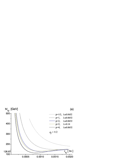
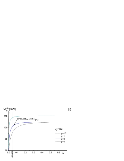
Figure 4: Panel: (a) The mass $M_{q_{f}=\pm 2}$ of the EWbgfms configuration as a function of the radius $r_{q_{f}}$ (for $p\neq 0$ from the Table and exemplary $\lambda$’s). The curves with $p\geq 1$ exhibit local minima. For example the minimal $M_{q_{f}=\pm 2}$ for $p=2$ and $\lambda\approx 0.0652$ is equal to $M^{min}_{q_{f}=\pm 2}=126.67$ GeV for $r_{q_{f}}\approx 0.00107\;fm$. The figures are plotted up to the values of $r_{q_{f}}$ smaller than $1/m_{\tilde{Z}}$ (see Figure 3a). For $p=1/2$ values of $\varrho_{fQ}$ are no bigger than $3.297\times 10^{7}$ ${\rm GeV^{3}}$ (for which $r_{q_{f}=2}\approx$ $0.000481\;fm$) as above it the configuration becomes unstable ($m_{\tilde{Z}}^{2}$ (47) and $m_{\tilde{A}}^{2}$ (48) become imaginary). For $p=1/2$ and for $\lambda>0.0119$ there are no EWbgfms configurations with local minimum of $M_{q_{f}}(r_{q_{f}})$.
(b) The minimal mass $M^{min}_{q_{f}}$ of the EWbgfms configuration as a function of $\lambda$. In the case of $p=1/2$, the thin wall approximation is not fulfilled and there are also no EWbgfms configurations with local minimum of $M_{q_{f}}(r_{q_{f}})$ for $\lambda>0.0119$; hence, we see the cut in the curve above this value (compare text under Figure 4a).

The matter electric charge fluctuation of an electrically charged EWbgfms configuration is equal to

$$q_{f}=\frac{4}{3}\,\pi\,r_{q_{f}}^{3}\,\varrho_{fQ}\;,$$ (64)

where $r_{q_{f}}$ is the “radius of the charge density fluctuation” in the thin wall approximation. The radius $r_{q_{f}}$ is the function of $\varrho_{fQ}$. The mass of the electrically charged EWbgfms configuration is equal to

$$\!\!M_{q_{f}}=\frac{4}{3}\,\pi\,r_{q_{f}}^{3}\;{\cal E}_{st}(\varrho_{fQ})\;\;\;\;{\rm and}\;\;\;\;M_{q_{f}}=\pm q_{f}M_{q_{f}=1}\;,$$ (65)

where because of the Pauli exclusion principle used for the fermionic fluctuations, we obtain that $q_{f}=\pm 1$ or $\pm 2$ only inside one droplet (except the cases that the consecutive fermionic fluctuations occupy their higher energy states). When the fermionic fluctuation (one or two in each bgfms configuration of fields) that plays the role of the matter source that induces boson ground fields was taken into account in the calculation of mass $M_{q_{f}}$, then its value would be changed by an order of the energy of this fermionic fluctuation. In this paper the energy of the fermionic fluctuation is neglected.
The functional dependence of the mass $M_{q_{f}}$ of a droplet of the EWbgfms configuration of fields (with charge fluctuation $q_{f}$) on $r_{q_{f}}(\varrho_{fQ})$ is presented in Figure 4a. It exhibits a minimum in $r_{q_{f}}$ (and also in $\varrho_{fQ}$) for some values of $p$. For instance (see Dziekuje_Jacek_nova_2 ), for $p=2$ and with $\lambda\approx 0.0652$, it has the minimal value $M_{q_{f}}=\pm q_{f}\times 63.335\;GeV$ at $\varrho_{fQ}=2.965\times 10^{6}\,{\rm GeV}^{3}$ ($\varrho_{fQ\;SR}=1.788\times 10^{6}\,{\rm GeV}^{3}$) and ${\cal E}_{st}(\varrho_{fQ})=1.878\times 10^{8}\,{\rm GeV}^{4}$ with the radius of the corresponding charge density fluctuation $r_{q_{f}}=q_{f}^{1/3}\times 0.000852\;fm$. In comparison, for a proton with a global electric charge $Q=1$, its electric charge radius $r_{Q}\approx 0.805\;fm$.
Finally, let us suppose that in the process, a droplet of the EWbgfms configuration with a particular $p\geq 1$ appears. This self-consistent charged EWbgfms configuration lies in the minimum of the function of mass $M_{q_{f}=2}$ v.s $\varrho_{fQ}$ (or $r_{q_{f}}$) (see Figure 4a). Its self-consistent (homogenous) self-fields are the solution of the equations of motion (100)–(102) and (105). If necessary, we will mark this minimal mass by $M^{min}_{q_{f}}$. This stationary state is the resonance via the weak interactions only, and can disintegrate through simultaneous decay or radiation of its constituent fields. The most interesting fact is that the closest configuration of fields is an electrically neutral Wbgfms configuration with the same mass. Because their masses are equal, hence their Breit-Weisskopf-Wigner probability density has a dispersion of the same order.

Note: From Figure 3b we see that ${\cal E}_{st}\longrightarrow 0$ as $\varrho_{fQ\;SR}\longrightarrow~{}0$ ($\varrho_{fQ}\longrightarrow~{}0$) for all of the values of $\lambda>0$ and $p\neq 0$ considered (see Table). For $\varrho_{fQ}\longrightarrow 0$ and for all of the considered values of $\lambda>0$ and $p\neq 0$ (see Table) from Eq.(28) and Eqs.(53)-(56), we also obtain

$$M_{q_{f}}\longrightarrow\pm\,q_{f}\,g\,v/2=\pm\,q_{f}\times 80.385\;{\rm GeV}\;,$$ (66)

where the sign “+” is for $q_{f}>0$ and sign “-” for $q_{f}<0$. Yet, as in this limit the EWbgfms configuration inside a droplet does not reproduce the uncharged SM configuration (for which $\varrho_{fQ}=0$), thus even for $q_{f}=\pm 1$ this bgfms configuration cannot be interpreted as the observed, well-known $W^{\pm}$ boson particle. Indeed, even if the charge density fluctuation tends in the limit to zero $\varrho_{fQ}\longrightarrow~{}0$ and thus we obtain $\vartheta\rightarrow 0$ and $\zeta\rightarrow 0$ for the ground fields of the $W^{+}-W^{-}$ pair and $Z$, respectively, yet, the result is that the self-consistent ground field $\alpha$ of $A_{0}$ is still non-zero in this limit (see Eq.(61) and Figure 1a) Dziekuje_Jacek_nova_2 . Therefore, the transition from the configuration of fields with $\varrho_{fQ}\neq 0$ ($\varrho_{fQ\;SR}\neq 0$ and $\varrho_{fY}\neq 0$) to the configuration with $\varrho_{fQ}=0$ (then with $\varrho_{fQ\;SR}=0$, $\varrho_{fY}=0$, $\alpha=0$, $\zeta=0$ and $\vartheta=0$) inside the droplet of the EWbgfms configuration is not a continuous one. Let us notice that in the double limit $\varrho_{fQ}\longrightarrow 0$ and $q_{f}\longrightarrow 0$, we obtain $M_{q_{f}}=0$.

IV Wbgfms configurations with $\varrho_{fZ\;SR}\neq 0$

From Eq.(49) it can be noticed that for $\vartheta=0$ the standard relation $tg\Theta=tg\Theta_{W}=\frac{g^{\prime}}{g}$ is held; hence, from Eqs.(39)-(II.1) it follows that $\varrho_{fZ}=\varrho_{fZ\;SR}$ and $\varrho_{fQ}=\varrho_{fQ\;SR}$. (The other possibility $tg\Theta=-\frac{g}{g^{\prime}}=-ctg\Theta_{W}$ obtained in this case from Eq.(49) is not a physical solution.)
Using Eqs.(37)-(38) we can rewrite the effective potential ${\cal U}^{ef}_{f}$ given by Eq.(28) for the ground fields in the following form

$$\!{\cal U}^{ef}_{f}(\zeta,\alpha,\delta)\!\! = \!\!\sqrt{g^{2}+g^{\prime 2}}\,\varrho_{fZ\;SR}\,\zeta+\frac{g\,g^{\prime}}{\sqrt{g^{2}+g^{\prime 2}}}\,\varrho_{fQ\;SR}\,\alpha$$ (67)

$$- \!\!\frac{1}{8}(g^{2}+g^{\prime 2})\,\delta^{2}\zeta^{2}+\frac{1}{4}\lambda\,(\delta^{2}-v^{2})^{2}\,.$$

For $\vartheta=0$ we can rewrite Eqs.(30)-(II.1) as follows

$$\varrho_{fQ\;SR}=0\;,$$ (68)

$$\frac{1}{4}\sqrt{g^{2}+g^{\prime 2}}\,\delta^{2}\,\zeta=\varrho_{fZ\;SR}$$ (69)

and

$$\lambda\,(\delta^{2}-v^{2})-\frac{1}{4}(g^{2}+g^{\prime 2})\,\zeta^{2}=0\;.$$ (70)

The relations (68)-(70) form the self-consistent part of the screening condition of the fluctuation of charges.
Note: Thus, according to Eq.(69), the non-zero weak charge density fluctuation $\varrho_{fZ\;SR}$ inevitably leads to the non-zero self-consistent field $\zeta$ of $Z_{\mu}$. The non-zero $\varrho_{fZ\;SR}$ also implies the non-zero self-consistent field $\delta\neq 0$ of the scalar fluctuation $\varphi_{f}$ (compare the Note below Eq.(56)).
Using Eq.(67) and equations (compare Eq.(33))

$$\partial_{\alpha}{\cal U}^{ef}_{f}=0\;,$$ (71)

and

$$\partial_{\zeta}{\cal U}^{ef}_{f}=\partial_{\delta}{\cal U}^{ef}_{f}=0\;,$$ (72)

the relations (68)-(70) can easily be checked.
Two nontrivial relations given by Eqs.(69) – (70) lead to the solution

$$\delta^{2}(\varrho_{fZ\;SR})=\frac{4\,\varrho_{fZ\;SR}}{\sqrt{g^{2}+g^{\prime 2}}\,\zeta}\;,$$ (73)

and

$$\zeta(\varrho_{fZ\;SR})=\frac{2}{3^{\frac{1}{2}}\,{\left(g^{2}+g^{\prime\,2}\right)}^{\frac{1}{2}}}$$ (74)

$$\times \frac{\,\lambda^{-\,\frac{1}{3}}{\left(3^{\frac{3}{2}}\,\varrho_{fZ\;SR}+{\sqrt{\,27\,{\varrho^{\,2}_{fZ\;SR}}+\lambda\,{v}^{6}\,}}\,\right)}^{\frac{2}{3}}-{v}^{2}}{\lambda^{-\,\frac{2}{3}}\,{\left(3^{\frac{3}{2}}\,\varrho_{fZ\;SR}+{\sqrt{\,27\,{\varrho^{\,2}_{fZ\;SR}}+\lambda\,{v}^{6}\,}}\,\right)}^{\frac{1}{3}}}\;,$$

where self-consistent fields $\zeta$ and $\delta$ are the functions of $\varrho_{fZ\;SR}$ only (see Figure 5a).

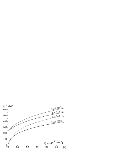
Figure 5: Panel: (a) The self-consistent fields $\zeta$ of $Z_{0}$ and $\delta$ of $\varphi_{f}$ as the function of the (standard) weak charge density fluctuation $\varrho_{fZ\;SR}(\vartheta=0,\delta\neq 0,\varrho_{fQ\;SR}=0$). In the limit $\varrho_{fZ\;SR}\longrightarrow 0$ the self-consistent ground fields tend to the uncharged values $\zeta=0$ and $\delta=v$.
(b) The masses $m_{\tilde{W}^{\pm}}$ (Eq.(90)), $m_{\tilde{Z}}$ (Eq.(88)) of the wavy part of $W^{\pm}_{\mu}$ and $Z_{\mu}$, respectively, and the mass $m_{\tilde{\varphi}_{f}}$ (Eq.(91)) of the wavy part of $\varphi_{f}$ inside the droplet of the Wbgfms configuration as the function of $\varrho_{fZ\;SR}(\vartheta=0,\delta\neq 0,\varrho_{fQ\;SR}=0$). In the limit $\varrho_{fZ\;SR}\longrightarrow 0$, these masses tend to the uncharged (i.e. for $\varrho_{fZ\;SR}=0$) values $m_{W^{\pm}}=g\,v/2$, $m_{Z}=\sqrt{g^{2}+g^{\prime 2}}\,v/2$ and $m_{\varphi_{f}}=\sqrt{2\lambda}\,v$, respectively.

Using Eqs.(23)-(26) and Eqs.(36)-(37), we can rewrite Eq.(20) for the self-consistent field $\alpha$ of $A_{\mu}$ in the form

$$A_{\mu}=(\alpha,0,0,0)\;.$$ (75)

From Eqs.(68)-(70) and (74)-(92) below it follows that $\alpha$ is not a dynamical variable. It corresponds to a nonphysical degree of freedom and can be removed by the gauge transformation $\alpha\rightarrow 0$. Thus, $U_{Q}(1)$ remains the valid symmetry group giving (see Eq.(37))

$$\alpha=\sigma sin\Theta_{W}+\beta cos\Theta_{W}=0\;.$$ (76)

Now, the self-consistent fields (20) can be rewritten as follows:

$$\left\{\begin{array}[]{lll}W^{1,2}_{\mu}=0\;\;,\;\;W^{3}_{i}=0\;,\\ W^{3}_{0}=-\beta\,ctg\Theta_{W}\;,\\ B_{0}=\beta\;,\\ B_{i}=0\;,\\ \varphi_{f}=\delta\;.\end{array}\right.$$ (82)

or in terms of physical fields

$$\left\{\begin{array}[]{lll}W^{\pm}_{\mu}=0\;\;,\;\;Z_{i}=0\;,\\ Z_{0}=\zeta\;\;,\;\;\;{\rm where}\;\;\;(\zeta=-\frac{1}{sin\Theta_{W}}\;\beta)\;,\\ A_{\mu}=0\;,\\ \varphi_{f}=\delta\;.\end{array}\right.$$ (87)

The appearance of the non-zero weak charge density fluctuation $\varrho_{fZ\;SR}$ and the self-consistent field $\zeta$ of the self-field $Z_{\mu}$ that is induced by it (see Eq.(74)) influences the masses of the wavy parts of the boson self-fields and of the scalar field fluctuation. Their squares inside a droplet of the Wbgfms configuration are, according to Eqs.(47)-(48), (51)-(52) (for $\vartheta=0$), equal to (see Figure 5b)

$$m_{\tilde{Z}}^{2}=\frac{1}{4}(g^{2}+g^{\prime 2})\delta^{2}\;,$$ (88)

$$m_{\tilde{A}}^{2}=0\;,$$ (89)

$$m_{\tilde{W}^{\pm}}^{2}=\frac{1}{4}g^{2}(\delta^{2}-4\,\zeta^{2}cos^{2}\Theta_{W})\;,$$ (90)

$$m_{\tilde{\varphi}_{f}}^{2}=\lambda\,(3\delta^{2}-v^{2})-\frac{1}{4}(g^{2}+g^{\prime 2})\,\zeta^{2}\;.$$ (91)

Thus the effective mass of the wavy part of the physical self-field $A_{\mu}$ is equal to $m_{\tilde{A}}=0$.

After putting the self-consistent ground fields calculated according to Eqs.(69)-(70) together with Eq.(68) into Eq.(67) the energy density for the stationary solution of the Wbgfms configuration, ${\cal E}_{st}(\delta,\varrho_{fZ\;SR})={\cal U}^{ef}_{f}(\delta,\;\varrho_{fZ\;SR};\;\vartheta=0,\;\varrho_{fQ\;SR}=0)$ is obtained Dziekuje_Jacek_nova_2

$${\cal E}_{st}(\delta,\varrho_{fZ\;SR})=2\,\frac{\varrho_{fZSR}^{2}}{\delta^{2}}+\frac{1}{4}\,\lambda\,(\delta^{2}-v^{2})^{2}\;\;\;\;$$ (92)

(with $\delta$ treated self consistently), which after using Eqs.(69) and (70) could also be rewritten as follows (see Figure 6)

$${\cal E}_{st}(\varrho_{fZ\;SR})=\frac{1}{2}\sqrt{g^{2}+g^{\prime 2}}\;\zeta(\varrho_{fZ\;SR})$$ (93)

$$\times \,\,\left(\varrho_{fZ\;SR}+\frac{1}{32\,\lambda}(g^{2}+g^{\prime 2})^{\frac{3}{2}}\,\zeta^{3}(\varrho_{fZ\;SR})\right)\,,$$

where the self-consistent ground field $\zeta=\zeta(\varrho_{fZ\;SR})$ is the function of $\varrho_{fZ\;SR}$ (see Eq.(74)).

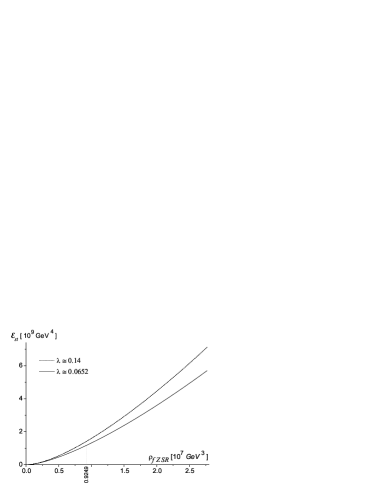
Figure 6: The energy density of the Wbgfms configuration ${\cal E}_{st}(\varrho_{fZ\;SR})={\cal U}^{ef}_{f}(\vartheta=0,\;\delta\neq 0,\;\varrho_{fQ\;SR}=0)$ (see Eq.(93)).

From Eqs.(90) and (73), it is clear that the appearance of $\varrho_{fZ\;SR}>0$ (so $\zeta>0$) leads to the instability in the $W^{\pm}_{\mu}$ sector only if

$$\zeta^{3}(\varrho_{fZ\;SR})>\frac{\sqrt{g^{2}+g^{\prime 2}}\,\varrho_{fZ\;SR}}{g^{2}}\;,$$ (94)

which is connected with the fact that then $m_{\tilde{W}^{\pm}}^{2}<0$ Dziekuje_Jacek_nova_2 . When the equality $\zeta^{3}(\varrho_{fZ\;SR})=\sqrt{g^{2}+g^{\prime 2}}\,\varrho_{fZ\;SR}/g^{2}$ is taken into account, we obtain the relationship between $\lambda_{max}$ and $\varrho_{fZ\,SR\,max}$, where $\lambda_{max}$ is the value of $\lambda$ and $\varrho_{fZ\,SR\,max}$ is the value of $\varrho_{fZ\;SR}$ for which we have $m_{\tilde{W}^{\pm}}^{2}=0$. The region of stable Wbgfms configurations with $\zeta\neq 0$ is on and below the $\varrho_{fZ\,SR\,max}(\lambda_{max})$ boundary curve (see Figure 7a).
For the weak charge density fluctuation $\varrho_{fZ\;SR}<\varrho_{fZ\;SR}^{limit}\equiv(g^{2}+g^{\prime\,2})\,v^{3}/(8\,g)$ $\approx 1.585\times 10^{6}\;$ ${\rm GeV}^{3}$, this configuration of fields is stable for an arbitrary $\lambda$ (see Figure 7a). For values of $\varrho_{fZ\;SR}$ bigger than $\varrho_{fZ\;SR}^{limit}$, the Wbgfms configuration is unstable for a given $\lambda$ above a certain value of $\varrho_{fZ\;SR}$, which is equal to

$$\varrho_{fZ\;SRmax}=\frac{8g^{2}\lambda^{\frac{3}{2}}\,(g^{2}+g^{\prime\,2})\,v^{3}}{\left[16g^{2}\lambda-(g^{2}+g^{\prime\,2})^{2}\right]^{\frac{3}{2}}}\;.$$ (95)

For $\lambda<\lambda_{limit}\equiv(g^{2}+g^{\prime\,2})^{2}/(16g^{2})\approx 0.0451$, the Wbgfms configuration is stable for all values of $\varrho_{fZ\;SR}$ (see Figure 7a).

IV.1 The mass of the Wbgfms configuration

Let us examine the mass of the droplet of the Wbgfms configuration induced by the non-zero weak charge density fluctuation $\varrho_{fZ\;SR}$

$$\!\!\!\!M_{i^{3}_{f}}=\frac{4}{3}\,\pi\,r_{i^{3}_{f}}^{3}\,{\cal E}_{st}(\varrho_{fZ\;SR})\;\;{\rm and}\;\;M_{i^{3}_{f}}=\pm\,i^{3}_{f}\,M_{i^{3}_{f}=1}\,,$$ (96)

where ${\cal E}_{st}(\varrho_{fZ\;SR})$ is given by Eq.(93) and the sign “+” is for $i^{3}_{f}>0$ and “-” for $i^{3}_{f}<0$. Because of the Pauli exclusion principle used for the fermionic fluctuations, only $i^{3}_{f}=\pm 1/2$ or $\pm 1$ (see Table) inside one droplet are possible (except in cases where the consecutive fermionic fluctuations occupy their higher energy states). Here, $r_{i^{3}_{f}}$ is the “radius of the weak charge density fluctuation” determined by the weak isotopic charge fluctuation inside the Wbgfms configuration in the thin wall approximation

$$i^{3}_{f}=\frac{4}{3}\,\pi\,r_{i^{3}_{f}}^{3}\,\varrho_{fZ\;SR}\;.$$ (97)

The radius $r_{i^{3}_{f}}$ is the function of $i^{3}_{f}$. The value of $|i^{3}_{f}|$ inside one droplet can possibly be more than 1 for the composite fermion fluctuation only composite_fermion .

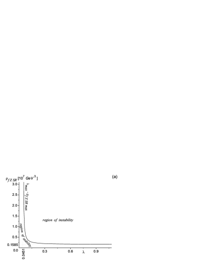
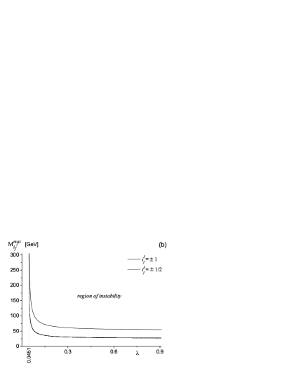
Figure 7: Panel: (a) The partition of the ($\lambda,\varrho_{fZ\;SR}$) plane into the regions of stability and instability of the Wbgfms configurations with $\varrho_{fZ\;SR}\neq 0$. The region of stable Wbgfms configurations lies on and below $\varrho_{fZ\,SRmax}(\lambda_{max})$ boundary curve, where $\lambda_{max}$ is the value of $\lambda$ and $\varrho_{fZ\,SRmax}$ is the value of $\varrho_{fZ\;SR}$ for which $m_{W^{\pm}}^{2}=0$. The limiting values $\varrho_{fZ\;SR}^{limit}\approx 0.1585\times 10^{7}\;$ ${\rm GeV}^{3}$ and $\lambda_{limit}\approx 0.0451$ are shown.
(b) The upper mass $M^{max}_{i^{3}_{f}}$ (according to the stability of the Wbgfms configuration in the ${W}^{\pm}$ sector) with $\varrho_{fZ\;SR}\neq 0$ as a function of $\lambda=\lambda_{max}$, where $m_{\tilde{W}^{\pm}}^{2}=0$ for points ($\lambda_{max}$, $M^{max}_{i^{3}_{f}}$) which lie on the curve. The region of possible Wbgfms configurations is on and below the $M^{max}_{i^{3}_{f}}(\lambda_{max})$ boundary curve. Two such curves, the first one for $i^{3}_{f}=\pm 1$ and the second one for $i^{3}_{f}=\pm 1/2$ are plotted. For $\lambda\rightarrow\infty$ $M^{max}_{i^{3}_{f}=\pm 1}\approx 52.277$ GeV and $M^{max}_{i^{3}_{f}=\pm 1/2}\approx 26.138$ GeV, respectively.

According to the stability of the Wbgfms configuration in respect of the $W^{\pm}$ sector, we can also obtain the upper limit $M^{max}_{i^{3}_{f}}$ for the value of the mass $M_{i^{3}_{f}}$. The region of the stability of possible Wbgfms configurations lies on and below the proper $M^{max}_{i^{3}_{f}}(\lambda_{max})$ boundary curve (see Figure 7b). Two such curves are presented, one for the function $M^{max}_{i^{3}_{f}=\pm 1}(\lambda)$ and the other for $M^{max}_{i^{3}_{f}=\pm 1/2}(\lambda)$. In principle, the value of $\lambda$ can be readout from the particular curve when the experimental value of the mass $M^{max}_{i^{3}_{f}}$ is known.

Note: It is not difficult to see that $\varrho_{fZ\;SR}\longrightarrow 0$ (which implies $\zeta\longrightarrow 0$ and $\delta\longrightarrow v$) entails ${\cal E}_{st}(\varrho_{fZ\;SR})\longrightarrow 0$ for the energy density (93) of the limiting Wbgfms configuration. The double limit $\varrho_{fZ\;SR}\longrightarrow 0$ and $i^{3}_{f}\longrightarrow 0$ is the only possibility for obtaining the weakly uncharged Wbgfms configuration. From Figure 7b it can be noticed that for the established value of $\lambda>\lambda_{limit}\approx 0.0451$ and with $i^{3}_{f}\longrightarrow 0$, the maximal mass $M_{i^{3}_{f}}$ of the Wbgfms configuration, which lies on the boundary curve $M^{max}_{i^{3}_{f}}(\lambda_{max})$, also tends to zero. Thus, in this case in the double limit $\varrho_{fZ\;SR}\longrightarrow 0$ and $i^{3}_{f}\longrightarrow 0$, the Wbgfms configuration becomes necessarily massless for $\lambda>\lambda_{limit}$ (for $\lambda\leq\lambda_{limit}$ this would be not necessarily the case).
At the same time, from Figure 5a-b we notice that for $\varrho_{fZ\;SR}\longrightarrow 0$, the Wbgfms configuration reproduces some characteristics of the uncharged $\varrho_{fZ\;SR}=0$ configuration, e.g. the masses of the (composite) boson fields and the lack of self-consistent gauge fields. Nevertheless, even for an infinitesimally small value of $\varrho_{fZ\;SR}$, the value of the self-consistent field $\delta$ is different from zero and tends in the limit to $v$. Thus, for $\lambda>\lambda_{limit}$ (which will be suggested later on) and for $\varrho_{fZ\;SR}\longrightarrow 0$, $i^{3}_{f}\longrightarrow 0$, the particles interacting with this massless Wbgfms configuration can perceive the fields that are inside a Wbgfms droplet with their SM values of couplings.

V The intersections of EWbgfms and Wbgfms configurations

Let us start with the electrically charged EWbgfms configuration with a matter electric charge fluctuation equal to $q_{f}=2$ (analysis for $q_{f}=-2$ would be the same) and a minimal mass $M^{min}_{q_{f}=2}$. Now, let us pose the question on the configuration of the nearest Wbgfms droplet with $\varrho_{fZ\;SR}\neq 0$ that arises after the decay of this minimal mass EWbgfms configuration with $\varrho_{fQ}\neq 0$. The solution with a particular value of $\lambda$ can be found as the point of the intersection of the function of the minimal masses $M^{min}_{q_{f}}(\lambda)$ of EWbgfms configurations (presented on Figure 4b) with the function of the maximal masses $M^{max}_{i^{3}_{f}}(\lambda)$ of Wbgfms configurations (presented on Figure 7b). Six such solutions can be seen in Figure 8a.

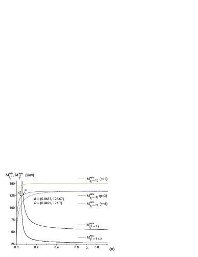
Figure 8: Panel (a): The intersections of the curves of the minimal masses $M^{min}_{q_{f}}(\lambda)$ of the EWbgfms configurations (presented on Figure 4b) with the curves of the maximal masses $M^{max}_{i^{3}_{f}}(\lambda)$ of the Wbgfms configurations (presented on Figure 7b).
(b): The EWbgfms configurations with the mass $M_{q_{f}=2}$ as a function of the radius $r_{q_{f}=2}$ and the Wbgfms configurations with the upper mass $M^{max}_{i^{3}_{f}=\pm 1}(r_{i^{3}_{f}})$ (according to the stability in the ${W}^{\pm}$ sector) as a function of the radius $r_{i^{3}_{f}=\pm 1}$. The “decomposition” of the particular solution $s1$ found in Figure 8a is shown. Two points, i.e. $s1_{q_{f}=2}$ with $M^{min}_{q_{f}=2}(r_{q_{f}})\approx 126.67$ GeV on the curve $M_{q_{f}=2}(r_{q_{f}})$ and $s1_{i^{3}_{f}=\pm 1}$ with the same mass on the curve $M^{max}_{i^{3}_{f}=\pm 1}(r_{i^{3}_{f}})$ correspond to one point $s1$ in Figure 8a. The right cut $r^{int}_{q_{f}=2}\sim 1/m_{Z}\approx 0.00196\;fm$ on the curve $M_{q_{f}=2}(r_{q_{f}})$ is connected with the thin wall approximation, whereas for the curve $M^{max}_{i^{3}_{f}=\pm 1}(r_{i^{3}_{f}})$ the maximal value of $r_{i^{3}_{f}=\pm 1}\approx 0.00105\;fm$ follows from the fact that for $\lambda\rightarrow\infty$ the limiting, lowest possible value of $\varrho_{fZ\;SR}$ for these upper mass configurations is equal to $\varrho_{fZ\;SR}^{limit}\approx 1.585\times 10^{6}\;$ $GeV^{3}$ (see Figure 7a).

The estimates obtained for the mass of the observed neutral state in the LHC experiment cms_1 ; cms_2 , atlas are in case of the CMS detector equal currently to $126.2$ $\pm 0.6$ (stat) $\pm 0.2$ (syst) GeV for its $ZZ^{(*)}\rightarrow 4\ell$ ($\ell=e$ or $\mu$) decay channel cms2 and in case of the ATLAS detector equal to $126.6$ $\pm 0.3$ (stat) $\pm 0.7$ (sys) GeV in the $\gamma\gamma$ channel or $123.5$ $\pm 0.8$ (stat) $\pm 0.3$ (sys) GeV in the $ZZ^{(*)}\rightarrow 4\ell$ channel atlas2 . Therefore, from the estimates obtained in the LHC experiment, only two solutions for the intersection of functions $M^{max}_{i^{3}_{f}}(\lambda)$ (one for $i^{3}_{f}=\pm 1/2$ and the other for $\pm 1$) with the function of the minimal masses $M^{min}_{q_{f}=2}(\lambda)$ for $p=2$ remain. These are the solutions $s1$ and $s2$, which are discussed below.

For the solution $s1$ in Figure 8a, we obtain $\lambda\approx 0.065187\approx 0.0652$ and $M^{min}_{q_{f}=\pm 2}=M^{max}_{i^{3}_{f}=\pm 1}\approx 126.67$ ${\rm GeV}$. Firstly, let us write down the characteristics of the electrically charged EWbgfms configuration with $\varrho_{fQ}\neq 0$ (see Eq.(61) and Figure 1a). Thus, the electric charge density fluctuation is equal to $\varrho_{fQ}=2.965\times 10^{6}$ ${\rm GeV}^{3}$ (compare Figure 2a) and the energy density (Figure 3b) is equal to ${\cal E}_{st}(\varrho_{fQ})\approx 1.878\times 10^{8}$ ${\rm GeV}^{4}$. For $q_{f}=2$ the radius of the electrically charged EWbgfms configuration is equal to $r_{q_{f}}\approx 0.00107\;fm$ (see Figures 4a and 8b). For $\varrho_{fQ}=2.965\times 10^{6}$ ${\rm GeV}^{3}$ the mass $m_{\tilde{Z}}\approx 124.128$ ${\rm GeV}$ inside the droplet of the EWbgfms configuration is the biggest one (see Figure 3a); hence, the interaction range $r^{int}_{q_{f}}$ inside the droplet is of the order $r^{int}_{q_{f}}\sim 1/m_{\tilde{Z}}\approx 0.00159\;fm$ and because the ratio $r_{q_{f}}/r^{int}_{q_{f}}\approx 0.675<1$, it is reasonable to use the thin wall approximation.
The other, i.e. the electrically neutral Wbgfms configuration of the solution $s1$ with the non-zero weak charge density fluctuation $\varrho_{fZ\;SRmax}\approx 9.249\times 10^{6}$ ${\rm GeV}^{3}$, has the energy density ${\cal E}_{st}(\varrho_{fZ\;SRmax})\approx 1.172\times 10^{9}$ ${\rm GeV}^{4}$ (Figure 6). For $i^{3}_{f}=\pm 1$ its radius is equal to $r_{i^{3}_{f}}\approx 0.000583\;fm$ (see Figure 8b). For this value of $\varrho_{fZ\;SRmax}$, the mass $m_{\tilde{Z}}=165.064$ ${\rm GeV}$ (see Figure 5b) is the biggest one ($m_{\tilde{\varphi}_{f}}=160.071$ ${\rm GeV}$); hence, the interaction range $r^{int}_{i^{3}_{f}}$ inside the droplet of the Wbgfms configuration is of the order $r^{int}_{i^{3}_{f}}\sim 1/m_{\tilde{Z}}\approx 0.0012\;fm$. Thus, because the ratio $r_{i^{3}_{f}=1}/r^{int}_{i^{3}_{f}}\approx 0.488<1$, it is reasonable to use the thin wall approximation.

The transition from the electrically charged EWbgfms configuration (state $s1_{q_{f}=2}$) to the uncharged Wbgfms configuration (state $s1_{i^{3}_{f}=\mp 1}$) is presented in Figure 8b. These two points are represented by one solution $s1$ on the $\lambda-M$ plane in Figure 8a. We interpret the electrically uncharged Wbgfms configuration represented by the point $s1_{i^{3}_{f}=\mp 1}$ as the candidate for the neutral state of the mass $\sim 126.5$ GeV recently observed in the LHC experiment.
Remark: In the presented paper, the masses of the states $s1_{q_{f}=+2}$ and $s1_{i^{3}_{f}}$ (or $s2_{q_{f}=+2}$ and $s2_{i^{3}_{f}}$) are equal. Yet, the mass splitting between the states $s1_{q_{f}=+2}$ and $s1_{i^{3}_{f}}$ (or $s2_{q_{f}=+2}$ and $s2_{i^{3}_{f}}$) could be of the 10 MeV order, which is in agreement with the value of the decay width of the $126.5$ GeV boson state observed in the LHC experiment Barger-Ishida-Keung ; CMS-do-Barger-Ishida-Keung (also Section V.1). Then, examples a11-b2 which follow, which have on their right hand sides the dielectron events plus neutrinos, are from this point of view not excluded by the present LHC experiment.

The examples of the processes connected with $s1$ are as follows.

For $s1_{q_{f}=+2}$ and $s1_{i^{3}_{f}=\pm 1}$, which are the leptonic states:
a11) $\;p+p\rightarrow(s1_{q_{f}=+2})+X+2\nu\;$ and then $\;(s1_{q_{f}=+2})\rightarrow(s1_{i^{3}_{f}=-1})+2\nu+2e^{+}$
a12) $\;p+p\rightarrow(s1_{q_{f}=+2})+X+2\nu\;$ and then $\;(s1_{q_{f}=+2})\rightarrow(s1_{i^{3}_{f}=+1})+2{\bar{\nu}}+2e^{+}$

For $s1_{q_{f}=+2}$ and $s1_{i^{3}_{f}=\pm 1}$, which are the barionic states:
a2) $\;p+p\rightarrow(s1_{q_{f}=+2})+X+({}^{\nu\ell^{+}}_{{\bar{\nu}}\ell^{-}})\;$ and then $\;(s1_{q_{f}=+2})\rightarrow(s1_{i^{3}_{f}=\mp 1})+2\nu+2e^{+}$.

Here $\ell$ is the electron or muon and $X$ signifies some jets.

For the solution $s2$ in Figure 8a, we obtain correspondingly $\lambda\approx 0.04977\approx 0.0498$ and $M^{min}_{q_{f}=\pm 2}=M^{max}_{i^{3}_{f}=\pm 1/2}\approx 123.7$ ${\rm GeV}$. The characteristics of the electrically charged EWbgfms configuration are as follows: $\varrho_{fQ}\approx 2.615\times 10^{6}$ ${\rm GeV}^{3}$, ${\cal E}_{st}(\varrho_{fQ})\approx 1.618\times 10^{8}$ ${\rm GeV}^{4}$ and for $q_{f}=2$ the radius of the droplet is equal to $r_{q_{f}}\approx 0.00112\;fm$. For this value of $\varrho_{fQ}$ the mass $m_{\tilde{Z}}\approx 121.940$ ${\rm GeV}$ is the biggest one; hence, the interaction range $r^{int}_{q_{f}}$ inside the droplet of the EWbgfms configuration is of the order $r^{int}_{q_{f}}\sim 1/m_{\tilde{Z}}\approx 0.00162\;fm$. Because $r_{q_{f}}/r^{int}_{q_{f}}\approx 0.692<1$, it is reasonable to use the thin wall approximation. The characteristics of the electrically neutral Wbgfms configuration are as follows: $\varrho_{fZ\;SRmax}\approx 5.477\times 10^{7}$ ${\rm GeV}^{3}$ with ${\cal E}_{st}(\varrho_{fZ\;SRmax})\approx 1.355$ $\times 10^{10}$ ${\rm GeV}^{4}$ and for $i^{3}_{f}=\pm 1/2$ we obtain $r_{i^{3}_{f}}\approx 0.000256\;fm$. For this value of $\varrho_{fZ\;SRmax}$, the mass $m_{\tilde{Z}}=298.621$ ${\rm GeV}$ is the biggest one ($m_{\tilde{\varphi}_{f}}\approx 253.036$ ${\rm GeV}$); hence, $r^{int}_{i^{3}_{f}}\sim 1/m_{\tilde{Z}}\approx 0.000661\;fm$. Because $r_{i^{3}_{f}}/r^{int}_{i^{3}_{f}}\approx 0.387<1$, it is reasonable to use the thin wall approximation. The exemplary processes for the $s2$ case (see Figure 8a) are as follows.

For $s2_{q_{f}=+2}$ and $s2_{i^{3}_{f}=\pm 1/2}$, which are the leptonic states:
b11) $\;p+p\rightarrow(s2_{q_{f}=+2})+X+2\nu\;$ and then $\;(s2_{q_{f}=+2})\rightarrow(s2_{i^{3}_{f}=-1/2})+\nu+2e^{+}$
b12) $\;p+p\rightarrow(s2_{q_{f}=+2})+X+2\nu\;$ and then $\;(s2_{q_{f}=+2})\rightarrow(s2_{i^{3}_{f}=+1/2})+{\bar{\nu}}+2e^{+}$

For $s2_{q_{f}=+2}$ and $s2_{i^{3}_{f}=\pm 1/2}$, which are the barionic states:
b2) $\;p+p\rightarrow(s2_{q_{f}=+2})+X+({}^{\nu\ell^{+}}_{{\bar{\nu}}\ell^{-}})$ and then $\,(s2_{q_{f}=+2})\rightarrow(s2_{i^{3}_{f}=\mp 1/2})+2\nu+2e^{+}$.

Some of the above processes look like the lepton number violation (i.e. a12, b11 and b12), but if $s_{q_{f}}$ and $s_{i^{3}_{f}}$ are leptonic states, they are not really of this type.
If the LHC state can be either a barionic or leptonic one, then the $q_{f}=2$ possibility is chosen only on the basis of the observed mass. Next, if the droplets of the bgfms configurations are leptonic, then the states with $|q_{f}|>2$ are (by the Pauli exclusion principle) possible only if the consecutive fermionic fluctuations are in higher energy states. Nevertheless, in both cases, the barionic and leptonic, the particular function $M^{min}_{q_{f}}(\lambda)$ for the EWbgfms configurations with $|q_{f}|>2$ intersects with the functions $M^{max}_{i^{3}_{f}}(\lambda)$ of the Wbgfms configurations for higher masses and these solutions have not yet been observed in an LHC experiment.
Let us consider the case when the bgfms configurations $s_{q_{f}}$ and $s_{i^{3}_{f}}$ are occupied by two (electrically charged and uncharged, respectively) fermionic fluctuations with opposite spin projections. In addition to the scalar fluctuation $\varphi_{f}$, there are four gauge self-fields inside the configuration given by Eq.(61) and three inside the configuration given by Eq.(87)). Thus, for the particular configuration of the ground fields given by Eq.(61), its EWbgfms $s_{q_{f}}$ droplet can have spin zero (and zero to four for its excitations). Meanwhile, for the particular configuration of the ground fields given by Eq.(87), its Wbgfms $s_{i^{3}_{f}}$ droplet can have spin zero (and zero to three for its excitations helicity_of_W_Bilenkii ; helicity_of_W_Gounaris ; helicity_of_W_Fleischer ; helicity_of_W_Bella ). Indeed, because $s_{i^{3}_{f}=\pm 1}$ is the ground state configuration, hence the self-consistent field $Z_{0}$ exists only inside its droplet (see Eq.(87)), which belongs to the spin zero subspace of the 3-dimensional rotation group. Thus, the $s_{i^{3}_{f}=\pm 1}$ ground configuration of fields, which consists of two opposite spin fermionic fluctuations, the scalar fluctuation $\varphi_{f}=\delta$ and spin zero $Z_{0}=\zeta$, has a spin equal to zero. (When boosted the $Z$ self-field is longitudinally polarized, i.e. its spin is equal to one with a spin projection equal to zero.) Next, from the point of view of the possible value of the spin of the Wbgfms configuration, considerations similar to the ones above (for two fermionic fluctuations) lead to the conclusion that states $s_{i^{3}_{f}=\mp 1/2}$ in b11, b12 and b2 with quantum numbers for fermionic fluctuation like those in the Table are excluded by the LHC experiment as they consist of one fermionic fluctuation only thus having a half spin value.
We see that only cases a11, a12 and a2 are possible and thus the present day experiments have selected the state $s1_{i^{3}_{f}=\mp 1}$ with mass $M^{max}_{i^{3}_{f}=\mp 1}\approx 126.67$ ${\rm GeV}$ for $\lambda\approx 0.0652$ and rejected the state $s2_{i^{3}_{f}=\mp 1/2}$ with mass $M^{max}_{i^{3}_{f}=\mp 1/2}\approx 123.7$ ${\rm GeV}$ for $\lambda\approx 0.0498$. However, the basic fields that induce the bgfms configurations of fields are (in this model) the fermionic fluctuations; hence, one could think that the states $s_{q_{f}=2}$ and $s_{i^{3}_{f}=\mp 1}$ are leptonic states (think of some models of a neutron in which the neutron is a composition of a barionic proton and a fermionic electron Santilli_1 ; Santilli_2 ). In this case, only the possibility of a leptonic state $s1_{i^{3}_{f}=\mp 1}$ remains, which is exemplified by processes a11 and a12. Otherwise, the barionic states exemplified by processes a2 remain with the configuration $s1_{i^{3}_{f}=\mp 1}$ suggested as the solution for the state observed in the LHC experiment.
In Figure 8a three pairs of neighbouring solutions can be noticed. Nevertheless, whether besides the experimentally noticeable state $s1_{i^{3}_{f}=\pm 1}$, the neighbouring solution $s2_{i^{3}_{f}=\mp 1/2}$ together with the remaining ones have been also observed cms3_1 ; cms3_2 ; cms3_3 ; cms3_4 as more shallow resonances and not as the statistical flukes in the data only, remains an open question. The reason is that in such a case $\lambda$ gains two additional indexes, i.e. $\lambda\rightarrow\lambda_{p,i^{3}_{f}}$, where the electric charge to hypercharge ratio index $p$, Eq.(62), numbers the EWbgfms configurations and the weak isotopic charge $i^{3}_{f}=\mp\frac{1}{2},\mp 1$ numbers the Wbgfms ones.
Thus, in Figure 8a for each $p$, where $p=1,2$ and 4, one pair ${s_{i^{3}_{f}=\mp 1/2}\choose\!\!\!s_{i^{3}_{f}=\mp 1}}$ of the neighbouring solutions:

$$\!\!\!\!\!\!\!\!\!\!\!\!\!\!\!\!\!\!\!\!\!\!\!\!\!\!\!\!\!\!\!\!{(0.0512,108.79)\choose(0.0705,114.91)}\,,\;$$

$${(0.0498,123.7)\choose(0.0652,126.67)}\;\; {\rm and} \;\;{(0.0484,146.33)\choose(0.0593,147.4)}\,,$$ (98)

respectively, can be noticed, where for each of the six solutions the values of $\lambda$ and $M^{max}_{i^{3}_{f}}$ [${\rm GeV}$] are given.
The central column in Eq.(V) is ${s2_{i^{3}_{f}=\mp 1/2}\choose\!\!\!s1_{i^{3}_{f}=\mp 1}}$. It is easy to notice that the algebraic mean of the mass of two central neighbouring solutions $s1_{i^{3}_{f}=\pm 1}$ and $s2_{i^{3}_{f}=\mp 1/2}$ is equal to 125.185 GeV. This value is consistent with the mean mass of the configurations observed in the first run of the LHC experiment (with higher than $5\sigma$ significance of the observed excess over the expected background PDG-2014-2015 ). Yet, it has to be also noticed that the values in the third column in Eq.(V) lie in the vicinity of the events recorded in the CMS experiment at a mass of approximately 145 GeV with a statistical significance of $\sim 3\sigma$ above background expectations cms3_1 ; cms3_3 ; Khallil-Moretti .

Finally, it is not difficult numerically to check that for all Wbgfms configurations that lie on their boundary curve $M^{max}_{i^{3}_{f}}(\lambda_{max})$ and have a particular value of the weak isotopic charge fluctuation $i^{3}_{f}$, the relation

$$\frac{4}{3}\,\pi\,r_{i^{3}_{f}}^{3}\,\delta^{3}/(3\,\pi)\approx|i^{3}_{f}|\;$$ (99)

is fulfilled (up to the fourth digit after the decimal point). The mass of the droplet calculated with $\delta$ obtained from the perfect equality in Eq.(99) with the (non self-consistent) use of Eq.(63) agrees with $M^{max}_{i^{3}_{f}}$ up to the seventh digit after the decimal point. Thus, the relation (99) is also fulfilled by the configurations $s1_{i^{3}_{f}=\mp 1}$ (and e.g. $s2_{i^{3}_{f}=\mp 1/2}$ also). The Wbgfms configuration $s1_{i^{3}_{f}=\mp 1}$ is the successor of the EWbgfms configuration $s1_{q_{f}=2}$. In Figure 8a these configurations overlap. Both have a mass equal to $126.67$ GeV, which (besides the spin zero) has been interpreted above as the signature of the LHC state. In this way both the charge $q_{f}=2$ and $i^{3}_{f}=\pm 1$ are discreetly chosen. Thus, it is suggested by Eq.(99) that in the one parametric $\varrho_{fZ\;SR}\neq 0$ case (see Eqs.(73)-(74)), the quantization $i^{3}_{f}=\pm 1$ is an artefact of the self-consistency conditions given by Eqs.(69)-(70). The analysis of condition (99) will be discussed in a following paper.

V.1 The decay of the $s1_{i^{3}_{f}=\mp 1}$ droplet

In the full-self consistent field theory, fields have the same type of couplings as their counterparts in the perturbative quantum field theory. This is the case of e.g. the self-consistent electrodynamics and one of its outcomes is the derivation of the Lamb shift by Barut and Kraus bib_B-K-1 . Although the presented CGSW model treats the self-consistent field and the wave self-field of excited states differently, a self-field is in reality one object (on the ground state, i.e. in the droplet of a bgfms configuration, only self consistent fields are present). Thus, both the self-consistent field and the wave self-field in CGSW have the same type of couplings as their counterparts in the GSW model.
The self-consistent electrically uncharged Wbgfms configuration $s1_{i^{3}_{f}=\mp 1}$ is the resonance via the weak interactions only and can disintegrate through the simultaneous decay or radiation of its constituents. In a droplet of a Wbgfms configuration of fields induced by $\varrho_{fZ\;SR}\neq 0$ (with $\varrho_{fQ\;SR}=0$), the self-consistent fields $\varphi_{f}$ and $Z$ (see Eq.(87)) are present in addition to the background fermionic fluctuations. Then, only $\delta$ of $\varphi_{f}$ and the time component $\zeta$ of $Z$ are different from zero. (Due to $\varrho_{fQ\;SR}=0$ and $m_{A}=0$, the electromagnetic self-field $A$ is totally absent even in the excitation; however, the pair $W^{+}-W^{-}$ of the self-fields can appear in the excitation.) The self-consistent fields are the initial ones that take part in the decay of the Wbgfms configuration. For each initial self-consistent field the calculation of the coherent transition probability is performed separately (i.e. for $\varphi_{f}=\delta$ and $Z_{0}$) and then the decay of the droplet of the Wbgfms configurations is calculated in accordance with the following scenario. Firstly, there appears the decay of the coupling of the self-consistent field $\zeta$ of $Z_{\mu}$ to the basic fermionic field followed by the decay of $\zeta$ (which is very rapid in SM). Then, (for $\varrho_{fZ\;SR}\longrightarrow 0$, $i^{3}_{f}\longrightarrow 0$ and $\lambda>\lambda_{limit}$) the fields configuration of the droplet decays (see Note in Section IV.1). In this limit, the particles interacting with the configuration can perceive, with the SM values of couplings, fields that are inside the droplet. This leads to the decay of the self-consistent field $\delta$ of the scalar fluctuation $\varphi_{f}$ with the decay rate of the same order as predicted for the SM Higgs particle. Thus, roughly speaking, the decay width of the Wbgfms configuration shall be of the order of a few MeV. Finally, only longer-lived particles are detected in the detector.

V.2 Transparency of the uncharged bgfms configuration to electromagnetic radiation

In Section IV it was noted that the effective mass $m_{A}$ of the electromagnetic self-field $A$ inside the droplet of an electrically uncharged Wbgfms configuration is equal to zero. Although the electromagnetic self-field is totally absent in this bgfms configuration (see Section IV), zeroing of the effective mass and $\varrho_{fQ}=0$ are important for the photons that are external ones (see Introduction). The reason is that the formal form of the equation of motions (100)-(102) is also true for the external gauge fields penetrating the discussed bgfms configuration. Thus, the Wbgfms configuration is transparent for the external electromagnetic radiation.
Now, let us suppose that the matter is extremely dense, as could happen in the mergers of neutron stars. Then the difference between the inward structure of the nucleon and the inward structure of the droplet of the Wbgfms configuration may be a supporting impulse to initiate the relativistic shock. That is, the abrupt transition of the neutron matter during the collapse of star mergers could cause the transition to matter of Wbgfms droplets, which are transparent to the gamma radiation that is produced within the gamma-ray bursts (GRB) explosion. This can lead to the appearance of an alternative source of energy that can help the gamma-ray burst MarekJacek . This would also be the reason for the recently observed lack of correlations between gamma-ray bursts and the neutrino fluxes (present in the standard model dziekuje_za_DLS2 and) directed from them bursts_lack_neutrino_LoSecco ; bursts_lack_neutrino_Abbasi ; bursts_lack_neutrino_Taboada ; bursts_lack_neutrino_IceCube .

VI Conclusions

The aim of this paper was to examine homogeneous self-consistent ground state solutions in the CGSW model Dziekuje_Jacek_nova_2 . It is an effective one as is the GSW model which is its quantum counterpart. It is assumed that if the ground state of the configuration of the self-fields induced by extended (non-bosonic) charge fluctuations appears JacekManka , then this forces us to describe the physical system inside its droplet in the manner of classical field theory.
Let us summarize the results presented in this paper. The discussed model is homogeneous on the level of one droplet (thus the thin wall approach is used). The homogeneous configurations of the gauge ground self-fields $W^{\pm}_{1,2}$, $Z_{0}$ and $A_{0}$ and the scalar field fluctuation $\varphi_{f}$ in the presence of a spatially extended homogeneous basic fermionic fluctuation(s) that carries the nonzero charges were examined. The ground fields penetrate the whole spatially extended fermionic fluctuation(s) and in their presence the electroweak force generates “the electroweak screening fluctuation of charges” according to Eqs.(29)-(II.1).
In general, we notice two physically different configurations of the fields. When a matter source has the charge density fluctuation $\varrho_{fQ\;SR}\neq 0$, then classes diffrent-classes of the ground fields configurations EWbgfms (with $\vartheta\neq 0$ and $\delta\neq 0$) that are induced by this source exist (see Section III). The mass (65) of a droplet of this configuration of field was determined for the value of the matter electric charge fluctuation equal to $q_{f}$, (64). The EWbgfms configurations lie on the $M_{q_{f}}(\varrho_{fQ})$ curves (see Figure 4a) or equivalently on the ${\cal E}_{st}(\varrho_{fQ\;SR})$ curves only (see Figure 3b). For the particular value of $p$, the functions $M_{q_{f}}(\varrho_{fQ\;SR})$, (65), and their minima $M^{min}_{q_{f}}$ depend on $\lambda$ (see Figure 4a).
Inside the droplet, both the appearance of the mass of the (non self consistently treated) wavy self-field $\tilde{A}_{\mu}$ and the modification of the masses of the wavy self-fields $\tilde{W}^{+}_{\mu}-\tilde{W}^{-}_{\mu}$, $\tilde{Z}_{\mu}$ and also the scalar fluctuation field $\varphi_{f}$ are caused due to the existence of the self-consistent fields (see Section II.1) and due to the screening effect of the fluctuation of charges formulated by Eqs.(29)-(II.1). Then, the obtained masses are used in order to estimate the thin wall approximation range. A more complete description of the EWbgfms configurations, e.g. the dependance of the observed charge density fluctuation $\varrho_{fQ}$ on $\varrho_{fQ\;SR}\neq 0$ and the modification of the mixing angle $\Theta$, (49), with a change of $\varrho_{fQ}$ and the stability of the EWbgfms configurations is given in Section III.
When the weak charge density fluctuation $\varrho_{fZ\;SR}\neq 0$ (and $\varrho_{fQ\;SR}=0$) then the electrically uncharged, weakly charged Wbgfms configurations with $\vartheta=0$ and $\delta\neq 0$ and the ground self-field $Z_{0}=\zeta\neq 0$ can exist (see Section IV). The region of the stable (for the sake of the $W^{\pm}$ sector) Wbgfms configurations lies on and below the $\varrho_{fZ\,SRmax}(\lambda_{max})$ boundary curve (see Figure 7a). For the particular value of ${i^{3}_{f}}$, (97), the function $\varrho_{fZ\,SRmax}(\lambda_{max})$ gives the function $M^{max}_{i^{3}_{f}}(\lambda_{max})$, which divides the plane $\lambda\times M_{i^{3}_{f}}$ of all Wbgfms configurations into the stability and instability regions (see Figure 7b). A more complete description of the Wbgfms configurations can be found in Section IV.

Previously, in Dziekuje_Jacek_nova_2 it was found that for $\lambda=1$ and for $p=2$ a shallow minimum of the mass of the EWbgfms configuration droplet equal to $M^{min}_{q_{f}}\approx\pm q_{f}\times 66.7464\;GeV$ appears. At that time the expectation was that the appearance of such bgfms configurations might be theoretically possible in the very dense microscopic objects that are created in heavy ion collisions ion-collisions . In the present paper in Section V, the complete characteristics of two such bgfms configurations $s1_{q_{f}=2}$ and $s2_{q_{f}=2}$ were given. We only remind the reader that for the zero spin $s1_{q_{f}=2}$ state (realized for $\lambda\approx 0.0652$) the mass of the EWbgfms droplet equal to $M^{min}_{q_{f}=2}\approx 126.67$ ${\rm GeV}$ was obtained. The physical realization of the other EWbgfms $s2_{q_{f}=2}$ state (at least as far as its mass is taken into account) is doubtful, as the fields configuration inside the droplet of its electrically neutral Wbgfms successor $s2_{i^{3}_{f}=\mp 1/2}$ is induced by one fermionic fluctuation only thus having a half spin value, which is less consistent with the observations reported in the LHC experiment spin_in_LHC_Miller_1 ; spin_in_LHC_Miller_2 , spin_in_LHC_Gao ; spin_in_LHC_Englert ; spin_in_LHC_Djouadi ; spin_in_LHC_Ellis . As it was previously mentioned only, the algebraic mean of the mass of the central solutions $s1$ and $s2$, i.e., 126.67 GeV and 123.7 GeV, respectively, is equal to 125.185 GeV.
Thus, the remaining, zero spin EWbgfms state $s1_{q_{f}=2}$ is the configuration in the minimum of the $M_{q_{f}}(r_{q_{f}})$ curve for $p=2$, $q_{f}=2$ and with $\lambda\approx 0.0652$ (see Figure 4a). It lies on the $M^{min}_{q_{f}=2}(\lambda)$ curve at the point of its intersection with the boundary curve $M^{max}_{i^{3}_{f}=\mp 1}(\lambda=\lambda_{\max}\approx 0.0652)$ (see Figure 8a). The intersection point is interpreted as the one that corresponds to the transition of the electrically charged EWbgfms configuration $s1_{q_{f}=2}$ to the electrically uncharged zero spin Wbgfms state $s1_{i^{3}_{f}=\mp 1}$, which has the mass $M^{max}_{i^{3}_{f}=\mp 1}\approx 126.67$ ${\rm GeV}$, as can be seen in Figure 8b. In Section V it was argued that the configuration $s1_{i^{3}_{f}=\mp 1}$ corresponds to the LHC $\sim 126.5$ GeV zero spin state. This physically interesting solution, which is discussed in the present paper, has not been found before (see Figure 8a).
In this paper it was also noted that for both the EWbgfms and Wbgfms configurations the non-zero charge fluctuations (fundamentally $\varrho_{fY}$) imply a non-zero value of the self-consistent field $\delta\neq 0$ of the scalar fluctuation $\varphi_{f}$ (compare Notes in Section III below Eq.(56) and in Section IV below Eq.(70)). Thus, in the more fundamental theory, the self-consistent field $\delta$ could be a secondary quantity. Because for both EWbgfms and Wbgfms configurations (for which $\varrho_{fY}\neq 0$), we find that the limit $\varrho_{fY}\rightarrow 0$ implies $\delta\rightarrow v$ thus a derivative meaning for the parameter $v$ of the scalar fluctuation potential may also be suggested.
Finally, if Wbgfms state $s1_{i^{3}_{f}=\mp 1}$ is interpreted as the LHC $\sim 126.5$ GeV one, then this means that the value of $\lambda=\lambda_{max}\approx 0.0652$, which is the constant parameter of the CGSW model, is a little bit bigger than the limiting stability value $\lambda^{limit}=g^{2}/(16\;cos^{4}\Theta_{W})\approx 0.0451$ (see Section IV and Figures 7a-b). A bgfms state exists for $\lambda\approx 0.0652$ only (although other specific values of $\lambda$ are possible in an extension of the model, see Eq.(V)). Therefore, a Wbgfms configuration of fields with $\varrho_{fZ\;SR}$ bigger than $\varrho_{fZ\;SRmax}\approx 9.249\times 10^{6}$ ${\rm GeV}^{3}$ (which is the density for $s1_{i^{3}_{f}=\mp 1}$ state, calculated in accordance with Eq.(95)) lies above the $s1_{i^{3}_{f}=\mp 1}$ state in the instability region (see Figure 7), and is unstable in the $W^{\pm}$ sector. Therefore, as was suggested in Dziekuje_Jacek_nova_2 , it radiates to the states with $\varrho_{fZ\,SR}\leq\varrho_{fZ\,SRmax}$ or decays into stable particles, i.e. photons, leptons, hadrons and neutrinos, as was described in Section V.1.

The non-linear self-consistent classical field theory is inherently connected with the existence of the self-field Barut-1 ; Barut-2 ; Barut-3 ; Barut-4 , B-Nonlinear-1 ; B-Nonlinear-2 , bib_B-K-1 coupled to the basic field (fluctuation). For example, in the perturbative QED the classical self-field of the electron fluctuation is completely absent and it comes back in via a separate quantized radiation field “photon by photon”. Meanwhile, in the self-consistent classical field concept, the whole self-field is put in from the beginning. It is free of the idea of the quantum field theory vacuum (state) Nedelko:2014sla and the virtual pair creation.
The self-field concept was previously used with great success in the Abelian case e.g. in order to compute nonrelativistic Lamb shifts and spontaneous emission spontaneous-1 ; spontaneous-2 , the Lamb shift (obtained iteratively) relativ_Lamb , spontaneous emission in cavities bib_B-D and long-range Casimir-Polder van der Waals forces Casimir . These analyses follow the work of Jaynes and Milonni Jaynes-1 ; Jaynes-2 ; Jaynes-3 , Milonni and the even earlier 1951 paper of Callen and Welton Callen-Welton on the fluctuation dissipation theorem, which showed that there is an intimate connection between vacuum fluctuations and the process of radiation reaction. The existence of one implies the existence of the other.
The linear Dirac equation alone with e.g. the electron wave function in the presence of the (external to it) Coulomb field leads to wave mechanical solutions for the ground and excited states of the electron in an atom (see Introduction). The mathematics of the non-linear Dirac equation for the basic field fluctuation, which follows from the coupled Maxwell and linear Dirac equations for this fluctuation and its electromagnetic self-field is quite different. In general, the mathematics of the self-consistent field theory is interested in a proper set of partial differential equations, which are then solved self consistently in such a way that all degrees of freedom are removed. What remains is one particular state of the system.
Remark: For example, the self-consistent solution of the couple: the Dirac equation and classical Maxwell equations will give a real photon that is a “lump of electromagnetic substance” (without Fourier decomposition Dziekuje_za_channel ; Dziekuje_za_skrypt as is suggested from recent experiments Roychoudhuri ) as the reflection of the coupling to the Dirac equation. If we pull back from this particular solution forgetting about the primary Dirac equation then what remains are not the classical Maxwell equations for the classical electromagnetic field but equations that act on the space of possible photonic states. QED with the field operator and the Fock space have to be the non-self-consistent reflection of this construction (if only the Fourier decomposed frequencies of the light pulse represent actual optical frequencies, which has recently been questioned by light beam experiments Roychoudhuri ). (Compare the self-consistent pair of equations (69)-(70) with the non-self-consistent Eq.(99)).
The merits of the thought that is behind this procedure is the self consistency of the solution. The further we are from this precise self-consistent solution, the more numerous a set of differential equations remains to be solved but the set of equations that are already solved determines the types of the equations which remain and the properties of the fields that are ruled by them.
The self-field is small for atomic phenomena and therefore the description of the basic field fluctuation via the linear Dirac equation may work approximately, which follows from the fact that the non-linear terms are small and can be treated as perturbations. Nevertheless, the QED prevailed, mainly because of the successes in the scattering phenomena.
Yet, the self-field is not always small and there is another region where the non-linear terms dominate B-Nonlinear-1 ; B-Nonlinear-2 . The present paper reflects such a situation, since for the bgfms configuration of fields, the energy of the host fermionic fluctuation is assumed to be minute in comparison to the obtained mass of the bgfms droplet. Thus, the main theoretical subject of this paper was the self-consistent description of the configuration of electroweakly interacting self-fields that are induced by a charge density fluctuation(s) with the internal extended wave structure inside one droplet. Thus, the CGSW model is the type of “a source theory” that considers all self-fields and scalar field fluctuations as “derived” from the source of the fluctuations of charges. The quotation marks mean that the self-consistent fields are not absent - they are only self consistently derived from the basic fluctuations fields to which they are coupled via the screening condition of the fluctuation of charges (29)-(II.1).

In the presented CGSW model of the bgfms configuration of fields induced by the basic matter field fluctuation(s), the droplet is like the whole particle. This is connected with the fact that (besides the fact that the energy of the fermionic fluctuation is ignored) any fermionic fluctuation which “stretches” the droplet is like a whole fermion. Thus, our droplet of the bgfms configuration is like “a parton”. This is definitely not the most general case.
The indispensable need for the development of a more general approach is seen from the self-consistent model of the configuration of fields induced by the electronic charge fluctuation used in the Lamb shift explanation, where the energy of the electronic fluctuation is ignored (not to mention the ground and excited states of the electron, which are obtained in the anticipation by the formalism of the wave mechanics for the total electron wave function that is treated non-self consistently). Therefore, let us assume that there is an object in which the fluctuation of the fermionic charge does not exist by itself but needs a globally extended fermionic charge of which it is the disturbance only. With such approach, one is obliged to define and find the mass of the configuration of fields induced by the globally extended charge together with its fluctuation(s) (extended globally or locally). In doing this, one should focus on neither the wave mechanics (or quantum mechanics) nor on the self-consistent field theory of fluctuations (or quantum field theory) but on the theory of the complete inner structure of one particle. Otherwise, the model gets into the composition of “a particle” from “partons”, which is a kind of “planetarianism” and seemingly because of this e.g. quantum chromodynamics (QCD) is the theory without final fundamental success nucleac_spin_crisis , as was expressed in Heyde : “… all spin parts $\left[{\rm of\;the\;nucleon}\right]$ have to add to $\frac{1}{2}$ which is incredible in the light of the present day experiments. This may indicate that some underlying symmetries, unknown at present, are playing a role in forming the various contributing parts such that the final sum rule gives the fermion $\frac{1}{2}$ value”.
Both to recapitulate and going a little bit further, in order to describe the state of one particle (or even one droplet with a fluctuation) in a fully self-consistent way, the interaction of the self-fields with the globally extended charge and fluctuations inside this particle (possibly ruled by equations unknown at present) has to be considered simultaneously. Consequently, further analysis should describe a more realistic shape of the charge density of the extended matter source. Supposing that proper equations are known, this shape should follow e.g. from the coupled Klein-Gordon-Maxwell (Yang-Mills) or Dirac-Maxwell (Yang-Mills) equations Ilona and from the Einstein’s equations (or equations of an effective gravity theory of the Logunov type Denisov-Logunov ; Lammerzahl ) as is required for the self-consistent models. Thus, to make the theory of one particle fully self-consistent even a model of gravitation should be included Dziekuje_za_neutron . Hence, a matter particle (similar to one droplet induced by matter fluctuations) seems to be, from the mathematical point of view, a self-consistent solution of all of the field equations involved in the description of the constituent fields inside this particle. Its interaction as a whole with the outer world is ruled by other models.
The presented electroweak CGWS model, although elaborated on for configurations of fields inside one particle that are induced by the basic matter fluctuations only, is the next step towards the self-field formalism Dziekuje_za_skrypt , Frieden-1 ; Frieden-2 ; Frieden-3 ; Frieden-4 ; Frieden-5 , Dziekuje_za_models_building ; Dziekuje_informacja_2 ; Dziekuje_informacja_1 ; Dziekuje_za_channel of the classical theory of one elementary particle. This particle is a materially extended entity with its own self-fields (e.g. electroweak, gravitational, etc.) coupled self consistently to the basic fields inside it. In Dziekuje_za_neutron and in the present paper, it is suggested that the realization of such an analysis in the derivation of the characteristics of one particle is at hand.

VII Appendix 1: Quantum numbers in the CGSW model

Table: Some quantum numbers in the CGSW $SU_{L}(2)\times U_{Y}(1)$ model.

	Weak	Weak	Electric
	Isotopic	Hypercharge	Charge $Q$	$p=2Q/Y$
	Charge $I^{3}$	$Y$	$Q=I^{3}+Y/2$
$leptonic\;fluctuations$
$\nu_{f\,L}$	1/2	- 1	0	0
$\ell_{f\,L}$	- 1/2	- 1	- 1	2
$\ell_{f\,R}$	0	- 2	- 1	1
$\ell=e,\mu,\tau$
$gauge\;self\;fields$
$W^{+}$	1	0	1
$W^{3}$	0	0	0
$W^{-}$	- 1	0	- 1
$B$	0	0	0
$scalar\;fluctuations$
$doublet\;\Phi_{f}$
$\Phi_{f}^{+}$	1/2	1	1	2
$\Phi_{f}^{0}$	- 1/2	1	0	0
$some$	- 1/2	1	0	0
$source$	- 1	4	1	1/2
$matter$	0	2	1	1
$fluctuation$	1/2	1	1	2
$configurations$	3/2	1	2	4

VIII Appendix 2: The CGSW model field equations with continuous matter current density fluctuations

From (1) the field equations for the Yang-Mills self fields follow $(\Box=\partial_{\nu}\partial^{\nu})$, for $B^{\mu}$

$$- \Box B^{\mu}+\partial^{\mu}\partial_{\nu}B^{\nu}=$$ (100)

$$= -\frac{1}{4}gg^{\prime}\varphi_{f}^{2}W^{3\mu}+\frac{1}{4}g^{\prime 2}\varphi_{f}^{2}B^{\mu}-\frac{g^{\prime}}{2}j_{f\,Y}^{\,\mu}\;,$$

for $W^{a\mu}(a=1,\;2)$

$$- \!\Box W^{a\mu}+g\varepsilon_{abc}W^{b\nu}\partial_{\nu}W^{c\mu}=$$

$$= \!g^{2}(\frac{1}{4}\varphi_{f}^{2}W^{a\mu}-W^{b}_{\nu}W^{b\nu}W^{a\mu}+W^{a\nu}W^{b}_{\nu}W^{b\mu})-gj_{f}^{\,a\mu}\,,$$

and for $W^{3\mu}$

$$- \!\Box W^{3\mu}+g\varepsilon_{3bc}W^{b\nu}\partial_{\nu}W^{c\mu}=\frac{1}{4}g^{2}\varphi_{f}^{2}W^{3\mu}-\frac{1}{4}gg^{\prime}\varphi_{f}^{2}B^{\mu}$$ (102)

$$- \!g^{2}W^{b}_{\nu}W^{b\nu}W^{3\mu}+g^{2}W^{3\nu}W^{b}_{\nu}W^{b\mu}-gj_{f}^{\,3\mu}\,.$$

Here $j_{f\,Y}^{\mu}$ and $j_{f}^{\,a\mu}$ are the continuous matter current density fluctuations extended in space, which are given by equations

$$j_{f\,Y}^{\,\mu}=\overline{L_{f}}\gamma^{\mu}YL_{f}+\overline{R_{f}}\gamma^{\mu}YR_{f}\;,$$ (103)

$$j_{f}^{\,a\mu}=\overline{L_{f}}\gamma^{\mu}\frac{\sigma^{a}}{2}L_{f}\;,\;\;\;\;{\rm where}\;\;\;a=1,2,3\;.$$ (104)

Similarly, the fluctuation $\varphi_{f}$ of the scalar field satisfies

$$-\Box\varphi_{f} = (-\frac{1}{4}g^{2}W^{a}_{\nu}W^{a\nu}-\frac{1}{4}g^{\prime 2}B_{\nu}B^{\nu}+\frac{1}{2}gg^{\prime}W^{3}_{\nu}B^{\nu})\varphi_{f}$$ (105)

$$- \!\lambda v^{2}\varphi_{f}+\lambda\varphi_{f}^{3}+\frac{m_{\ell_{f}}}{v}(\overline{\ell}_{fL}\,\ell_{fR}+\;h.c.)\;.$$

To simplify the calculations, we neglect the mass $m_{\ell_{f}}$ of the fermionic fluctuation $\ell_{f}$. It could be smaller than the mass of e.g. electron. But, if $\ell_{f}$ would coincide with the lepton $\ell$, e.g. electron, then it enters with a relative strength equal to $\frac{m_{e_{f}}}{v}\sim 2.1\times 10^{-6}$.

References

- (1) Syska J. Boson Ground State Fields in the Classical Counterpart of the Electroweak Theory with Non-zero Charge Densities. In: Frontiers in Field Theory. Kovras O. (ed.). New York: Nova Science Publishers, 2005. Chapter 6. P.125-154.
- (2) Mańka R., Syska J. Boson Condensations in the Glashow-Salam-Weinberg Electroweak Theory. (This paper is drastically reinterpreted by Dziekuje_Jacek_nova_2 and the current paper.) // Phys. Rev. D. 1994. V.49, No.3. P.1468-1478.
- (3) Grössing G., Pascasio J.M., Schwabl H. A Classical Explanation of Quantization // Found. Phys. 2011. V.41. P.1437-1453.
- (4) Keppeler S. Torus Quantization for Spinning Particles // Phys. Rev. Lett. 2002. V.89. P.210405.
- (5) Syska J. Frieden Wave-Function Representations via an Einstein-Podolsky-Rosen-Bohm Experiment // Phys. Rev. E. 2013. V.88. P.032130.
- (6) Syska J. Maximum Likelihood Method and Fisher’s Information in Physics and Econophysics. (in Polish). University of Silesia, 2012. http://el.us.edu.pl/ekonofizyka/images/f/f2/Fisher.pdf. arXiv:1211.3674.
- (7) Biesiada M., Syska J. Boson Condensates in Electroweak Theory and Gamma-ray Bursts // Physica Scripta. 1999. V.59, No.2. P.95-97.
- (8) Arbuzov B.A., Zaitsev I.V. LHC would-be Excess as a Nonperturbative Effect of the Electroweak Interaction // Phys. Rev. D. 2012. V.85. P.093001.
- (9) Syska J. Remarks on Self-consistent Models of a Particle. In: Trends in Boson Research. Ling A.V. (ed.). New York: Nova Science Publishers, 2006. Chapter 6. P.163-181.
- (10) Barut A.O. Towards a Theory of Single Events in Spin Correlation Experiments. In: New Techniques and Ideas in Quantum Measurement Theory // Annals N. Y. Acad. Sci. 1986. V.480. P.393-399. and Barut A.O. Explicit Calculations with a Hidden-Variable Spin Model. (and references therein). In: Quantum Mechanics Versus Local Realism: The Einstein-Podolsky-Rosen Paradox. Selleri F. (ed.). New York: Plenum Press, 1988. Chapter 18. P.433-446.
- (11) Barut A.O. Combining Relativity and Quantum Mechanics: Schrödinger’s Interpretation of // Found. Phys. 1988. V.18. P.95-105.
- (12) Barut A.O. Schrödinger s Interpretation of as a Continuous Charge Distribution // Ann. Phys. (Leipzig). 1988. V.45. P.31-36.
- (13) Barut A.O. The Revival of Schrödinger’s Interpretation of Quantum Mechanics // Found. Phys. Lett. 1988. V.1. P.47-56.
- (14) Barut A.O. The Schrödinger and the Dirac Equation-Linear, Nonlinear and Integrodifferential. In: Geometrical and Algebraic Aspects of Nonlinear Field Theory. De Filippo S., Marinaro M., Marmo G., Vilasi G. (eds.). Amsterdam: Elsevier Science Publishers B.V., North-Holland, 1989. P.37-51.
- (15) Barut A.O., Ünal N. An exactly soluble relativistic quantum two fermion problem // J. Math. Physics. 1986. V.27. P.3055-3060.
- (16) Syska J. Self-consistent classical fields in field theories. (Ph.D. thesis).(unpublished). University of Silesia, 1995/99.
- (17) Syska J. Kaluza-Klein Type Model for the Structure of the Neutral Particle-like Solutions // Int. J. Theor. Phys. 2010. V.49, No.9. P.2131-2157. arXiv:0903.3003.
- (18) Sakurai J.J. Modern Quantum Mechanics. (Revised Edition). Tuan S.F. (ed.). Addison-Wesley Publishing Company, 1994.
- (19) Barut A.O., Kraus J. Nonperturbative Quantum Electrodynamics: The Lamb Shift // Found. Phys. 1983. V.13, No.2. P.189-194.
- (20) Barut A.O., Kraus J., Salamin Y., Ünal N. Relativistic Theory of the Lamb Shift in Self-field Quantum Electrodynamics // Phys. Rev. A. 1992. V.45, No.11. P.7740-7745.
- (21) Kartavenko V.G., Gridnev K.A., Greiner W. On Evolution of the Density Fluctuation. In: GSI Scientific Report. Grundinger U. (ed.). Gesellschaft für Schwerionenforschung (GSI) in der Helmholtz-Gemeinschaft, 2003. P.43.
- (22) Barut A.O. Quantum-Electrodynamics Based on Self-Energy // Physica Scripta 1988. V.T21. P.18-21.
- (23) Barut A.O., Salamin Y.I. Relativistic theory of spontaneous emission // Phys. Rev. A. 1988. V.37, No.7. P.2284-2296.
- (24) Barut A.O., Dowling J.P. Quantum electrodynamics based on self-energy: Spontaneous emission in cavities // Phys. Rev. A. 1987. V.36, No.2. P.649-654.
- (25) Barut A.O., Dowling J.P. Quantum Electrodynamics Based on Self-energy, Without Second Quantization: The Lamb Shift and Long-range Casimir-Polder van der Waals Forces Near Boundaries // Phys. Rev. A. 1987. V.36, No.6. P.2550-2556.
- (26) Jaynes E.T. Is QED Necessary?. In: Proceedings of the Second Rochester Conference on Coherence and Quantum Optics. Mandel L., Wolf E. (eds.). New York: Plenum Press, 1966. P.21-23.
- (27) Jaynes E.T., Cummings F.W. Comparison of Quantum and Semiclassical Radiation Theory with Application to the Beam Maser // Proc. IEEE. 1963. V.51, No.1. P.89-109.
- (28) Jaynes E.T. Electrodynamics Today. In: Coherence and Quantum Optics IV. Mandel L., Wolf E. (eds.). New York: Plenum Press, 1978. P.495-510.
- (29) Milonni P.W. Classical and Quantum Theories of Radiation. In: Foundations of Radiation Theory and Quantum Electrodynamics. A.O. Barut (ed.). New York: Plenum Press, 1980. P.1-21.
- (30) Frieden B.R., Soffer B.H. Lagrangians of physics and the game of Fisher-information transfer // Phys. Rev. E. 1995. V.52. P.2274-2286.
- (31) Frieden B.R. A Probability Law for the Fundamental Constants // Found. Phys. 1986. V.16. P.883-903.
- (32) Frieden B.R., Plastino A., Plastino A.R., Soffer B.H. Schrödinger Link Between Nonequilibrium Thermodynamics and Fisher Information // Phys. Rev. E. 2002. V.66. P.046128.
- (33) Frieden B.R., Plastino A., Plastino A.R., Soffer B.H. Non-equilibrium thermodynamics and Fisher information: An Illustrative Example // Phys. Lett. A. 2002. V.304. P.73-78.
- (34) Frieden B.R. Science from Fisher Information: A Unification. Cambridge: Cambridge University Press, UK, 2004.
- (35) Syska J., Szafron R. Informational Criteria for the Field Theory Models Building. (in preparation).
- (36) Piotrowski E.W., Sładkowski J., Syska J., Zaja̧c S. The Method of the Likelihood and the Fisher Information in the Construction of Physical Models // Phys. Stat. Sol. B. 2009. V.246, No.5. P.1033-1037.
- (37) Syska J. Fisher information and quantum classical field theory: classical statistics similarity // Phys. Stat. Sol. B. 2007. V.244, No.7. P.2531-2537.
- (38) Amari S., Nagaoka H. Methods of Information Geometry. Translations of Mathematical Monographs. V.191. Oxford: Oxford University Press, 2000.
- (39) Sładkowski J., Syska J. Information Channel Capacity in the Field Theory Estimation // Phys. Lett. A. 2012. V.377, No.1-2. P.18-26.
- (40) Chatrchyan S. et al. (CMS Collab.). Study of the Mass and Spin-Parity of the Higgs Boson Candidate Via its Decays to Z Boson Pairs // Phys. Rev. Lett. 2013. V.110. P.081803.
- (41) The ATLAS collaboration. An Update of Combined Measurements of the New Higgs-like Boson with High Mass Resolution Channels // ATLAS-CONF-2012-170. 2012.
- (42) Beringer J. et al. (Particle Data Group). Physical Constants (rev.). Electroweak Model and Constraints on New Physics // Phys. Rev. D. 2012. V.86, 010001. P.107,136.
- (43) Santilli R.M. Hadronic Journal. 1978. V.1. P.223-423,574-901,1267.
- (44) Santilli R.M. Recent Theoretical and Experimental Evidence on the Apparent Synthesis of the Neutron from Protons and Electrons // Communication of the JINR, Dubna, Russia. No.JINR-E4-93-352. 1993. Published in Chinese J. Syst. Eng. & Electr. 1995. V.6. P.177-199.
- (45) Ferrero A., Altschul B. Radiatively Induced Lorentz and Gauge Symmetry Violation in Electrodynamics with Varying // Phys. Rev. D. 2009. V.80. P.125010.
- (46) Diaz J.S. Overview of Lorentz Violation in Neutrinos. Proceedings of the DPF-2011 Conference. 2011. arXiv:1109.4620.
- (47) Peck S.K., Kim D.K., Stein D., Orbaker D., Foss A., Hummon M.T., Hunter L.R. New Limits on Local Lorentz Invariance in Mercury and Cesium // Phys. Rev. A. 2012. V.86, No.1. P.012109.
- (48) Barut A.O., Van Huele J.F. Quantum Electrodynamics Based on Self-energy: Lamb Shift and Spontaneous Emission without Field Quantization // Phys. Rev. A. 1985. V.32. P.3187-3195.
- (49) Aitchison I.J.R., Hay A.J.G. Gauge Theories in Particle Physics (2nd ed). Bristol and Philadelphia: Adam Hilger, 1989.
- (50) Biondini S., Panella O., Pancheri G., Srivastava Y.N., Fanò L. Phenomenology of Excited Doubly Charged Heavy Leptons at LHC // Phys. Rev. D. 2012. V.85, No.9. P.095018.
- (51) The CMS Collaboration Observation of a New Boson at a Mass of 125 GeV with the CMS Experiment at the LHC // Phys. Lett. B. 2012. V.716. P.30-61.
- (52) The CMS Collaboration A New Boson with a Mass of 125 GeV Observed with the CMS Experiment at the Large Hadron Collider // Science. 2012. V.338. P.1569-1575.
- (53) The ATLAS Collaboration A Particle Consistent with the Higgs Boson Observed with the ATLAS Detector at the Large Hadron Collider // Science. 2012. V.338, No.6114. P.1576-1582.
- (54) Barger V., Ishida M., Keung W-Y. Total Width of 125 GeV Higgs Boson // Phys. Rev. Lett. 2012. V.108. P.261801.
- (55) CMS Higgs Physics Results. Constraints on the Higgs Boson Width from Off-Shell Production and Decay to or . CMS PAS HIG-14-002. Apr-23-2014. https://twiki.cern.ch/twiki/bin/view/CMSPublic /Hig14002TWiki.
- (56) Bilenkii M., Kneur J.L., Renard F.M., Schildknecht D. Trilinear Couplings Among the Electroweak Vector Bosons and their Determination at LEP2// Nucl. Phys. B. 1993. V.409. P.22-68.
- (57) Gounaris G., Layssac J., Moultaka G., Renard F.M. Analytic Expressions of Cross Sections, Asymmetries and W Density Matrices for with General Three-Boson Couplings // Int. J. Mod. Phys. A. 1993. V.08, No.19, P.3285-3320.
- (58) Fleischer J., Kołodziej K., Jegerlehner F. Transverse Versus Longitudinal Polarization Effects in // Phys. Rev. D. 1994. V.49, No.5. P.2174-2187.
- (59) Bella G., Charlton D., Clarke P. Triple Gauge Boson Parameters. OPAL Technical Note TN-492. 1997.
- (60) The CMS Collaboration Properties of the Observed Higgs-like Resonance Decaying into two Photons. CMS Physics Analysis Summary // CMS PAS HIG-13-016. 2013. http://cds.cern.ch/record/1558930/files/HIG-13-016-pas.pdf.
- (61) The CMS Collaboration Search for Production in Events with at TeV Collisions // CMS PAS HIG-13-015. 2013.
- (62) Chatrchyan et al. (CMS Collaboration) Measurement of the Properties of a Higgs Boson in the Four-lepton Final State // Phys. Rev. D. 2014. V.89. P.092007 (P.18,26,27). arXiv:1312.5353v3. P.24,34,36.
- (63) The CMS Collaboration Evidence for the Direct Decay of the 125 GeV Higgs Boson to Fermions. (Figure 1 for // Nature Physics. 2014. V.10. P.557-560. https://twiki.cern.ch/twiki/bin/view/CMSPublic /Hig13033PubTWiki, Jan-25-2014.
- (64) Olive K.A. et al. (Particle Data Group) The Review of Particle Physics (2015) // Chin. Phys. C. 2014. V.38. P.090001. (and 2015 update).
- (65) Khalil S., Moretti S. Can We Have Another Light ( 145 GeV) Higgs Boson?. arXiv:1510.05934. 2015.
- (66) Syska J., Dajka J., Łuczka J. Interference Phenomenon and Geometric Phase for Dirac Neutrino in Decay // Phys. Rev. D. 2013. V.87. P.117302. arXiv:1309.7536.
- (67) LoSecco J.M. Search for Gamma-Ray-Burst Correlation with Neutrinos // ApJ. 1994. V.425, No.1. P.217-221.
- (68) Abbasi R. et al. (IceCube Collaboration) Limits on Neutrino Emission from Gamma-Ray Bursts with the 40 String IceCube Detector // Phys. Rev. Lett. 2011. V.106, No.14. P.141101.
- (69) Taboada I. A Review of Particle Astrophysics with Icecube // Mod. Phys. Lett. A. 2012. V.27, No.39. P.1230042.
- (70) IceCube Collaboration An Absence of Neutrinos Associated with Cosmic-Ray Acceleration in -ray Bursts // Nature. 2012. V.484. P.351-354.
- (71) For , where examples are given in the Table. One bgfms droplet with certain values of quantum numbers does not convert (without decay or radiation) to another configuration of fields with different quantum numbers.
- (72) Miller D.J. Measuring the Spin of the Higgs Boson from Higgs-Strahlung Physics and Experiments with Future Linear Colliders // AIP Conf. Proc. 2000. V.578. P.222-225.
- (73) Miller D.J., Choi S.Y., Eberle B., Muhlleitner M.M., Zerwas P.M. Measuring the Spin of the Higgs Boson? // Phys. Lett. B. 2001. V.505. P.149-154.
- (74) Gao Y., Gritsan A.V., Guo Z., Melnikov K., Schulze M., Tran N.V. Spin Determination of Single-produced Resonances at Hadron Colliders // Phys. Rev. D. 2010. V.81. P.075022.
- (75) Englert Ch., Goncalves-Netto D., Mawatari K., Plehn T. Higgs Quantum Numbers in Weak Boson Fusion // JHEP01(2013)148. 2012.
- (76) Djouadi A., Godbole R.M., Mellado B., Mohan K. Probing the Spin-Parity of the Higgs Boson via Jet Kinematics in Vector Boson Fusion // Phys. Lett. B. 2013. V.723. P.307-313.
- (77) Ellis J., Hwang D.S. Does the ‘Higgs’ have Spin Zero? // JHEP09(2012)071. 2012.
- (78) Nedelko S.N., Voronin V.E. Domain Wall Network as QCD Vacuum and the Chromomagnetic Trap Formation under Extreme Conditions // Eur. Phys. J. A. 2015. V.51:45.
- (79) Callen H.B., Welton T.A. Irreversibility and Generalized Noise // Phys. Rev. 1951. V.83, No.1. P.34-40.
- (80) Roychoudhuri Ch. The Nature of Light. What is a Photon? (Roychoudhuri Ch., Kracklauer A.F., Creath K. (eds.)). Boca Raton: CRC Press, 2008. P.363-377.
- (81) Gross F., Ramalho G., Peña M.T. Spin and Angular Momentum in the Nucleon // Phys. Rev. D. 2012. V.85. P.093006.
- (82) K. Heyde Basic Ideas and Concepts in Nuclear Physics. An Introductory Approach (3rd ed.). IOP Publishing Ltd, 2004. P.577.
- (83) Mańka R., Bednarek I. Nucleon and Meson Effective Masses in the Relativistic Mean-Field Theory // J. Phys. G: Nucl. Part. Phys. 2001. V.27, No.10. P.1975-1986.
- (84) Denisov V.I., Logunov A.A. The Theory of Space-Time and Gravitation. In: Gravitation and Elementary Particle Physics. Physics Series. Logunov A.A. (ed.). Moscow: MIR Publishers, 1983. P.14-130.
- (85) Lämmerzahl C. Testing Basic Laws of Gravitation - Are Our Postulates on Dynamics and Gravitation Supported by Experimental Evidence?. In: Mass and Motion in General Relativity. Blanchet L., Spallicci A., Whiting B. (eds.). Springer, 2011. P.25-65.