Tree-level metastability bounds in two-Higgs doublet models

Abstract

The two Higgs doublet model has a rich vacuum structure, including the possibility of existence of two Standard Model-like minima at tree-level. It is therefore possible that the universe’s vacuum is metastable, and a deeper minimum exists. We present the analytical conditions one must demand of the potential’s parameters to prevent that possibility, and analyse what the current LHC data tells us about the eventual existence of that second minimum.

I Introduction

The two Higgs doublet model (2HDM) Lee:1973iz is one of the simplest extensions of the Standard Model (SM) of particle physics, in which the number of scalar doublets is doubled compared to the SM. This simple addition makes for a richer scalar spectrum, which includes two CP-even scalars, the lightest $h$ and the heaviest $H$, a pseudoscalar, $A$, and a charged scalar, $H^{\pm}$. The 2HDM boasts very interesting phenomenology, including possible spontaneous CP violation, tree-level flavour changing neutral currents mediated by scalars and dark matter candidates. For a recent review, see Branco:2011iw . The recent discovery of the Higgs boson :2012gk ; :2012gu enables us to further constrain the 2HDM parameter space, and ascertain whether the model survives comparison with data. In fact, the 2HDM does a very good job describing the LHC results Chen:2013kt ; Belanger:2012gc ; Chang:2012ve ; Ferreira:2011aa .

In the SM there is only one possible type of vacuum. In the 2HDM, on the other hand, charge breaking vacua may occur, and in those situations the photon would acquire a mass. Also, as was already mentioned, we also have possible minima in which the CP symmetry is spontaneously broken, alongside with the electroweak gauge symmetry. But a remarkable property of the 2HDM potential is that these different types of minima cannot coexist Ferreira:2004yd ; Barroso:2005sm . We call a vacuum which breaks electroweak symmetry but preserves the electromagnetic and CP symmetries a “normal” minimum. And whenever a normal minimum exists, any possible charge or CP breaking stationary points are necessarily saddle points, and lie above the normal minimum. The stability of the normal minimum against charge or CP breaking is thus guaranteed. But there is still another difference in the 2HDM vacuum structure regarding the SM: for certain choices of parameters, the 2HDM potential can have two normal minima simultaneously Barroso:2007rr ; Ivanov:2006yq ; Ivanov:2007de . The two Higgs doublets, $\Phi_{1}$ and $\Phi_{2}$, would have vacuum expectation values (vevs) $v_{1}$ and $v_{2}$ such that $v_{1}^{2}+v_{2}^{2}\,=\,246$ GeV² in one of the minima, and all elementary particles would have the known masses - this would be the minimum where the universe is currently at. In the second minimum, however - and this minimum could be deeper or higher than ours - the fields would have vevs $\{v^{\prime}_{1}\,,\,v^{\prime}_{2}\}$, with ${v^{\prime}}^{2}_{1}\,+\,{v^{\prime}}^{2}_{2}\,\neq 246$ GeV² - and the elementary particles might have masses much smaller, or larger, than what is observed.

It is therefore possible that “our” vacuum is not the state of lowest energy of the theory. Thus the universe would be in a metastable state, with the possibility of tunneling to the deeper vacuum. We call this situation the “panic vacuum”. In Barroso:2012mj we presented the conditions that the parameters of the potential need to obey so one can avoid the presence of a panic vacuum in the softly broken Peccei-Quinn Peccei:1977hh version of the 2HDM. We also showed that the LHC data already excludes most of the parameter space where panic vacua might occur in this model. In this talk I will discuss the existence of double neutral minima in the 2HDM potential with a $Z_{2}$ discrete symmetry. That is the most used version of the 2HDM, and panic vacua do occur in it, for plenty of the model’s parameter space. The bounds one has to impose on the potential to avoid such minima were deduced in disc and will be reviewed here, as well as what the current LHC data tells us about the existence of the second minimum.

II The vacuum structure of the 2HDM

The most general 2HDM potential has 14 real parameters, which can be reduced to 11 using the reparametrization invariances of the model. That model, however, leas to tree-level flavour changing neutral currents mediated by scalars. In order to avoid them - since they are incredibly constrained by experimental measurements - one usually imposes a discrete $Z_{2}$ symmetry on the lagrangian, such that $\Phi_{1}\rightarrow\Phi_{1}$ and $\Phi_{2}\rightarrow-\Phi_{2}$. This was first proposed by Glashow, Weinberg and Paschos Glashow:1976nt ; Paschos:1976ay , and the resulting scalar potential has only seven independent real parameters. Its parameter space is however extremely constrained, which is why one many times adds a softly breaking term $m_{12}$. The softly broken potential is therefore written as

$$V = m_{11}^{2}|\Phi_{1}|^{2}+m_{22}^{2}|\Phi_{2}|^{2}-m_{12}^{2}\left(\Phi_{1}^{\dagger}\Phi_{2}+h.c.\right)$$ (1)

$$+\frac{1}{2}\lambda_{1}|\Phi_{1}|^{4}+\frac{1}{2}\lambda_{2}|\Phi_{2}|^{4}+\lambda_{3}|\Phi_{1}|^{2}|\Phi_{2}|^{2}+\lambda_{4}|\Phi_{1}^{\dagger}\Phi_{2}|^{2}+\frac{1}{2}\lambda_{5}\left[\left(\Phi_{1}^{\dagger}\Phi_{2}\right)^{2}+h.c.\right],$$

where we have also imposed CP symmetry on the scalar potential and all the parameters shown are real. As we have already mentioned, the 2HDM can have charge breaking vacua, wherein the doublets acquire vevs $\langle\Phi_{1}\rangle_{CB}=(0\,,\,c_{1})^{T}/\sqrt{2}$ and $\langle\Phi_{2}\rangle_{CB}=(c_{2}\,,\,c_{3})^{T}/\sqrt{2}$. If, simultaneously, there is a “normal” solution $(v_{1}\,,\,v_{2})/\sqrt{2}$ of the minimization equations, the depth of the potential at the charge breaking stationary point, $V_{CB}$, is related to the depth of the potential at the normal stationary point, $V_{N}$, by Ferreira:2004yd ; Barroso:2005sm

$$V_{CB}-V_{N}\,=\,\left(\frac{m^{2}_{H^{\pm}}}{4v^{2}}\right)_{N}\,\left[(v_{1}c_{3}-v_{2}c_{1})^{2}+v_{1}^{2}c_{2}^{2}\right]\,,$$ (2)

where $m^{2}_{H^{\pm}}$ is the square of the charged scalar mass at the normal stationary point - meaning, if that is a minimum we will have $V_{CB}-V_{N}>0$; further, it was also shown that the charge breaking stationary point is, in this case, necessarily a saddle point. Ergo, the normal minimum is the global one, and no tunneling to a deeper minimum can occur. Likewise, if there is a CP breaking stationary point, with vevs such as $\langle\Phi_{1}\rangle_{CP}=(0\,,\,\bar{v}_{1})^{T}/\sqrt{2}$ and $\langle\Phi_{2}\rangle_{CP}=(0\,,\,\bar{v}_{2}e^{i\theta})^{T}/\sqrt{2}$, the difference of depths of the potential at this stationary point and a normal one is given by

$$V_{CP}-V_{N}\,=\,\left(\frac{m^{2}_{A}}{4v^{2}}\right)_{N}\,\left[(\bar{v}_{2}v_{1}\cos\theta-\bar{v}_{1}v_{2})^{2}+\bar{v}_{2}^{2}v_{1}^{2}\sin^{2}\theta\right]\,,$$ (3)

where $m^{2}_{A}$ is the pseudoscalar mass at the normal stationary point. Again, if the normal stationary point is a minimum, it will be the deepest and thus stable against tunneling. In short, the existence of a normal minimum guarantees that the global minimum of the potential is also normal. However, the 2HDM, due to the soft breaking term, can have two normal minima Barroso:2007rr ; Ivanov:2006yq ; Ivanov:2007de . Further, it may be shown that if the potential has a depth equal to $V_{N}$ for the minimum with vevs $\{v_{1}\,,\,v_{2}\}$, and a depth $V_{N^{\prime}}$ for the minimum with vevs $\{v^{\prime}_{1}\,,\,v^{\prime}_{2}\}$, we have

$$V_{N^{\prime}}-V_{N} = \frac{1}{4}\,\left[\left(\frac{m^{2}_{H^{\pm}}}{v^{2}}\right)_{N}-\left(\frac{m^{2}_{H^{\pm}}}{v^{2}}\right)_{N^{\prime}}\right]\,(v_{1}v^{\prime}_{2}-v_{2}v^{\prime}_{1})^{2}$$ (4)

$$= \frac{m^{2}_{12}}{4v_{1}v_{2}}\,\left(1-\frac{v_{1}v_{2}}{v^{\prime}_{1}v^{\prime}_{2}}\right)\,(v_{1}v^{\prime}_{2}-v_{2}v^{\prime}_{1})^{2}\,.$$

In this expression, both the charged Higgs mass $m^{2}_{H^{\pm}}$ and the sum of the squared vevs $v^{2}$ is evaluated at each minima. It is not therefore clear which is the deepest minimum. But in Ivanov:2006yq ; Ivanov:2007de ; ivanovPRE the conditions for the existence of two neutral minima in the 2HDM were established. They were cast into a simpler form in Barroso:2012mj for the Peccei-Quinn model, and in disc for the $Z_{2}$ one. In disc we also presented a thorough deduction of the bounds to avoid panic vacua, and their generalisation for all 2HDM CP-conserving potentials. Therein we were able to deduce simple necessary conditions for the existence of two normal minima for any such potentials, which we will not reproduce here for briefness. Fortunately, the study of panic vacua does not require that one analyses whether or not the potential satisfies those conditions. In fact, all we need do is compute the following quantity $D$, which we call a discriminant:

$$D\,=\,m^{2}_{12}(m^{2}_{11}-k^{2}m^{2}_{22})(\tan\beta-k)\hskip 14.22636pt\textrm{with}\hskip 14.22636ptk=\sqrt[4]{\frac{\lambda_{1}}{\lambda_{2}}}.$$ (5)

As usual, $\tan\beta=v_{2}/v_{1}$, written with the vevs of “our” vacuum. The existence of a panic vacuum is thus summarised in the following theorem:

Our vacuum is the global minimum of the potential if and only if $$D>0$$. (6)

It is therefore extremely simple to ascertain whether the 2HDM minimum is, or is not, the global minimum of the model: all one has to do is to compute the value of $D$ above, having reconstructed the parameters of the model from experiments (this may prove to be difficult, but it is, in principle, quite achievable). Up to date, there is no evidence of the existence of any scalars beyond that which is predicted by the SM. Nonetheless, as we will now see, the current LHC data already allow us to exclude most of the parameter space where panic vacua might occur.

III Panic vacua exclusion using LHC data

The 2HDM scalar potential we are considering has 8 independent parameters. That is a vast parameter space, but it can be constrained in many different ways. In the first place it needs to have one minimum with vevs which originate the correct masses for the $W$ and $Z$ bosons, i.e. the doublets must need have vevs $v_{1}$ and $v_{2}$ such that $v_{1}^{2}+v_{2}^{2}\,=\,246$ GeV². Further, since the discovery of the Higgs boson, we must ensure that the lightest CP-even scalar has a mass of 125 GeV. On the other hand, the potential has to be bounded from below, which imposes the following constraints on its quartic couplings:

$$\lambda_{1}>0 \lambda_{2}>0\;,$$ ,

$$\lambda_{3}>-\sqrt{\lambda_{1}\lambda_{2}} \lambda_{3}+\lambda_{4}-|\lambda_{5}|>-\sqrt{\lambda_{1}\lambda_{2}}\;.$$ , (7)

Then, just as in the SM, we need to ensure that the model obeys perturbative unitarity, which again constrains the potential’s quartic couplings Kanemura:1993hm ; Akeroyd:2000wc . And of course, the model also must comply with the precision electroweak constraints, via the bounds on the S, T and U parameters Peskin:1991sw ; lepewwg ; gfitter1 ; gfitter2 . However, all of these bounds apply exclusively to the scalar sector of the theory, but one must be aware that there are plenty of restrictions on extended scalar sectors from their interactions with fermions, namely from B-physics experiments. The $Z_{2}$ symmetry imposed on the scalar potential is extended to the fermion sector in a variety of ways, we will consider only the two most studied: in model Type I the fermion fields transform under the global $Z_{2}$ in such a way that only $\Phi_{2}$ couples to the fermions; and in model Type II $\Phi_{2}$ couples only to up-type quarks, and $\Phi_{1}$ to down-type quarks and charged leptons. Both of these models possess very different phenomenologies, and B-physics bounds have been taken into account in our simulations bphys1 ; bphys2 . With all of these constraints in place, we performed a vast scan of the 2HDM parameter space, for both models considered, taking $m_{h}=125$ GeV, $125<m_{H}<900$ GeV, $90<m_{A},m_{H^{\pm}}<900$ GeV, $-\pi/2<\alpha<\pi/2$, $1<\tan\beta<40$ and $|m^{2}_{12}|<900$ GeV². At this point we are ready to compute the observables which will be compared to the LHC data.

In order to reduce the large uncertainties present in the calculation of hadronic cross sections at the LHC, we consider the ratios between the observed rates of the Higgs boson decaying into certain particles and their expected SM values. If we assume that what is being observed is described by the 2HDM, that ratio is defined, for a given final decay state $f$ of the lightest CP-even Higgs boson $h$, as

$$R_{f}\,=\,\frac{\sigma^{2HDM}(pp\rightarrow h)\,BR^{2HDM}(h\rightarrow f)}{\sigma^{SM}(pp\rightarrow h)\,BR^{SM}(h\rightarrow f)}.$$ (8)

Thus both production cross sections $\sigma$ and branching ratios (BR) of the Higgs boson are included, and we have considered all possible Higgs production mechanisms at the LHC.

In Fig. 1 we present, for both models under consideration, the

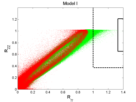
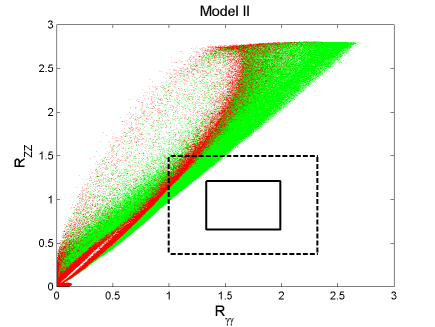
Figure 1: $R_{ZZ}$ as a function of $R_{\gamma\gamma}$ for models I and II. Green (light) points represent all points generated, red (dark) ones correspond to the existence of a panic vacuum ($D<0$). The solid (dashed) lines correspond to $1\sigma$ ($2\sigma$) experimental bounds on the rates.

rates of the light Higgs $h$ into two $Z$ bosons versus the rate of $h$ into two photons. In green (light grey) are all the points obtained in our scan, with the above constraints, both theoretical and experimental. In red (black) we show the points for which a panic vacuum occurs - meaning, points for which the value of $D$, calculated from eq. (5), is negative. It is important to consider that the density of points generated is so large that there are many green points scattered in the middle of the red ones - meaning, the areas marked red are not necessarily excluded (a consequence, of course, of the fact that we are dealing with an 8-dimensional parameter space, and these figures are only 2-dimensional). Fig. 1 clearly shows that there are regions, in the plane $R_{\gamma\gamma}$-$R_{ZZ}$, which are completely free from panic vacua. The solid and dashed lines shown in the plots correspond to conservative $1\sigma$ and $2\sigma$ intervals on the combined values for $R_{ZZ}$ and $R_{\gamma\gamma}$, $R_{ZZ}=0.93\pm 0.28$, $R_{\gamma\gamma}=1.66\pm 0.33$, which we took from ref. average , based on the LHC data before the Moriond conference cms_atlas . Notice that after the recent Moriond update on the LHC results Moriond these numbers may have changed substantially, but there isn’t yet an official combination of the ATLAS and CMS results. However, the plots we show in this communication have the advantage of being easily adapted for changing LHC experimental bounds, by simply drawing over them different black lines.

The remarkable thing is how much the current LHC data already can tell us about the nature of the 2HDM vacuum, even if no extra scalars have been found. In fact, as can be seen from Fig. 1, the panic points are distant from even the $2\sigma$ bands, which include some non-panic region as well, for model Type I. That does not occur in model Type II, in which some of the panic region is inside the $2\sigma$ region. But notice that there are many choices of parameter space values still allowed by the current data for Model II which do not lead to panic vacua. Thus, at least in these two variables, both types of models are capable of describing the current data. Nonetheless, that data does not exclude the possibility, in model type II, of our vacuum being metastable.

It has been possible to measure at the LHC - with considerable uncertainty - the production of Higgs bosons via different processes, namely gluon-gluon fusion and vector boson fusion (VBF). Analysing these processes separately gives us information about the coupling of the Higgs to both fermion (the gluon-gluon process) and gauge bosons (the VBF one). We shall use the results of the ATLAS experiment cms_atlas , which appear as $1\sigma$ and $2\sigma$ ellipses in the $R^{gg}_{\gamma\gamma}$-$R^{VBF}_{\gamma\gamma}$ plane. Our results appear in Fig. 2, for both Type I and Type II models. We observe that the experimental exclusion

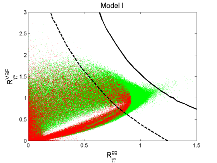
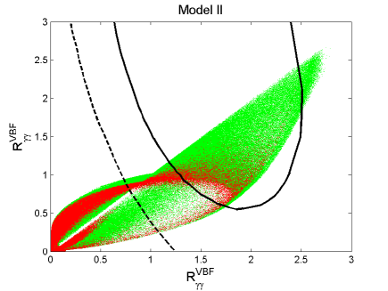
Figure 2: $R_{\gamma\gamma}$, with Higgs production via gluon-gluon fusion versus vector boson fusion production, for models I and II. Same colour codes as Fig. 1.

of points with panic vacua is not as thorough as that which happened with the previous observables. In model Type I it is not possible to exclude, at $2\sigma$, the existence of panic vacua. However, the panic vacua points which now seem allowed have been excluded in Fig. 1. For model Type II, even the $1\sigma$ bands include panic vacua solutions. We observe, nonetheless, that the ellipses contain plenty of green/light grey points as well - which means that there are many allowed choices of parameters for which panic vacua do not occur. We even see that in these variables the Type II model agrees with the data at the $1\sigma$ level, something which the Type I model cannot achieve.

The current results for a Higgs decaying to $\tau\bar{\tau}$ are compatible with the expected SM value. In fact, ATLAS measured $R_{\tau\tau}=0.7\pm 0.7$ and CMS $R_{\tau\tau}=0.72\pm 0.52$. We can see how the panic vacua points are distributed in the $\{R_{\tau\tau}\,,\,R_{\gamma\gamma}\}$ in Fig. 3.

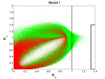
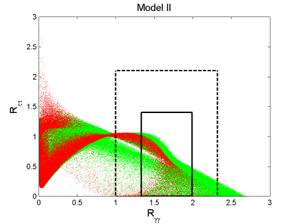
Figure 3: $R_{\tau\tau}$ as a function of $R_{\gamma\gamma}$ for models Type I and Type II. Same colour codes as Fig. 1

The $\tau\tau$ data (we represent the less restrictive bounds, those of ATLAS), tells us that panic vacua are $2\sigma$ disfavored in model Type I, and that model barely agrees, at $2\sigma$, with the LHC results in $R_{\gamma\gamma}$, agreeing at $1\sigma$ in $R_{\tau\tau}$). In model Type II, there are many panic vacua solutions not excluded by the data at $1\sigma$; but for much of Model II’s parameter space, we have agreement with the experimental results at the $1\sigma$ level, with or without panic vacua.

IV Conclusions

The rich vacuum structure of the 2HDM includes the possibility of two neutral minima being able to coexist at different depths. Thus there is the possibility that the vacuum we are currently living in is metastable, which we called the panic vacuum. It is possible to find an extremely simple criterium, the discriminant $D$ of eq. (5) being positive, which, if obeyed, guarantees that no metastability occurs. We emphasise that this situation is quite different from the SM one: there a metastable (or even unstable) vacuum may develop but only due to radiative corrections. In fact, the importance of radiative corrections to the results found here cannot be overstated, and remains an open question. We also performed an estimate of the lifetime of the false vacuum in the panic situation, and verified that it is, for the vast majority of the points scanned, much inferior to the age of the universe - as such, these panic vacua are indeed to be excluded, since “our” vacuum would have decayed long ago. Nevertheless, we see that the current LHC results already tell us a lot about the stability of the vacuum in the 2HDM. For instance, a measurement of $R_{ZZ}$ and $R_{\gamma\gamma}$ very close to 1, with sufficient precision, would exclude the possibility of panic vacua. We also saw that the values of the parameters of the potential which produce panic vacua do not correspond to uninteresting regions of the model - rather, they predict observables which are not absurd and indeed may fall into the current experimental bounds. This, by itself, indicates the need to take seriously this possibility of vacuum instability in the 2HDM.

- (1) T. D. Lee, Phys. Rev. D 8 (1973) 1226.
- (2) G. C. Branco, P. M. Ferreira, L. Lavoura, M. N. Rebelo, M. Sher and J. P. Silva, Phys. Rept. 516, 1 (2012) [arXiv:1106.0034 [hep-ph]].
- (3) G. Aad et al. [ATLAS Collaboration], Phys. Lett. B 716, 1 (2012) [arXiv:1207.7214 [hep-ex]].
- (4) S. Chatrchyan et al. [CMS Collaboration], Phys. Lett. B 716, 30 (2012) [arXiv:1207.7235 [hep-ex]].
- (5) C. -Y. Chen and S. Dawson, arXiv:1301.0309 [hep-ph].
- (6) G. Belanger, B. Dumont, U. Ellwanger, J. F. Gunion and S. Kraml, arXiv:1212.5244 [hep-ph].
- (7) S. Chang, S. K. Kang, J. -P. Lee, K. Y. Lee, S. C. Park and J. Song, with mass around 125 GeV,” arXiv:1210.3439 [hep-ph].
- (8) P. M. Ferreira, R. Santos, M. Sher and J. P. Silva, Phys. Rev. D 85, 077703 (2012) [arXiv:1112.3277 [hep-ph]].
- (9) A. Barroso, P. M. Ferreira, I. P. Ivanov and R. Santos, arXiv:1303.5098 [hep-ph].
- (10) P. M. Ferreira, R. Santos and A. Barroso, Phys. Lett. B 603 (2004) 219 [Erratum-ibid. B 629 (2005) 114] [arXiv:hep-ph/0406231].
- (11) A. Barroso, P. M. Ferreira and R. Santos, Phys. Lett. B 632 (2006) 684 [arXiv:hep-ph/0507224].
- (12) A. Barroso, P. M. Ferreira and R. Santos, Phys. Lett. B 652 (2007) 181 [arXiv:hep-ph/0702098].
- (13) I. P. Ivanov, Phys. Rev. D 75 (2007) 035001 [Erratum-ibid. D 76 (2007) 039902] [arXiv:hep-ph/0609018].
- (14) I. P. Ivanov, Phys. Rev. D 77 (2008) 015017 [arXiv:0710.3490 [hep-ph]].
- (15) A. Barroso, P. M. Ferreira, I. P. Ivanov, R. Santos and J. P. Silva, arXiv:1211.6119 [hep-ph].
- (16) R. D. Peccei and H. R. Quinn, Phys. Rev. Lett. 38 (1977) 1440.
- (17) S. L. Glashow and S. Weinberg, Phys. Rev. D 15 (1977) 1958.
- (18) E. A. Paschos, Phys. Rev. D 15 (1977) 1966.
- (19) I. P. Ivanov, Phys. Rev. E 79, 021116 (2009).
- (20) S. Kanemura, T. Kubota and E. Takasugi, Phys. Lett. B 313 (1993) 155 [arXiv:hep-ph/9303263].
- (21) A. G. Akeroyd, A. Arhrib and E. -M. Naimi, Phys. Lett. B 490, 119 (2000) [hep-ph/0006035].
- (22) M.E. Peskin and T. Takeuchi, Phys. Rev. D 46, 381 (1992).
- (23) The ALEPH, CDF, D0, DELPHI, L3, OPAL, SLD Collaborations, the LEP Electroweak Working Group, the Tevatron Electroweak Working Group, and the SLD electroweak and heavy flavour Groups, arXiv:1012.2367 [hep-ex].
- (24) M. Baak, M. Goebel, J. Haller, A. Hoecker, D. Ludwig, K. Moenig, M. Schott and J. Stelzer, Eur. Phys. J. C 72, 2003 (2012) [arXiv:1107.0975 [hep-ph]].
- (25) M. Baak, M. Goebel, J. Haller, A. Hoecker, D. Kennedy, R. Kogler, K. Moenig, M. Schott and J. Stelzer, arXiv:1209.2716 [hep-ph].
- (26) T. Hermann, M. Misiak and M. Steinhauser, Next-to-Next-to-Leading Order in QCD,” JHEP 1211 (2012) 036 [arXiv:1208.2788 [hep-ph]].
- (27) F. Mahmoudi, talk given at Prospects For Charged Higgs Discovery At Colliders (CHARGED 2012), 8-11 October, Uppsala, Sweden.
- (28) For recent results, see G. Aad et al. [ATLAS Collaboration], Phys. Lett. B 716, 1 (2012) [arXiv:1207.7214 [hep-ex]]. S. Chatrchyan et al. [CMS Collaboration], Phys. Lett. B 716, 30 (2012) [arXiv:1207.7235 [hep-ex]].
- (29) A. Arbey, M. Battaglia, A. Djouadi and F. Mahmoudi, arXiv:1211.4004 [hep-ph].
- (30) The ATLAS collaboration, ATLAS-CONF-2013-012, ATLAS-CONF-2013-013, ATLAS-CONF-2013-030, ATLAS-CONF-2013-034. The CMS collaboration, CMS notes CMS-PAS-HIG-13-001, CMS-PAS-HIG-13-002, CMS-PAS-HIG-13-003 and CMS-PAS-HIG-13-003.