A Nested Dissection Approach to Modeling Transport in Nanodevices: Algorithms and Applications

Abstract

Modeling nanoscale devices quantum mechanically is a computationally challenging problem where new methods to solve the underlying equations are in a dire need. In this paper, we present an approach to calculate the charge density in nanoscale devices, within the context of the non equilibrium Green’s function approach. Our approach exploits recent advances in using an established graph partitioning approach. The developed method has the capability to handle open boundary conditions that are represented by full self energy matrices required for realistic modeling of nanoscale devices. Our method to calculate the electron density has a reduced complexity compared to the established recursive Green’s function approach. As an example, we apply our algorithm to a quantum well superlattice and a carbon nanotube, which are represented by a continuum and tight binding Hamiltonian respectively, and demonstrate significant speed up over the recursive method.

keywords: nanodevice, numerical simulation, device modeling, quantum transport, superlattice, nanomaterials, graphene, Green’s functions, nanotechnology, nanotransistor, tunneling, design

1 Introduction

With the advent of smaller nanoelectronic devices, where quantum mechanics is central to the device operation, and new nanomaterials, such as nanotubes, graphene, and nanowires, quantum mechanical simulations have become a necessity. The non-equilibrium Green’s function (NEGF) method [1, 2, 3] has emerged as a powerful modeling approach for these nanodevices and nanomaterials. The NEGF method is based on the self-consistent coupling of Schrödinger and Poisson equations and is designed to capture electron scattering effects with phonons.

A typical NEGF-based simulation solves three Green’s function equations,

$$\begin{cases}\mathbf{A}\left(E\right)\mathbf{G}^{r}\left(E\right)&=\;\mathbf{I}\\ \mathbf{A}\left(E\right)\mathbf{G}^{<}\left(E\right)&=\;\boldsymbol{\Sigma}^{<}\left(\mathbf{G}^{r}\left(E\right)\right)^{\dagger}\\ \mathbf{A}\left(E\right)\mathbf{G}^{>}\left(E\right)&=\;\boldsymbol{\Sigma}^{>}\left(\mathbf{G}^{r}\left(E\right)\right)^{\dagger}\end{cases}$$ (1)

where the sparse matrix $\mathbf{A}$ is defined by

$$\mathbf{A}=E\mathbf{I}-\mathbf{H}-\boldsymbol{\Sigma}^{r}_{L}-\boldsymbol{\Sigma}^{r}_{R}-\boldsymbol{\Sigma}^{r}_{Phonon}$$ (2)

$\mathbf{G}^{r}(E)$ is called the retarded Green’s function, describing local density of states and the propagation of electrons injected in the device, and $\left(\mathbf{G}^{r}(E)\right)^{\dagger}$ its Hermitian conjugate. $\mathbf{G}^{<}(E)$, the lesser Green’s function, represents the electron correlation function for energy level $E$; the diagonal elements of $\mathbf{G}^{<}(E)$ represent the electron density per unit energy. $\mathbf{G}^{>}(E)$, the greater Green’s function, represents the hole correlation function for energy level $E$, which is proportional to the density of unoccupied states. $\mathbf{I}$ is the identity matrix and $\mathbf{H}$ the system Hamiltonian. $\boldsymbol{\Sigma}^{r}_{L}$ and $\boldsymbol{\Sigma}^{r}_{R}$ represent the self-energies due to left and right contact coupling and $\boldsymbol{\Sigma}^{r}_{Phonon}$ corresponds to the self-energy governing electron-phonon scattering. The matrix $\boldsymbol{\Sigma}^{<}$ corresponds to the lesser self-energy and the matrix $\boldsymbol{\Sigma}^{>}$ to the greater self-energy. The Green functions are then incorporated in the coupling between the Schrödinger and Poisson equations – see [1] for further details. The self-consistent solution of the Schrödinger and Poisson equations requires to solve (1) many times until consistency is achieved. It is well appreciated that the computationally intensive part of this calculation is solving (1) for the diagonal element of $\mathbf{G}^{<}$ (electron density) and $\mathbf{G}^{>}$ at all energies $E$. The objective of this paper is to present a new algorithm for accelerating the solution of (1).

The recursive Green’s function method (RGF) [7, 6, 8, 10, 20] is an effective method, often used in practice, to compute $\mathbf{G}^{r}$, $\mathbf{G}^{<}$, and $\mathbf{G}^{>}$. For elongated devices, this approach remains the most efficient. Recently, the Hierarchical Schur Complement (HSC) method [14, 15] and the Fast Inverse using Nested Dissection (FIND) method [11, 12] exploit the nested dissection method [5] to exhibit a significant speedup. The key ideas behind these two algorithms are to partition the whole matrix $\mathbf{A}$ into blocks for an efficient block LU-factorization. This factorization is then re-used to fill in all diagonal blocks of the Green’s function and some off-diagonal blocks in a specific order. These two algorithms are more efficient than RGF and have reduced the operation count down to a multiple of the cost for a block LU-factorization of a sparse matrix. Approximate methods, that are efficient in the ballistic limit, exist also. For example, the contact block reduction [16, 17] accelerates the computation by using a limited number of modes to represent the matrices. The focus of this paper is to develop an exact method that works in the presence of scattering.

For calculating the lesser Green’s function $\mathbf{G}^{<}$, advanced algorithms for an arbitrary sparse matrix are still in their infancy. The RGF method remains an effective method, especially for elongated devices. The extension of FIND [12] for $\mathbf{G}^{<}$ yields a reduced asymptotic complexity but the constant in front of the asymptotic term hinders the reduction in runtime. Li et al. [13] have recently proposed a modification of FIND for a significant speedup but their partitioning of the matrix $\mathbf{A}$ requires some pre-processing. The contribution of this paper is to present an extension of the HSC method for calculating diagonal blocks for $\mathbf{G}^{<}$ with partitions from existing graph partitioning libraries (like, for example, the package METIS [9]).

The rest of the paper is organized as follows. Section 2 will review exact methods and discuss differences between previous algorithms and the proposed approach. Section 3 will give a mathematical description of the new algorithm. Finally, Section 4 describes numerical experiments to highlight its efficiency. The discussion and analysis in this paper will focus on two-dimensional problems, while three-dimensional problems will be illustrated in a future publication.

2 Review of Eexact Methods

Consider a device that can be topologically broken down into layers as shown in Figure 1. For an effective mass Hamiltonian, the blue dots represent grid points of the discretized Green’s function equation, while, in the case of a tight binding Hamiltonian, the blue dots represent orbitals on an atom.

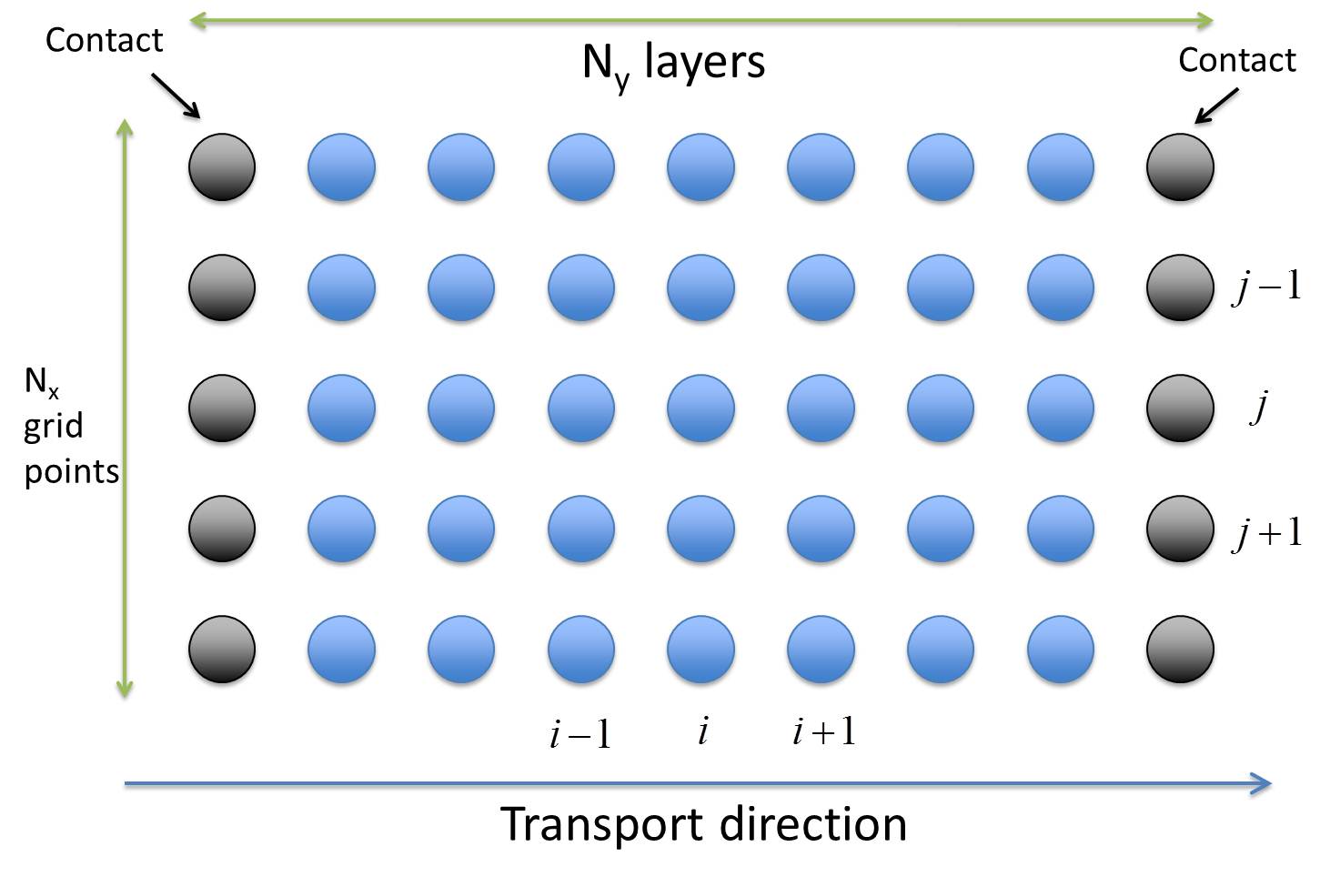
Figure 1: Nano-device partitioned into $N_{y}$ layers. Each layer contains $N_{x}$ grid points.

When a five-point stencil is used for discretization, the resulting Hamiltonian is a symmetric block tri-diagonal matrix as shown in Figure 2, where each diagonal block represents the Hamiltonian of a layer in Figure 1. The $i$-th diagonal block of the Hamiltonian represents the coupling between grid points / atoms in a layer. The off-diagonal blocks to its left and right represents coupling to between layers $i$ and $i-1$ and $i+1$ respectively. Both the diagonal and off-diagonal blocks of the Hamiltonian are sparse in many examples where either an effective mass or a tight-binding Hamiltonian represents the dynamics — examples of such device include silicon nanowires, nanotubes, and graphene.

The left and right coupling contacts (indicated in Figure 1) are two semi-infinite leads connected with the device and infinite matrices represent their Hamiltonians. Their respective effect can be folded into layer 1 and layer $N_{y}$, resulting in dense blocks for the first and the $N_{y}$-th diagonal blocks of the self-energy matrices $\boldsymbol{\Sigma}^{r}_{L}$ and $\boldsymbol{\Sigma}^{r}_{R}$. The resulting matrix structure of the matrix $\mathbf{A}$, defined in (2), is shown in Figure 2. Note that the self-energy matrix $\boldsymbol{\Sigma}^{r}_{Phonon}$ is set to be diagonal at each interior grid point, which may arise due to electron-phonon interaction or any other interaction. Relaxing the requirement of diagonal $\boldsymbol{\Sigma}^{r}_{Phonon}$ to include more realistic models of scattering and solving equations (1) remains a challenge.

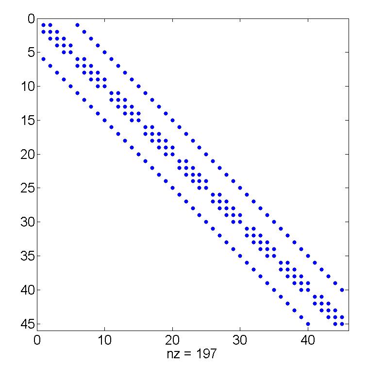
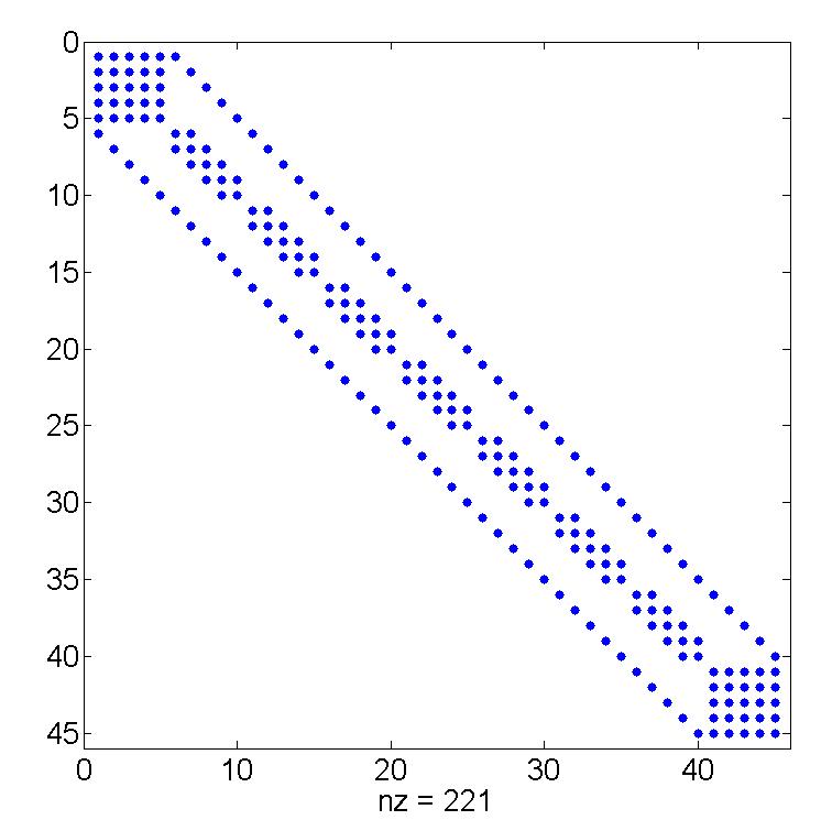
Figure 2: $\mathbf{H}$ (left) and $\mathbf{A}$ (right) matrix shape, non-zero entries are highlighted.

The most common approach to compute blocks of $\mathbf{G}^{r}$ and $\mathbf{G}^{<}$ is the recursive Green’s function method [21, 1]. RGF is an algorithm composed of two passes to compute $\mathbf{G}^{r}$ and two passes to compute $\mathbf{G}^{<}$. In both cases, the passes are interpreted as follows:

1. the first pass marches one layer at a time from left to right along the $y$-direction and, recursively, folds the effect of left layers into the current layer;

2. the second pass marches one layer at a time from right to left along the $y$-direction and, recursively, extracts the diagonal blocks and the nearest neighbor off-diagonal blocks for the final result.

Numerically, it is essential to notice that the RGF method exploits the matrix sparsity of only at the block level, which means that it separates the whole problem into sub-problems of full matrix operations. The complexity of this method is, at most, $10N_{x}^{3}N_{y}$ (when $N_{x}\leq N_{y}$).

To compute block entries of $\mathbf{G}^{r}$, two recent advances, namely FIND [11, 12] and HSC [14, 15], utilize the nested dissection method [5] to exhibit a significant speedup. These methods explicitly exploit the sparsity of $\mathbf{A}$ via a sparse block LU-factorization of the whole matrix and re-use this factorization to fill in all diagonal blocks of the Green’s function and some off-diagonal blocks in a specific order. FIND and HSC have a strong mathematical component and their physical interpretation is less obvious. The main difference between RGF and these methods is the replacement of layers of grid points organized along a specific direction with arbitrarily-shaped clusters of grid points organized in a binary tree. Such choice allows to fold and to extract in any physical direction when following the vertical hierarchy of the binary tree. Further details about FIND and HSC can be found in their respective references. Table 1 summarizes the complexity of these three state-of-the-art algorithms when computing entries in $\mathbf{G}^{r}$.

Algorithm	Complexity when $N_{x}=N_{y}$	Complexity when $N_{x}<N_{y}$
RGF [21]	$\mathcal{O}\left(N_{x}^{4}\right)$	$\leq 10N_{x}^{3}N_{y}$
FIND [11, 18]	$\mathcal{O}\left(N_{x}^{3}\right)$	$\leq 143N_{x}^{2}N_{y}$
HSC [14, 18]	$\mathcal{O}\left(N_{x}^{3}\right)$	$\leq 87N_{x}^{2}N_{y}$

Table 1: Complexity of algorithms to compute diagonal blocks of $\mathbf{G}^{r}$.

Even though FIND [11] and HSC [14] have two distinct mathematical motivations, their runtime complexities exhibit the same dominating term. But the constants multiplying these asymptotic terms differ greatly. The runtime for FIND [11] contains a large constant due to the usage of thick boundaries between the clusters of grid points (or width-2 separators—a width-2 separator is a boundary between clusters that has a thickness of 2 grid points or 2 atoms). In addition, generating these clusters with thick boundaries is not compatible with most existing partitioning libraries. On the other hand, the HSC method use thin boundaries between clusters with a thickness of one grid point (or width-1 separators) and can directly exploit partitions from existing partitioning libraries. As a result, to compute diagonal blocks for $\mathbf{G}^{r}$, the HSC method [14, p. 758] is more efficient than FIND [11].

To compute diagonal entries for $\mathbf{G}^{<}$, only the RGF [1] and FIND [12] methods have been extended. Table 2 displays the runtime complexity for computing diagonal blocks of $\mathbf{G}^{<}$.

Algorithm	Complexity when $N_{x}=N_{y}$	Complexity when $N_{x}<N_{y}$
RGF [21]	$\leq 4N_{x}^{4}$	$\mathcal{O}\left(N_{x}^{3}N_{y}\right)$
FIND [12]	$\leq 457N_{x}^{3}$	$\mathcal{O}\left(N_{x}^{2}N_{y}\right)$

Table 2: Complexity of algorithms to compute diagonal blocks of $\mathbf{G}^{<}$.

The extension of FIND [12] for $\mathbf{G}^{<}$ still use thick boundaries that result in a large constant for the runtime and that are incompatible with existing partitioning libraries. Recently, Li et al. [13] have proposed an extension of FIND [11, 12] that enables thin boundaries (width-1 separators). This new algorithm yields a significant speedup over earlier versions of FIND [11, 12]. The mathematical motivation remains different from HSC. The clustering part needs to identify peripheral sets, an information that is not provided directly by most partitioning libraries.

The contribution of this paper is to present an extension of the HSC method [14] for calculating the diagonal blocks for $\mathbf{G}^{<}$. This extension uses thin boundaries (or width-1 separators) and is compatible with existing partitioning libraries — namely, the extension is combined with the graph partitioning package METIS [9]. The same extension computes efficiently diagonal blocks for $\mathbf{G}^{>}$ in a separate step. For the sake of conciseness, the rest of the paper is focused only on computing $\mathbf{G}^{<}$.

3 Mathematical Description of the Algorithm

In this section, a detailed mathematical description for the extension of HSC to compute blocks of $\mathbf{G}^{<}$ is given. The key ingredients are:

1. an efficient sparse block $\mathbf{LDL}^{T}$-factorization of $\mathbf{A}$. The block sparse factorization will gather grid points into arbitrarily-shaped clusters (instead of layers, like in RGF). Such choice allows to fold and to extract in any physical direction when eliminating entries in $\mathbf{A}$. The factorization yields formulas to calculate the diagonal blocks and off-diagonal blocks for $\mathbf{G}^{r}$ and $\mathbf{G}^{<}$. Exploiting the resulting algebraic relations results in an algorithm with a cost significantly smaller than the full inversion of matrix $\mathbf{A}$.

2. an appropriate order of operations. The cost of a matrix multiplication $\mathbf{BCD}$ depends on the order of operations. When $\mathbf{B}$ is $m\times p$, $\mathbf{C}$ is $p\times k$, and $\mathbf{D}$ is $k\times n$, $\left(\mathbf{BC}\right)\mathbf{D}$ costs $2mk(n+p)$ operations and $\mathbf{B}\left(\mathbf{CD}\right)$ costs $2np(m+k)$. The order of operations can have a large effect when multiplying series of matrices together (which is the case for computing entries of $\mathbf{G}^{r}$ and $\mathbf{G}^{<}$). Furthermore, when working with sparse matrices, one order of operations may preserve sparsity, while another may not.

First, a simple description with three clusters is given. Then the approach is extended to an arbitrary number of levels and a multilevel binary tree.

3.1 Description for a simple case

The basic idea is to partition the nano-device into three disjoint regions (L, R, S) — see Figure 3

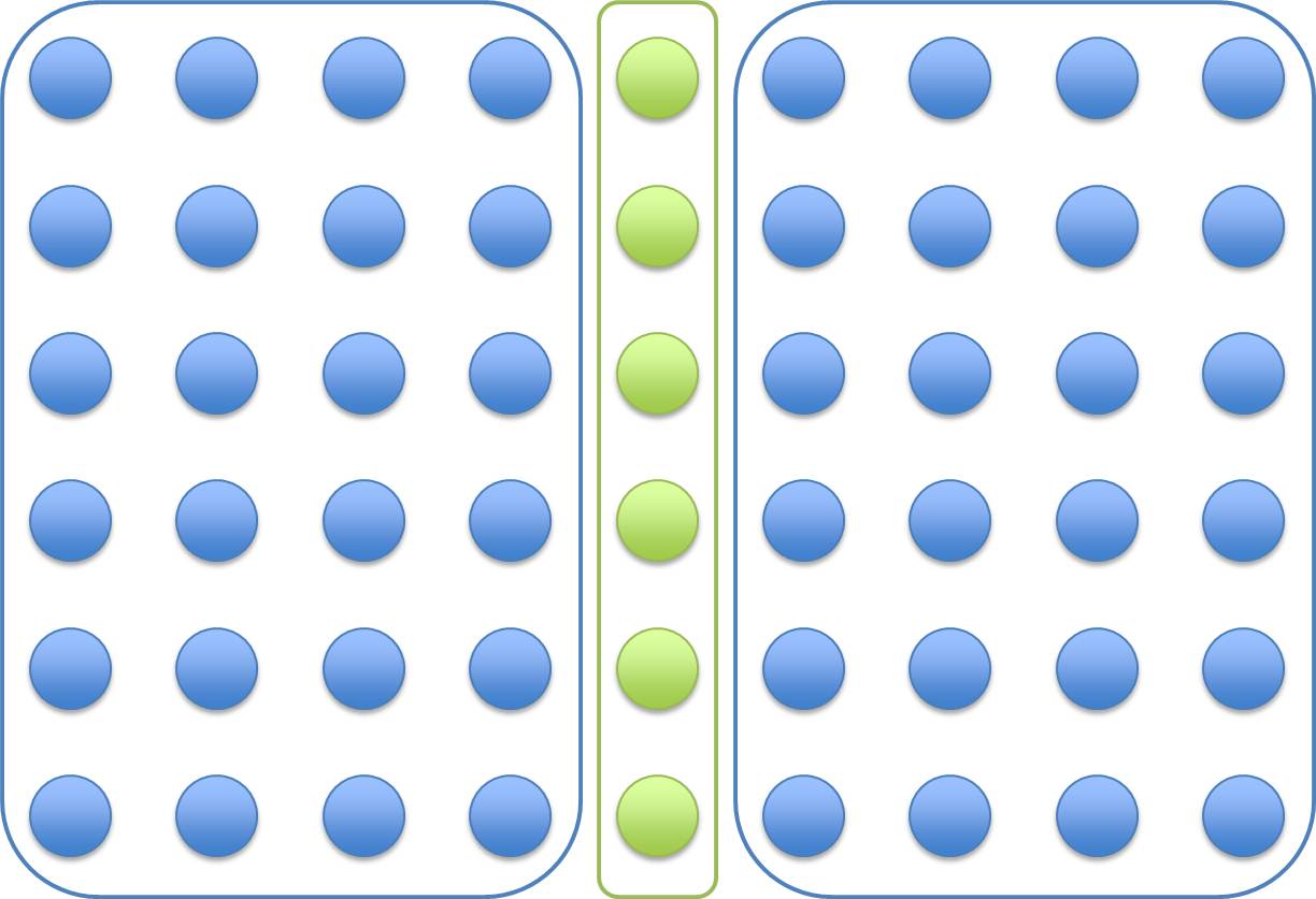
Figure 3: Nanodevice partitioned into two subregions (L, R) and a separator S (L stands for Left and R for Right).

Such a partition is easily obtained via the nested dissection, introduced by George [5]. Nested dissection divides the system into two disconnected sets and an interface, called the separator S. With this partition, the matrix $\mathbf{A}$ can be written as

$$\mathbf{A}=\left[\begin{array}[]{ccc}\mathbf{A}_{LL}&\mathbf{0}&\mathbf{A}_{LS}\\ \mathbf{0}&\mathbf{A}_{RR}&\mathbf{A}_{RS}\\ \mathbf{A}_{LS}^{T}&\mathbf{A}_{RS}^{T}&\mathbf{A}_{SS}\end{array}\right]$$

Note that matrix $\mathbf{A}$ is typically complex symmetric. The block $\mathbf{LDL}^{T}$-factorization of $\mathbf{A}$ is

$$\mathbf{A}=\left[\begin{array}[]{ccc}\mathbf{I}&\mathbf{0}&\mathbf{0}\\ \mathbf{0}&\mathbf{I}&\mathbf{0}\\ \mathbf{A}_{LS}^{T}\mathbf{A}_{LL}^{-1}&\mathbf{A}_{RS}^{T}\mathbf{A}_{RR}^{-1}&\mathbf{I}\end{array}\right]\left[\begin{array}[]{ccc}\mathbf{A}_{LL}&\mathbf{0}&\mathbf{0}\\ \mathbf{0}&\mathbf{A}_{RR}&\mathbf{0}\\ \mathbf{0}&\mathbf{0}&\widehat{\mathbf{A}}_{SS}\end{array}\right]\left[\begin{array}[]{ccc}\mathbf{I}&\mathbf{0}&\mathbf{A}_{LL}^{-1}\mathbf{A}_{LS}\\ \mathbf{0}&\mathbf{I}&\mathbf{A}_{RR}^{-1}\mathbf{A}_{RS}\\ \mathbf{0}&\mathbf{0}&\mathbf{I}\end{array}\right]$$

where $\widehat{\mathbf{A}}_{SS}$ is the Schur complement,

$$\widehat{\mathbf{A}}_{SS}=\mathbf{A}_{SS}-\mathbf{A}_{LS}^{T}\mathbf{A}_{LL}^{-1}\mathbf{A}_{LS}-\mathbf{A}_{RS}^{T}\mathbf{A}_{RR}^{-1}\mathbf{A}_{RS}.$$

The matrix $\mathbf{G}^{r}$ satisfies the relation

$$\mathbf{G}^{r}=\left(\mathbf{I}-\mathbf{L}^{T}\right)\mathbf{G}^{r}+\mathbf{D}^{-1}\mathbf{L}^{-1}\quad\mbox{with}\quad\mathbf{A}=\mathbf{LD}\mathbf{L}^{T}$$ (3)

(described in Takahashi et al. [22] and Erisman and Tinney [4]). The block notation yields

$$\mathbf{G}^{r}=-\left[\begin{array}[]{ccc}\mathbf{A}_{LL}^{-1}\mathbf{A}_{LS}\mathbf{G}_{SL}^{r}&\mathbf{A}_{LL}^{-1}\mathbf{A}_{LS}\mathbf{G}_{SR}^{r}&\mathbf{A}_{LL}^{-1}\mathbf{A}_{LS}\mathbf{G}_{SS}^{r}\\ \mathbf{A}_{RR}^{-1}\mathbf{A}_{RS}\mathbf{G}_{SL}^{r}&\mathbf{A}_{RR}^{-1}\mathbf{A}_{RS}\mathbf{G}_{SR}^{r}&\mathbf{A}_{RR}^{-1}\mathbf{A}_{RS}\mathbf{G}_{SS}^{r}\\ \mathbf{0}&\mathbf{0}&\mathbf{\mathbf{0}}\end{array}\right]\\ +\left[\begin{array}[]{ccc}\mathbf{A}_{LL}^{-1}&\mathbf{0}&\mathbf{0}\\ \mathbf{0}&\mathbf{A}_{RR}^{-1}&\mathbf{0}\\ \mathbf{0}&\mathbf{0}&\widehat{\mathbf{A}}_{SS}^{-1}\end{array}\right]\left[\begin{array}[]{ccc}\mathbf{I}&\mathbf{0}&\mathbf{0}\\ \mathbf{0}&\mathbf{I}&\mathbf{0}\\ -\mathbf{A}_{LS}^{T}\mathbf{A}_{LL}^{-1}&-\mathbf{A}_{RS}^{T}\mathbf{A}_{RR}^{-1}&\mathbf{I}\end{array}\right].$$

This equation indicates

$$\mathbf{G}_{SS}^{r} =\left(\widehat{\mathbf{A}}_{SS}\right)^{-1},$$

$$\mathbf{G}_{LS}^{r} =-\mathbf{A}_{LL}^{-1}\mathbf{A}_{LS}\mathbf{G}_{SS}^{r},$$

$$\mathbf{G}_{RS}^{r} =-\mathbf{A}_{RR}^{-1}\mathbf{A}_{RS}\mathbf{G}_{SS}^{r}.$$

The diagonal blocks $\mathbf{G}_{LL}^{r}$ and $\mathbf{G}_{RR}^{r}$, for the regions L and R, respectively, are computed independently of each other,

$$\mathbf{G}_{LL}^{r} =\mathbf{A}_{LL}^{-1}-\mathbf{A}_{LL}^{-1}\mathbf{A}_{LS}\left(\mathbf{G}_{LS}^{r}\right)^{T}=\mathbf{A}_{LL}^{-1}+\mathbf{A}_{LL}^{-1}\mathbf{A}_{LS}\mathbf{G}_{SS}^{r}\mathbf{A}_{LS}^{T}\mathbf{A}_{LL}^{-1}$$

$$\mathbf{G}_{RR}^{r} =\mathbf{A}_{RR}^{-1}-\mathbf{A}_{RR}^{-1}\mathbf{A}_{RS}\left(\mathbf{G}_{RS}^{r}\right)^{T}=\mathbf{A}_{RR}^{-1}+\mathbf{A}_{RR}^{-1}\mathbf{A}_{RS}\mathbf{G}_{SS}^{r}\mathbf{A}_{RS}^{T}\mathbf{A}_{RR}^{-1}$$

(where the symmetry of $\mathbf{G}^{r}$ has been exploited). For this simple case, the resulting algorithm matches exactly the HSC method [14].

For calculating entries in the correlation matrix $\mathbf{G}^{<}$, Petersen et al. [18] generalized Takahashi’s method by writing

$$\mathbf{L}^{T}\mathbf{G}^{<}\left(\mathbf{L}^{T}\right)^{\dagger}=\mathbf{D}^{-1}\mathbf{L}^{-1}\boldsymbol{\Sigma}^{<}\mathbf{L}^{-\dagger}\mathbf{D}^{-\dagger}.$$ (4)

Recurrence formulas are described in [18]. Our approach utilizes a variant of (4), namely

$$\mathbf{G}^{<}=\left(\mathbf{I}-\mathbf{L}^{T}\right)\mathbf{G}^{<}+\mathbf{D}^{-1}\mathbf{L}^{-1}\boldsymbol{\Sigma}^{<}\left(\mathbf{G}^{r}\right)^{\dagger},$$ (5)

and exploits the symmetry of $\mathbf{G}^{r}$ and the skew-Hermitian property of $\boldsymbol{\Sigma}^{<}$ and $\mathbf{G}^{<}$,

$$\left(\mathbf{G}^{<}\right)^{\dagger}=-\mathbf{G}^{<}\quad\mbox{ and }\quad\left(\boldsymbol{\Sigma}^{<}\right)^{\dagger}=-\boldsymbol{\Sigma}^{<}.$$ (6)

The block $\mathbf{LDL}^{T}$-factorization of $\mathbf{A}$ yields

$$\mathbf{G}^{<}=-\left[\begin{array}[]{ccc}\mathbf{A}_{LL}^{-1}\mathbf{A}_{LS}\mathbf{G}_{SL}^{<}&\mathbf{A}_{LL}^{-1}\mathbf{A}_{LS}\mathbf{G}_{SR}^{<}&\mathbf{A}_{LL}^{-1}\mathbf{A}_{LS}\mathbf{G}_{SS}^{<}\\ \mathbf{A}_{RR}^{-1}\mathbf{A}_{RS}\mathbf{G}_{SL}^{<}&\mathbf{A}_{RR}^{-1}\mathbf{A}_{RS}\mathbf{G}_{SR}^{<}&\mathbf{A}_{RR}^{-1}\mathbf{A}_{RS}\mathbf{G}_{SS}^{<}\\ \mathbf{0}&\mathbf{0}&\mathbf{\mathbf{0}}\end{array}\right]\\ +\left[\begin{array}[]{ccc}\mathbf{A}_{LL}^{-1}&\mathbf{0}&\mathbf{0}\\ \mathbf{0}&\mathbf{A}_{RR}^{-1}&\mathbf{0}\\ \mathbf{0}&\mathbf{0}&\left(\widehat{\mathbf{A}}_{SS}\right)^{-1}\end{array}\right]\left[\begin{array}[]{ccc}\mathbf{I}&\mathbf{0}&\mathbf{0}\\ \mathbf{0}&\mathbf{I}&\mathbf{0}\\ -\mathbf{A}_{LS}^{T}\mathbf{A}_{LL}^{-1}&-\mathbf{A}_{RS}^{T}\mathbf{A}_{RR}^{-1}&\mathbf{I}\end{array}\right]\boldsymbol{\Sigma}^{<}\left(\mathbf{G}^{r}\right)^{\dagger}.$$

Parts of $\mathbf{G}^{r}$ are computed with the previous algorithm, namely, $\mathbf{G}_{LL}^{r}$, $\mathbf{G}_{RR}^{r}$, $\mathbf{G}_{SS}^{r}$, $\mathbf{G}_{RS}^{r}$, and $\mathbf{G}_{LS}^{r}$. By assumption, $\boldsymbol{\Sigma}^{<}$ is a block-diagonal skew-Hermitian matrix with purely imaginary entries. The partial matrix multiplication gives

$$\left[\begin{array}[]{ccc}\mathbf{I}&\mathbf{0}&\mathbf{0}\\ \mathbf{0}&\mathbf{I}&\mathbf{0}\\ -\mathbf{A}_{LS}^{T}\mathbf{A}_{LL}^{-1}&-\mathbf{A}_{RS}^{T}\mathbf{A}_{RR}^{-1}&\mathbf{I}\end{array}\right]\boldsymbol{\Sigma}^{<}\left(\mathbf{G}^{r}\right)^{\dagger}=\\ \left[\begin{array}[]{ccc}\boldsymbol{\Sigma}_{LL}^{<}\left(\mathbf{G}_{LL}^{r}\right)^{\dagger}&\mathbf{*}&\boldsymbol{\Sigma}_{LL}^{<}\left(\mathbf{G}_{SL}^{r}\right)^{\dagger}\\ &\boldsymbol{\Sigma}_{RR}^{<}\left(\mathbf{G}_{RR}^{r}\right)^{\dagger}&\boldsymbol{\Sigma}_{RR}^{<}\left(\mathbf{G}_{RS}^{r}\right)^{\dagger}\\ \mathbf{*}&\mathbf{*}&\boldsymbol{\Sigma}_{SS}^{<}\left(\mathbf{G}_{SS}^{r}\right)^{\dagger}-\mathbf{A}_{LS}^{T}\mathbf{A}_{LL}^{-1}\boldsymbol{\Sigma}_{LL}^{<}\left(\mathbf{G}_{SL}^{r}\right)^{\dagger}-\mathbf{A}_{RS}^{T}\mathbf{A}_{RR}^{-1}\boldsymbol{\Sigma}_{RR}^{<}\left(\mathbf{G}_{SR}^{r}\right)^{\dagger}\end{array}\right]$$

(where the starred blocks are not computed). This relation indicates

$$\mathbf{G}_{SS}^{<} =\mathbf{G}_{SS}^{r}\left(\boldsymbol{\Sigma}_{SS}^{<}\left(\mathbf{G}_{SS}^{r}\right)^{\dagger}-\mathbf{A}_{LS}^{T}\mathbf{A}_{LL}^{-1}\boldsymbol{\Sigma}_{LL}^{<}\left(\mathbf{G}_{SL}^{r}\right)^{\dagger}-\mathbf{A}_{RS}^{T}\mathbf{A}_{RR}^{-1}\boldsymbol{\Sigma}_{RR}^{<}\left(\mathbf{G}_{SR}^{r}\right)^{\dagger}\right),$$

$$\mathbf{G}_{LS}^{<} =-\mathbf{A}_{LL}^{-1}\mathbf{A}_{LS}\mathbf{G}_{SS}^{<}+\mathbf{A}_{LL}^{-1}\boldsymbol{\Sigma}_{LL}^{<}\left(\mathbf{G}_{SL}^{r}\right)^{\dagger},$$

$$\mathbf{G}_{RS}^{<} =-\mathbf{A}_{RR}^{-1}\mathbf{A}_{RS}\mathbf{G}_{SS}^{<}+\mathbf{A}_{RR}^{-1}\boldsymbol{\Sigma}_{RR}^{<}\left(\mathbf{G}_{SR}^{r}\right)^{\dagger}.$$

Finally, the diagonal blocks $\mathbf{G}_{LL}^{<}$ and $\mathbf{G}_{RR}^{<}$, for the regions $L$ and $R$, respectively, are computed independently of each other,

$$\mathbf{G}_{LL}^{<} =\mathbf{A}_{LL}^{-1}\boldsymbol{\Sigma}_{LL}^{<}\left(\mathbf{G}_{LL}^{r}\right)^{\dagger}-\mathbf{A}_{LL}^{-1}\mathbf{A}_{LS}\left(\mathbf{G}_{LS}^{<}\right)^{\dagger}$$

$$\mathbf{G}_{RR}^{<} =\mathbf{A}_{RR}^{-1}\boldsymbol{\Sigma}_{RR}^{<}\left(\mathbf{G}_{RR}^{r}\right)^{\dagger}-\mathbf{A}_{RR}^{-1}\mathbf{A}_{RS}\left(\mathbf{G}_{RS}^{<}\right)^{\dagger}$$

(where the skew-Hermitian property of $\mathbf{G}^{<}$ has been exploited).

This derivation for calculating the correlation matrix $\mathbf{G}^{<}$ differs from the FIND method [12, 13] in several aspects. It uses thin boundaries obtained directly from the nested dissection. This extension requires one sparse factorization and one back-substitution, while FIND utilizes only sparse factorizations but applied many times with different orderings. The order of operations to obtain the diagonal blocks of $\mathbf{G}^{<}$ is also different from the recurrence in Petersen et al. [18], which uses the sequence

$$\boldsymbol{\Sigma}^{<}\rightarrow\mathbf{L}^{-1}\boldsymbol{\Sigma}^{<}\left(\mathbf{L}^{-1}\right)^{\dagger}\rightarrow\mathbf{D}^{-1}\mathbf{L}^{-1}\boldsymbol{\Sigma}^{<}\left(\mathbf{L}^{-1}\right)^{\dagger}\left(\mathbf{D}^{-1}\right)^{\dagger}\\ \rightarrow\mathbf{L}^{-T}\mathbf{D}^{-1}\mathbf{L}^{-1}\boldsymbol{\Sigma}^{<}\left(\mathbf{L}^{-1}\right)^{\dagger}\left(\mathbf{D}^{-1}\right)^{\dagger}\left(\mathbf{L}^{-T}\right)^{\dagger},$$

while our HSC extension uses

$$\boldsymbol{\Sigma}^{<}\rightarrow\boldsymbol{\Sigma}^{<}\left(\mathbf{G}^{r}\right)^{\dagger}\rightarrow\mathbf{L}^{-1}\boldsymbol{\Sigma}^{<}\left(\mathbf{G}^{r}\right)^{\dagger}\rightarrow\mathbf{D}^{-1}\mathbf{L}^{-1}\boldsymbol{\Sigma}^{<}\left(\mathbf{G}^{r}\right)^{\dagger}\rightarrow\mathbf{L}^{-T}\mathbf{D}^{-1}\mathbf{L}^{-1}\boldsymbol{\Sigma}^{<}\left(\mathbf{G}^{r}\right)^{\dagger}$$

When working with sparse matrices, specific order of operations may result in fewer operations. In numerical experiments, the latter ordering was more efficient.

3.2 Description for a multilevel case

In this section, the description is extended to an arbitrary number of clusters.

Even though computing the diagonal for the inverse of a matrix is not equivalent to a sparse factorization, both problems benefit from matrix reordering. The multilevel nested dissection, introduced by George [5], lends itself naturally to the creation of grid points clusters. Typically, nested dissection divides the system into two disconnected sets and an interface, called the separator. Then the process is repeated recursively on each set to create a multilevel binary tree.

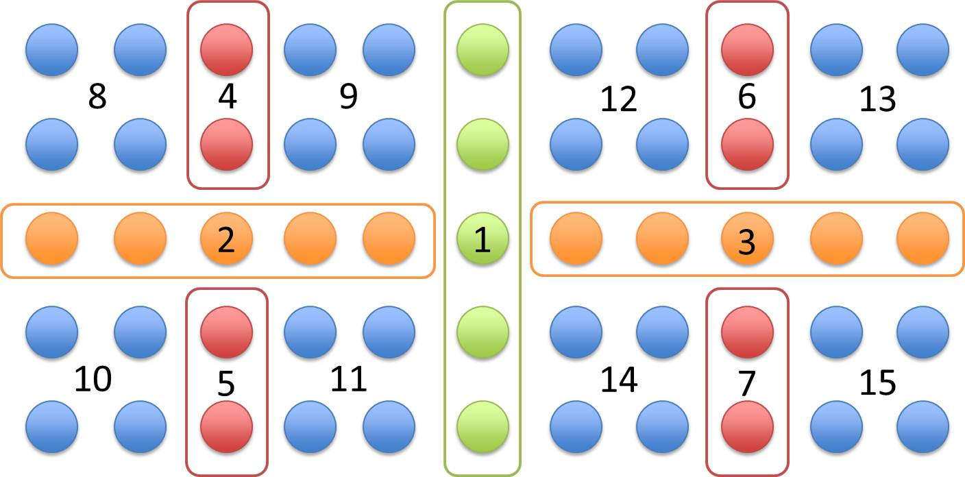
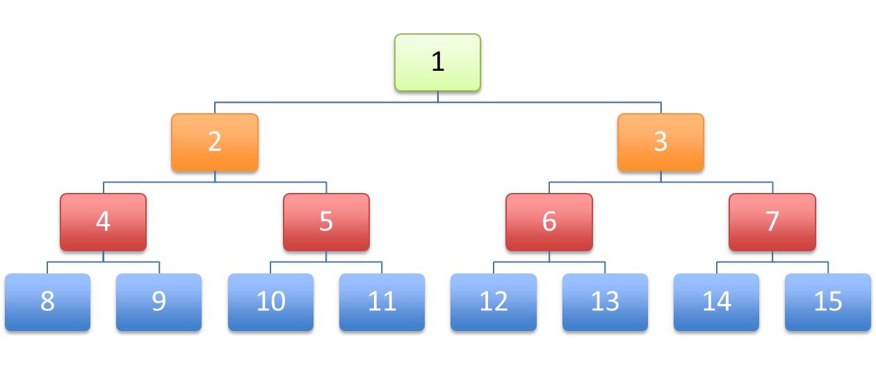
Figure 4: Example of a multilevel partition.

Based on the hierarchical structure of the tree, let $P_{i}$ denote the set of all cluster indices $j$ such that cluster $j$ is an ancestor of cluster $i$. For example for Figure 4, $P_{5}$ is equal to $\left\{1,2\right\}$ and $P_{15}=\left\{1,3,7\right\}$. Let $C_{i}$ denote the set of all cluster indices $j$ such that cluster $j$ is a descendant of cluster $i$. For the partition on Figure 4, $C_{4}$ is equal to $\left\{8,9\right\}$ and $C_{3}=\left\{6,7,12,13,14,15\right\}$. Note that a cluster may or may not have a direct coupling in the matrix $\mathbf{A}$ to any of its ancestors or descendants.

Once the partition is set, the algorithm may be separated into two distinct parts: computation of $\mathbf{G}^{r}$ and computation of $\mathbf{G}^{<}$.

Computation of blocks for $\mathbf{G}^{r}$

In the binary tree, the levels are labeled from bottom to top, where level 1 contains all clusters at the end of the tree and level $L$ contains only the original separator. For simplicity of presentation, let $\mathbf{A}^{(l)}$ denote the matrix transformed from $\mathbf{A}$ after folding all the clusters up to level $l$. Note that $\mathbf{A}^{(0)}$ is set to $\mathbf{A}$ and $\mathbf{A}^{(L-1)}$ is block diagonal.

The computation of blocks for $\mathbf{G}^{r}$ involve three steps: folding the lower level clusters unto the higher ones, inversion of the matrix for the main separator, and extracting of the diagonal blocks for the current level from blocks on higher level.

The algorithm for the first step goes as follows:

• For $l=1$ up to $L-1$,

  • $\mathbf{A}^{(l)}=\mathbf{A}^{(l-1)}$

  • For all the clusters $i$ on level $l$,

    • $\boldsymbol{\Psi}_{i,j}=-\left(\mathbf{A}_{i,i}^{(l)}\right)^{-1}\mathbf{A}_{i,j}^{(l)}$ for all $j$ in $P_{i}$

    • $\mathbf{A}_{j,k}^{(l)}=\mathbf{A}_{j,k}^{(l)}+\boldsymbol{\Psi}_{i,j}^{T}\mathbf{A}_{i,k}^{(l)}$ for all $j$ and $k$ in $P_{i}$

    • $\mathbf{A}_{k,j}^{(l)}=\left(\mathbf{A}_{j,k}^{(l)}\right)^{T}$ for all $j$ and $k$ in $P_{i}$

    • $\mathbf{A}_{i,j}^{(l)}=\mathbf{0}$ and $\mathbf{A}_{j,i}^{(l)}=\mathbf{0}$ for all $j$ in $P_{i}$

  • end

• end

The next step is written as the inversion of $\mathbf{A}^{(L-1)}$ , which is symmetric and block diagonal.

• $\mathbf{G}^{(L-1)}=\left(\mathbf{A}^{(L-1)}\right)^{-1}$

In practice, the operation requires only the inversion of the block for the top separator. All the other blocks have already been inverted during the folding steps.

Finally, all the diagonal blocks of $\mathbf{G}^{r}$ are extracted one level at a time. The algorithm goes as follows:

• For $l=L-2$ down to $0$,

  • $\mathbf{G}^{(l)}=\mathbf{G}^{(l+1)}$

  • For all the clusters $i$ on level $l$,

    • $\mathbf{G}_{i,j}^{(l)}=\mathbf{G}_{i,j}^{(l)}+\sum_{k\in P_{i}}\boldsymbol{\Psi}_{i,k}\mathbf{G}_{k,j}^{(l)}$ for all cluster indices $j$ in $P_{i}$

    • $\mathbf{G}_{j,i}^{(l)}=\left(\mathbf{G}_{i,j}^{(l)}\right)^{T}$ for all cluster indices $j$ in $P_{i}$

    • $\mathbf{G}_{i,i}^{(l)}=\mathbf{G}_{i,i}^{(l)}+\sum_{j\in P_{i}}\boldsymbol{\Psi}_{i,j}\mathbf{G}_{j,i}^{(l)}$

  • end

• end

The resulting algorithm to compute block entries in $\mathbf{G}^{r}$ matches exactly the HSC method [14].

Note that matrix $\mathbf{G}^{(0)}$ is not equal to $\mathbf{G}^{r}$ because $\mathbf{G}^{(0)}$ is incomplete (see an example in the Appendix). However, all the entries in $\mathbf{G}^{(0)}$, in particular the diagonal entries, match the corresponding entries in $\mathbf{G}^{r}$.

Computation of blocks for $\mathbf{G}^{<}$

The algorithm consists of four steps. The first step uses the matrix $\mathbf{G}^{(0)}$ computed previously.

• $\mathbf{N}=\boldsymbol{\Sigma}^{<}\left(\mathbf{G}^{(0)}\right)^{\dagger}$

All the entries in $\mathbf{G}^{(0)}$ match the corresponding entries in $\mathbf{G}^{r}$ and are sufficient to compute diagonal blocks of $\mathbf{G}^{<}$. The matrix $\mathbf{\Sigma}^{<}$ is typically block diagonal. The matrix $\mathbf{N}$ will have the same structure and shape as $\mathbf{G}^{(0)}$. The matrix multiplication is done block by block.

Next the lower level clusters are folded into the higher ones. This step is critical and the most time consuming. Let $\mathbf{N}^{(l)}$ denote the matrix transformed from $\mathbf{N}$ after folding all the clusters up to level $l$. $\mathbf{N}^{(0)}$ is set to $\mathbf{N}$.

• For $l=1$ up to $L-1$,

  • $\mathbf{N}^{(l)}=\mathbf{N}^{(l-1)}$

  • For all the clusters $i$ on level $l$,

    • $\mathbf{N}_{j,k}^{(l)}=\mathbf{N}_{j,k}^{(l)}+\boldsymbol{\Psi}_{i,j}^{T}\mathbf{N}_{i,k}^{(l)}$ for all $j$ and $k$ in $P_{i}$

  • end

• end

Similarly to Step 1, Step 3 is a block diagonal multiplication.

• $\mathbf{P}^{(L-1)}=\mathbf{G}^{(L-1)}\mathbf{N}^{(L-1)}$

Finally, Step 4 extracts all the diagonal blocks one level at a time. This step is similar to the extraction in the $\mathbf{G}^{r}$ algorithm. The operations are the following:

• For $l=L-2$ down to $0$,

  • $\mathbf{P}^{(l)}=\mathbf{P}^{(l+1)}$

  • For all the clusters $i$ on level $l$,

    • $\mathbf{P}_{i,j}^{(l)}=\mathbf{P}_{i,j}^{(l)}+\sum_{k\in P_{i}}\boldsymbol{\Psi}_{i,k}\mathbf{P}_{k,j}^{(l)}$ for all cluster indices $j$ in $P_{i}$

    • $\mathbf{P}_{j,i}^{(l)}=-\left(\mathbf{P}_{i,j}^{(l)}\right)^{\dagger}$ for all cluster indices $j$ in $P_{i}$

    • $\mathbf{P}_{i,i}^{(l)}=\mathbf{P}_{i,i}^{(l)}+\sum_{j\in P_{i}}\boldsymbol{\Psi}_{i,j}\mathbf{P}_{j,i}^{(l)}$

  • end

• end

At the end, matrix $\mathbf{P}^{(0)}$ is not equal to $\mathbf{G}^{<}$ because $\mathbf{P}^{(0)}$ is incomplete (see an example in the Appendix). However, all the entries in $\mathbf{P}^{(0)}$, in particular the diagonal entries, match the corresponding entries in $\mathbf{G}^{<}$.

Comments on the system partition

The partitioning of the system (or the clustering of points) is the key step for the efficiency of this algorithm. The partition should follow two rules:

1. for clusters within the same level on the binary tree, no interaction is allowed. Operations on blocks at the same level are performed independently.

2. the partition should minimize the size of separators and reduce the clusters down to a size manageable for an inversion of the corresponding block matrix.

The multilevel nested dissection generates a partition that satisfies those rules. It is worthwhile to note that, as long as the rules stated above are followed, systems with non-uniform distribution of points or with a different stencil could be treated correctly.

The RGF algorithm is included in the previous description with a very specific partition. Such a partition is illustrated in Figure 5.

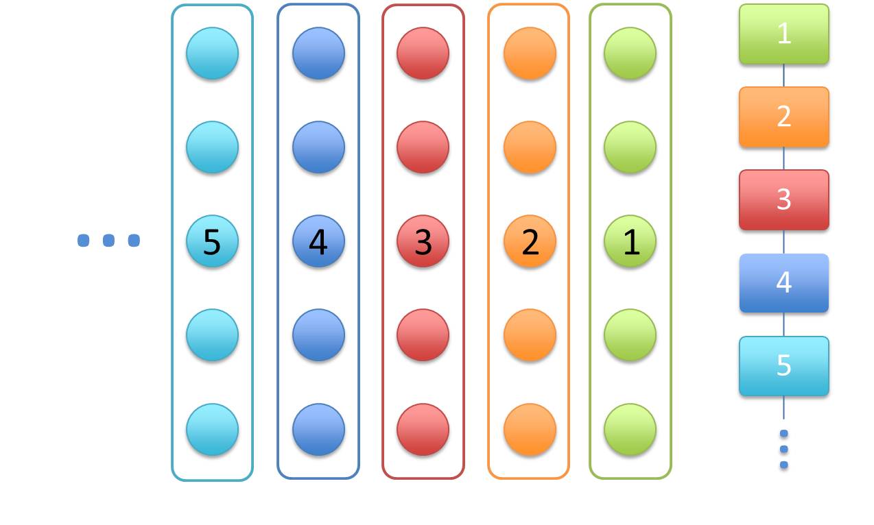
Figure 5: Partition generating the RGF algorithm.

In many cases, self-energy functions add two $N_{x}\times N_{x}$ dense blocks into the input sparse matrix $\mathbf{A}$ in first and last block (see Figure 2). One possible partition combines the two contacts together with the middle separator 1, as shown in Figure 6.

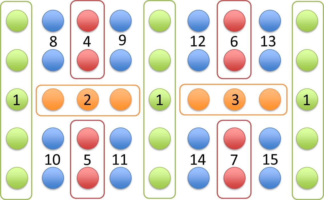
Figure 6: First method to partition system with two dense layers and two ends.

The weakness of such clustering is the size of the first separator (or root region). A larger separator increases the computational cost spent on this level. More descendant blocks are coupled with this separator and the total number of operations will increase dramatically. Another partition that satisfies the previous two rules is plotted in Figure 7.

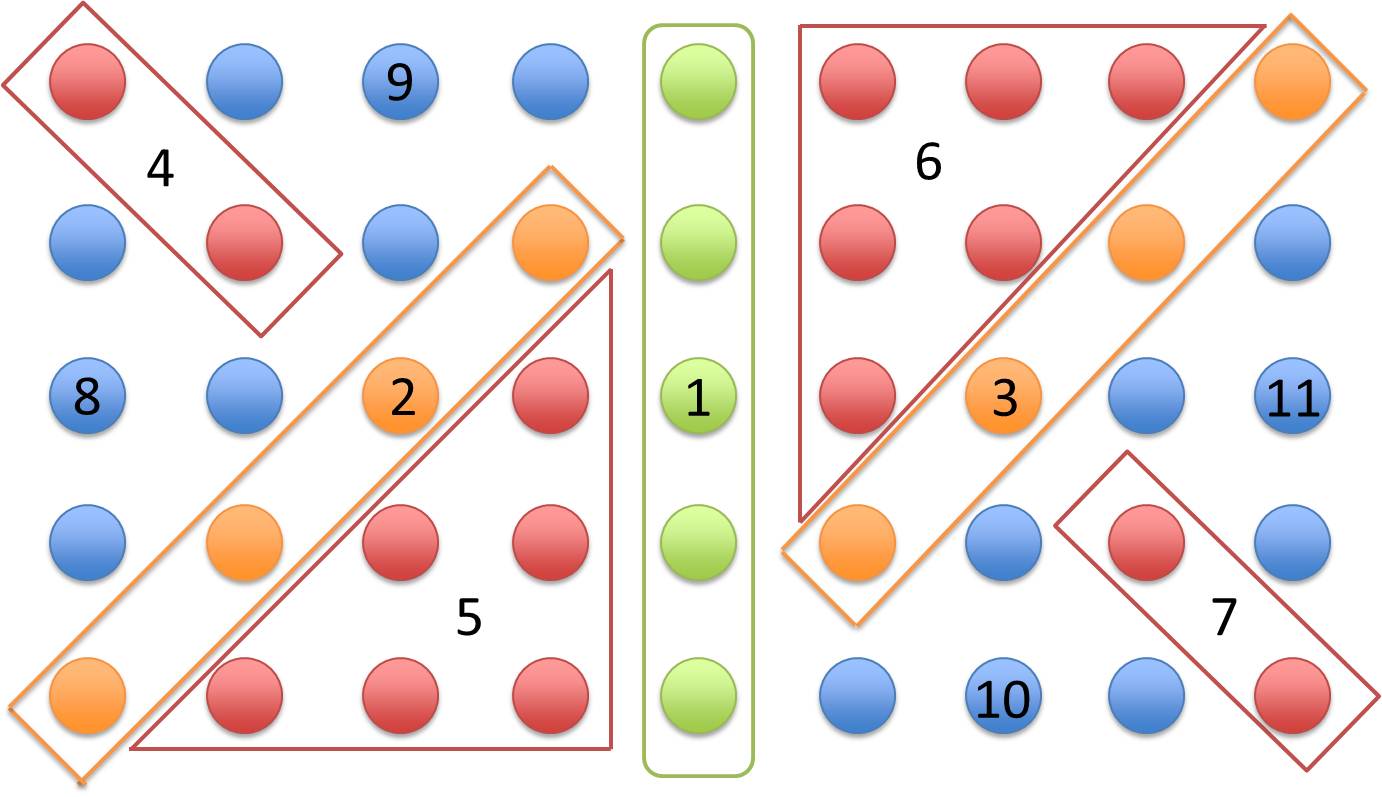
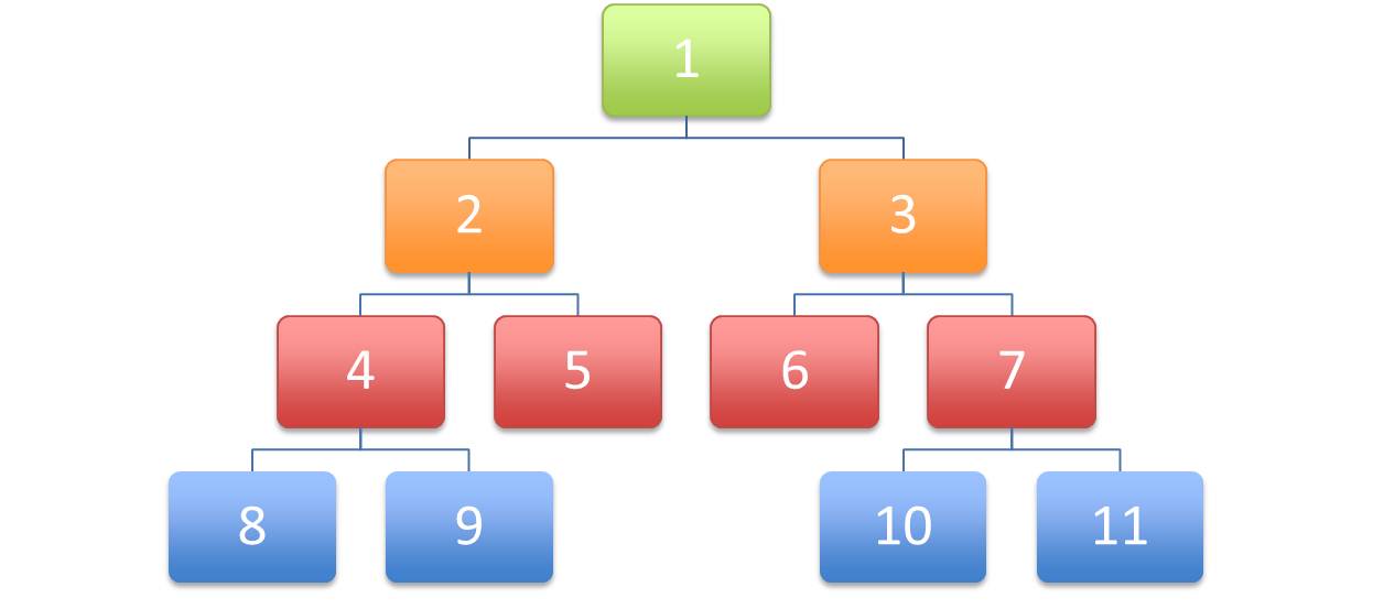
Figure 7: Partition generated by METIS for system including dense layers at two ends.

4 Numerical Experiments

This section describes numerical experiments on two simple models: a super-lattice structure and a graphene nanotube. The algorithm is implemented in a C code that is interfaced with METIS [9].

4.1 Cost analysis

First the complexity of the HSC extension is compared numerically to the complexity of RGF. A model device is considered where the system Hamiltonian is discretized with a five-point stencil. The left and right contact self-energies are neglected for this section only. A typical partition is plotted in Figure 4.

The numerical estimate tracks the operation counts step by step for all the matrix multiplications and matrix inversions throughout the code. For a multiplication of two matrices with dimensions $i\times j$ and $j\times k$, a total of $ijk$ operations is added. For inversion of a matrix of dimension $i\times i$, $i^{3}$ operations are counted.

Figure 8 shows the cost comparison between the HSC extension and RGF for two-dimensional square systems with the same number of grid points (or atoms) per direction, i.e. $N_{x}=N_{y}=N$. The plot in logarithmic scale indicates that RGF exhibits a complexity of $\mathcal{O}(N^{4})$, while the HSC-extension shows a $\mathcal{O}(N^{3})$ complexity.

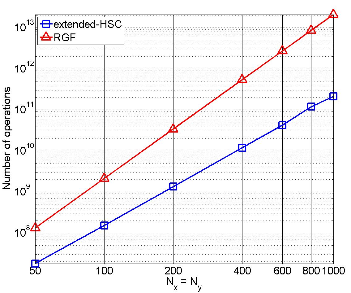
Figure 8: Numerical count comparison for our algorithm (blue) and RGF (red).

4.2 Results

4.2.1 Super-lattice device

A super-lattice device is typically a multi-layered energy barriers system. The device is composed of repeating junctions of energy barriers and wells. To verify the simulation results, a two-dimensional system of lengths $l_{x}=25\mathrm{nm}$ and $l_{y}=20\mathrm{nm}$ is considered and plotted in Figure 9. Here the structure has eight barriers, each of width $1\mathrm{nm}$ and of height 400meV. The wells have a width of 1nm. The length of the left flat band region is $2\mathrm{nm}$ and the right flat band region is 3nm long.

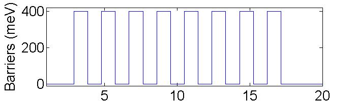
Figure 9: Barrier structure for a model super-lattice device.

A simulation with a five-point stencil discretization on a grid with spacing $\mathrm{d}x=\mathrm{d}y=0.1\mathrm{nm}$ is made for the Fermi energy $E_{f}=140\mathrm{meV}$ and 500 energy points uniformly distributed between 0 to $500\mathrm{meV}$. The density of states, electron density, and current are calculated by the RGF method and the extended-HSC method. The output electron density is plotted in Figure 10. Linear electron density in the $y$-direction is illustrated in Figure 11. The figures indicate that the charge distribution in the barrier-well multi-layer junctions are symmetric, as expected.

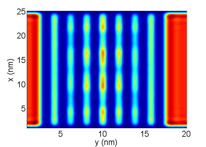
Figure 10: Electron density for a model super-lattice device.

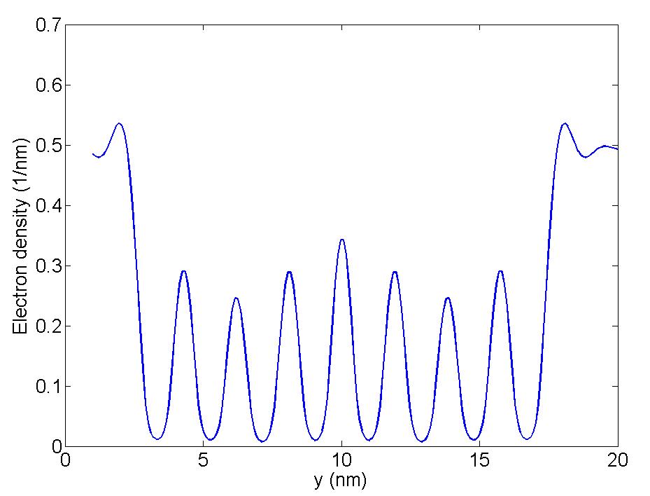
Figure 11: Electron density in $y$ direction of the example super-lattice structure.

Next devices of lengths $l_{x}=N_{x}\times 0.1\mathrm{nm}$ and $l_{y}=N_{y}\times 0.1\mathrm{nm}$ are used to compare the two algorithms. The number of barriers is kept at 8. The lengths for the two-sides flat region are adjusted according to the lengths of device $l_{x}$ and $l_{y}$. The other parameters remain unchanged.

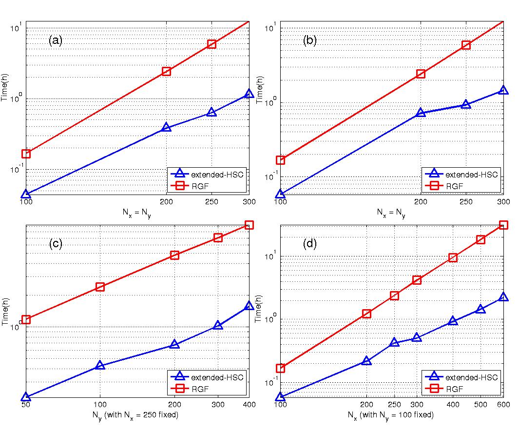
Figure 12: Superlattice device NEGF simulation computation time comparison for RGF and our methods, all systems grid spacing is 0.1nm. (a) Square system of with diagonal self-energy matrix; (b) Square system of with dense self-energy matrix; (c) For systems in this plot, the length in the $x$-direction is fixed at 25nm while the length in the $y$-direction is increased. (d) For systems in this plot, the length in the $y$-direction is fixed at 10nm while the length in the $x$-direction is increased. Dense self-energy matrices are used in (c) and (d) devices.

In Figure 12(a), diagonal self-energy matrices are used for the left and right contacts. Calculation times are compared for square systems— i.e. $N_{x}=N_{y}=N$ — and plotted in Figure 12(a). As expected, the HSC-extension exhibits smaller CPU times and a complexity of $\mathcal{O}(N^{3})$ while RGF’s complexity is $\mathcal{O}(N^{4})$.

In Figure 12(b), CPU times for square systems with dense self-energy matrices for both contacts are plotted. Here again the HSC-extension exhibits smaller CPU times. A complexity $\mathcal{O}(N^{3})$ for HSC-extension compared with $\mathcal{O}(N^{4})$ for RGF can be seen.

Figure 12(c) plots CPU times for rectangular devices where $l_{x}=25\mathrm{nm}$ (or $N_{x}=250$) and the length in the $y$-direction is varied. Dense self-energy blocks for the left and right contacts are employed. The implementation of RGF is biased towards the $x$-direction so that its complexity is $\mathcal{O}\left(N_{y}\right)$. The linear trend is clearly present in the plot. For the HSC-extension, similarly to the cost of a sparse $\mathbf{LDL}^{T}$ factorization, the computational cost is $\mathcal{O}\left(N_{y}\right)$. Clearly, the constant for RGF is larger for this device.

To illustrate the dependence of this constant with respect to $N_{x}$, Figure 12(d) plots the CPU times when $N_{y}$ is fixed and $N_{x}$ is varied. The recorded CPU times illustrate that the RGF method has an asymptotic complexity $\mathcal{O}\left(N_{x}^{3}\right)$, while the HSC extension exhibits a complexity $\mathcal{O}\left(N_{x}^{2}\right)$. So, for rectangular devices, the RGF method has a complexity $\mathcal{O}(N_{x}^{3}N_{y})$ and the HSC-extension a complexity $\mathcal{O}(N_{x}^{2}N_{y})$.

4.2.2 Graphene

Graphene is one of the most promising next-generation materials. Its remarkable electric properties, such as high carrier mobility and zero band gaps, generate a rapidly increasing interest in the electronic device community. Since 2007, many advances in graphene-based transistor development have been reported. [19]

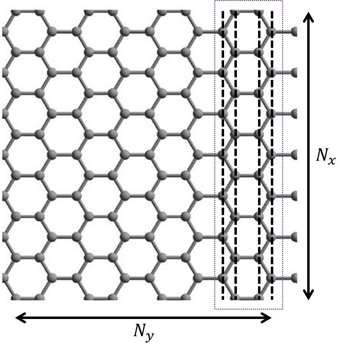
Figure 13: Graphene hexagonal structure decomposed by tight biding method. Dashed rectangular illustrates one repeating hexagon layer. Dashed lines represent inner four atom layers, showing the atoms ordering in tight binding Hamiltonian construction.

The NEGF simulation of graphene transport is based on tight binding method, which yields a four-point-stencil Hamiltonian due to system decomposition of carbon atoms coupling (see Figure 13). In the numerical experiments, armchair planar graphene nanoribbon structures are simulated. The on-site energy for each carbon atom is 0 and the hopping parameter between two nearest carbon atoms is -3.1eV. The Fermi energy is set to 0. The simulation is run for only one energy point $E=0.5$eV.

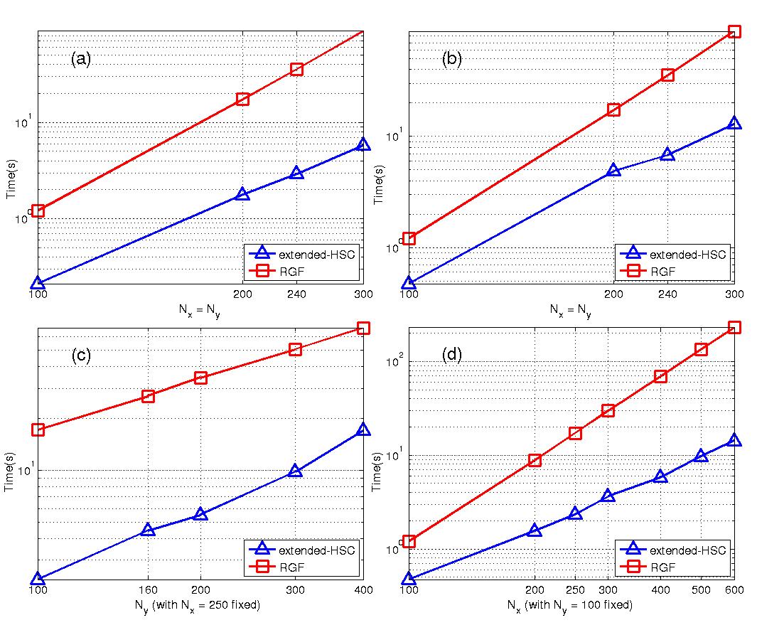
Figure 14: Graphene device NEGF simulation computation time comparison for RGF and the HSC extension, based on tight binding theory. (a) Square system of with diagonal self-energy matrix. (b) Square system of with dense self-energy matrix. (c) For systems in this plot, the number of atoms in the $x$-direction is set to $N_{x}=250$, while the number of atoms in the $y$-direction is increased. (d) For systems in this plot, the number of atoms in the $y$-direction is set to $N_{y}=100$, while the number of atoms in the $x$-direction is increased. Dense self-energy matrices are used in (c) and (d) devices.

Simulation timings are plotted in Figure 14 for graphene structures of different sizes. To minimize the dimension of blocks to invert in RGF, one layer of hexagonal structure is divided into four layers (see the dashed lines in Figure 13). Conclusions on the asymptotic complexity remain unchanged. Namely, the HSC extension is more efficient than the RGF method for square and rectangular structures. The complexity of RGF for four-point stencil behaves as $\mathcal{O}(N_{x}^{3}N_{y})$ with the same constant as five-point stencil, which is expected due to the layered system partition. In Figure 14(a) and (b), for a four-point stencil system, our HSC-extension exhibits a complexity of $\mathcal{O}(N^{3})$ for square system. Figure 14(c) and (d) also demonstrate a complexity growing linearly with $N_{y}$ and, respectively quadratically with $N_{x}$, when $N_{x}$, respectively $N_{y}$, is fixed. The final result is a complexity $\mathcal{O}(N_{x}^{2}N_{y})$. The constant in front of $N_{x}^{2}N_{y}$ for the extended HSC method is smaller for the graphene structures than for the superlattice devices. This reduction is explained by a more efficient partitioning of four-point stencil systems by METIS .

5 Conclusion

In this paper, an approach to calculate the charge density in nanoscale devices, within the context of the non equilibrium Green’s function approach, is presented. This work exploits recent advances to use an established graph partitioning method, namely the nested dissection method. This contribution does not require any processing of the partition and it can handle open boundary conditions, represented by full self-energy matrices. The key ingredients are an efficient sparse block $\mathbf{LDL}^{T}$-factorization and an appropriate order of operations to preserve the sparsity as much as possible. The resulting algorithm was illustrated on a quantum well superlattice and a carbon nanotube, which are represented by a continuum and tight binding Hamiltonian respectively, and demonstrated a significant speed up over the recursive method RGF.

Appendix A Description of the Algorithm for a Three-level Tree

In order to make the extension more comprehensive, a description of the HSC extension is given for a three-level system (see Figure 15).

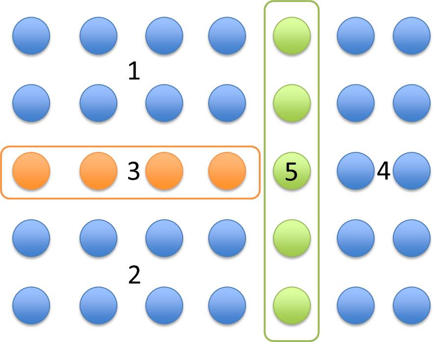
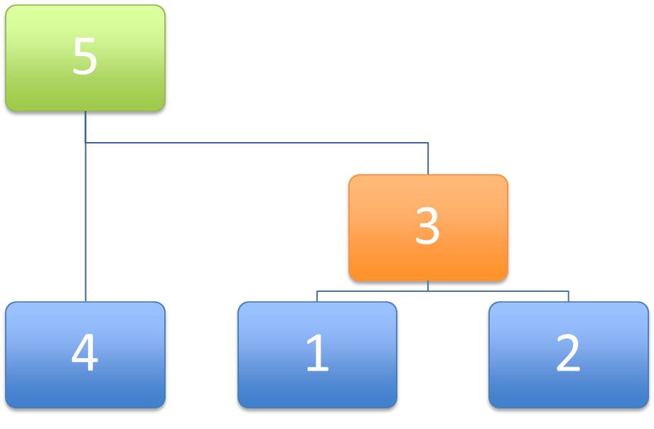
Figure 15: Partition for a three-level system.

The size of the partition is chosen to make the description as relevant as possible without becoming overcomplicated. The first level contains regions 1, 2, and 4. The second-level refers to region 3 and the top level is the root or region 5. To illustrate the algorithm, steps from Section 3.2 are described for this particular device.

When a five-point stencil is used for discretization, the structure of the matrix $\mathbf{A}$, after re-ordering, is

$$\mathbf{A}=\left[\begin{array}[]{ccccc}\mathbf{A}_{11}&\mathbf{0}&\mathbf{A}_{13}&\mathbf{0}&\mathbf{A}_{15}\\ \mathbf{0}&\mathbf{A}_{22}&\mathbf{A}_{23}&\mathbf{0}&\mathbf{A}_{25}\\ \mathbf{A}_{13}^{T}&\mathbf{A}_{23}^{T}&\mathbf{A}_{33}&\mathbf{0}&\mathbf{A}_{35}\\ \mathbf{0}&\mathbf{0}&\mathbf{0}&\mathbf{A}_{44}&\mathbf{A}_{45}\\ \mathbf{A}_{15}^{T}&\mathbf{A}_{25}^{T}&\mathbf{A}_{35}^{T}&\mathbf{A}_{45}^{T}&\mathbf{A}_{55}\end{array}\right]$$

The blocks $\mathbf{A}_{11}$ and $\mathbf{A}_{44}$ are dense for representing the contacts with the semi-infinite leads.

Recall that $\mathbf{A}^{(0)}$ is equal to $\mathbf{A}$. Then inner points in regions 1, 2, and 4 are eliminated by block Gaussian elimination — the effects of the inner points in regions 1, 2, and 4 are folded over their boundary. This first step yields the matrix $\mathbf{A}^{(1)}$

$$\mathbf{A}^{(1)}=\left[\begin{array}[]{ccccc}\mathbf{A}_{11}&\mathbf{0}&\mathbf{0}&\mathbf{0}&\mathbf{0}\\ \mathbf{0}&\mathbf{A}_{22}&\mathbf{0}&\mathbf{0}&\mathbf{0}\\ \mathbf{0}&\mathbf{0}&\mathbf{A}_{33}^{(1)}&\mathbf{0}&\mathbf{A}_{35}^{(1)}\\ \mathbf{0}&\mathbf{0}&\mathbf{0}&\mathbf{A}_{44}&\mathbf{0}\\ \mathbf{0}&\mathbf{0}&\left(\mathbf{A}_{35}^{(1)}\right)^{T}&\mathbf{0}&\mathbf{A}_{55}^{(1)}\end{array}\right]$$

where the updated matrices are

$$\mathbf{A}_{33}^{(1)} =\mathbf{A}_{33}-\mathbf{A}_{13}^{T}\mathbf{A}_{11}^{-1}\mathbf{A}_{13}-\mathbf{A}_{23}^{T}\mathbf{A}_{22}^{-1}\mathbf{A}_{23},$$

$$\mathbf{A}_{35}^{(1)} =\mathbf{A}_{35}-\mathbf{A}_{13}^{T}\mathbf{A}_{11}^{-1}\mathbf{A}_{15}-\mathbf{A}_{23}^{T}\mathbf{A}_{22}^{-1}\mathbf{A}_{25},$$

$$\mathbf{A}_{55}^{(1)} =\mathbf{A}_{55}-\mathbf{A}_{15}^{T}\mathbf{A}_{11}^{-1}\mathbf{A}_{15}-\mathbf{A}_{25}^{T}\mathbf{A}_{22}^{-1}\mathbf{A}_{25}-\mathbf{A}_{45}^{T}\mathbf{A}_{44}^{-1}\mathbf{A}_{45}.$$

After folding the effects of regions 1 and 2, block $\mathbf{A}_{35}^{(1)}$ is now a dense block. Figure 16 illustrates the change of sparsity between $\mathbf{A}$ and $\mathbf{A}^{(1)}$.

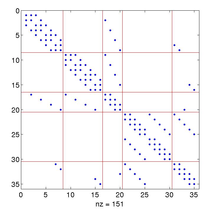
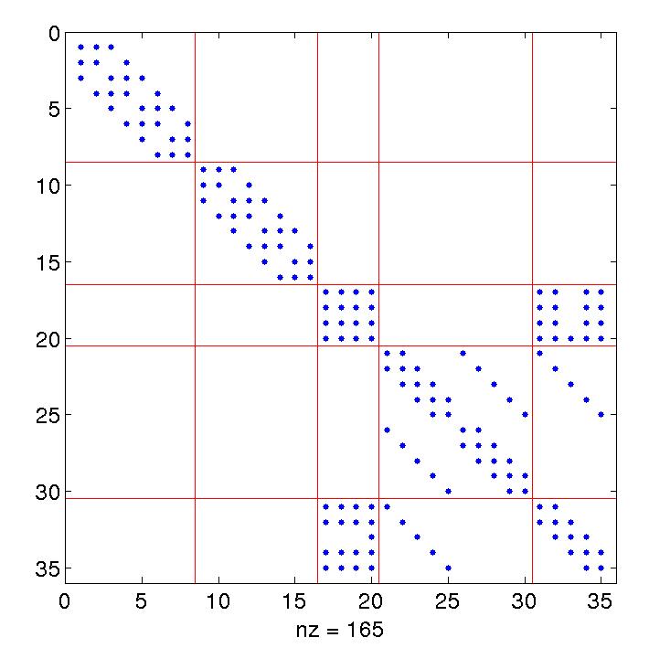
Figure 16: Sparsity of matrix $\mathbf{A}$ and matrix $\mathbf{A}^{(1)}$.

In the next step, the remaining off-diagonal blocks are eliminated to obtain the matrix $\mathbf{A}^{(2)}$,

$$\mathbf{A}^{(2)}=\left[\begin{array}[]{ccccc}\mathbf{A}_{11}&\mathbf{0}&\mathbf{0}&\mathbf{0}&\mathbf{0}\\ \mathbf{0}&\mathbf{A}_{22}&\mathbf{0}&\mathbf{0}&\mathbf{0}\\ \mathbf{0}&\mathbf{0}&\mathbf{A}_{33}^{(1)}&\mathbf{0}&\mathbf{0}\\ \mathbf{0}&\mathbf{0}&\mathbf{0}&\mathbf{A}_{44}&\mathbf{0}\\ \mathbf{0}&\mathbf{0}&\mathbf{0}&\mathbf{0}&\mathbf{A}_{55}^{(2)}\end{array}\right]$$

where the block $\mathbf{A}_{55}^{(2)}$ is

$$\mathbf{A}_{55}^{(2)}=\mathbf{A}_{55}^{(1)}-\left(\mathbf{A}_{35}^{(1)}\right)^{T}\left(\mathbf{A}_{33}^{(1)}\right)^{-1}\mathbf{A}_{35}^{(1)}.$$

Note that several blocks are unchanged, like $\mathbf{A}_{11}$, $\mathbf{A}_{22}$, $\mathbf{A}_{33}^{(1)}$, and $\mathbf{A}_{44}$. The next step is written as the inversion of $\mathbf{A}^{(2)}$, which is symmetric and block diagonal,

$$\mathbf{G}^{(2)}=\left[\begin{array}[]{ccccc}\mathbf{A}_{11}^{-1}&\mathbf{0}&\mathbf{0}&\mathbf{0}&\mathbf{0}\\ \mathbf{0}&\mathbf{A}_{22}^{-1}&\mathbf{0}&\mathbf{0}&\mathbf{0}\\ \mathbf{0}&\mathbf{0}&\left(\mathbf{A}_{33}^{(1)}\right)^{-1}&\mathbf{0}&\mathbf{0}\\ \mathbf{0}&\mathbf{0}&\mathbf{0}&\mathbf{A}_{44}^{-1}&\mathbf{0}\\ \mathbf{0}&\mathbf{0}&\mathbf{0}&\mathbf{0}&\left(\mathbf{A}_{55}^{(2)}\right)^{-1}\end{array}\right].$$

This operation requires only the inversion of the block $\mathbf{A}_{55}^{(2)}$. All the other blocks have been inverted during the folding steps.

Next diagonal blocks of $\mathbf{G}^{r}$ are extracted one level at a time. Starting from the main root (or separator), blocks at level 2 are updated to obtain

$$\mathbf{G}^{(1)}=\left[\begin{array}[]{ccccc}\mathbf{G}_{11}^{(2)}&\mathbf{0}&\mathbf{0}&\mathbf{0}&\mathbf{0}\\ \mathbf{0}&\mathbf{G}_{22}^{(2)}&\mathbf{0}&\mathbf{0}&\mathbf{0}\\ \mathbf{0}&\mathbf{0}&\mathbf{G}_{33}^{(1)}&\mathbf{0}&\mathbf{G}_{35}^{(1)}\\ \mathbf{0}&\mathbf{0}&\mathbf{0}&\mathbf{G}_{44}^{(2)}&\mathbf{0}\\ \mathbf{0}&\mathbf{0}&\left(\mathbf{G}_{35}^{(1)}\right)^{T}&\mathbf{0}&\mathbf{G}_{55}^{(2)}\end{array}\right]$$

with

$$\mathbf{G}_{35}^{(1)} =-\left(\mathbf{A}_{33}^{(1)}\right)^{-1}\mathbf{A}_{35}^{(1)}\mathbf{G}_{55}^{(2)}=\boldsymbol{\Psi}_{35}\mathbf{G}_{55}^{(2)},$$

$$\mathbf{G}_{33}^{(1)} =\mathbf{G}_{33}^{(2)}-\left(\mathbf{A}_{33}^{(1)}\right)^{-1}\mathbf{A}_{35}^{(1)}\left(\mathbf{G}_{35}^{(1)}\right)^{T}=\mathbf{G}_{33}^{(2)}+\boldsymbol{\Psi}_{35}\left(\mathbf{G}_{35}^{(1)}\right)^{T}.$$

Finally, blocks for regions 1, 2, and 4 are updated, yielding the matrix $\mathbf{G}^{(0)}$,

$$\mathbf{G}^{(0)}=\left[\begin{array}[]{ccccc}\mathbf{G}_{11}^{(0)}&\mathbf{0}&\mathbf{G}_{13}^{(0)}&\mathbf{0}&\mathbf{G}_{15}^{(0)}\\ \mathbf{0}&\mathbf{G}_{22}^{(0)}&\mathbf{G}_{23}^{(0)}&\mathbf{0}&\mathbf{G}_{25}^{(0)}\\ \left(\mathbf{G}_{13}^{(0)}\right)^{T}&\left(\mathbf{G}_{23}^{(0)}\right)^{T}&\mathbf{G}_{33}^{(1)}&\mathbf{0}&\mathbf{G}_{35}^{(1)}\\ \mathbf{0}&\mathbf{0}&\mathbf{0}&\mathbf{G}_{44}^{(0)}&\mathbf{G}_{45}^{(0)}\\ \left(\mathbf{G}_{15}^{(0)}\right)^{T}&\left(\mathbf{G}_{25}^{(0)}\right)^{T}&\left(\mathbf{G}_{35}^{(1)}\right)^{T}&\left(\mathbf{G}_{45}^{(0)}\right)^{T}&\mathbf{G}_{55}^{(2)}\end{array}\right].$$

Blocks for region 4 are satisfying

$$\mathbf{G}_{45}^{(0)} =-\left(\mathbf{A}_{44}^{(0)}\right)^{-1}\mathbf{A}_{45}^{(0)}\mathbf{G}_{55}^{(2)}=\boldsymbol{\Psi}_{45}\mathbf{G}_{55}^{(2)}$$

$$\mathbf{G}_{44}^{(0)} =\mathbf{G}_{44}^{(2)}-\left(\mathbf{A}_{44}^{(0)}\right)^{-1}\mathbf{A}_{45}^{(0)}\left(\mathbf{G}_{45}^{(0)}\right)^{T}$$

Blocks for region 1 are defined by

$$\mathbf{G}_{15}^{(0)} =-\left(\mathbf{A}_{11}^{(0)}\right)^{-1}\mathbf{A}_{15}^{(0)}\mathbf{G}_{55}^{(2)}-\left(\mathbf{A}_{11}^{(0)}\right)^{-1}\mathbf{A}_{13}^{(0)}\mathbf{G}_{35}^{(1)}$$

$$\mathbf{G}_{13}^{(0)} =-\left(\mathbf{A}_{11}^{(0)}\right)^{-1}\mathbf{A}_{13}^{(0)}\mathbf{G}_{33}^{(1)}-\left(\mathbf{A}_{11}^{(0)}\right)^{-1}\mathbf{A}_{15}^{(0)}\left(\mathbf{G}_{35}^{(1)}\right)^{T}$$

$$\mathbf{G}_{11}^{(0)} =\left(\mathbf{A}_{11}^{(0)}\right)^{-1}-\left(\mathbf{A}_{11}^{(0)}\right)^{-1}\mathbf{A}_{13}^{(0)}\left(\mathbf{G}_{13}^{(0)}\right)^{T}-\left(\mathbf{A}_{11}^{(0)}\right)^{-1}\mathbf{A}_{15}^{(0)}\left(\mathbf{G}_{15}^{(0)}\right)^{T}$$

and blocks for region 2

$$\mathbf{G}_{25}^{(0)} =-\left(\mathbf{A}_{22}^{(0)}\right)^{-1}\mathbf{A}_{25}^{(0)}\mathbf{G}_{55}^{(2)}-\left(\mathbf{A}_{22}^{(0)}\right)^{-1}\mathbf{A}_{23}^{(0)}\mathbf{G}_{35}^{(1)}$$

$$\mathbf{G}_{23}^{(0)} =-\left(\mathbf{A}_{22}^{(0)}\right)^{-1}\mathbf{A}_{23}^{(0)}\mathbf{G}_{33}^{(1)}-\left(\mathbf{A}_{22}^{(0)}\right)^{-1}\mathbf{A}_{25}^{(0)}\left(\mathbf{G}_{35}^{(1)}\right)^{T}$$

$$\mathbf{G}_{22}^{(0)} =\left(\mathbf{A}_{22}^{(0)}\right)^{-1}-\left(\mathbf{A}_{22}^{(0)}\right)^{-1}\mathbf{A}_{23}^{(0)}\left(\mathbf{G}_{23}^{(0)}\right)^{T}-\left(\mathbf{A}_{22}^{(0)}\right)^{-1}\mathbf{A}_{25}^{(0)}\left(\mathbf{G}_{25}^{(0)}\right)^{T}$$

Figure 17 displays the sparsity of the resulting matrix $\mathbf{G}^{(0)}$.

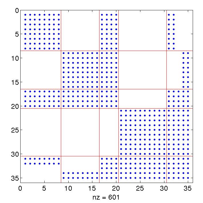
Figure 17: Sparsity of matrix $\mathbf{G}^{(0)}$.

All the entries in $\mathbf{G}^{(0)}$ are equal to their corresponding entries in $\mathbf{G}^{r}$.

The computation of diagonal blocks in $\mathbf{G}^{<}$ are described for the same device. First the matrix $\mathbf{N}$ is computed,

$$\mathbf{N}=\boldsymbol{\Sigma}^{<}\left(\mathbf{G}^{<}\right)^{\dagger}=\left[\begin{array}[]{ccccc}\boldsymbol{\Sigma}_{11}^{<}\overline{\mathbf{G}_{11}^{(0)}}&\mathbf{0}&\boldsymbol{\Sigma}_{11}^{<}\overline{\mathbf{G}_{13}^{(0)}}&\mathbf{0}&\boldsymbol{\Sigma}_{11}^{<}\overline{\mathbf{G}_{15}^{(0)}}\\ \mathbf{0}&\boldsymbol{\Sigma}_{22}^{<}\overline{\mathbf{G}_{22}^{(0)}}&\boldsymbol{\Sigma}_{22}^{<}\overline{\mathbf{G}_{23}^{(0)}}&\mathbf{0}&\boldsymbol{\Sigma}_{22}^{<}\overline{\mathbf{G}_{25}^{(0)}}\\ \boldsymbol{\Sigma}_{33}^{<}\left(\mathbf{G}_{13}^{(0)}\right)^{\dagger}&\boldsymbol{\Sigma}_{33}^{<}\left(\mathbf{G}_{23}^{(0)}\right)^{\dagger}&\boldsymbol{\Sigma}_{33}^{<}\overline{\mathbf{G}_{33}^{(0)}}&\mathbf{0}&\boldsymbol{\Sigma}_{33}^{<}\overline{\mathbf{G}_{35}^{(0)}}\\ \mathbf{0}&\mathbf{0}&\mathbf{0}&\boldsymbol{\Sigma}_{44}^{<}\overline{\mathbf{G}_{44}^{(0)}}&\boldsymbol{\Sigma}_{44}^{<}\overline{\mathbf{G}_{45}^{(0)}}\\ \boldsymbol{\Sigma}_{55}^{<}\left(\mathbf{G}_{15}^{(0)}\right)^{\dagger}&\boldsymbol{\Sigma}_{55}^{<}\left(\mathbf{G}_{25}^{(0)}\right)^{\dagger}&\boldsymbol{\Sigma}_{55}^{<}\left(\mathbf{G}_{35}^{(0)}\right)^{\dagger}&\boldsymbol{\Sigma}_{55}^{<}\left(\mathbf{G}_{45}^{(0)}\right)^{\dagger}&\boldsymbol{\Sigma}_{55}^{<}\overline{\mathbf{G}_{55}^{(0)}}\end{array}\right].$$

Set $\mathbf{N}^{(0)}=\mathbf{N}$. Next the lower level clusters are folded into the higher ones to obtain the matrix $\mathbf{N}^{(1)}$

$$\mathbf{N}^{(1)}=\left[\begin{array}[]{ccccc}\mathbf{N}_{11}^{(0)}&\mathbf{0}&\mathbf{N}_{13}^{(0)}&\mathbf{0}&\mathbf{N}_{15}^{(0)}\\ \mathbf{0}&\mathbf{N}_{22}^{(0)}&\mathbf{N}_{23}^{(0)}&\mathbf{0}&\mathbf{N}_{25}^{(0)}\\ \mathbf{N}_{31}^{(0)}&\mathbf{N}_{32}^{(0)}&\mathbf{N}_{33}^{(1)}&\mathbf{0}&\mathbf{N}_{35}^{(1)}\\ \mathbf{0}&\mathbf{0}&\mathbf{0}&\mathbf{N}_{44}^{(0)}&\mathbf{N}_{45}^{(0)}\\ \mathbf{N}_{51}^{(0)}&\mathbf{N}_{52}^{(0)}&\mathbf{N}_{53}^{(1)}&\mathbf{N}_{54}^{(0)}&\mathbf{N}_{55}^{(1)}\end{array}\right]$$

where the updated blocks are

$$\mathbf{N}_{33}^{(1)} =\mathbf{N}_{33}^{(0)}-\left(\mathbf{A}_{13}\right)^{T}\mathbf{A}_{11}^{-1}\mathbf{N}_{13}^{(0)}-\left(\mathbf{A}_{23}\right)^{T}\mathbf{A}_{22}^{-1}\mathbf{N}_{23}^{(0)}$$

$$\mathbf{N}_{55}^{(1)} =\mathbf{N}_{55}^{(0)}-\left(\mathbf{A}_{15}\right)^{T}\mathbf{A}_{11}^{-1}\mathbf{N}_{15}^{(0)}-\left(\mathbf{A}_{25}\right)^{T}\mathbf{A}_{22}^{-1}\mathbf{N}_{25}^{(0)}-\left(\mathbf{A}_{45}\right)^{T}\mathbf{A}_{44}^{-1}\mathbf{N}_{45}^{(0)}$$

$$\mathbf{N}_{35}^{(1)} =\mathbf{N}_{35}^{(0)}-\left(\mathbf{A}_{13}\right)^{T}\mathbf{A}_{11}^{-1}\mathbf{N}_{15}^{(0)}-\left(\mathbf{A}_{23}\right)^{T}\mathbf{A}_{22}^{-1}\mathbf{N}_{25}^{(0)}$$

$$\mathbf{N}_{53}^{(1)} =\mathbf{N}_{53}^{(0)}-\left(\mathbf{A}_{15}\right)^{T}\mathbf{A}_{11}^{-1}\mathbf{N}_{13}^{(0)}-\left(\mathbf{A}_{25}\right)^{T}\mathbf{A}_{22}^{-1}\mathbf{N}_{23}^{(0)}$$

For the top level, the block for region 5 is updated

$$\mathbf{N}^{(2)}=\left[\begin{array}[]{ccccc}\mathbf{N}_{11}^{(0)}&\mathbf{0}&\mathbf{N}_{13}^{(0)}&\mathbf{0}&\mathbf{N}_{15}^{(0)}\\ \mathbf{0}&\mathbf{N}_{22}^{(0)}&\mathbf{N}_{23}^{(0)}&\mathbf{0}&\mathbf{N}_{25}^{(0)}\\ \mathbf{N}_{31}^{(0)}&\mathbf{N}_{32}^{(0)}&\mathbf{N}_{33}^{(1)}&\mathbf{0}&\mathbf{N}_{35}^{(1)}\\ \mathbf{0}&\mathbf{0}&\mathbf{0}&\mathbf{N}_{44}^{(0)}&\mathbf{N}_{45}^{(0)}\\ \mathbf{N}_{51}^{(0)}&\mathbf{N}_{52}^{(0)}&\mathbf{N}_{53}^{(1)}&\mathbf{N}_{54}^{(0)}&\mathbf{N}_{55}^{(2)}\end{array}\right]$$

with

$$\mathbf{N}_{55}^{(2)}=\mathbf{N}_{55}^{(1)}-\left(\mathbf{A}_{35}^{(1)}\right)^{T}\left(\mathbf{A}_{33}^{(1)}\right)^{-1}\mathbf{N}_{35}^{(1)}.$$

The next step is a block-diagonal multiplication

$$\mathbf{P}^{(2)}=\left[\begin{array}[]{ccccc}\mathbf{A}_{11}^{-1}\mathbf{N}_{11}^{(0)}&\mathbf{0}&\mathbf{A}_{11}^{-1}\mathbf{N}_{13}^{(0)}&\mathbf{0}&\mathbf{A}_{11}^{-1}\mathbf{N}_{15}^{(0)}\\ \mathbf{0}&\mathbf{A}_{22}^{-1}\mathbf{N}_{22}^{(0)}&\mathbf{A}_{22}^{-1}\mathbf{N}_{23}^{(0)}&\mathbf{0}&\mathbf{A}_{22}^{-1}\mathbf{N}_{25}^{(0)}\\ \left(\mathbf{A}_{33}^{(1)}\right)^{-1}\mathbf{N}_{31}^{(0)}&\left(\mathbf{A}_{33}^{(1)}\right)^{-1}\mathbf{N}_{32}^{(0)}&\left(\mathbf{A}_{33}^{(1)}\right)^{-1}\mathbf{N}_{33}^{(1)}&\mathbf{0}&\left(\mathbf{A}_{33}^{(1)}\right)^{-1}\mathbf{N}_{35}^{(1)}\\ \mathbf{0}&\mathbf{0}&\mathbf{0}&\mathbf{A}_{44}^{-1}\mathbf{N}_{44}^{(0)}&\mathbf{A}_{44}^{-1}\mathbf{N}_{45}^{(0)}\\ \left(\mathbf{A}_{55}^{(2)}\right)^{-1}\mathbf{N}_{51}^{(0)}&\left(\mathbf{A}_{55}^{(2)}\right)^{-1}\mathbf{N}_{52}^{(0)}&\left(\mathbf{A}_{55}^{(2)}\right)^{-1}\mathbf{N}_{53}^{(1)}&\left(\mathbf{A}_{55}^{(2)}\right)^{-1}\mathbf{N}_{54}^{(0)}&\left(\mathbf{A}_{55}^{(2)}\right)^{-1}\mathbf{N}_{55}^{(2)}\end{array}\right].$$

Finally, Step 4 extracts blocks one level at a time, defining first

$$\mathbf{P}^{(1)}=\left[\begin{array}[]{ccccc}\mathbf{P}_{11}^{(2)}&\mathbf{0}&\mathbf{P}_{13}^{(2)}&\mathbf{0}&\mathbf{P}_{15}^{(2)}\\ \mathbf{0}&\mathbf{P}_{22}^{(2)}&\mathbf{P}_{23}^{(2)}&\mathbf{0}&\mathbf{P}_{25}^{(2)}\\ \mathbf{P}_{31}^{(2)}&\mathbf{P}_{32}^{(2)}&\mathbf{P}_{33}^{(1)}&\mathbf{0}&\mathbf{P}_{35}^{(1)}\\ \mathbf{0}&\mathbf{0}&\mathbf{0}&\mathbf{P}_{44}^{(2)}&\mathbf{P}_{45}^{(2)}\\ \mathbf{P}_{51}^{(2)}&\mathbf{P}_{52}^{(2)}&\mathbf{P}_{53}^{(1)}&\mathbf{P}_{54}^{(2)}&\mathbf{P}_{55}^{(2)}\end{array}\right]$$

where the updated blocks are

$$\mathbf{P}_{35}^{(1)} =\mathbf{P}_{35}^{(2)}-\left(\mathbf{A}_{33}^{(1)}\right)^{-1}\mathbf{A}_{35}^{(1)}\mathbf{P}_{55}^{(2)}$$

$$\mathbf{P}_{53}^{(1)} =-\left(\mathbf{P}_{35}^{(1)}\right)^{\dagger}$$

$$\mathbf{P}_{33}^{(1)} =\mathbf{P}_{33}^{(2)}-\left(\mathbf{A}_{33}^{(1)}\right)^{-1}\mathbf{A}_{35}^{(1)}\mathbf{P}_{53}^{(1)}.$$

Note that $\mathbf{P}^{(1)}$ is not skew-Hermitian. However finalized blocks, such as $\mathbf{P}^{(1)}_{33}$, $\mathbf{P}^{(1)}_{35}$, $\mathbf{P}^{(1)}_{53}$, and $\mathbf{P}^{(1)}_{55}$, satisfy the skew-Hermitian property. Finally, blocks for regions 1, 2, and 4 are updated, yielding the matrix $\mathbf{P}^{(0)}$,

$$\mathbf{P}^{(0)}=\left[\begin{array}[]{ccccc}\mathbf{P}_{11}^{(0)}&\mathbf{0}&\mathbf{P}_{13}^{(0)}&\mathbf{0}&\mathbf{P}_{15}^{(0)}\\ \mathbf{0}&\mathbf{P}_{22}^{(0)}&\mathbf{P}_{23}^{(0)}&\mathbf{0}&\mathbf{P}_{25}^{(0)}\\ -\left(\mathbf{P}_{13}^{(0)}\right)^{\dagger}&-\left(\mathbf{P}_{23}^{(0)}\right)^{\dagger}&\mathbf{P}_{33}^{(1)}&\mathbf{0}&\mathbf{P}_{35}^{(1)}\\ \mathbf{0}&\mathbf{0}&\mathbf{0}&\mathbf{P}_{44}^{(0)}&\mathbf{P}_{45}^{(0)}\\ -\left(\mathbf{P}_{15}^{(0)}\right)^{\dagger}&-\left(\mathbf{P}_{25}^{(0)}\right)^{\dagger}&-\left(\mathbf{P}_{35}^{(1)}\right)^{\dagger}&-\left(\mathbf{P}_{45}^{(0)}\right)^{\dagger}&\mathbf{P}_{55}^{(2)}\end{array}\right].$$

Blocks for region 4 are satisfying

$$\mathbf{P}_{45}^{(0)} =\mathbf{P}_{45}^{(1)}-\left(\mathbf{A}_{44}^{(0)}\right)^{-1}\mathbf{A}_{45}^{(0)}\mathbf{P}_{55}^{(2)}$$

$$\mathbf{P}_{44}^{(0)} =\mathbf{P}_{44}^{(1)}+\left(\mathbf{A}_{44}^{(0)}\right)^{-1}\mathbf{A}_{45}^{(0)}\left(\mathbf{P}_{45}^{(0)}\right)^{\dagger}$$

Blocks for region 1 are defined by

$$\mathbf{P}_{15}^{(0)} =\mathbf{P}_{15}^{(1)}-\left(\mathbf{A}_{11}^{(0)}\right)^{-1}\mathbf{A}_{15}^{(0)}\mathbf{P}_{55}^{(2)}-\left(\mathbf{A}_{11}^{(0)}\right)^{-1}\mathbf{A}_{13}^{(0)}\mathbf{P}_{35}^{(1)}$$

$$\mathbf{P}_{13}^{(0)} =\mathbf{P}_{13}^{(0)}-\left(\mathbf{A}_{11}^{(0)}\right)^{-1}\mathbf{A}_{13}^{(0)}\mathbf{P}_{33}^{(1)}+\left(\mathbf{A}_{11}^{(0)}\right)^{-1}\mathbf{A}_{15}^{(0)}\left(\mathbf{P}_{35}^{(1)}\right)^{\dagger}$$

$$\mathbf{P}_{11}^{(0)} =\mathbf{P}_{11}^{(0)}+\left(\mathbf{A}_{11}^{(0)}\right)^{-1}\mathbf{A}_{13}^{(0)}\left(\mathbf{P}_{13}^{(0)}\right)^{\dagger}+\left(\mathbf{A}_{11}^{(0)}\right)^{-1}\mathbf{A}_{15}^{(0)}\left(\mathbf{P}_{15}^{(0)}\right)^{\dagger}$$

and blocks for region 2

$$\mathbf{P}_{25}^{(0)} =\mathbf{P}_{25}^{(1)}-\left(\mathbf{A}_{22}^{(0)}\right)^{-1}\mathbf{A}_{25}^{(0)}\mathbf{P}_{55}^{(2)}-\left(\mathbf{A}_{22}^{(0)}\right)^{-1}\mathbf{A}_{23}^{(0)}\mathbf{P}_{35}^{(1)}$$

$$\mathbf{P}_{23}^{(0)} =\mathbf{P}_{23}^{(0)}-\left(\mathbf{A}_{22}^{(0)}\right)^{-1}\mathbf{A}_{23}^{(0)}\mathbf{P}_{33}^{(1)}+\left(\mathbf{A}_{22}^{(0)}\right)^{-1}\mathbf{A}_{25}^{(0)}\left(\mathbf{P}_{35}^{(1)}\right)^{\dagger}$$

$$\mathbf{P}_{22}^{(0)} =\mathbf{P}_{22}^{(0)}+\left(\mathbf{A}_{22}^{(0)}\right)^{-1}\mathbf{A}_{23}^{(0)}\left(\mathbf{P}_{23}^{(0)}\right)^{\dagger}+\left(\mathbf{A}_{22}^{(0)}\right)^{-1}\mathbf{A}_{25}^{(0)}\left(\mathbf{P}_{25}^{(0)}\right)^{\dagger}$$

All the entries in $\mathbf{P}^{(0)}$ are equal to their corresponding entries in $\mathbf{G}^{<}$.

References

- [1] M. Anantram, M. Lundstrom, and D. Nikonov. Modeling of nanoscale devices. Proc. of the IEEE, 96(9):1511–1550, 2008.
- [2] S. Datta. Nanoscale device modeling: the Green’s function method. Superlattices and Microstructures, 28:253–278, 2000.
- [3] S. Datta. The non-equilibrium Green’s function (NEGF) formalism: An elementary introduction. In Electron Devices Meeting, 2002. IEDM’02. International, pages 703–706. IEEE, 2002.
- [4] A. M. Erisman and W. F. Tinney. On computing certain elements of the inverse of a sparse matrix. Communications of the ACM, 18(3):177–179, March 1975.
- [5] A. George. Nested dissection of a regular finite element mesh. SIAM J. Numer. Anal., 10(2):345–363, 1973.
- [6] R. Haydock. Solid state physics, volume 35. Academic Press, 1980.
- [7] R. Haydock, V. Heine, and M. Kelly. Electronic structure based on the local atomic environment for tight-binding bands. J. Physics C: Solid State Phys., 5(20):2845, 1972.
- [8] R. Haydock and C. Nex. A general terminator for the recursion method. J. Physics C: Solid State Phys., 18(11):2235, 1985.
- [9] G. Karypis and V. Kumar. A fast and high quality multilevel scheme for partitioning irregular graphs. SIAM J. Sci. Comput., 20(1):359–392, 1998.
- [10] R. Lake, G. Klimeck, R. Bowen, and D. Jovanovic. Single and multi-band modeling of quantum electron transport through layered semiconductor devices. J. Appl. Physics, 81:7845–7869, 1997.
- [11] S. Li, S. Ahmed, G. Klimeck, and E. Darve. Computing entries of the inverse of a sparse matrix using the FIND algorithm. J. Comp. Physics, 227:9408–9427, 2008.
- [12] S. Li and E. Darve. Extension and optimization of the {FIND} algorithm: Computing green s and less-than green s functions. Journal of Computational Physics, 231(4):1121 – 1139, 2012.
- [13] S. Li, W. Wu, and E. Darve. A fast algorithm for sparse matrix computations related to inversion. Journal of Computational Physics, (0):–, 2013.
- [14] L. Lin, J. Lu, L. Ying, R. Car, and W. E. Fast algorithm for extracting the diagonal of the inverse matrix with application to the electronic structure analysis of metallic systems. Commun. Math. Sci., 7(3):755–777, 2009.
- [15] L. Lin, C. Yang, J. Meza, J. Lu, L. Ying, and W. E. SelInv – An algorithm for selected inversion of a sparse symmetric matrix. ACM Trans. Math. Softw., 37(40), 2011.
- [16] D. Mamaluy, M. Sabathil, and P. Vogl. Efficient method for the calculation of ballistic quantum transport. J. Appl. Physics, 93(8):4628–4633, 2003.
- [17] D. Mamaluy, D. Vasileska, M. Sabathil, T. Zibold, and P. Vogl. Contact block reduction method for ballistic transport and carrier densities of open nanostructures. Phys. Rev. B, 71(24):245321, 2005.
- [18] D. Petersen, S. Li, K. Stokbro, H. Sorensen, P. Hansen, S. Skelboe, and E. Darve. A hybrid method for the parallel computation of Green’s functions. J. Comp. Physics, 228:5020–5039, 2009.
- [19] F. Schwierz. Graphene transistors. Nat. Nanotechnol., 5:487–496, 2010.
- [20] F. Sols, M. Macucci, U. Ravaioli, and K. Hess. Theory for a quantum modulated transistor. J. Appl. Physics, 66(8):3892–3906, 1989.
- [21] A. Svizhenko, M. Anantram, T. Govindam, B. Biegel, and R. Venugopal. Two-dimensional quantum mechanical modeling of nanotransistors. J. Appl. Physics, 91:2343, 2002.
- [22] K. Takahashi, J. Fagan, and M. S. Chin. Formation of a sparse bus impedance matrix and its application to short circuit study. In Eighth PICA Conference, 1973.