Superconformal Index and
3d-3d Correspondence for Mapping Cylinder/Torus

Abstract

We probe the 3d-3d correspondence for mapping cylinder/torus using the superconformal index. We focus on the case when the fiber is a once-punctured torus ($\Sigma_{1,1}$). The corresponding 3d field theories can be realized using duality domain wall theories in 4d ${\cal N}=2^{*}$ theory. We show that the superconformal indices of the 3d theories are the $SL(2,\mathbb{C})$ Chern-Simons partition function on the mapping cylinder/torus. For the mapping torus, we also consider another realization of the corresponding 3d theory associated with ideal triangulation. The equality between the indices from the two descriptions for the mapping torus theory is reduced to a simple basis change of the Hilbert space for the $SL(2,\mathbb{C})$ Chern-Simons theory on $\mathbb{R}\times\Sigma_{1,1}$.

1 Introduction and Summary

There is an interesting and fruitful approach of viewing lower dimensional superconformal field theories (SCFTs) from the vantage point of the $(2,0)$ theory in six dimensions. Though we do not fully understand the $(2,0)$ theory, this viewpoint leads to useful insight to understand SCFTs in lower dimensions. Perhaps the most well-known example would be the celebrated AGT conjecture AGT . Heuristically, the conjecture can be motivated by considering a twisted compactification of the $(2,0)$ theory on $S^{4}\times\Sigma_{g,h}$ where $\Sigma_{g,h}$ is a Riemann surface of genus $g$ with $h$ punctures. The compactification leads to interesting SCFTs with 8 supercharges in 4-dimensions GaiottoN=2 . A supersymmetric partition function of the $(2,0)$ theory on $S^{4}\times\Sigma$ is expected to give the $S^{4}$-partition function of such 4d SCFTs. Pestun computed the $S^{4}$-partition function using localization techniques for theories whose Lagrangian is known Pestun . Throughout this paper, we will mainly focus on the $A_{1}$ type of $(2,0)$ theory. In this case, the 4d theories, denoted by $T_{\Sigma}$, admit weakly coupled gauge theory descriptions with gauge group $SU(2)^{3g-3+h}$. On the other hand, the $(2,0)$ theory compactified on $S^{4}$ is expected to lead to a 2d conformal field theory. It turns out that for the $A_{1}$ $(2,0)$ theory this is Liouville theory (for a review of Liouville theory see Nakayama ). Hence, the $A_{1}$ $(2,0)$ theory on $S^{4}\times\Sigma$ gives the partition function (correlation function) of the Liouville theory on $\Sigma$. Identifying the two partition functions obtained from two different regimes of the compactification, we obtain the AGT conjecture which relate $S^{4}$ partition function of $T_{\Sigma}$ theory with Liouville correlation function on $\Sigma$.

One might wonder if a similar relation may be found in 3-dimensions by compactifying the $(2,0)$ theory on some 3-manifold $M$. If so, it would lead to a plethora of ${\cal N}=2$ SCFTs in 3 dimensions. In fact, in Dimofte:2011ju ; Dimofte:2011py , Dimofte, Gaiotto, Gukov (DGG) introduced an algorithm to construct the field theory $T_{M}$ associated with the 3-manifold $M$ using the ideal triangulation data of $M$. By specifying the gluing rules of the field theory corresponding to those of the triangulation, one can construct a huge class of 3d SCFTs. One interesting feature is that the same manifold with two different triangulations gives rise to two different descriptions of the same SCFT. Some simple mirror pairs of 3d were shown to be described in this way. Although it is difficult to see from their construction, the theory $T_{M}$ is believed to be the 3d theory obtained by compactifying the $A_{1}$ $(2,0)$ theory on $M$. Considering the $(2,0)$ theory on $M\times S^{2}\times_{q}S^{1}$ or $M\times S_{b}^{3}$, we have the 3d-3d analogue of the AGT conjecture. If we first compacitify on $M$, we obtain the superconformal index ($S^{2}\times_{q}S^{1}$) or the sqaushed three-sphere partition function ($S_{b}^{3}$) for $T_{M}$. On the other hand, if we compactify on $S^{2}\times_{q}S^{1}$ or $S_{b}^{3}$ first, the theory is expected to be a $SL(2,\mathbb{C})$ or $SL(2,\mathbb{R})$ Chern-Simons (CS) theory on $M$ Dimofte:2011ju ; Dimofte:2011py ; Terashima:2011qi ; Yagi:2013fda , respectively. From this analysis, we obtain the following non-trivial prediction of the 3d/3d correspondence:

Superconformal index/$$S^{3}_{b} T_{M}$$ partition function for

$$=\textrm{ $SL(2,\mathbb{C})/SL(2,\mathbb{R})$ Chern-Simons partition function on $M$.}$$ (1)

One interesting class of the 3d-3d correspondence arises from the 3d duality domain wall theory Gaiotto:2008ak ; Drukker:2010jp ; Hosomichi:2010vh ; Terashima:2011qi ; Terashima:2011xe ; Dimofte:2011jd ; Teschner:2012em ; Gang:2012ff associated with 4d theory $T_{\Sigma}$ and a duality group element $\varphi$. The corresponding internal 3-manifold $M$ is the mapping cylinder $\Sigma\times_{\varphi}I$, where $I=[0,1]$ is the unit interval, equipped with the cobordism $\varphi:(x,0)\rightarrow(\varphi(x),1)$. Here $\varphi$ is an element of the mapping class group for $\Sigma$, which can be identified with duality group for $T_{\Sigma}$. Further identifying the two ends of the interval by the cobordism $\varphi$, we obtain a mapping torus $\Sigma\times_{\varphi}S^{1}$. Identifying the two ends of the interval corresponds to gluing two global $SU(2)^{3g-3+h}$ symmetries in the duality wall theory coupled to $SU(2)^{3g-3+h}$ gauge symmetry in $T_{\Sigma}$. On the other hand, the mapping torus admits an ideal triangulation and the corresponding 3d theory can be constructed by the DGG algorithm. Hence the mapping torus has two different realizations of the associated 3d SCFT. The one involving the duality wall theory has a clear origin from M5-brane physics but identifying the 3d SCFT for general $\Sigma$ is very non-trivial. In the other one using the DGG algorithm, the physical origin from M5-brane is unclear but generalization to arbitrary $\Sigma$ is quite straightforward. It boils down to the problem finding a triangulation of the mapping torus.

In this paper we are mainly interested in the 3d-3d correspondence between the superconformal index for $T_{M}$ and $SL(2,\mathbb{C})$ Chern-Simons theory on $M$, where $M$ is mapping cylinder or torus whose fiber is once-punctured torus, $\Sigma_{1,1}$. The mapping torus $\Sigma_{1,1}\times_{\varphi}S^{1}$ will be denoted by tori($\varphi$) for simplicity. The analysis of the 3d-3d correspondence (1) for mapping torus was done at the semiclassical level using the $S^{3}_{b}$ partition function in Terashima:2011xe ; see also K.Nagao:2011 ; Kashaev:2012 ; Hikam:2012 ; Terashima:2013 ; Hikam:2013 for interesting generalizations. To check the 3d-3d correspondence at the full quantum level, we carefully define the Hilbert-space of $SL(2,\mathbb{C})$ CS theory on $\mathbb{R}\times\Sigma_{1,1}$ and construct quantum operators $\varphi\in SL(2,\mathbb{Z})$, which turn out to be unitary operators. Even though several basic ingredients of this construction were already given in references Dimofte:2011gm ; Terashima:2011xe ; Dimofte:2011jd ; Dimofte:2011py , working out the details of the Hilbert space turns out to be a non-trivial and worthwhile task. We are particularly interested in the case when the CS level is purely imaginary. In the case, the quantization is studied in a relatively recent paper Dimofte:2011py . In the paper, the Hilbert-space is identified as $L^{2}(\mathbb{Z}\times\mathbb{Z})$ which have the same structure with 3d index. We study the mapping-class group representation on the Hilbert-space which is a new and interesting object. We show that the superconformal index for the duality wall theory associated with $\varphi\in SL(2,\mathbb{Z})$ is indeed a matrix element of $\varphi$ in a suitable basis of the Hilbert-space. According to an axiom of topological quantum field theory, the matrix element is nothing but the $SL(2,\mathbb{C})$ CS partition function on the mapping cylinder, and thus it provides an evidence for the 3d-3d correspondence (1) for the mapping cylinder.For mapping torus, tori($\varphi$), the CS partition function is given as a trace of an operator $\varphi\in SL(2,\mathbb{Z})$. Depending on the choice of basis of the Hilbert-space, the expression for the ${\rm Tr}(\varphi)$ is equivalent to the expression of superconformal index for mapping torus theory obtained either using the duality wall theory or using the DGG algorithm. It confirms the equivalence of the two descriptions for mapping torus theory at the level of the superconformal index and also confirms the 3d/3d correspondence (1) for $M=\textrm{tori}(\varphi)$. We also give some evidences for an isomorphism between the Hilbert-space of $SL(2,\mathbb{C})$ CS theory on $\Sigma_{1,1}$ and the Hilbert-space canonically associated to the boundary $S^{2}\times S^{1}$ of 4d (twisted) ${\cal N}=2^{*}$ theory on $B^{3}\times S^{1}$.

The content of the paper is organized as follows. In section 2, we introduce the basic setup for the 3d geometry of the mapping torus and its ideal triangulation. We also explain the field theory realization, one as a ‘trace’ of the duality domain wall and the other as an outcome of the DGG algorithm based on the triangulation. In section 3, we review the quantization of $SL(2,\mathbb{C})$ Chern-Simon theory on the Riemann surface $\Sigma_{1,1}$. For later purposes, we introduce several coordinate systems for the phase space and explain the relation between them. The A-polynomial for mapping torus is analyzed in two different ways. In section 4, we show that the superconformal index of $T_{M}$ with $M$ being mapping cylinder/torus is the $SL(2,\mathbb{C})$ CS partition function on $M$. To calculate the CS partition functions, we construct a Hilbert-space for $SL(2,\mathbb{C})$ CS theory on $\Sigma_{1,1}$. We further show that the two computations of the mapping torus index are simply related by a basis change of the Hilbert space in taking trace of $\varphi\in SL(2,\mathbb{Z})$, thereby providing a consistency check for the duality of the two descriptions of the mapping torus theory. In section 5, we make comments on the partition function on the squashed sphere for the theory on the mapping cylinder/torus. We indicate many parallels between the partition function and the superconformal index and argue that most of our findings in section 4 can be carried over to the context of the squashed sphere partition function. Several computations are relegated to the appendices. For a technical reason, we mainly focus on general hyperbolic mapping torus which satisfies $|{\rm Tr}(\varphi)|>2$ Gueritaud . Extension of our analysis to the non-hyperbolic case seems quite straightforward and some examples are given in section 4.1.

When we were finishing this work, an interesting article Dimofte:2013lba appeared on arXiv.org, which focuses on mapping cylinder and its triangulation. We expect that several expressions for the $SL(2,\mathbb{C})$ CS partition function on mapping cylinder in our paper can be directly derived from their construction.

2 Two routes to mapping torus field theories

A mapping torus is specified by a Riemann surface $\Sigma_{g,h}$ of genus $g$ with $h$ punctures and an element $\varphi$ of the mapping class group of $\Sigma_{g,h}$. Topologically, it is a bundle with $\Sigma$ fibered over an interval $I=[0,1]$ with $\Sigma$ at one end of the interval identified with $\varphi(\Sigma)$ at the other end. In other words,

$$M=\Sigma\times_{\varphi}S^{1}=\Sigma\times I/[(x,0)\sim(\varphi(x),1)]\,.$$ (2)

In this paper, we only consider the mapping torus for the once punctured torus $\Sigma_{1,1}$ whose mapping class group is $SL(2,\mathbb{Z})$. The mapping torus associated with $\varphi\in SL(2,\mathbb{Z})$ will be denoted as $\textrm{tori}(\varphi)$.

$$\textrm{tori}(\varphi):=\Sigma_{1,1}\times_{\varphi}S^{1}\;.$$ (3)

The 3d-3d correspondence Dimofte:2011ju ; Dimofte:2011py states that one can associate a three-manifold $M$ with a 3d theory $T_{M}$. Physically, $T_{M}$ can be thought of as a dimensional reduction of the 6d (2,0) theory of $A_{1}$-type on $M$. The mapping torus theory, $T_{M}$ with $M=\textrm{tori}(\varphi)$, has two different realizations.

In the first approach, one compactifies the 6d (2,0) theory on $\Sigma_{1,1}$ to obtain the 4d $\mathcal{N}=2^{*}$ theory and reduces it on $S^{1}$ with a twist by $\varphi$ to arrive at $T_{M}$. The mapping class group $SL(2,\mathbb{Z})$ is the group of duality transformations in the sense of the 4d theory. From this viewpoint, $T_{M}$ can be obtained by taking a proper “trace” action on a 3d duality wall theory associated with $\varphi$.

In the other approach, one begins by triangulating the mapping torus using a finite number of tetrahedra. Dimofte, Gaiotto and Gukov (DGG) Dimofte:2011ju proposed a systematic algorithm for constructing $T_{M}$ when the triangulation for $M$ is known. One can construct $T_{M}$ by applying the DGG algorithm to the known information on the triangulation of $M=\textrm{tori}(\varphi)$.

2.1 Duality wall theory

Following Gaiotto:2008ak ; Terashima:2011qi , we use the notation $T[SU(2),\varphi]$ to denote the 3d theory living on the duality wall between two copies of 4d $SU(2)$ $\mathcal{N}=2^{*}$ theory associated with an element $\varphi$ of the duality group $SL(2,\mathbb{Z})$.

	$q_{1}\;\;\;q_{2}\;\;\;q_{3}\;\;\;q_{4}\;\;\;\phi_{0}$
$U(1)_{\rm gauge}$	$1\;\;\;\;1\;-1\;-1\;\;\;0$
$U(1)_{\rm bot}$	$1\;-1\;\;\;1\;-1\;\;\;0$
$U(1)_{\rm punct}$	$\;\frac{1}{2}\;\;\;\;\frac{1}{2}\;\;\;\;\frac{1}{2}\;\;\;\;\frac{1}{2}\;-1$
$U(1)_{\rm top}$	$0\;\;\;\;0\;\;\;\;0\;\;\;\;0\;\;\;\;0$

Table 1: $T[SU(2)]$ theory. $U(1)_{\rm top}$ denotes the topological $U(1)$ charge, $J_{\rm top}=*dA_{U(1)_{\rm gauge}}$.

We begin with the simplest case, $T[SU(2),S]$, often shortened to $T[SU(2)]$. It is the 3d $\mathcal{N}=4$ SQED with two fundamental hyper-multiplets. Let the four chiral fields in the two hyper-multiplets be $q_{1},q_{2},q_{3},q_{4}$ and the adjoint chiral field in the vector multiplet be $\phi_{0}$. The theory has global symmetry $SU(2)_{\rm bot}\times SU(2)_{\rm top}\times U(1)_{\rm punct}$ compatible with 3d $\mathcal{N}=2$ supersymmetries. The charge assignments for chiral fields under the Cartan subalgebras of the gauge and global symmetries are summarized in Table 1. $U(1)_{\rm top}$ denotes the topological symmetry whose conserved charge is a monopole charge for the $U(1)_{\rm gauge}$. In the infrared (IR) limit, the $U(1)_{\rm top}$ is known to be enhanced to $SU(2)_{\rm top}$. The quiver diagram for $T[SU(2)]$ is presented in Figure 1(a). To emphasize that there is an additional quantum $SU(2)$ symmetry, one sometimes draws the quiver diagram as in Figure 1(b).

Figure 1: Quiver diagrams for $T[SU(2)]$

Let us consider the generalization to $T[SU(2),\varphi]$ for an arbitrary $\varphi\in SL(2,\mathbb{Z})$. Firstly, multiplying $T^{k}$ to $S$ corresponds to adding Chern-Simons action of level $k$ for background gauge fields coupled to the $SU(2)$ global symmetries. Explicitly, one obtains the $T[SU(2),\varphi=T^{k}ST^{l}]$ theory by coupling the $T[SU(2)]$ theory with background gauge fields through the CS action of level $k$ for $SU(2)_{\rm top}$ and of level $l$ for $SU(2)_{\rm bot}$. Secondly, multiplication of two mapping class elements $\varphi_{1}$ and $\varphi_{2}$ corresponds to ‘gluing’ $SU(2)_{\rm bot}$ in $T[SU(2),\varphi_{1}]$ with $SU(2)_{\rm top}$ in $T[SU(2),\varphi_{2}]$, where ‘gluing’ means gauging the diagonal subgroup. In ultraviolet (UV) region, no $SU(2)_{\rm top}$ symmetry is visible and the gluing procedure can’t be implemented. To make the gluing procedure sensible in UV region, one need to consider a dual description for the $T[SU(2)]$ theory which allows the $SU(2)$ symmetry visible in UV. Some examples of these dual description is given in appendix A. Nevertheless, the gauging procedure for supersymmetric partition function can be implemented regardless of UV description choices since the partition function does not depend on the choice. Since $S$ and $T$ generate all elements of $SL(2,\mathbb{Z})$, one can construct all $T[SU(2),\varphi]$ theories by repeatedly using the field theory operations described above.

As a consistency check, we can examine the $SL(2,\mathbb{Z})$ structure of the $T[SU(2),\varphi]$ theory constructed above. $SL(2,\mathbb{Z})$ is generated by $S$ and $T$ subject to the two relations,

$$S^{4}=(ST)^{3}=I\;.$$ (4)

In the next sections, we will check the equivalence between $T[SU(2),S^{4}\varphi]$ and $T[SU(2),\varphi]$ by computing supersymmetric quantities for two theories. On the other hand, the same computations indicate that $T[SU(2),(ST)^{3}\varphi]$ can be identified with $T[SU(2),\varphi]$ only after an extra twist, namely,

$T[SU(2),(ST)^{3}\varphi]\;\;=\;\;T[SU(2),\varphi]$ + $CS$ term with $k=\frac{1}{2}$

                                   for background gauge field coupled to $U(1)_{\rm punct}$

In terms of the 4d $\mathcal{N}=2^{*}$ theory, the above relation says that $(ST)^{3}$ induces a $\theta$-term, ${\rm Tr}(F_{\rm punct}\wedge F_{\rm punct})$ for the background gauge field coupled to the $U(1)_{\rm punct}$ symmetry which rotates an adjoint hyper.

In the context of 3d-3d correspondence, the duality wall theory is associated to a 3-manifold $\Sigma_{1,1}\times_{\varphi}I$ called mapping cylinder Hosomichi:2010vh ; Terashima:2011qi . Topologically, a mapping cylinder is a direct product of $\Sigma_{1,1}$ and interval $I=[0,1]$. At two ends of the interval (‘top’ and ‘bottom’), there are two boundary Riemann surfaces denoted as $\Sigma^{\textrm{top}}_{1,1}$ and $\Sigma^{\textrm{bot}}_{1,1}$. In 3d-3d correspondence, global symmetries of $T_{M}$ are related to the boundary phase space of $M$,

$$(\textrm{Rank of global symmetry in $T_{M}$})=\frac{1}{2}\textrm{dim}_{\mathbb{C}}\left[{\cal M}_{SL(2,\mathbb{C})}(\partial M)\right]\;.$$ (5)

The two boundary phase spaces ${\cal M}_{SL(2)}(\Sigma^{\textrm{top}}_{1,1})$ and ${\cal M}_{SL(2)}(\Sigma^{\textrm{bot}}_{1,1})$ are related to $SU(2)_{\textrm{top}}$ and $SU(2)_{\textrm{bot}}$ symmetries, respectively. The phase space associated to the ‘cusp’ boundary made of the puncture on the Riemann surface is related to the $U(1)_{\textrm{punct}}$ symmetry.

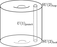
Figure 2: Mapping cylinder $\Sigma_{1,1}\times_{\varphi}I$. A global symmetry in the duality wall theory is associated to each component of boundary.

The mapping torus, $\textrm{tori}(\varphi):=\Sigma_{1,1}\times_{\varphi}S^{1}$, can be obtained by gluing the two boundary Riemann surfaces, $\Sigma^{\textrm{top}}_{1,1}$ and $\Sigma^{\textrm{bot}}_{1,1}$. In the duality wall theory, the gluing amounts to gauging the diagonal subgroup of the two $SU(2)$ global symmetries. The theory obtained by gluing two $SU(2)$’s in a duality wall theory $T[SU(2),\varphi]$ will be denoted as ${\rm Tr}(T[SU(2),\varphi])$. From the above discussion, we found a concrete realization of $T_{M}$ with $M=\textrm{tori}(\varphi)$ in terms of the duality wall theory. The theory will be denoted as $T^{T[SU(2)]}_{\textrm{tori}(\varphi)}$ ,

$$T^{T[SU(2)]}_{\textrm{tori}(\varphi)}={\rm Tr}(T[SU(2),\varphi])\;.$$ (6)

2.2 Tetrahedron decomposition

In Dimofte:2011ju , Dimofte, Gaiotto, Gukov (DGG) proposed a powerful algorithm to construct $T_{M}$ for a broad class of 3-manifolds $M$. We briefly review the DGG algorithm here. The basic building block of a hyperbolic 3-manifold is the ideal tetrahedron $\Delta$. The corresponding 3d theory, $T_{\Delta}$, is a theory of a free chiral field with a background CS action with level $-\frac{1}{2}$. If a 3-manifold $M$ can be triangulated by a finite number of tetrahedra, $T_{M}$ can be obtained by “gluing” copies of $T_{\Delta}$ accordingly. Schematically,

$$M=\left(\bigcup_{i=1}^{N}\Delta_{i}\right)/\sim\quad\Rightarrow\quad T_{M}=\left(\bigotimes_{i=1}^{N}T_{\Delta_{i}}\right)/\sim\;.$$ (7)

Geometry of tetrahedra

An ideal tetrahedron has six edges and four vertices. To the three pairs of diagonally opposite edges, we assign edge parameters $(z,z^{\prime},z^{\prime\prime})$ which are the exponential of complexified dihedral angles $(Z,Z^{\prime},Z^{\prime\prime})$ of the edges.

$$z=\exp(Z)\;\;\textrm{with}\;\;Z=(\textrm{torsion})+i(\textrm{angle})\,,\quad{\rm etc.}$$ (8)

Using the equivalence between equation of motion for hyperbolic metrics and $SL(2)$ flat connections on a 3-manifold, these edge variables can be understood in terms of either hyperbolic structure or $SL(2)$ flat connection on a tetrahedron. Although latter interpretation is more physically relevant, the former is more geometrically intuitive. The hyperbolic structure of an ideal tetrahedron is determined by the edge parameters $(Z,Z^{\prime},Z^{\prime\prime})$ subject to the conditions

$$Z+Z^{\prime}+Z^{\prime\prime}=\pi i+\frac{\hbar}{2}\,,\quad e^{Z}+e^{-Z^{\prime}}-1=0\,.$$ (9)

The first condition defines the so-called boundary phase space with the symplectic form $\Omega=\frac{1}{i\hbar}dZ\wedge dZ^{\prime}$. The second condition defines a Lagrangian submanifold of the boundary phase space. Due to the first condition, the second condition is invariant under the cyclic permutation $(z\rightarrow z^{\prime}\rightarrow z^{\prime\prime}\rightarrow z)$.

The ideal triangulation requires that all faces and edges of the tetrahedra should be glued such that the resulting manifold is smooth everywhere except for the cusp due to the vertices of ideal tetrahedra. In particular, we have the smoothness condition at each internal edge,

$$C_{I}=\sum_{j=1}^{N}\left(c_{Ij}Z_{i}+c^{\prime}_{Ij}Z^{\prime}_{j}+c^{\prime\prime}_{Ij}Z^{\prime\prime}_{j}\right)=2\pi i+\hbar\,.$$ (10)

The coefficients $c_{Ij}$, $c^{\prime}_{Ij}$, $c^{\prime\prime}_{Ij}$ take values in $\{0,1,2\}$.

When all the edges of $\Delta_{i}$ are glued, all but one of the gluing condition (10) give independent constraints, since the sum of all constraints, $\sum_{I}C_{I}=(2\pi i+\hbar)N$ trivially follows from $Z_{i}+Z^{\prime}_{i}+Z^{\prime\prime}_{i}=\pi i+\frac{\hbar}{2}$. The resulting manifold $M$ has a cusp boundary, composed of the truncated ideal vertices, which is topologically a torus $\mathbb{T}^{2}$. The two cycles of the torus, ‘longitude’ and ‘meridian’, describe the boundary phase space of $M$. The logarithmic variables for the two cycles, $V=\log(\ell)$ and $U=\log m$, are some linear combinations of $(Z_{i},Z^{\prime}_{i},Z^{\prime\prime}_{i})$.

Ideal triangulation of the mapping torus

The mapping torus $\textrm{tori}(\varphi)=\Sigma_{1,1}\times_{\varphi}S^{1}$ is known to be hyperbolic when $|\textrm{Tr}(\varphi)|>2$. The tetrahedron decomposition of these mapping torus is given explicitly in Gueritaud . Any $\varphi\in SL(2,\mathbb{Z})$ satisfying $|\textrm{Tr}(\varphi)|>2$ admits a unique decomposition of the following form,

$$\varphi=F\left(\varphi_{N}\varphi_{N-1}\ldots\varphi_{2}\varphi_{1}\right)F^{-1}\,,\quad\varphi_{i}=L\textrm{ or }R\;.$$ (11)

where we use the following convention for the $SL(2,\mathbb{Z})$ generators,

$$L=\begin{pmatrix}1&1\\ 0&1\end{pmatrix}\,,\;\;R=\begin{pmatrix}1&0\\ 1&1\end{pmatrix}=T\,,\;\;S=\begin{pmatrix}0&-1\\ 1&0\end{pmatrix}\,;\;\;L=S^{-1}T^{-1}S\,,\;\;S=L^{-1}RL^{-1}\,.$$ (12)

The overall conjugation by $F$ is immaterial in the definition of the mapping torus and can be neglected.

According to Gueritaud , to each letter $L$ or $R$ appearing in (11) one can associate a tetrahedron with edge parameters $(Z_{i},Z^{\prime}_{i},Z^{\prime\prime}_{i})$, or equivalently, $(z_{i},z^{\prime}_{i},z^{\prime\prime}_{i})=(e^{Z_{i}},e^{Z^{\prime}_{i}},e^{Z^{\prime\prime}_{i}})$. The index $i$ runs from 1 to $N$ with cyclic identification, $N+1\sim 1$. $L$ and $R$ generate ‘flips’ on the triangulation of $\Sigma_{1,1}$. Each flip corresponds to a tetrahedron (see figure 2 in Gueritaud ). There are $N$ tetrahedra in total and $3N$ edge parameters. In the mapping torus, all the edges of tetrahedra are glued and there are $N-1$ independent internal edge conditions. How the internal edges are glued together is determined by the decomposition (11) of $\varphi$. Taking account of the $N$ equations $Z_{i}+Z^{\prime}_{i}+Z^{\prime\prime}_{i}=i\pi+\frac{\hbar}{2}$ for each $i$, there are in total $2N-1$ linear constraints on $3N$ edge parameters. These $2N-1$ constraints can be solved by parameterizing $3N$ edge parameters by $N+1$ variables ($W_{i},V$) as shown in (13).

$$\begin{array}[]{c|cccc}\;\varphi_{i}\varphi_{i-1}&Z_{i}&Z^{\prime}_{i}&Z^{\prime\prime}_{i}&U_{i}\\[5.0pt] \hline\cr\\[-10.0pt] LL&\;i\pi+\frac{\hbar}{2}-W_{i}&\;W_{i}-\displaystyle{\frac{W_{i-1}+W_{i+1}}{2}}&\;\displaystyle{\frac{W_{i-1}+W_{i+1}}{2}}&\;0\\[15.0pt] RR&\;i\pi+\frac{\hbar}{2}-W_{i}&\;\displaystyle{\frac{W_{i-1}+W_{i+1}}{2}}&\;W_{i}-\displaystyle{\frac{W_{i-1}+W_{i+1}}{2}}&\;0\\[15.0pt] LR&\;i\pi+\frac{\hbar}{2}-W_{i}&\;\displaystyle{\frac{W_{i}+W_{i-1}-W_{i+1}-V-\pi i}{2}}&\;\displaystyle{\frac{W_{i}-W_{i-1}+W_{i+1}+V+\pi i}{2}}&\;-\displaystyle{\frac{W_{i}}{2}}\\[15.0pt] RL&\;i\pi+\frac{\hbar}{2}-W_{i}&\;\displaystyle{\frac{W_{i}-W_{i-1}+W_{i+1}+V+\pi i}{2}}&\;\displaystyle{\frac{W_{i}+W_{i-1}-W_{i+1}-V-\pi i}{2}}&\;+\displaystyle{\frac{W_{i}}{2}}\\[10.0pt] \end{array}$$ (13)

The particular form of the linear combination depends on the ordering of letters in (11). The reparametrization is ‘local’ in the sense that the expressions for $(Z_{i},Z^{\prime}_{i},Z^{\prime\prime}_{i})$ involve $W_{i}$ and $W_{i\pm 1}$ only. Among the remaining $N+1$ variables, as was explained below eq. (10), two are identified as ‘longitude’ and ‘meridian’. In (13), $\ell=e^{V}$ is the longitude variable, while the meridian variable $m=e^{U}$ is the product of all $m_{i}=e^{U_{i}}$, $U=\sum U_{i}$. As an example, tetrahedron decomposition of a mapping torus with $\varphi=LR$ is given in figure 3. In the case $\varphi=LR$, it is known that the mapping torus becomes the figure eight knot complement in $S^{3}$.

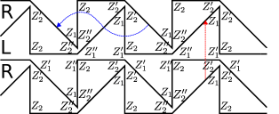
Figure 3: Triangulation of boundary torus of tori($LR$). Four triangles for each letter, $L$ or $R$, come from ‘small’ boundary triangles in ideal tetrahedron associated to the letter. See figure 3 in Gueritaud .

From the figure, the two internal edges are identified as

$$C_{1}=Z_{1}+Z_{2}+2Z^{\prime\prime}_{1}+2Z^{\prime\prime}_{2}=2\pi i+\hbar\;,$$

$$C_{2}=Z_{1}+Z_{2}+2Z_{1}^{\prime}+2Z_{2}^{\prime}=2\pi i+\hbar\;.$$ (14)

Longitudinal (horizontal blue line) and meridian (vertical red line) variables from the figure are

$$V=Z_{2}^{\prime\prime}-Z_{2}^{\prime}\;,\quad U=Z_{1}^{\prime\prime}-Z_{2}^{\prime}\;.$$ (15)

Using (13), we will parameterize

$$Z_{1}=i\pi+\frac{\hbar}{2}-W_{1}\;,\;Z_{1}^{\prime}=\frac{W_{1}+V+i\pi}{2}\;,\;Z_{1}^{\prime\prime}=\frac{W_{1}-V-i\pi}{2}\;,$$

$$Z_{2}=i\pi+\frac{\hbar}{2}-W_{2}\;,\;Z_{2}^{\prime}=\frac{W_{2}-V-i\pi}{2}\;,\;Z_{2}^{\prime\prime}=\frac{W_{1}+V+i\pi}{2}\;.$$

In this parametrization, the internal edge conditions (14) are automatically satisfied. From (13), the meridian variable $U$ is $\frac{W_{1}-W_{2}}{2}$ which is the same as the meridian variable in (15) via the above parametrization. But the longitudinal variable $V$ in (15) become $V+i\pi$ via the parametrization. The discrepancy $i\pi$ is subtle and the factor can be absorbed by simple redefinition of $V$ in (13). As we will see in section 4, however, the variable $V$ in (13) has a more direct meaning in the duality wall theory.

Field Theory

We will give a very brief summary of the construction of $T_{M,\Pi}$ from the tetrahedron decomposition data for $M$; see Dimofte:2011ju ; Dimofte:2011py for details. For each tetrahedron with a polarization choice $\Pi_{\Delta}$, we take a copy of the 3d theory $T_{\Delta,\Pi_{\Delta}}$. For the polarization $\Pi_{\Delta}=\Pi_{Z}$ in which we take $(Z,Z^{\prime\prime})$ as (position, momentum), the theory (often called “the tetrahedron theory”) is a free $\mathcal{N}=2$ chiral theory with a background CS term for the $U(1)$ global symmetry at CS level $-\frac{1}{2}$. The 3d theory $T_{M,\Pi_{M}}$ associated a 3-manifold $M=\cup_{i=1}^{N}\Delta_{i}/\sim$ and its boundary polarization $\Pi_{M}$ can be constructed in three steps. First, we start with a direct product of $N$ tetrahedron theories,

$$T_{\{\Delta_{i}\},\{\Pi_{Z_{i}}\}}=\otimes_{i=1}^{N}T_{\Delta_{i},\Pi_{Z_{i}}}$$ (16)

Then, we perform a polarization transformation $\tilde{\Pi}=g\circ\{\Pi_{Z_{i}}\}$ such that all internal edges and positions in $\Pi_{M}$ become position variables in $\tilde{\Pi}$. In the field theory, the polarization transformation corresponds to an $Sp(2N,\mathbb{Z})$ action involving the $U(1)^{N}$ global symmetries in $T_{\{\Delta_{i}\},\{\Pi_{Z_{i}}\}}$.

$$T_{\{\Delta_{i}\},\tilde{\Pi}}=g\circ T_{\{\Delta_{i}\},\{\Pi_{Z_{i}}\}}\;.$$ (17)

Finally, we impose the internal edges conditions (10) by adding the superpotential ${\cal W}=\sum{\cal O}_{I}$ which breaks the global $\otimes_{I}U(1)_{I}$ symmetries of $T_{\{\Delta_{i}\},\tilde{\Pi}}$ associated to internal edges $C_{I}$. This completes the consturction of $T_{M,\Pi}$:

$$T_{M,\Pi_{M}} =T_{\{\Delta_{i}\},\tilde{\Pi}}\textrm{ with superpotentail }{\cal W}=\sum{\cal O}_{I}\;.$$ (18)

Applying this general algorithm to the case $M=\textrm{tori}(\varphi)$ using the tetrahedron decomposition data described above, we give a description for the mapping torus theory. We will denote the mapping torus theory by $T^{\Delta}_{\textrm{tori}(\varphi)}$.

3 Quantization of Chern-Simons theory on Riemann Surface

In this section, we will explain the classical phase space and its quantization that are relevant to a calculation of Chern-Simons (CS) partition function on a mapping torus/cylinder. Most parts of this section are reviews of known results but are included to make the paper self-contained. More details can be found, e.g., in Dimofte:2011gm ; Dimofte:2011jd .

For a compact gauge group $G$, the Chern-Simons action on a 3-manifold $M$ is

$$I_{CS}=\frac{k}{4\pi}\int_{M}{\rm Tr}(A\wedge dA+\frac{2}{3}A\wedge A\wedge A)\;,$$ (19)

where $k$ is a quantized CS level. This is one of the most famous example of topological quantum field theory (TQFT). When $M$ is a mapping torus, the CS theory can be canonically quantized on $\Sigma_{1,1}$ regarding the $S^{1}$ direction as time. The phase space $\mathcal{M}_{G}$ canonically associated to $\Sigma_{1,1}$ is Elitzur:1989

$$\mathcal{M}_{G}(\Sigma_{1,1})=\{\textrm{Flat $G$-connections on $\Sigma_{1,1}$ with fixed puncture holonomy $P$}\}/\sim\;.$$ (20)

where $\sim$ denotes the gauge equivalence. The conjugacy class of gauge holonomy $P$ around a puncture is fixed as a boundary condition. The symplectic form $\Omega_{G}$ on ${\cal M}_{G}$ derived from the CS action is

$$\Omega_{G}=\frac{k}{4\pi}\int_{\Sigma}\textrm{Tr}(\delta A\wedge\delta A)\;.$$ (21)

One can geometrically quantize the classical phase space and obtain a Hilbert-space $\mathcal{H}_{G}(\Sigma_{1,1})$. Following an axiom of general TQFTs (see, e.g., Atiyah:1988 ), the CS partition function on the mapping cylinder with gauge group $G$ can be computed as

$$Z_{\Sigma_{1,1}\times_{\varphi}I}(x_{\rm bot},x_{\rm top})=\langle x_{\rm bot}|\varphi|x_{\rm top}\rangle\;,$$ (22)

which depends on the boundary conditions $\big{(}x_{\rm bot},\varphi(x_{\rm top})\big{)}$ on two boundary $\Sigma_{1,1}$’s . The CS partition function on the mapping torus with gauge group $G$ can be computed as

$$Z_{\textrm{tori}(\varphi)}(G)=\textrm{Tr}(\varphi)\;\textrm{over ${\cal H}_{G}(\Sigma_{1,1})$}.$$ (23)

Here $\varphi$ is an operator acting on the Hilbert space ${\cal H}_{G}$ obtained from quantizing a mapping class group element $\varphi$ which generates a coordinate transformation on $\mathcal{M}_{G}$.

When the gauge group is $G=SL(2,\mathbb{C})$, the CS level becomes complex variables $t=k+is$ and $\tilde{t}=k-is$. $k$ should be an integer for consistency of the quantum theory and unitarity requires $s\in\mathbb{R}$ or $s\in i\mathbb{R}$ Witten:91 .

$$I_{CS}=\frac{t}{8\pi}\int_{M}{\rm Tr}(A\wedge dA+\frac{2}{3}A\wedge A\wedge A)+\frac{\tilde{t}}{8\pi}\int_{M}{\rm Tr}(\bar{A}\wedge d\bar{A}+\frac{2}{3}\bar{A}\wedge\bar{A}\wedge\bar{A})\;.$$ (24)

The induced symplectic form from the CS action is

$$\Omega_{SL(2,\mathbb{C})}=\frac{t}{8\pi}\int_{\Sigma}\textrm{Tr}(\delta A\wedge\delta A)+\frac{\tilde{t}}{8\pi}\int_{\Sigma}\textrm{Tr}(\delta\bar{A}\wedge\delta\bar{A})\;.$$ (25)

In Dimofte:2011py , the superconformal index $I_{T_{M}}$ for the theory $T_{M}$ was claimed to be equivalent to the $SL(2,\mathbb{C})$ CS partition function on $M$ with $t=-\tilde{t}=is\in i\mathbb{R}$.

$$I_{T_{M}}=Z_{M}(SL(2,\mathbb{C}))\;,\;\textrm{with $q:=e^{\hbar}:=e^{\frac{4\pi}{s}}$}\;.$$ (26)

Here, $q$ is a fugacity variable in the superconformal index to be explained in section 4. Using the above map, the symplectic form becomes

$$\Omega_{SL(2,\mathbb{C})}:=\frac{i}{2\hbar}\int_{\Sigma}\textrm{Tr}(\delta A\wedge\delta A)-\frac{i}{2\hbar}\int_{\Sigma}\textrm{Tr}(\delta\bar{A}\wedge\delta\bar{A})\;.$$ (27)

3.1 Classical phase space and its coordinates

In this subsection, we will review coordinate systems for the phase space $(\mathcal{M},\Omega)_{SL(2,\mathbb{C})}$ on once-punctured torus $\Sigma_{1,1}$ and the action of $\varphi\in SL(2,\mathbb{Z})$ on these coordinates. We also consider a phase space $({\cal M},\Omega)^{\rm knot}_{SL(2,\mathbb{C})}$ which is canonically associated to the cusp boundary $\mathbb{T}^{2}$ of mapping torus. For mapping cylinder, the boundary phase space is given by, at least locally, ${\cal M}(\Sigma_{1,1})^{2}\times{\cal M}^{\rm knot}$.

Loop coordinates

Generally speaking, the moduli space of flat connections on manifold $M$ with gauge group $G$ is parametrized by holonomy variables up to conjugation. In other words,

$${\cal M}_{G}(M)=\textrm{Hom}(\pi_{1}(M),G)/\textrm{conj}.$$ (28)

The fundamental group for $\Sigma_{1,1}$ is

$$\pi_{1}(\Sigma_{1,1})=\{A,B,P|ABA^{-1}B^{-1}=P\}\;.$$ (29)

Here $A,B$ are two cycles of the torus and $P$ denotes the loop around the puncture. Thus ${\cal M}_{SL(2,\mathbb{C})}(\Sigma_{1,1})$ is given by

$${\cal M}_{SL(2,\mathbb{C})}=\{A,B\in SL(2,\mathbb{C})|ABA^{-1}B^{-1}=P\}/\textrm{conj}\;.$$ (30)

Conjugacy class of the holonomy $P$ around the puncture is fixed by the following condition

$$\textrm{eigenvalues of $P$}=\{\ell,\ell^{-1}\}\;.$$ (31)

Loop coordinates $(W,H,D)$ on ${\cal M}_{SL(2,\mathbb{C})}$ are defined as trace of these holonomy variables

$$W={\rm Tr}(A)\;,\quad H={\rm Tr}(B)\;,\quad D={\rm Tr}(AB)\;.$$ (32)

They are not independent and subject to the follwoing constraint:

$$W^{2}+H^{2}+D^{2}-WHD+\ell+\ell^{-1}-2=0\;.$$ (33)

Anticipating close relations to gauge theory observables, we call the three loop coordinates Wilson loop ($W$), ‘t Hooft loop ($H$) and dyonic loop ($D$).

Shear coordinates

The shear coordinates $(\sqrt{t},\sqrt{t^{\prime}},\sqrt{t^{\prime\prime}})$ are associated to the three edges appearing in the ideal triangulation of $\Sigma_{1,1}$ depicted in Figure 4.

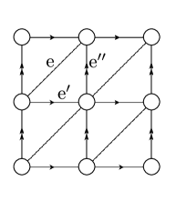
Figure 4: Triangulation of once-punctured torus, $\Sigma_{1,1}$, represented as $(\mathbb{R}^{2}-\mathbb{Z}^{2})/\mathbb{Z}^{2}$. Each circle in the figure denotes an image of the puncture in the covering space $\mathbb{R}^{2}$.

Naively, the shear coordinates represent the partial holonomy eigenvalues along a path crossing each edge. For more precise description of the shear coordinates, see, e.g., Fock:1993pr ; Fock:1997 . Following the description in the references, the holonomy $A,B$ can be expressed in terms of the shear coordinates as follows,

$$A(t,t^{\prime},t^{\prime\prime})={\cal E}(t){\cal V}{\cal E}^{-1}(t^{\prime}){\cal V}^{-1}=\left(\begin{array}[]{cc}\sqrt{tt^{\prime}}&\sqrt{tt^{\prime}}\\ \sqrt{\frac{t^{\prime}}{t}}&\frac{1}{\sqrt{tt^{\prime}}}+\sqrt{\frac{t^{\prime}}{t}}\end{array}\right)$$ (36)

$$B(t,t^{\prime},t^{\prime\prime})={\cal E}(t){\cal V}^{-1}{\cal E}^{-1}(t^{\prime\prime}){\cal V}=\left(\begin{array}[]{cc}\sqrt{\frac{t}{t^{\prime\prime}}}+\sqrt{tt^{\prime\prime}}&\sqrt{\frac{t}{t^{\prime\prime}}}\\ \frac{1}{\sqrt{tt^{\prime\prime}}}&\frac{1}{\sqrt{tt^{\prime\prime}}}\end{array}\right)\,,$$ (39)

where

$${\cal E}(z):=\left(\begin{array}[]{cc}0&z^{1/2}\\ -z^{-1/2}&0\end{array}\right)\;,\quad{\cal V}:=\left(\begin{array}[]{cc}1&1\\ -1&0\end{array}\right)\;.$$ (44)

The relation $ABA^{-1}B^{-1}=P$ in (30) holds provided that

$$\sqrt{t}\sqrt{t^{\prime}}\sqrt{t^{\prime\prime}}=\sqrt{-\ell}\;.$$ (45)

This relation states that products of partial holonomies around the three edges give the square root of holonomy around a puncture. The logarithmic shear variables $(T,T^{\prime},T^{\prime\prime})$ are defined as

$$(e^{T/2},e^{T^{\prime}/2},e^{T^{\prime\prime}/2})=(\sqrt{t},\sqrt{t^{\prime}},\sqrt{t^{\prime\prime}})\;.$$ (46)

Note that the matrices ($A,B$) in eq. (39) are invariant under individual shifts of $T,T^{\prime},T^{\prime\prime}$ by $4\pi i$.

$$T\sim T+4\pi i\;,\;T^{\prime}\sim T^{\prime}+4\pi i\;,\;T^{\prime\prime}\sim T^{\prime\prime}+4\pi i\;.$$ (47)

In the logarithmic variables, the condition (45) become

$$T+T^{\prime}+T^{\prime\prime}=i\pi+V\;.$$ (48)

From this, we see $V$ is also periodic variable with periodicity $4\pi i$. The symplectic form (27) takes a simple form in the shear coordinates.

$$\Omega_{SL(2,\mathbb{C})} =-\frac{i}{2\hbar}\frac{dt}{t}\wedge\frac{dt^{\prime}}{t^{\prime}}+\frac{i}{2\hbar}\frac{d\bar{t}}{\bar{t}}\wedge\frac{d\bar{t^{\prime}}}{\bar{t^{\prime}}}=-\frac{i}{2\hbar}dT\wedge dT^{\prime}+\frac{i}{2\hbar}d\bar{T}\wedge d\bar{T^{\prime}}$$

$$=(\textrm{cyclic permutation of }T\rightarrow T^{\prime}\rightarrow T^{\prime\prime})\;.$$ (49)

The $SL(2,\mathbb{Z})$ generators act on the shear coordinates as follows.

$$\begin{array}[]{c|ccc}\;\;\varphi&\sqrt{t}\mapsto&\sqrt{t^{\prime}}\mapsto&\;\;\sqrt{t^{\prime\prime}}\mapsto\\[5.0pt] \hline\cr\\[-10.0pt] \;\;S&\;\;\displaystyle{\frac{1}{\sqrt{t}}}&\;\;\displaystyle{\frac{\sqrt{t^{\prime\prime}}}{1+t^{-1}}}&\sqrt{t^{\prime}}(1+t)\\[12.0pt] \;\;L&\;\;\displaystyle{\frac{1}{\sqrt{t^{\prime\prime}}}}&\;\;\displaystyle{\frac{\sqrt{t^{\prime}}}{1+t^{\prime\prime-1}}}&\sqrt{t}(1+t^{\prime\prime})\\[12.0pt] \;\;R&\;\;\displaystyle{\frac{1}{\sqrt{t^{\prime}}}}&\;\;\displaystyle{\frac{\sqrt{t}}{1+t^{\prime-1}}}&\sqrt{t^{\prime\prime}}(1+t^{\prime})\end{array}$$ (50)

Fenchel-Nielson coordinates

We adopt the modified Fenchel-Nielson (FN) coordinates defined in Dimofte:2011jd . Classically, the FN coordinates $(\lambda,\tau):=(\exp\Lambda,\exp\mathcal{T})$ and the shear coordinates are related by

$$\sqrt{t}=\frac{i(\tau^{-1/2}-\tau^{1/2})}{\lambda-\lambda^{-1}}\,,\;\;\sqrt{t^{\prime}}=\frac{i(\lambda-\lambda^{-1})}{\lambda^{-1}\tau^{1/2}-\tau^{-1/2}\lambda}\,,\;\;\sqrt{t^{\prime\prime}}=\frac{i\sqrt{\ell}(\lambda^{-1}\tau^{1/2}-\tau^{-1/2}\lambda)}{\tau^{-1/2}-\tau^{1/2}}\,.$$ (51)

The FN coordinates are defined up to Weyl-reflection $\mathbb{Z}_{2}$, whose generator $\sigma$ acts as

$$\sigma\;:\;(\Lambda,\mathcal{T})\;\rightarrow\;(-\Lambda,-\mathcal{T})\;.$$ (52)

Note that the Weyl reflection leaves the shear coordinates invariant in the relation (51).

Phase space $({\cal M},\Omega)^{\textrm{knot}}_{SL(2,\mathbb{C})}$

So far we have considered a phase space associated to the Riemann surface $\Sigma_{1,1}$ in the $\textrm{tori}(\varphi)$. There is another important phase space in the computation of the CS partition function on $\textrm{tori}(\varphi)$ which is associated to the cusp boundary $\mathbb{T}^{2}=\partial(\textrm{tori}(\varphi))$. We denote this phase space by ${\cal M}^{\textrm{knot}}_{SL(2,\mathbb{C})}:={\cal M}_{SL(2,\mathbb{C})}(\mathbb{T}^{2})$ and parametrize it by the (logarithmic) holonomy variables $(U,V)$ along the two cycles of $\mathbb{T}^{2}$. The symplectic form $\Omega^{\textrm{knot}}$ is given by

$$\Omega^{\textrm{knot}}_{SL(2,\mathbb{C})}=\frac{1}{i\hbar}dU\wedge dV-\frac{1}{i\hbar}d\bar{U}\wedge d\bar{V}\;.$$ (53)

Boundary phase space of mapping cylinder

The boundary is the genus two Riemann surface without puncture, $\partial(\Sigma_{1,1}\times_{\varphi}I)=\Sigma_{2,0}$, which can be obtained by gluing punctures in two once-punctured tori. The fundamental group for $\Sigma_{2,0}$ is

$$\pi_{1}(\Sigma_{2,0})=\{A_{1},B_{1},A_{2},B_{2}|A_{1}B_{1}A_{1}^{-1}B_{1}^{-1}A_{2}B_{2}A_{2}^{-1}B_{2}^{-1}=1\}\;.$$ (54)

The non-trivial cycles $(A_{i},B_{i})$s on $\Sigma_{2,0}$ are depicted in Figure 5.

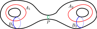
Figure 5: Generators of $\pi_{1}(\Sigma_{2,0})$

Thus, by eq. (28)

$$\mathcal{M}_{SL(2,\mathbb{C})}(\Sigma_{2,0})=\{A_{1},B_{1},A_{2},B_{2}\in SL(2,\mathbb{C})|A_{1}B_{1}A_{1}^{-1}B_{1}^{-1}A_{2}B_{2}A_{2}^{-1}B_{2}^{-1}=1\}/{\rm conj}\;.$$ (55)

The corresponding phase space ${\cal M}(\Sigma_{2,0})$ can be sliced by a constant $P:=A_{1}B_{1}A_{1}^{-1}B_{1}^{-1}=(A_{2}B_{2}A_{2}^{-1}B_{2}^{-1})^{-1}$ surface. In the slice, the phase space locally looks like a $GL(1,\mathbb{C})$ bundle of two copies of ${\cal M}(\Sigma_{1,1})$ with the same $\ell=e^{V}$, an eigenvalue of $P$. The $GL(1,\mathbb{C})$ fiber direction corresponds to opposite $GL(1,\mathbb{C})$ conjugation action on a representative elements $(A_{1},B_{1})$ and $(A_{2},B_{2})$ of the two ${\cal M}(\Sigma_{1,1})$’s, where the $GL(1,\mathbb{C})\subset SL(2,\mathbb{C})$ is the stabilizer subgroup of $P$. Locally, the boundary phase space looks like ${\cal M}(\Sigma_{1,1})^{2}\times{\cal M}^{\rm knot}$ where ${\cal M}^{\rm knot}$ is parameterized by conjugacy class of $P$ (or equivalently $V$) and the $GL(1,\mathbb{C})$ fiber direction. In total, $\textrm{dim}_{\mathbb{C}}\left[{\cal M}_{SL(2,\mathbb{C})}\big{(}\partial(\Sigma_{1,1}\times_{\varphi}I)\big{)}\right]=6$. As is obvious from the construction of ${\cal M}\big{(}\partial(\Sigma_{1,1}\times_{\varphi}I)\big{)}$, the $V$ variable in ${\cal M}\big{(}\partial(\Sigma_{1,1}\times_{\varphi}I)\big{)}$ can be identified with the puncture variable $V$ in ${\cal M}(\Sigma_{1,1})$. Considering the procedure of gluing two boundary $\Sigma_{1,1}$ components in $\Sigma_{1,1}\times_{\varphi}I$ to form a mapping torus $\Sigma_{1,1}\times_{\varphi}S^{1}$, the $V$ variable can also be identified with the longitudinal variable $V$ in ${\cal M}^{\rm knot}={\cal M}\big{(}\partial(\Sigma_{1,1}\times_{\varphi}S^{1})\big{)}$.

3.2 A-polynomial

Consider a 3-manifold $M$ with boundary $\partial M$. Obviously, the moduli space of $SL(2,\mathbb{C})$ flat connections on $M$ can be thought of as a submanifold of the moduli space on the boundary.

$${\cal M}(M)\subset{\cal M}(\partial M)\;.$$ (56)

In fact, the submanifold is Lagrangian with respect to the symplectic form (21). For a knot-complement $M$, the moduli space ${\cal M}(M)$ is $(\mathbb{C}^{*})^{2}/\mathbb{Z}_{2}$ parametrized by ‘longitude’ and ’meridian’ variable $(\ell,m)$ modulo a Weyl-reflection $(\ell,m)\sim(\ell^{-1},m^{-1})$. In this case the Lagrangian submanifold is given by the vanishing locus of the so-called “A-polynomial”, $A(\ell,m)$ Gukov:2003na . Mapping torus is one example of knot-complement. In this section we will analyze the A-polynomial for mapping torus from two different approaches and show their equivalence.

From tetrahedron decomposition

In (13), we presented a solution to the gluing conditions for the mapping torus by parametrizing the $3N$ edge parameters $(Z_{i},Z^{\prime}_{i},Z^{\prime\prime}_{i})$ for the $N$ tetrahedra in terms of $N+1$ parameters ($W_{i},V$). The A-polynomial for the mapping torus can be obtained by imposing additional $N$ non-linear constraints, $e^{Z_{i}}+e^{-Z^{\prime}_{i}}-1=0$, and eliminating all $W_{i}$’s in favor of $\ell=e^{V}$ and $m=\prod e^{U_{i}}$.

For instance, consider the simplest example, $\varphi=LR$ ($\varphi_{2}=L,\varphi_{1}=R$). From (13), we find ($w_{i}:=e^{W_{i}}$)

$$z_{1}=-\frac{1}{w_{1}}\,,\quad z^{\prime}_{1}=\sqrt{w_{1}(-\ell)}\,,\quad z^{\prime\prime}_{1}=\sqrt{\frac{w_{1}}{(-\ell)}}\,,$$

$$z_{2}=-\frac{1}{w_{2}}\,,\quad z^{\prime}_{2}=\sqrt{\frac{w_{2}}{(-\ell)}}\,,\quad z^{\prime\prime}_{2}=\sqrt{w_{2}(-\ell)}\,,\qquad m=\sqrt{\frac{w_{2}}{w_{1}}}\,.$$ (57)

For the boundary phase spaces of the two tetrahedra, the equations for the Lagrangian submanifolds ($z^{\prime}+(z^{\prime\prime})^{-1}-1=0$) are

$$\sqrt{w_{1}(-\ell)}+\sqrt{\frac{(-\ell)}{w_{1}}}-1=0\,,\quad\sqrt{\frac{w_{2}}{(-\ell)}}+\frac{1}{\sqrt{w_{2}(-\ell)}}-1=0\;.$$ (58)

Eliminating $w_{1}$ and $w_{2}$ in favor of $\ell$ and $m$, we obtain the A-polynomial for the mapping torus with $\varphi=LR$:

$$A(\ell,m)=\ell+\ell^{-1}-(m^{-2}-m^{-1}-2-m+m^{2})=0\;,$$ (59)

which coincide with A-polynomial for figure eight knot complement; see Gukov:2003na .

From Lagrangian submanifold for mapping cylinder

The Lagrangian submanifold for a mapping torus is a ‘diagonal’ subspace of a Lagrangian submanifold for the corresponding mapping cylinder Dimofte:2011jd . As explained above, the boundary phase space for the mapping cylinder contains a product of two phase spaces associated with two $\Sigma_{1,1}$’s at the two ends of the interval $I$,

$$\mathcal{M}^{\textrm{bot}}(\Sigma_{1,1})\times\mathcal{M}^{\textrm{top}}(\Sigma_{1,1})\subset{\cal M}\big{(}\partial(\Sigma_{1,1}\times_{\varphi}I)\big{)}\;,$$ (60)

where we labelled the two Riemann surface at the two ends of the interval $I$ by ‘top’ and ‘bot’(bottom). The phase space ${\cal M}^{\textrm{bot,top}}$ can be parametrized by two copies of shear coordinates $(t,t^{\prime},t^{\prime\prime})_{\textrm{bot,top}}$ with common $\ell$. The Lagrangian submanifold ${\cal L}_{\varphi}$ for mapping cylinder is Dimofte:2011jd

$${\cal L}_{\varphi}=\{t_{\textrm{top}}-\varphi_{*}(t)_{\textrm{bot}}=0,t^{\prime}_{\textrm{top}}-\varphi_{*}(t^{\prime})_{\textrm{bot}}=0,t^{\prime\prime}_{\textrm{top}}-\varphi_{*}(t^{\prime\prime})_{\textrm{bot}}=0\}\subset\mathcal{M}^{\textrm{bot}}\times\mathcal{M}^{\textrm{top}}\;.$$ (61)

Here $\varphi_{*}(O)$ is a coordinate for ${\cal M}_{SL(2,\mathbb{C})}$ which is related to $O$ by a mapping class group element $\varphi\in SL(2,\mathbb{Z})$. For example, $\varphi_{*}(t)=1/t^{\prime\prime}$ when $\varphi=L$ as one can see in (50). Among three equations between braces, only two equations are independent and the remaining one is automatically satisfied due to the relation $tt^{\prime}t^{\prime\prime}=-\ell$. Then, the Lagrangian submanifold for mapping torus is

$${\cal M}(\textrm{tori}(\varphi))={\cal L}_{1}\cap{\cal L}_{\varphi}\;.$$ (62)

${\cal L}_{1}$ denotes a diagonal subspace of $\mathcal{M}^{\textrm{bot}}\times\mathcal{M}^{\textrm{top}}$ which can be interpreted as the Langrangian submanifold for mapping cylinder with $\varphi=1$; see eq. (61).

However, the above construction for the Langrangian submanifold of $\textrm{tori}(\varphi)$ is incomplete since all the algebraic equations depend on $\ell$ but not on $m$. We need an additional algebraic relation involving $m$. As we saw above, $U=\log m$ is conjugate to $V=\log\ell$. Anticipating the consequences of quantization, which promotes $m$ to a shift operator ($m:\ell\rightarrow q\ell$), we propose the following prescription for $m$; see (96).

$$m=1\;,\quad\textrm{for $\varphi=R$}$$

$$m=\frac{\sqrt{t}_{\textrm{top}}}{\sqrt{t}_{\textrm{bot}}}\;,\quad\textrm{for $\varphi=L$}\;.$$ (63)

Consider general $\varphi$ which can be written as product of $L$ and $R$,

$$\varphi=\varphi_{N}\cdots\varphi_{1}\;,\quad\varphi_{i}=L\textrm{ or }R\;.$$ (64)

For each letter $\varphi_{i}$, we assign a mapping cylinder $\Sigma_{1,1}\times_{\varphi_{i}}I$ whose boundary phase space associated to two boundary $\Sigma_{1,1}$’s is parameterized by $(t_{i},t^{\prime}_{i},t^{\prime\prime}_{i})_{\textrm{bot},\textrm{top}}$. To glue $\Sigma^{\textrm{bot}}_{1,1}$ of $i$-th mapping cylinder with $\Sigma^{\textrm{top}}_{1,1}$ of $i+1$-th mapping cylinder, we parametrize

$$(t_{i},t^{\prime}_{i},t^{\prime\prime}_{i})_{\textrm{bot}}=(t_{i+1},t^{\prime}_{i+1},t^{\prime\prime}_{i+1})_{\textrm{top}}:=(t_{i+1},t_{i+1}^{\prime},t_{i+1}^{\prime\prime})\;.$$ (65)

$i$ is a cyclic parameter running from 1 to $N$, $N+1\sim 1$. In the parametrization, the Lagrangian in (61) becomes

$${\cal L}_{\varphi_{i}}(t^{*}_{i},t^{*}_{i+1})=\left\{\begin{array}[]{ll}\{\sqrt{t_{i}}-\frac{1}{\sqrt{t^{\prime\prime}_{i+1}}}=0,\;\sqrt{t^{\prime\prime}_{i}}-\sqrt{t_{i+1}}(1+t^{\prime\prime}_{i+1})=0\}\;,&\quad\varphi_{i}=L\\ \{\sqrt{t_{i}}-\frac{1}{\sqrt{t^{\prime}_{i+1}}}=0,\;\sqrt{t^{\prime}_{i}}-\sqrt{t_{i+1}}/(1+1/t^{\prime}_{i+1})=0\}\;,&\quad\varphi_{i}=R\end{array}\right.$$ (68)

Equation involving $m$ for mapping cylinder $\Sigma_{1,1}\times_{\varphi}I$ is

$$m=\prod_{i=1}^{N}m_{i}\;,\quad\textrm{where}$$

$$m_{i}=\left\{\begin{array}[]{ll}1\;,&\quad\textrm{$\varphi_{i}$ = R}\\ \frac{\sqrt{t_{i}}}{\sqrt{t_{i+1}}}\;,&\quad\textrm{$\varphi_{i}$ = L}\end{array}\right.$$ (71)

Since $m$ act as a shift operator, $m$ for $\varphi_{N}\ldots\varphi_{1}$ is product of $m_{i}$ for each $\varphi_{i}$. Then, the A-polynomial for tori($\varphi$) is given by solving all equations in (68),(71) in terms of $(\ell,m)$.

Equivalence of two approaches

In the above, we explained two ways of calculating the A-polynomial for the mapping torus. The equivalence of the two approaches can be explicitly shown by i) finding a map between $(w_{i})$ variables in the first approach and $(t^{*}_{i})$ variables in the second approach and ii) showing that the equations (68), (71) in the second approach are either trivially satisfied or mapped into equations in the first approach. The map we found is

$$\begin{array}[]{c|ccc}\;\;\varphi_{i-1}&t_{i}&t^{\prime}_{i}&t^{\prime\prime}_{i}\\[5.0pt] \hline\cr\\[-10.0pt] \;L&\;\;\;\displaystyle{\frac{1}{w_{i}}}&\;(-\ell)\displaystyle{\frac{w_{i}}{w_{i-1}}}&\;w_{i-1}\\[12.0pt] \;R&\;\;\;\displaystyle{\frac{1}{w_{i}}}&\;w_{i-1}&\;(-\ell)\displaystyle{\frac{w_{i}}{w_{i-1}}}\end{array}$$ (72)

From the fact that a single flip ($\varphi_{i-1}$ =$L$ or $R$) generate a tetrahedron whose edges are originated from edges in a triangulation of $\Sigma_{1,1}$, identification of $\frac{1}{w_{i}}$ (which is $-z_{i}$) with $t_{i}$ is understandable. For $\varphi_{i}=L$, the map (72) ensures that the transformation rule $\sqrt{t_{i}}=1/\sqrt{t^{\prime\prime}_{i+1}}$ in (68) is trivially satisfied. The other transformation rule, $\sqrt{t^{\prime\prime}_{i}}=\sqrt{t_{i+1}}(1+t_{i+1}^{\prime\prime})$, is equivalent to the constraint $z^{\prime\prime}_{i}+(z_{i})^{-1}-1=0$. Similarly, for $\varphi_{i}=R$, the transformation rule $\sqrt{t_{i}}=1/\sqrt{t^{\prime}_{i+1}}$ in (68) is trivially satisfied, while $\sqrt{t^{\prime}_{i}}=\sqrt{t_{i+1}}/(1+1/t^{\prime}_{i+1})$ is equivalent to $z^{\prime\prime}_{i}+(z_{i})^{-1}-1=0$. Finally, we note that the meridian variable $m$ can be written in terms of the shear coordinates as

$$m=\frac{\prod_{\varphi_{i}\varphi_{i-1}=RL}\sqrt{w_{i}}}{\prod_{\varphi_{i}\varphi_{i-1}=LR}\sqrt{w_{i}}} =\prod_{\varphi_{i}=L}\frac{\sqrt{w_{i+1}}}{\sqrt{w_{i}}}=\prod_{\varphi_{i}=L}\frac{\sqrt{t_{i}}}{\sqrt{t_{i+1}}}\;,$$ (73)

which is the same as the last equation in (71).

Thus we have proved the classical equivalence of the two approaches using the A-polynomial. This classical equivalence was already observed in Terashima:2011xe . In section 4.4.1, we will prove the equivalence at the quantum level by computing the $SL(2,\mathbb{C})$ CS partition function from the two approaches and confirming an exact agreement. The quantized $(\ell,m)$ variables, denoted as ($\mathfrak{l},\mathfrak{m}$), act as difference operators on the CS partition function. The quantum A-polynomial $A(\mathfrak{l},\mathfrak{m};q)$ annihilates the CS partition function. Taking the classical limit, $q\rightarrow 1$, we obtain the A-polynomial, $A(\ell,m)$ discussed in this section.

3.3 Quantization for $G=SL(2,\mathbb{C})$

In this section, we will quantize the classical phase spaces $(\mathcal{M},\Omega)_{SL(2,\mathbb{C})}$ and $(\mathcal{M},\Omega)^{\rm knot}_{SL(2,\mathbb{C})}$. By quantization of the classical phase space $(\mathcal{M},\Omega)$, we mean finding the following maps:

$$\textrm{Classical phase space }\mathcal{M}\quad\rightarrow\quad\textrm{Hilbert-space }{\cal H}$$

$$\textrm{Observables (functions of coordinate $x_{i}$) $O(x_{i})$ }\quad\rightarrow\quad\textrm{Operators $\mathsf{O}(\mathsf{x}_{i})$ acting on }{\cal H}$$

$$\textrm{Poisson bracket $\{O_{1},O_{2}\}=O_{3}$}\quad\rightarrow\quad\textrm{Commutation relation $[\mathsf{O}_{1},\mathsf{O}_{2}]=\mathsf{O}_{3}$}\;.$$ (74)

The two main ingredients of quantization are the Hilbert-space ${\cal H}$ and operators $\{\mathsf{O}\}$ acting on it. In this section, we will focus on the latter. Operators and their commutation relations can be considered before constructing a concrete Hilbert-space. The construction of the Hilbert-space will be given in section 4 .

Extended shear operators

After quantization, the shear coordinates $T,T^{\prime},T^{\prime\prime}$ (and its conjugations) become operators

$$(T,T^{\prime},T^{\prime\prime})\rightarrow(\mathsf{T}_{+},\mathsf{T}^{\prime}_{+},\mathsf{T}^{\prime\prime}_{+})\;,$$

$$(\bar{T},\bar{T}^{\prime},\bar{T}^{\prime\prime})\rightarrow(\mathsf{T}_{-},\mathsf{T}^{\prime}_{-},\mathsf{T}^{\prime\prime}_{-})\;.$$ (75)

The commutation relations for these shear operators follow from the symplectic form (49),

$$[\mathsf{T}_{\pm},\mathsf{T}^{\prime}_{\pm}]=[\mathsf{T}^{\prime}_{\pm},\mathsf{T}^{\prime\prime}_{\pm}]=[\mathsf{T}^{\prime\prime}_{\pm},\mathsf{T}_{\pm}]=\pm 2\hbar\,.$$ (76)

$$[\mathsf{T}^{*}_{\pm},\mathsf{T}^{**}_{\mp}]=0\;,\quad\textrm{for any }*,**\;.$$ (77)

The exponentiated operators $(\sqrt{\mathsf{t}}=e^{\frac{1}{2}\mathsf{T}},\sqrt{\mathsf{t}^{\prime}}=e^{\frac{1}{2}\mathsf{T}^{\prime}},\sqrt{\mathsf{t}^{\prime\prime}}=e^{\frac{1}{2}\mathsf{T}^{\prime\prime}})$ satisfy

$$\sqrt{\mathsf{t}}\sqrt{\mathsf{t}^{\prime}}=q^{\frac{1}{2}}\sqrt{\mathsf{t}^{\prime}}\sqrt{\mathsf{t}}\,,\quad\sqrt{\mathsf{t}^{\prime}}\sqrt{\mathsf{t}^{\prime\prime}}=q^{\frac{1}{2}}\sqrt{\mathsf{t}^{\prime\prime}}\sqrt{\mathsf{t}^{\prime}}\,,\quad\sqrt{\mathsf{t}^{\prime\prime}}\sqrt{\mathsf{t}^{\prime}}=q^{\frac{1}{2}}\sqrt{\mathsf{t}^{\prime}}\sqrt{\mathsf{t}^{\prime\prime}}\,.$$ (78)

Recall that the quantum parameter $q$ is defined as $q:=e^{\hbar}$. From here on, we will ignore the subscript $(\pm)$ and all expressions will be for $(+)$ operators unless otherwise stated. The same expressions hold for the $(-)$ operators upon replacing $q$ by $q^{-1}$.

Quantizing (45), shear operators are subject to the following central constraint.

$$\sqrt{\mathsf{t}}\sqrt{\mathsf{t}^{\prime}}\sqrt{\mathsf{t}^{\prime\prime}}=q^{\frac{1}{4}}\sqrt{-\ell}\;.$$ (79)

In the logarithmic shear operators, the constraint becomes

$$\mathsf{T}+\mathsf{T}^{\prime}+\mathsf{T}^{\prime\prime}=V+i\pi\;.$$ (80)

In the literature, the variable $V$ is usually regarded as a central charge since they are focusing on the Riemann surface $\Sigma_{1,1}$ itself where $V$ is a fixed parameter. But, when considering mapping cylinder or torus, we need to elevate $V$ to a quantum operator $\mathsf{V}$ and introduce its conjugate operator $\mathsf{U}$ satisfying

$$[\mathsf{U},\mathsf{V}]=\hbar\;,$$ (81)

since $V$ appears as a dynamical variable (a coordinate for the boundary phase space). Then, the central constraint is promoted to an operator relation

$$\mathsf{T}+\mathsf{T}^{\prime}+\mathsf{T}^{\prime\prime}=\mathsf{V}+i\pi\,.$$ (82)

Since $\mathsf{V}$ originates from the central constraint, it is natural to assume that

$$[\mathsf{V},\mathsf{T}]=[\mathsf{V},\mathsf{T}^{\prime}]=[\mathsf{V},\mathsf{T}^{\prime\prime}]=0\,.$$ (83)

We cannot require that $\mathsf{U}$ commute with all three shear coordinates; that would contradict with (81) and (82). The best we can do is to demand that $\mathsf{U}$ commutes with two of the shear coordinates and to determine the last commutator with (81) and (82). For instance,

$$[\mathsf{U},\mathsf{T}]=[\mathsf{U},\mathsf{T}^{\prime}]=0\quad\Longrightarrow\quad[\mathsf{U},\mathsf{T}^{\prime\prime}]=\hbar\,.$$ (84)

Alternatively, we may choose

$$[\mathsf{U}^{\prime},\mathsf{T}^{\prime}]=[\mathsf{U}^{\prime},\mathsf{T}^{\prime\prime}]=0\quad\Longrightarrow\quad[\mathsf{U}^{\prime},\mathsf{T}]=\hbar\,,$$

$$[\mathsf{U}^{\prime\prime},\mathsf{T}^{\prime\prime}]=[\mathsf{U}^{\prime\prime},\mathsf{T}]=0\quad\Longrightarrow\quad[\mathsf{U}^{\prime\prime},\mathsf{T}^{\prime}]=\hbar\,.$$ (85)

The three choices are related by simple canonical transformations,

$$\mathsf{U}^{\prime}=\mathsf{U}-\frac{1}{2}\mathsf{T}^{\prime}\,,\quad\mathsf{U}^{\prime\prime}=\mathsf{U}+\frac{1}{2}\mathsf{T}\,.$$ (86)

Among these choices, $\mathsf{U}$ (instead of $\mathsf{U}^{\prime},\mathsf{U}^{\prime\prime}$) is identified as quantum counterpart of the classical ‘meridian‘ variables $U$ in ${\cal M}^{\textrm{knot}}$. $\mathsf{V}$ is identified as a quantum counterpart of ‘longitudinal’ variable $\mathsf{V}$ in ${\cal M}^{\textrm{knot}}$.

Now, we can give a more precise meaning to the expression in (22), (23). If we consider $V$ as a fixed parameter, the trace of $\varphi$ will be a function on the parameter, $\textrm{Tr}(\varphi)(V)$. On the other hand, the CS partition function $Z_{\textrm{tori}}$ should be understood as a wave-function in the Hilbert space $\mathcal{H}^{\textrm{knot}}$ associated to a choice of polarization $\Pi=({\cal X},{\cal P})$,

$$Z_{\textrm{tori}(\varphi)}(x)=\;_{\Pi}\langle{\cal X}=x|Z_{\textrm{tori}(\varphi)}\rangle\;,\quad|Z_{\textrm{tori}(\varphi)}\rangle\in{\cal H}^{\textrm{knot}}\;.$$ (87)

Here ${}_{\Pi}\langle{\cal X}=x|$ denotes a position eigenstate in $\Pi$ polarization. A more precise statement of (23) is that the function $\textrm{Tr}(\varphi)(V)$ is a wave-function in the polarization $\Pi=(\mathsf{V},\mathsf{U})$:

$$\textrm{Tr}(\varphi)(V)=\;_{\Pi}\langle{\cal X}=V|Z_{\textrm{tori}(\varphi)}\rangle\;,$$ (88)

Using the quantum operator $\mathsf{V}$, the above can be written as (in the choice $\Pi=(\mathsf{V},\mathsf{U})$)

$$\textrm{Tr}(\varphi)(V) =\;_{\Pi}\langle{\cal X}=V|{\rm Tr}(\varphi)(\mathsf{V})|{\cal P}=0\rangle_{\Pi}$$

$$=\;_{\Pi}\langle{\cal X}=V|{\rm Tr}(\varphi)(\mathsf{V})|\mathsf{U}=0\rangle\;.$$ (89)

Thus, we find the following polarization-independent expression,

$$|Z_{\textrm{tori}(\varphi)}\rangle={\rm Tr}(\varphi)|\mathsf{U}=0\rangle\in{\cal H}^{\rm knot}\;.$$ (90)

Similarly, for mapping cylinder, the precise meaning of (22) is

$$|Z_{\Sigma_{1,1}\times_{\varphi}I}\rangle=\varphi|\mathsf{U}=0\rangle\in{\cal H}(\Sigma_{1,1})\otimes\overline{{\cal H}(\Sigma_{1,1})}\otimes{\cal H}^{\rm knot}\;.$$ (91)

Recall that the boundary phase space of mapping cylinder is locally ${\cal M}(\Sigma_{1,1})^{2}\times{\cal M}^{\rm knot}$ and quantization of the phase space gives a Hilbert-space ${\cal H}(\Sigma_{1,1})\otimes\overline{{\cal H}(\Sigma_{1,1})}\otimes{\cal H}^{\rm knot}$. $\overline{{\cal H}}$ denote a dual Hilbert-space and the structure ${\cal H}\otimes\overline{{\cal H}}$ is due to the two oppositely oriented boundary Riemann surfaces.

Since $(\sqrt{t},\sqrt{t^{\prime}},\sqrt{t^{\prime\prime}},\ell)$ and $(\sqrt{\bar{t}},\sqrt{\bar{t}^{\prime}},\sqrt{\bar{t}^{\prime\prime}},\bar{\ell})$ are related by complex conjugation, it is natural to define the adjoint of their quantum counterparts as follows

$$(\sqrt{\mathsf{t}},\sqrt{\mathsf{t}^{\prime}},\sqrt{\mathsf{t}^{\prime\prime}},\mathfrak{l}:=e^{\mathsf{V}})_{\pm}^{\dagger}=(\sqrt{\mathsf{t}},\sqrt{\mathsf{t}^{\prime}},\sqrt{\mathsf{t}^{\prime\prime}},\mathfrak{l})_{\mp}\;.$$ (92)

SL$(2,\mathbb{Z})$ action

Under the action of the generators of SL$(2,\mathbb{Z})$ in (12), the transformation rule for the quantum shear coordinates can be summarized as follows.

$$\begin{array}[]{c|ccc}\;\;\varphi&\sqrt{\mathsf{t}}\mapsto&\sqrt{\mathsf{t}^{\prime}}\mapsto&\;\;\sqrt{\mathsf{t}^{\prime\prime}}\mapsto\\[5.0pt] \hline\cr\\[-10.0pt] \;\;S&\;\;\displaystyle{\frac{1}{\sqrt{\mathsf{t}}}}&\;\;\sqrt{\mathsf{t}^{\prime\prime}}\displaystyle{\frac{1}{1+q^{\frac{1}{2}}\mathsf{t}^{-1}}}&\sqrt{\mathsf{t}^{\prime}}(1+q^{\frac{1}{2}}\mathsf{t})\\[12.0pt] \;\;L&\;\;\displaystyle{\frac{1}{\sqrt{\mathsf{t}^{\prime\prime}}}}&\;\;\sqrt{\mathsf{t}^{\prime}}\displaystyle{\frac{1}{1+q^{\frac{1}{2}}\mathsf{t}^{\prime\prime-1}}}&\sqrt{\mathsf{t}}(1+q^{\frac{1}{2}}\mathsf{t}^{\prime\prime})\\[12.0pt] \;\;R&\;\;\displaystyle{\frac{1}{\sqrt{\mathsf{t}^{\prime}}}}&\;\;\sqrt{\mathsf{t}}\displaystyle{\frac{1}{1+q^{\frac{1}{2}}\mathsf{t}^{\prime-1}}}&\sqrt{\mathsf{t}^{\prime\prime}}(1+q^{\frac{1}{2}}\mathsf{t}^{\prime})\end{array}$$ (93)

After quantization, the $SL(2,\mathbb{Z})$ transformation $\varphi$ becomes an operator acting on Hilbert-space. Operator $\varphi$ can be expressed in terms of $(\mathsf{T},\mathsf{T}^{\prime},\mathsf{T}^{\prime\prime})_{\pm}$. For $\varphi=\mathsf{L}$ and $\mathsf{R}$, the operator is determined by the following conditions

$$\mathsf{L}\cdot\sqrt{\mathsf{t}_{\pm}}=\frac{1}{\sqrt{\mathsf{t}^{\prime\prime}_{\pm}}}\cdot\mathsf{L}\;,\quad\mathsf{L}\cdot\sqrt{\mathsf{t}^{\prime\prime}_{\pm}}-\sqrt{\mathsf{t}_{\pm}}(1+q^{\pm 1/2}\mathsf{t}^{\prime\prime}_{\pm})\cdot\mathsf{L}=0\;,$$

$$\mathsf{R}\cdot\sqrt{\mathsf{t}_{\pm}}=\frac{1}{\sqrt{\mathsf{t}^{\prime}_{\pm}}}\cdot\mathsf{R}\;,\quad\mathsf{R}\cdot\sqrt{\mathsf{t}^{\prime\prime}_{\pm}}-\sqrt{\mathsf{t}^{\prime\prime}_{\pm}}(1+q^{\pm 1/2}\mathsf{t}^{\prime}_{\pm})\cdot\mathsf{R}=0\;.$$ (94)

The solution for the operator equation can be given as follows

$$\mathsf{L}=\mathsf{L}_{+}\mathsf{L}_{-}=\left(\prod_{r=1}^{\infty}\frac{1+q^{r-\frac{1}{2}}(\mathsf{t}^{\prime\prime}_{+})^{-1}}{1+q^{r-\frac{1}{2}}(\mathsf{t}^{\prime\prime}_{-})^{-1}}\right)\exp\left[-\frac{1}{4\hbar}\left((\mathsf{T}^{\prime\prime}_{+}+\mathsf{T}_{+})^{2}-(\mathsf{T}^{\prime\prime}_{-}+\mathsf{T}_{-})^{2}\right)\right]\;,$$

$$\mathsf{R}=\mathsf{R}_{+}\mathsf{R}_{-}=\left(\prod_{r=1}^{\infty}\frac{1+q^{r-\frac{1}{2}}\mathsf{t}^{\prime}_{-}}{1+q^{r-\frac{1}{2}}\mathsf{t}^{\prime}_{+}}\right)\exp\left[\frac{1}{4\hbar}\left((\mathsf{T}^{\prime}_{+}+\mathsf{T}_{+})^{2}-(\mathsf{T}^{\prime}_{-}+\mathsf{T}_{-})^{2}\right)\right]\;.$$ (95)

From the solution, we find that ($\mathfrak{m}:=e^{\mathsf{U}}$)

$$\mathfrak{m}_{\pm}\cdot\mathsf{L}\cdot\mathfrak{m}_{\pm}^{-1}=\frac{1}{\sqrt{\mathsf{t}_{\pm}}}\cdot\mathsf{L}\cdot\sqrt{\mathsf{t}_{\pm}}$$

$$\mathfrak{m}_{\pm}\cdot\mathsf{R}\cdot\mathfrak{m}_{\pm}^{-1}=\mathsf{R}\;.$$ (96)

We use that $\mathfrak{m}_{\pm}\cdot\mathsf{t}^{\prime\prime}_{\pm}\cdot\mathfrak{m}_{\pm}^{-1}=q^{\pm 1}\mathsf{t}^{\prime\prime}_{\pm}$. This give a derivation of (63). Note that these operators are all unitary; see (92). Since all $SL(2,\mathbb{Z})$ elements can be constructed by multiplying $\mathsf{L},\mathsf{R}$ and their inverses, we can easily see that all $\varphi\in SL(2,\mathbb{Z})$ are unitary operators. As we will see in section 4, this unitarity is closely related to $SL(2,\mathbb{Z})$ duality invariance of the supeconformal index for 4d $\mathcal{N}=2^{*}$ theory.

Shear vs Fenchel-Nielson

Quantization of the FN coordinates can be summarized as

$$\hat{\tau}=e^{\hat{\mathcal{T}}}\,,\;\;\hat{\lambda}=e^{\hat{\Lambda}}\,,\quad[\hat{\mathcal{T}},\hat{\Lambda}]=\hbar\,,\quad\hat{\tau}\hat{\lambda}=q\hat{\lambda}\hat{\tau}\,.$$ (97)

The relation to quantum shear coordinates was given in Dimofte:2011jd .

$$\sqrt{\mathsf{t}}=\frac{i}{\hat{\lambda}-\hat{\lambda}^{-1}}(\hat{\tau}^{-\frac{1}{2}}-\hat{\tau}^{\frac{1}{2}})\,,$$

$$\sqrt{\mathsf{t}^{\prime}}=\frac{i}{q^{-\frac{1}{4}}\hat{\lambda}^{-1}\hat{\tau}^{\frac{1}{2}}-q^{\frac{1}{4}}\hat{\tau}^{-\frac{1}{2}}\hat{\lambda}}(\hat{\lambda}-\hat{\lambda}^{-1})\,,$$

$$\sqrt{\mathsf{t}^{\prime\prime}}=\frac{iq^{\frac{1}{4}}\mathfrak{l}^{\frac{1}{2}}}{\hat{\tau}^{-\frac{1}{2}}-\hat{\tau}^{\frac{1}{2}}}(q^{-\frac{1}{4}}\hat{\lambda}^{-1}\hat{\tau}^{\frac{1}{2}}-q^{\frac{1}{4}}\hat{\tau}^{-\frac{1}{2}}\hat{\lambda})\,.$$ (98)

Loop vs Fenchel-Nielson

Quantizing the loop coordinates $(W,H,D)$ yields Dimofte:2011jd

$$\mathsf{W}=\hat{\lambda}+\hat{\lambda}^{-1}\;,$$

$$\mathsf{H}=\frac{q^{-\frac{1}{4}}\mathfrak{l}^{\frac{1}{2}}\hat{\lambda}-q^{\frac{1}{4}}\mathfrak{l}^{-\frac{1}{2}}\hat{\lambda}^{-1}}{\hat{\lambda}-\hat{\lambda}^{-1}}\hat{\tau}^{-\frac{1}{2}}+\frac{q^{\frac{1}{4}}\mathfrak{l}^{-\frac{1}{2}}\hat{\lambda}-q^{-\frac{1}{4}}\mathfrak{l}^{\frac{1}{2}}\hat{\lambda}^{-1}}{\hat{\lambda}-\hat{\lambda}^{-1}}\hat{\tau}^{\frac{1}{2}}\;.$$

$$\mathsf{D}=\frac{q^{-\frac{1}{4}}\mathfrak{l}^{\frac{1}{2}}\hat{\lambda}-q^{\frac{1}{4}}\mathfrak{l}^{-\frac{1}{2}}\hat{\lambda}^{-1}}{\hat{\lambda}-\hat{\lambda}^{-1}}q^{-\frac{1}{4}}\hat{\lambda}\hat{\tau}^{-\frac{1}{2}}+\frac{q^{\frac{1}{4}}\mathfrak{l}^{-\frac{1}{2}}\hat{\lambda}-q^{-\frac{1}{4}}\mathfrak{l}^{\frac{1}{2}}\hat{\lambda}^{-1}}{\hat{\lambda}-\hat{\lambda}^{-1}}q^{-\frac{1}{4}}\hat{\lambda}^{-1}\hat{\tau}^{\frac{1}{2}}\;.$$ (99)

4 Superconformal index/$SL(2,\mathbb{C})$ CS partition function

The superconformal index for 3d SCFTs with global symmetry $U(1)^{N}$ is defined as Kim:2009wb ; Imamura:2011su ; Krattenthaler:2011da ; Kapustin:2011jm

$$I(q,m_{i},u_{i})=\textrm{Tr}(-1)^{F}q^{\frac{1}{2}R+j_{3}}\prod_{i=1}^{N}u_{i}^{H_{i}}$$ (100)

where the trace is taken over Hilbert-space $\mathcal{H}_{\{m_{i}\}}$ on $S^{2}$, where background monopole fluxes $\{m_{i}\}$ coupled to global symmetries $U(1)^{N}$ are turned on. $R$ and $j_{3}$ denote $U(1)$ R-charge and spin on $S^{2}$ respectively. $\{u_{i}\}$ are fugacity variables for the $U(1)^{N}$ whose generators are denoted by $\{H_{i}\}$. It is often useful to express the index in a charge basis $(m_{i},e_{i})$ instead of $(m_{i},u_{i})$,

$$I(m_{i},u_{i})=\sum_{e_{i}}I(m_{i},e_{i})u_{i}^{e_{i}}\;.$$ (101)

In the charge basis, the $Sp(2N,\mathbb{Z})$ transformation Witten:2003ya on 3d SCFTs with $U(1)^{N}$ global symmetry acts linearly. For two 3d SCFTs, $\mathcal{T}$ and $g\cdot\mathcal{T}$, related by $g\in Sp(2N,\mathbb{Z})$, the generalized indices for the two theories are related as Dimofte:2011py

$$I_{g\cdot\mathcal{T}}(m,e)=I_{\mathcal{T}}(g^{-1}\cdot(m,e))\;.$$ (102)

In section 2, we gave two alternative descriptions for mapping torus theories which we denote by $T^{\textrm{T[SU(2)]}}_{\textrm{tori}(\varphi)}$ and $T^{\Delta}_{\textrm{tori}(\varphi)}$. The two descriptions give seemingly different expressions for the index. We will denote the index for $T^{\textrm{T[SU(2)]}}_{\textrm{tori}(\varphi)}$ and $T^{\Delta}_{\textrm{tori}(\varphi)}$ by $I^{\textrm{T[SU(2)]}}_{\textrm{tori}(\varphi)}$ and $I^{\Delta}_{\textrm{tori}(\varphi)}$, respectively. By proving

$$I^{\textrm{T[SU(2)]}}_{\textrm{tori}(\varphi)}=I^{\Delta}_{\textrm{tori}(\varphi)}$$ (103)

for general $\varphi$ with $|{\rm Tr}(\varphi)|>2$, we will confirm the equivalence of two descriptions at the quantum level. The 3d-3d correspondence Dimofte:2011py predicts that the index is the same as the $SL(2,\mathbb{C})$ CS partition function on the mapping torus, $Z_{\textrm{tori}(\varphi)}(SL(2,\mathbb{C}))$.

$$I_{\textrm{tori}(\varphi)}=Z_{\textrm{tori}(\varphi)}(SL(2,\mathbb{C}))\;.$$ (104)

There are also two independent ways of calculating $Z_{\textrm{tori}(\varphi)}(SL(2,\mathbb{C}))$ depending on the way of viewing the 3-manifold tori($\varphi$). Viewing tori($\varphi$) as a 3-manifold obtained by gluing tetrahedra, the CS partition can be calculated using a state integral model developed in Dimofte:2011gm . Let’s denote the CS partition function obtained in this way by $Z^{\Delta}_{\textrm{tori}(\varphi)}(SL(2,\mathbb{C}))$. It was shown in Dimofte:2011py that the $SL(2,\mathbb{C})$ CS partition function on $M$ obtained from the state integral model is always the same as superconformal index for $T_{M}$ theory obtained from gluing tetrahedron theories, ${\cal T}_{\Delta}$’s. Thus, it is already proven that

$$Z^{\Delta}_{\textrm{tori}(\varphi)}(SL(2,\mathbb{C}))=I^{\Delta}_{\textrm{tori}(\varphi)}\;.$$ (105)

Another way of calculating the $SL(2,\mathbb{C})$ CS partition function is using the canonical quantization of the CS theory on $\Sigma_{1,1}$ viewing the $S^{1}$ direction in tori($\varphi$) as a time direction. The partition function obtained in this approach will be denoted as $Z^{\textrm{Tr}(\varphi)}_{\textrm{tori}(\varphi)}(SL(2,\mathbb{C}))$. As mentioned in section 3,

$$Z^{\textrm{Tr}(\varphi)}_{\textrm{tori}(\varphi)}(SL(2,\mathbb{C}))=\textrm{Tr}(\varphi)\;\textrm{on ${\cal H}_{SL(2,\mathbb{C})}$}\;.$$ (106)

We will show that two approaches are equivalent

$$Z^{\textrm{Tr}(\varphi)}_{\textrm{tori}(\varphi)}(SL(2,\mathbb{C}))=Z^{\Delta}_{\textrm{tori}(\varphi)}(SL(2,\mathbb{C}))\;,$$ (107)

by expressing the trace in (106) using a basis of ${\cal H}_{SL(2,\mathbb{C})}$ called ‘SR basis’. On the other hand, by expressing the trace in a basis called ‘FN basis’, we will show that

$$Z^{\textrm{Tr}(\varphi)}_{\textrm{tori}(\varphi)}(SL(2,\mathbb{C}))=I^{\textrm{T[SU(2)]}}_{\textrm{tori}(\varphi)}\;.$$ (108)

Since the trace is independent of basis choice, the proof of (103) now follows from the known proof of (105). Further, by showing that the matrix element of $\varphi$ in the FN basis is the same as the superconformal index for duality wall theory $T[SU(2),\varphi]$ we also confirm the 3d-3d dictionary (26) for mapping cylinder.

4.1 Duality wall theory : $I^{T[SU(2)]}_{{\rm tori}(\varphi)}$

In this section, we will calculate the superconformal indices for duality wall theories $T[SU(2),\varphi]$ and mapping torus theories $T^{T[SU(2)]}_{\textrm{tori}(\varphi)}={\rm Tr}(T[SU(2),\varphi])$. First, consider the case $\varphi=S$. The $T[SU(2)]\equiv T[SU(2),S]$ theory is explained in detail in section 2.1 and summarized in table 1. The generalized superconformal index for the theory can be obtained by the using general prescriptions in Kim:2009wb ; Imamura:2011su ; Kapustin:2011jm ,

$$I_{\varphi=S}(m_{b},u_{b},m_{t},u_{t};m_{\eta},u_{\eta})=\sum_{m_{s}\in\mathbb{Z}+m_{b}+\frac{1}{2}m_{\eta}}\oint\frac{du_{s}}{2\pi iu_{s}}I^{(0)}I^{(1)}\;.$$ (109)

Our notations for the fugacity and flux variables appearing in the index are summarized in Table 2.

	$q_{1}\;\;\;q_{2}\;\;\;q_{3}\;\;\;q_{4}\;\;\;\phi_{0}$	fugacity	flux
$U(1)_{\rm gauge}$	$1\;\;\;\;1\;-1\;-1\;\;\;0$	$u_{s}$	$m_{s}$
$U(1)_{\rm bot}$	$1\;-1\;\;\;1\;-1\;\;\;0$	$u_{b}$	$m_{b}$
$U(1)_{\rm punct}$	$\;\frac{1}{2}\;\;\;\;\frac{1}{2}\;\;\;\;\frac{1}{2}\;\;\;\;\frac{1}{2}\;-1$	$u_{\eta}$	$m_{\eta}$
$U(1)_{\rm top}$	$0\;\;\;\;0\;\;\;\;0\;\;\;\;0\;\;\;\;0$	$u_{t}$	$m_{t}$

Table 2: Fugacity, background monopole flux variables for symmetries in $T[SU(2)]$ theory

$I^{(1)}$ is the Plethystic exponential (PE) of the single letter indices from chiral-multiplets

$$I^{(1)} =\textrm{PE}[\sum_{\epsilon_{1},\epsilon_{2}=\pm 1}\frac{(u_{b}^{\epsilon_{1}}u_{\eta}^{\frac{1}{2}}u_{s}^{\epsilon_{2}}q^{1/4}-u_{b}^{-\epsilon_{1}}u_{\eta}^{-\frac{1}{2}}u_{s}^{-\epsilon_{2}}q^{3/4})q^{\frac{1}{2}|\epsilon_{1}m_{b}+\frac{1}{2}m_{\eta}+\epsilon_{2}m_{s}|}}{1-q}+\frac{q^{\frac{1}{2}+\frac{1}{2}|m_{\eta}|}}{1-q}(u_{\eta}^{-1}-u_{\eta})]\;,$$

$$=\prod_{l=0}^{\infty}\left(\prod_{\epsilon_{1},\epsilon_{2}=\pm 1}\frac{(1-(u_{b}^{\epsilon_{1}}u_{\eta}^{\frac{1}{2}}u_{s}^{\epsilon_{2}})^{-1}q^{\frac{3}{4}+\frac{1}{2}|\epsilon_{1}m_{b}+\frac{1}{2}m_{\eta}+\epsilon_{2}m_{s}|+l})}{(1-(u_{b}^{\epsilon_{1}}u_{\eta}^{\frac{1}{2}}u_{s}^{\epsilon_{2}})q^{\frac{1}{4}+\frac{1}{2}|\epsilon_{1}m_{b}+\frac{1}{2}m_{\eta}+\epsilon_{2}m_{s}|+l})}\right)\frac{(1-u_{\eta}q^{\frac{1}{2}+\frac{1}{2}|m_{\eta}|+l})}{(1-u_{\eta}^{-1}q^{\frac{1}{2}+\frac{1}{2}|m_{\eta}|+l})}\,,$$

where

$$\textrm{PE}[f(q,u_{s},u_{\eta},u_{b})]=\exp\left[\sum_{n=1}^{\infty}\frac{1}{n}f(q^{n},u_{s}^{n},u_{\eta}^{n},u_{b}^{n})\right]\,.$$ (110)

The above index can be rewritten as in (304) which is free from absolute values of magnetic fluxes. We assign conformal dimension $\Delta$ for chirals as follows

$$\Delta(q_{i})=\frac{1}{2}\,,\quad\Delta(\phi_{0})=1\,,$$ (111)

which is canonical for 3d $\mathcal{N}=4$ SCFTs. $I^{(0)}$ collects all contributions from classical action and zero-point shifts

$$I^{(0)}=u_{t}^{2m_{s}}u_{s}^{2m_{t}}q^{\epsilon_{0}}u_{\eta}^{F_{\eta,0}}u_{b}^{F_{b,0}}u_{s}^{F_{s,0}}(-1)^{{\rm sgn}}\;.$$

The $u_{t}^{2s}u_{s}^{2m_{t}}$ term originates from the BF-term which couples background gauge field for $U(1)_{\rm top}$ to the field strength of $U(1)_{\rm gauge}$. The zero-point contributions, $\epsilon_{0}$, $F_{\eta,0},F_{b,0},F_{s,0}$ are given by Imamura:2011su

$$\epsilon_{0}:=\frac{1}{8}\sum_{\epsilon_{1},\epsilon_{2}=\pm}(|\epsilon_{1}m_{b}+\frac{1}{2}m_{\eta}+\epsilon_{2}m_{s}|)\;,$$

$$F_{\eta,0}:=\frac{1}{2}|m_{\eta}|-\frac{1}{4}\sum_{\epsilon_{1},\epsilon_{2}=\pm}(|\epsilon_{1}m_{b}+\frac{1}{2}m_{\eta}+\epsilon_{2}m_{s}|)\;,$$

$$F_{b,0}:=-\frac{1}{2}\sum_{\epsilon_{1},\epsilon_{2}=\pm}\epsilon_{1}(|\epsilon_{1}m_{b}+\frac{1}{2}m_{\eta}+\epsilon_{2}m_{s}|)\;,$$

$$F_{s,0}:=-\frac{1}{2}\sum_{\epsilon_{1},\epsilon_{2}=\pm}\epsilon_{2}(|\epsilon_{1}m_{b}+\frac{1}{2}m_{\eta}+\epsilon_{2}m_{s}|)\;.$$

The subtle sign factor

$${\rm sgn}:=2m_{b}+\frac{1}{2}(m_{\eta}+|m_{\eta}|)+\sum_{\epsilon_{1},\epsilon_{2}=\pm}\frac{1}{2}(|\epsilon_{1}m_{b}+\frac{1}{2}m_{\eta}+\epsilon_{2}m_{s}|)\;,$$ (112)

is chosen for the index to satisfy the so-called self-mirror property Tong:2000ky ; Hosomichi:2010vh ; Gang:2012ff .

$$I_{\varphi=S}(m_{b},u_{b},m_{t},u_{t};m_{\eta},u_{\eta})=I_{\varphi=S}(m_{t},u_{t},m_{b},u_{b};-m_{\eta},u_{\eta}^{-1})\;.$$ (113)

This sign factor (or more generally phase factor) always appears in the computation of 3d generalized index and lens space partition function Imamura:2012rq . To the best our knowledge, a systematic method for fixing the subtlety has not been developed yet, though it has survived numerous tests.

In our normalization, the background monopole charges $(m_{b},m_{t})$ are half-integers and $(m_{\eta})$ is an integer.

$$2m_{b},2m_{t},m_{\eta}\in\mathbb{Z}\;.$$

Note that the summation range, $m_{s}\in{\mathbb{Z}}+m_{b}+\frac{1}{2}m_{\eta}$, is to satisfy the following Dirac quantization conditions,

$$\pm m_{b}+\frac{1}{2}m_{\eta}\pm m_{s}\ \in{\mathbb{Z}}\;.$$ (114)

Multiplying $\varphi\in SL(2,\mathbb{Z})$ by $T^{k}$ amounts to turning on a Chern-Simons term with level $k$ for the background gauge field of $U(1)_{\rm bot}$ or $U(1)_{\rm top}$. It affects the index as follows

$$I_{T^{k}\cdot\varphi}=(u_{b})^{2km_{b}}I_{\varphi}\;,\quad I_{\varphi\cdot T^{k}}=(u_{t})^{2km_{t}}I_{\varphi}\;.$$ (115)

Here the phase factors $(u_{b})^{2km_{b}}$ and $(u_{t})^{2km_{t}}$ come from the classical action for the added CS term. The theory $T[SU(2),\varphi_{2}\cdot\varphi_{1}]$ is obtained by gauging the diagonal subgroup of $SU(2)_{\textrm{top}}$ from $T[SU(2),\varphi_{2}]$ and $SU(2)_{\textrm{bot}}$ from $T[SU(2),\varphi_{1}]$. Accordingly, the index is glued by $\odot$ operation defined below under the $SL(2,\mathbb{Z})$ multiplication

$$I_{\varphi_{2}\cdot\varphi_{1}}(m_{b},u_{b},m_{t},u_{t};m_{\eta},u_{\eta})=(I_{\varphi_{2}}\odot I_{\varphi_{1}})(m_{b},u_{b},m_{t},u_{t};m_{\eta},u_{\eta})$$

$$:=\sum_{n\in\frac{1}{2}\mathbb{Z}}\oint[dv]_{n}I_{\varphi_{2}}(m_{b},u_{b},n,v;m_{\eta},u_{\eta})I_{\varphi_{1}}(n,v,m_{t},u_{t};m_{\eta},u_{\eta})\;.$$ (116)

The integration measure $[dv]_{m}$ comes from the index for a $\mathcal{N}=2$ vector multiplet for the diagonal subgroup of the two $SU(2)$’s,

$$\oint[dv]_{n}:=\oint\frac{dv}{2\pi iv}\Delta(n,v)\;,$$

$$\Delta(n,v):=\frac{1}{2}(q^{\frac{n}{2}}v-q^{-\frac{n}{2}}v^{-1})(q^{\frac{n}{2}}v^{-1}-q^{-\frac{n}{2}}v)\;.$$ (117)

In terms of the charge basis for $U(1)_{\rm punct}$, the operation $\odot$ is given by

$$(I_{\varphi_{2}}\odot I_{\varphi_{1}})(m_{b},u_{b},m_{t},u_{t};m_{\eta},e_{\eta})$$

$$=\sum_{e_{\eta,1}e_{\eta,2}}\sum_{n}\oint[dv]_{n}\delta(e_{\eta}-\sum_{k=1}^{2}e_{\eta,k})I_{\varphi_{2}}(m_{b},u_{b},n,v;m_{\eta},e_{\eta,1})I_{\varphi_{1}}(n,v,m_{t},u_{t};m_{\eta},e_{\eta,2})\;.$$ (118)

Using the $\odot$ operation, one can write

$$I_{T^{k_{1}}\cdot\varphi\cdot T^{k_{2}}}=\overbrace{I_{T}\odot\ldots I_{T}}^{k_{1}}\odot I_{\varphi}\odot\overbrace{I_{T}\odot\ldots I_{T}}^{k_{2}}\;,\;\textrm{where}$$

$$I_{\varphi=T}(m_{b},u_{b},m_{t},u_{t};m_{\eta},u_{\eta})=u_{b}^{2m_{b}}\frac{\delta_{m_{b},m_{t}}\delta(u_{b}-u_{t})}{\Delta(m_{b},u_{b})}\;.$$ (119)

Using prescriptions in eq. (109), (115) and (118), one can calculate the index $I_{\varphi}$ for general $T[SU(2),\varphi]$. The $SL(2,\mathbb{Z})$ structure is encoded in the index. We find that

$$I_{S^{2}\cdot\varphi}=(-1)^{m_{\eta}}I_{\varphi}\;,\quad I_{(ST)^{3}\cdot\varphi}=u_{\eta}^{\frac{1}{2}m_{\eta}}I_{\varphi}\;,$$ (120)

by calculating the index in $q$-series expansions. In appendix B, these $SL(2,\mathbb{Z})$ structure will be analyzed by studying classical difference equations for $I_{\varphi}$. The factor $u_{\eta}^{\frac{1}{2}m_{\eta}}$ can be interpreted as a CS term for background gauge field coupled to $U(1)_{\rm punct}$.

Finally, the index $I^{T[SU(2)]}_{\textrm{tori}(\varphi)}(m_{\eta},u_{\eta})$ for the mapping torus theory ${\rm Tr}(T[SU(2),\varphi])$ is given by

$$I^{\textrm{T[SU(2)]}}_{\textrm{tori}(\varphi)}(m_{\eta},u_{\eta})=\sum_{n\in\frac{1}{2}\mathbb{Z}}\oint[du]_{n}I_{\varphi}(m,u,m,u;m_{\eta},u_{\eta})\;.$$ (121)

For $\varphi=S$ the mapping torus index becomes extremely simple (checked in $q$ expansion)

$$I^{\textrm{T[SU(2)]}}_{\textrm{tori}(S)}(m_{\eta},u_{\eta})=\left\{\begin{array}[]{ll}(-1)^{\frac{1}{2}m_{\eta}}\;,&\quad m_{\eta}\in 2\mathbb{Z}\\ 0\;,&\quad m_{\eta}\in 2\mathbb{Z}+1\end{array}\right.$$ (124)

This may imply that the corresponding $T_{\textrm{tori}(S)}$ theory is a topological theory. See Ganor:2010md ; Ganor:2012mu for related discussion. The mapping torus index is also simple for $\varphi=R^{-1}L=-T^{-1}ST^{-1}S$,

$$I^{\textrm{T[SU(2)]}}_{\textrm{tori}(R^{-1}L)}(m_{\eta},e_{\eta})=(-1)^{e_{\eta}}\delta_{m_{\eta},-3e_{\eta}}\;.$$ (125)

Actually the mapping torus with $\varphi=R^{-1}L$ is trefoil knot complement in $S^{3}$ Garb:2013 and the above index is identical to the corresponding index in Dimofte:2011py computed by gluing two tetrahedron indices, up to a polarization difference $({\cal X},{\cal P})_{\rm here}=(-{\cal P}+\pi i,{\cal X})_{\rm there}$. Refer to section 4.2 for how polarization change affects the index. For $\varphi=LR=ST^{-1}S^{-1}T$, the mapping torus index is

$$I^{\textrm{T[SU(2)]}}_{\textrm{tori}(LR)}(m_{\eta}=0,u_{\eta})=1-2q+2(u_{\eta}+\frac{1}{u_{\eta}})q^{3/2}-3q^{2}+(2+u_{\eta}^{2}+\frac{1}{u_{\eta}^{2}})q^{3}+\cdots\;,$$

$$I^{\textrm{T[SU(2)]}}_{\textrm{tori}(LR)}(m_{\eta}=\pm 1,u_{\eta})=-(2-u_{\eta}-\frac{1}{u_{\eta}})q-(2-u_{\eta}-\frac{1}{u_{\eta}})q^{2}+\cdots\;,$$

$$I^{\textrm{T[SU(2)]}}_{\textrm{tori}(LR)}(m_{\eta}=\pm 2,u_{\eta})=(u_{\eta}+\frac{1}{u_{\eta}})q^{1/2}-q-q^{2}-(u_{\eta}+\frac{1}{u_{\eta}})q^{5/2}\cdots\;,$$

$$I^{\textrm{T[SU(2)]}}_{\textrm{tori}(LR)}(m_{\eta}=\pm 3,u_{\eta})=-(u_{\eta}+\frac{1}{u_{\eta}}-u_{\eta}^{2}-\frac{1}{u_{\eta}^{2}})q^{2}+\cdots\;,$$

$$I^{\textrm{T[SU(2)]}}_{\textrm{tori}(LR)}(m_{\eta}=\pm 4,u_{\eta})=(u_{\eta}^{2}+\frac{1}{u_{\eta}^{2}})q-(u_{\eta}+\frac{1}{u_{\eta}})q^{5/2}+q^{3}+\cdots\;.$$ (126)

Note that only integer powers of $u_{\eta}$ appear in the mapping torus indices. This is true for any mapping torus index with $\varphi$ being products of $L$ and $R$. On the other hand, for mapping cylinder indices, half-integer powers of $u_{\eta}$ may appear. For example, the index for $T[SU(2),\varphi=LR]$ is

$$\frac{u_{b}+u_{b}u_{t}^{2}}{u_{t}u^{\frac{1}{2}}_{\eta}}q^{\frac{1}{4}}+\frac{u_{b}(1+u_{t}^{2})(1+u_{t}^{4})}{u_{t}^{3}u_{\eta}^{\frac{3}{2}}}q^{\frac{3}{4}}+\ldots$$ (127)

when $(m_{b},m_{t},m_{\eta})=(\frac{1}{2},0,0)$. The disappearance of $u_{\eta}^{\mathbb{Z}+\frac{1}{2}}$ in mapping torus index is closely related to the fact that periodicity of longitudinal variable $V$ become half after making mapping torus from mapping cylinder, as mentioned in the last paragraph in section 3.1. We will come back to this point in section 4.3 during the construction of ${\cal H}^{\textrm{knot}}$.

4.2 Tetrahedron decomposition : $I^{\Delta}_{{\rm tori}(\varphi)}$

In this section, we will explain how to calculate the superconformal index $I^{\Delta}_{{\rm tori}(\varphi)}$ for the theory $T^{\Delta}_{\textrm{tori}(\varphi)}$. In section 2, we briefly reviewed the construction of $T_{M}$ from the tetrahedron decomposition data of $M$. Using this construction and well-developed algorithms Kim:2009wb ; Imamura:2011su ; Kapustin:2011jm for calculating the superconformal indices for general 3d theories, we can calculate the superconformal indices for $T_{M}$. The procedure of calculating indices from tetrahedron gluing is well explained in Dimofte:2011py and the procedure is shown to be equivalent to the procedure of calculating $SL(2,\mathbb{C})$ CS partition function using the state integral model developed Dimofte:2011gm . First, we will review the procedure of calculating the indices for general $T_{M}$ from the tetrahedron gluing data for $M$. Then, we will apply the general procedure to $M={\rm tori}(\varphi)$ with $|{\rm Tr}(\varphi)|>2$.

Suppose that $M$ can be decomposed into $N$ tetrahedra $\{\Delta_{i}\}$ $(i=1,\ldots,N)$ with proper gluing conditions $\sim$, $M=(\bigcup_{i}\Delta_{i})/\sim$. For each tetrahedron $\Delta_{i}$ we assign a “wave-function” (index) ${\cal I}^{\Pi_{i}}_{\Delta}(m_{i},e_{i})$ which depends on the choice of polarization $\Pi_{i}=(\mathcal{X}_{i},\mathcal{P}_{i})$ of the tetrahedron’s boundary phase-space ${\cal M}(\partial\Delta_{i})$. Recall that the phase space ${\cal M}(\partial\Delta)$ is a 2 dimensional space represented by three edge parameters $Z,Z^{\prime},Z^{\prime\prime}$ with the constraint.

$$Z+Z^{\prime}+Z^{\prime\prime}=\pi i+\frac{\hbar}{2}\;.$$ (128)

The symplectic form on the phase space is

$$\frac{1}{i\hbar}dZ\wedge dZ^{\prime}-\frac{1}{i\hbar}d\bar{Z}\wedge d\bar{Z}^{\prime}=(\textrm{cyclic permutation in $Z,Z^{\prime},Z^{\prime\prime}$})\;.$$ (129)

For the choice of polarization $\Pi=\Pi_{Z}:=(Z,Z^{\prime\prime})$, the index is given as Dimofte:2011py (see also Garb:2012 )

$${\cal I}^{\Pi_{Z}}_{\Delta}(m,\zeta)=\sum_{e\in\mathbb{Z}}{\cal I}^{\Pi_{Z}}_{\Delta}(m,e)\zeta^{e}=\prod_{r=0}^{\infty}\frac{1-q^{r-\frac{m}{2}+1}\zeta^{-1}}{1-q^{r-\frac{m}{2}}\zeta}\,.$$ (130)

The index can be understood as an element of $\mathbb{Z}[\zeta,\zeta^{-1}]((q^{\frac{1}{2}}))$ by expanding the index in $q$. An element of $\mathbb{Z}[\zeta,\zeta^{-1}]((q^{\frac{1}{2}}))$ contains only finitely many negative powers of $q$ and each coefficient is written as Laurent series in $\zeta$ . In the infinite product, there is an ambiguity when $r=m$ where a factor $\frac{1}{1-\zeta}$ appear. We formally interpret the factor as

$$\frac{1}{1-\zeta}=\sum_{n}\zeta^{n}\in\mathbb{Z}[\zeta,\zeta^{-1}]\;.$$ (131)

The domain of $(m,e)$ in the tetrahedron index ${\cal I}^{\Pi_{Z}}_{\Delta}(m,e)$ is

$$m,e\in\mathbb{Z}\;.$$ (132)

For later use, we will extend the range of the function ${\cal I}_{\Delta}$ to $\{(m,e)\in\mathbb{Q}+i\pi\mathbb{Q}+\frac{\hbar}{2}\mathbb{Q}\}$. For $(m,e)\in\mathbb{Q}$, we define the function as

$${\cal I}_{\Delta}(m,e):=\left\{\begin{array}[]{ll}{\cal I}^{\Pi_{Z}}_{\Delta}(m,e)\;,&\quad(m,e)\in\mathbb{Z}^{2}\\ 0\;,&\quad\textrm{$(m,e)\in\mathbb{Q}^{2}-\mathbb{Z}^{2}$}\end{array}\right.$$ (135)

For general $(m+\alpha,e+\beta)$ with $(m,e)\in\mathbb{Q}$ and $(\alpha,\beta)\in i\pi\mathbb{Q}+\frac{\hbar}{2}\mathbb{Q}$, the function is determined by (135) and the following additional relation

$${\cal I}_{\Delta}\big{(}m+\alpha,e+\beta\big{)}:=e^{e\alpha-m\beta}{\cal I}_{\Delta}(m,e)\;.$$ (136)

Under the polarization change from $\Pi=(\mathcal{X},\mathcal{P})$ to $\tilde{\Pi}=(\tilde{\mathcal{X}},\tilde{\mathcal{P}})$, related by the following $SL(2,\mathbb{Q})$ and affine shifts

$$\left(\begin{array}[]{c}\tilde{\mathcal{X}}\\ \tilde{\mathcal{P}}\end{array}\right)=g\cdot\left(\begin{array}[]{c}\mathcal{X}\\ \mathcal{P}\end{array}\right)+(\pi i+\frac{\hbar}{2})\left(\begin{array}[]{c}\alpha_{m}\\ \alpha_{e}\end{array}\right)\;,$$ (143)

the tetrahedron index transforms as Dimofte:2011py

$${\cal I}^{\tilde{\Pi}}_{\Delta}(m,e)=(-q^{1/2})^{m\alpha_{e}-e\alpha_{m}}{\cal I}^{\Pi}_{\Delta}(g^{-1}\cdot(m,e))\;.$$ (144)

Under the $SL(2,\mathbb{Q})$ transformation, the domain of charge $(m,e)$ also should be transformed. The domain in the transformed polarization $\tilde{\Pi}$ is determined by demanding $g^{-1}\cdot(m,e)$ is in an allowed domain in the original polarization $\Pi$. The transformation rule can be written as

$${\cal I}^{\tilde{\Pi}}_{\Delta}(\tilde{m},\tilde{e})={\cal I}^{\Pi}_{\Delta}(m,e)\;,\;\quad\left(\begin{array}[]{c}\tilde{m}\\ \tilde{e}\end{array}\right)=g\cdot\left(\begin{array}[]{c}m\\ e\end{array}\right)+(\pi i+\frac{\hbar}{2})\left(\begin{array}[]{c}\alpha_{m}\\ \alpha_{e}\end{array}\right)\;.$$ (151)

Shifts by a linear combination of $i\pi$ and $\frac{\hbar}{2}$ in the arguments of the function ${\cal I}_{\Delta}$ is defined in eq. (144). Comparing (143) with (151), we may identify

$$(m,e)\simeq({\cal X},{\cal P})\;,$$ (152)

as far as transformation rules under polarization changes are concerned. Three choices of polarization, $\Pi_{Z}=(Z,Z^{\prime\prime}),\Pi_{Z^{\prime}}=(Z^{\prime},Z)$ and $\Pi_{Z^{\prime\prime}}=(Z^{\prime\prime},Z^{\prime})$ of a single tetrahedron are related to one another by discrete symmetries of tetrahedron. Demanding the conditions ${\cal I}^{\Pi_{Z}}_{\Delta}={\cal I}^{\Pi_{Z^{\prime}}}_{\Delta}={\cal I}^{\Pi_{Z^{\prime\prime}}}_{\Delta}$, we obtain the following triality relations on ${\cal I}_{\Delta}$:

$${\cal I}_{\Delta}(m,e)=(-q^{1/2})^{-e}{\cal I}_{\Delta}(e,-e-m)=(-q^{1/2})^{m}{\cal I}_{\Delta}(-e-m,m)\;.$$ (153)

Another useful identity for the tetrahedron index is

$${\cal I}_{\Delta}(m,e)={\cal I}_{\Delta}(-e,-m)\;.$$ (154)

The above identities on ${\cal I}_{\Delta}(m,e)$ are valid only when $(m,e)\in\mathbb{Z}^{2}$.

The gluing conditions for $M=(\bigcup_{i}\Delta_{i})/\sim$ can be specified by expressing linearly independent internal edges $C_{I}$ ($I=1,\ldots,k\leq N-1$) in terms of linear combination (and shifts) of $\mathcal{X}_{i},\mathcal{P}_{i}$ variables.

$$C_{I}=\sum_{j=1}^{N}(c^{x}_{Ij}{\cal X}_{j}+c^{p}_{Ij}{\cal P}_{j})+a_{I}=2\pi i+\hbar\;\;\textrm{with coefficients $\{c^{x}_{Ij},c^{p}_{Ij},a_{I}\}$}.$$ (155)

The boundary phase space ${\cal M}(\partial M)$ is given by a symplectic reduction

$${\cal M}(\partial M)=\prod_{i=1}^{N}{\cal M}(\partial\Delta_{i})//\{C_{I}=2\pi i+\hbar\}.$$ (156)

The dimension of ${\cal M}(\partial M)$ is $2d=2(N-k)$ and we choose a polarization $\Pi_{\partial M}=(\mathcal{X}_{\alpha},\mathcal{P}_{\alpha})|_{\alpha=1}^{d}$ for the boundary phase space as

$${\cal X}_{\alpha}=\sum_{j=1}^{N}(X^{x}_{\alpha j}{\cal X}_{j}+X^{p}_{\alpha j}{\cal P}_{j})+a_{\alpha}\;,\quad{\cal P}_{\alpha}=\sum_{j=1}^{N}(P^{x}_{\alpha j}{\cal X}_{j}+P^{p}_{\alpha j}{\cal P}_{j})+b_{\alpha}\;,$$ (157)

with coefficients $\{X^{x}_{\alpha j},X^{p}_{\alpha j},P^{x}_{\alpha j},P^{p}_{\alpha j},a_{\alpha},b_{\alpha}\}$ which guarantee that $[{\cal X}_{\alpha},{\cal P}_{\beta}]=-\hbar\delta_{\alpha\beta}$ and $[{\cal X}_{\alpha},C_{I}]=[{\cal P}_{\alpha},C_{I}]=0$ for all $\alpha,\beta,I$.

Now let’s explain how to calculate the index $I^{\Delta}_{M}$ for $T_{M}$, or equivalently the $SL(2,\mathbb{C})$ CS partition function $Z^{\Delta}_{M}(SL(2,\mathbb{C}))$, from the tetrahedron gluing data $\{C_{I},{\cal X}_{\alpha},{\cal P}_{\alpha}\}$ for $M$ explained above. In the polarization $\Pi_{\partial M}=({\cal X}_{\alpha},{\cal P}_{\alpha})$, the index for $T_{M}$ theory with $M=\bigcup_{i=1}^{N}\Delta_{i}/\sim$ is given as

$$I_{M}(m_{\alpha},e_{\alpha})=\sum_{(m_{*},e_{*})\in\mathbb{Z}}\delta^{2d}(\ldots)\delta^{k}(\ldots)\prod_{i=1}^{N}{\cal I}^{\Pi_{i}}_{\Delta}(m_{i},e_{i})$$ (158)

Here, the Knocker delta functions $\delta^{2d}(\ldots)$ and $\delta^{k}(\ldots)$ come from external polarization choice (157) and internal edge gluing conditions (155), respectively. In view of the identification (152), these constraints can be translated into constraints on charge variables $(m_{i},e_{i})$.

$$\delta^{2d}(\ldots)=\prod_{\alpha=1}^{d}\delta(m_{\alpha}-\sum_{j=1}^{N}(X^{x}_{\alpha j}m_{j}+X^{p}_{\alpha j}e_{j})-a_{\alpha})\delta(e_{\alpha}-\sum_{j=1}^{N}(P^{x}_{\alpha j}m_{j}+P^{p}_{\alpha j}e_{j})-b_{\alpha})\;,$$

$$\delta^{k}(\ldots)=\prod_{I=1}^{k}\delta\big{(}\sum_{j=1}^{N}(c^{x}_{Ij}m_{j}+c^{p}_{Ij}e_{j})+a_{I}-2\pi i-\hbar\big{)}\;.$$ (159)

Solving the $2d+k$ Knonecker deltas on $2N$ variables $(m_{i},e_{i})$, we have remaining $k$ variables to be summed. Although the procedure described here looks different from the description in Dimofte:2011py , one can easily check that they are equivalent.

For each tetrahedron $\Delta_{i}$ in $\textrm{tori}(\varphi)=\bigcup\Delta_{i}/\sim$, we choose the following polarization

$$\Pi_{i}=\Pi_{Z^{\prime}}\;,\;\textrm{for all $i$}\;.$$ (160)

Under this choice, tetrahedron gluing rule (13) can be written in terms of $({\cal X}_{i},{\cal P}_{i})$ as in Table 3.

$\varphi_{i}\varphi_{i-1}$	$(L,L)$	$(L,R)$	$(R,R)$	$(R,L)$
$\mathcal{X}_{i}$	$\frac{-W_{i+1}+2W_{i}-W_{i-1}}{2}$	$\frac{-W_{i+1}+W_{i}+W_{i-1}-\mathsf{V}-i\pi}{2}$	$\frac{W_{i+1}+W_{i-1}}{2}$	$\frac{W_{i+1}+W_{i}-W_{i-1}+\mathsf{V}+i\pi}{2}$
$\mathcal{P}_{i}$	$i\pi+\frac{\hbar}{2}-W_{i}$	$i\pi+\frac{\hbar}{2}-W_{i}$	$i\pi+\frac{\hbar}{2}-W_{i}$	$i\pi+\frac{\hbar}{2}-W_{i}$
$\mathsf{U}_{i}$	$0$	$-\frac{W_{i}}{2}$	0	$\frac{W_{i}}{2}$

Table 3: Tetrahedron gluing for tori($\varphi$) in the polarization (160).

In this polarization choice, the index for the $i$-th tetrahedron in the mapping torus is given by ${\cal I}_{\Delta}\big{(}{\cal X}_{i},{\cal P}_{i}\big{)}$. The $i$-th tetrahedron’s position/momentum variables $({\cal X}_{i},{\cal P}_{i})$ are thought of as magnetic/electric charge of ${\cal I}_{\Delta_{i}}$ via (152). They are parametrized by the variables $W_{*}$. The index for mapping torus can be constructed by multiplying all the indices from each tetrahedron and summing over all $W_{i}$ variables modulo a ‘meridian’ condition $\mathsf{U}=\sum_{i}\mathsf{U}_{i}(W_{*})$. The condition say that a particular linear combination of $W_{*}$ is fixed to be a meridian variable $\mathsf{U}$.

$$I^{\Delta}_{\textrm{tori}(\varphi)}(\mathsf{V},\mathsf{U})=\sum_{W_{i}\in\mathbb{Z}}\delta\big{(}\mathsf{U}-\sum_{i}\mathsf{U}_{i}(W_{*})\big{)}\prod_{i=1}^{N}{\cal I}_{\Delta}\big{(}\mathcal{X}_{i}(W_{*}),\mathcal{P}_{i}(W_{*})\big{)}$$ (161)

The factors $(i\pi+\frac{\hbar}{2})$ in the argument of ${\cal I}_{\Delta}$ can be understood from (136). The cusp boundary variables $(\mathsf{U},\mathsf{V})$ are in $(\mathbb{Z},\mathbb{Z})$. As an example, for $\varphi=LR$

$$I^{\Delta}_{\textrm{tori}(LR)}(\mathsf{V},\mathsf{U})$$

$$=\sum_{W_{1},W_{2}\in\mathbb{Z}}\delta(\mathsf{U}-\frac{-W_{1}+W_{2}}{2})(q^{\frac{1}{2}})^{-\frac{1}{2}(W_{1}+W_{2})}{\cal I}_{\Delta}(\frac{W_{1}-\mathsf{V}}{2},-W_{1}){\cal I}_{\Delta}(\frac{W_{2}+\mathsf{V}}{2},-W_{2})\;.$$

To list a few non-vanishing results, we have

$$I^{\Delta}_{\textrm{tori}(LR)}(0,0)=1-2q-3q^{2}+2q^{3}+\ldots$$

$$I^{\Delta}_{\textrm{tori}(LR)}(0,\pm 1)=2q^{3/2}-4q^{7/2}+\ldots$$

$$I^{\Delta}_{\textrm{tori}(LR)}(\pm 1,\pm 1)=q+q^{2}-2q^{3}+\ldots$$

$$I^{\Delta}_{\textrm{tori}(LR)}(\pm 1,\pm 2)=q^{3}+3q^{4}\ldots$$

Comparing these indices with (126), we find the following non-trivial agreement,

$$I^{\Delta}_{\textrm{tori}(LR)}(\mathsf{V},\mathsf{U}):=I^{\textrm{T[SU(2)]}}_{\textrm{tori}(LR)}(m_{\eta}=\mathsf{V},e_{\eta}=\mathsf{U})\;.$$ (162)

In section 4.4, we will show that $I^{\Delta}_{\textrm{tori}(\varphi)}=I^{T[SU(2)]}_{\textrm{tori}(\varphi)}$ for general $\varphi$ with $|{\rm Tr}(\varphi)|>2$.

4.3 Hilbert-spaces ${\cal H}_{SL(2,\mathbb{C})}$ and ${\cal H}^{\textrm{knot}}_{SL(2,\mathbb{C})}$

In this section, we quantize the classical phase spaces $(\mathcal{M},\Omega)_{SL(2,\mathbb{C})}$ and $(\mathcal{M},\Omega)^{\rm knot}_{SL(2,\mathbb{C})}$ studied in section 3 and construct the Hilbert-spaces $\mathcal{H}_{SL(2,\mathbb{C})}$ and $\mathcal{H}^{\rm knot}_{SL(2,\mathbb{C})}$. We show explicitly how the quantum operators introduced in section 3 act on the Hilbert-spaces. Based on constructions in this section, we will calculate $SL(2,\mathbb{C})$ CS partition function on mapping cylinder/torus in section 4.4.

Hilbert-space $\mathcal{H}_{SL(2,\mathbb{C})}$

As explained in section 3, the phase space $\mathcal{M}(\Sigma_{1,1})_{SL(2,\mathbb{C})}$ can be parameterized by three shear coordinates $(\mathsf{T},\mathsf{T}^{\prime},\mathsf{T}^{\prime\prime})$ with one linear constraint. The symplectic form $\Omega_{SL(2,\mathbb{C})}$ on the phase space is given in (49). Rewriting the symplectic form in terms of real and imaginary parts of shear coordinates,

$$\Omega_{SL(2,\mathbb{C})}=-\frac{1}{\hbar}d\textrm{Im}(T)\wedge d\textrm{Re}(T^{\prime})-\frac{1}{\hbar}d\textrm{Re}(T)\wedge d\textrm{Im}(T^{\prime})\,.$$ (163)

To obtain the Hilbert-space, we first need to specify a choice of ‘real’ polarization. We will choose the following polarization,

$$\big{(}X_{1},X_{2},P_{1},P_{2}\big{)}=\big{(}\textrm{Re}(T^{\prime}),\frac{1}{2}\textrm{Re}(T),-\textrm{Im}(T),2\textrm{Im}(T^{\prime})\big{)}\;.$$ (164)

In this choice of real polarization, as noticed in Dimofte:2011py , the momenta are periodic variables (47) and thus their conjugate position variables should be quantized. Since the periods for $(P_{1},P_{2})$ are $(4\pi,8\pi)$ respectively, the correct quantization condition for $X_{1},X_{2}$ is

$$X_{1}\in\frac{\hbar}{2}\mathbb{Z}\;,\quad X_{2}\in\frac{\hbar}{4}\mathbb{Z}\;.$$ (165)

Thus position eigenstates $|X_{1},X_{2}\rangle$ are labelled by integers and we will introduce charge basis $|m,e\rangle$ as

$$|m,e\rangle:=|X_{1}=m\frac{\hbar}{2},X_{2}=e\frac{\hbar}{2}\rangle\;,\quad\textrm{with}\;m,2e\in\mathbb{Z}\;.$$ (166)

The shear operator $(\mathsf{T},\mathsf{T}^{\prime})_{\pm}=(2X_{2}\mp iP_{2},X_{1}\pm\frac{i}{2}P_{2})$ acts on the basis as

$$\mathsf{T}_{\pm}=e\hbar\pm 2\partial_{m}\;,\quad\mathsf{T}^{\prime}_{\pm}=m\frac{\hbar}{2}\mp\partial_{e}\;.$$ (167)

The exponentiated operators act as

$$\langle m,e|\sqrt{\mathsf{t}}_{\pm}|I\rangle=q^{\frac{1}{2}e}\langle m\pm 1,e|I\rangle\;,\quad\langle m,e|\sqrt{\mathsf{t}^{\prime}}_{\pm}|I\rangle=q^{\frac{1}{4}m}\langle m,e\mp\frac{1}{2}|I\rangle\;.$$ (168)

Using the basis, the Hilbert-space ${\cal H}_{SL(2,\mathbb{C})}$ can be constructed as

$${\cal H}_{SL(2,\mathbb{C})}=\textrm{Hilbert-space spanned by a basis }\{|m,e\rangle\}_{m,2e\in\mathbb{Z}}\;.$$ (169)

One may introduce another basis called fugacity basis $\{|m,u\rangle\}$ which is related to charge basis by Fourier expansion.

$$|m,e\rangle=\oint\frac{du}{2\pi iu}u^{e}|m,u\rangle\;.$$ (170)

In $\{|m,u\rangle\}$, $m$ is integer and $u^{1/2}$ is on a unit circle $|u^{1/2}|=1$ in complex plane. As explained in Dimofte:2011py , elements in this basis are position eigenstates under the following choice of real polarization

$$\big{(}X_{1},X_{2},P_{1},P_{2}\big{)}=\big{(}\textrm{Re}(T^{\prime}),\textrm{Im}(T^{\prime}),-\textrm{Im}(T),-\textrm{Re}(T)\big{)}\;.$$ (171)

Inner product on $\mathcal{H}_{SL(2,\mathbb{C})}$

We defined the adjoint of shear operators in (92). Adjoint operation depends on the inner-product structure on $\mathcal{H}_{SL(2,\mathbb{C})}$. Requiring consistency between (92) and (168), one can uniquely determine the inner-product on $\mathcal{H}_{SL(2,\mathbb{C})}$ up to an overall factor $\kappa$.

$$\langle m,e|m^{\prime},e^{\prime}\rangle=\kappa\delta(m-m^{\prime})\delta(e-e^{\prime})\;.$$ (172)

For simplicity, we will set $\kappa=1$ by rescaling the charge basis.

Basis on ${\cal H}_{SL(2,\mathbb{C})}$ associated to polarization $\Pi$

So far we have only considered two choices of basis, $\{|m,e\rangle\}$ and $\{|m,u\rangle\}$ for ${\cal H}_{SL(2,\mathbb{C})}$. We will introduce more bases $\{|m,e\rangle_{\Pi}\}$ and $\{|m,u\rangle_{\Pi}\}$ for ${\cal H}_{SL(2,\mathbb{C})}$, one for each polarization choice $\Pi$ of the phase space ${\cal M}_{SL(2,\mathbb{C})}$. Polarization $\Pi=(\mathcal{X},\mathcal{P})$ is determined by identifying position variable $\mathcal{X}$ and its conjugate momentum variable $\mathcal{P}$ satisfying the canonical commutation relation $[\mathcal{X}_{\pm},\mathcal{P}_{\pm}]=\mp\hbar$. A simple choice of polarization is $\Pi_{\mathsf{T},\mathsf{T}^{\prime}}=(\mathsf{T}^{\prime},\frac{1}{2}\mathsf{T})$. The basis $\{|m,e\rangle_{\Pi=(\mathcal{X},\mathcal{P})}\}$ is defined by following conditions

$${}_{\Pi}\langle m,e|e^{\mathcal{X}_{\pm}}=q^{\frac{m}{2}}\;_{\Pi}\langle m,e\mp 1|\;,\quad_{\Pi}\langle m,e|e^{\mathcal{P}_{\pm}}=q^{\frac{e}{2}}\;_{\Pi}\langle m\pm 1,e|\;.$$ (173)

These conditions determine the basis $\{|m,e\rangle_{\Pi}\}$ up to an overall constant which is universal to all basis. In this notation, basis $|m,e\rangle$ in the above can be understood as $|m,e\rangle_{\Pi}$ with $\Pi=\Pi_{\mathsf{T},\mathsf{T}^{\prime}}:=(\mathsf{T}^{\prime},\frac{1}{2}\mathsf{T})$. Similarly fugacity basis $|m,u\rangle_{\Pi}$ associated to a polarization $\Pi$ can be defied as Fourier transformation on $|m,e\rangle_{\Pi}$. Under a linear transformation of the polarization

$$\left(\begin{array}[]{c}\tilde{\mathcal{X}}\\ \tilde{\mathcal{P}}\end{array}\right)_{\pm}=g\cdot\left(\begin{array}[]{c}\mathcal{X}\\ \mathcal{P}\end{array}\right)\pm\left(\begin{array}[]{c}\alpha\\ \beta\end{array}\right)\;,\quad g\in SL(2,Q)$$ (180)

the basis transforms as

$${}_{\tilde{\Pi}}\langle m,e|=\;_{\Pi}\langle g^{-1}\cdot(m,e)|e^{m\beta-e\alpha}\;.$$ (181)

Note that this transformation rule is equivalent to (144) after identifying the index ${\cal I}(m,e)$ as matrix element $\langle m,e|{\cal I}\rangle$. Under the polarization transformation, the range of charge $(m,e)$ also should be transformed accordingly.

SR basis

We define ‘SR basis’ as a basis associated to a polarization $\Pi_{\rm SR}$,

$$\Pi_{\rm SR}:=({\cal S},{\cal R}):=\frac{1}{2}(\mathsf{T}+\mathsf{T}^{\prime},\mathsf{T}-\mathsf{T}^{\prime})\;.$$ (182)

This basis will be denoted as $|m,e\rangle_{\rm SR}:=|m,e\rangle_{\Pi_{\rm SR}}$. From the basis transformation (181), the quantization condition for $(m,e)$ in the SR basis $|m,e\rangle_{\rm SR}$ is determined:

$$m,e\in\frac{\mathbb{Z}}{2}\;,\quad\textrm{with a condition }m+e\in\mathbb{Z}\;.$$ (183)

The inner-product on SR basis takes the same form as (172),

$${}_{\rm SR}\langle m,e|m^{\prime},e^{\prime}\rangle_{\rm SR}=\delta(m-m^{\prime})\delta(e-e^{\prime})\;.$$ (184)

Thus, the completeness relation in the SR basis is

$$\mathds{1}_{{\cal H}_{SL(2,\mathbb{C})}}=\sum_{(2m,2e)\in\mathbb{Z}:m+e\in\mathbb{Z}}|m,e\rangle_{\rm SR}\langle m,e|\;.$$ (185)

This SR basis will play a crucial role in section 4.4 in proving $Z^{\Delta}_{\textrm{tori}(\varphi)}=Z^{\textrm{Tr}(\varphi)}_{\textrm{tori}(\varphi)}$.

FN basis

We will introduce yet another basis, called FN (Fenchel-Nielsen) basis, which will play important roles in section 4.4 in proving $I^{T[SU(2)]}_{\textrm{tori}(\varphi)}=Z^{\textrm{Tr}(\varphi)}_{\textrm{tori}(\varphi)}(SL(2,\mathbb{C}))$. The FN charge basis $|m,e\rangle_{\rm FN}$ is not defined on ${\cal H}_{SL(2,\mathbb{C})}$ but on $\widetilde{{\cal H}}_{SL(2,\mathbb{C})}$, which will be identified with a double cover of ${\cal H}_{SL(2,\mathbb{C})}$. The Hilbert-space $\widetilde{{\cal H}}_{SL(2,\mathbb{C})}$ is defined as

$$\widetilde{{\cal H}}_{SL(2,\mathbb{C})}=\textrm{Hilbert-space whose basis are }\{|m,e\rangle_{\rm FN}\}_{2m,e\in\mathbb{Z}}\;.$$ (186)

FN fugacity basis can be defined as Fourier expansion of FN charge basis

$${}_{\rm FN}\langle m,e|=\oint\frac{du}{2\pi iu}u^{-e}\;_{\rm FN}\langle m,u|\;.$$ (187)

In the FN basis, the FN operators $(\hat{\Lambda},\hat{\mathcal{T}})$, introduced in (97), (98) act like $(\mathcal{X},\mathcal{P})$,

$${}_{\rm FN}\langle m,e|\hat{\lambda}_{\pm}=q^{\frac{m}{2}}\;_{\rm FN}\langle m,e\mp 1|\;,\quad_{\rm FN}\langle m,e|\hat{\tau}_{\pm}=q^{\frac{e}{2}}\;_{\rm FN}\langle m\pm 1,e|\;,$$

$${}_{\rm FN}\langle m,u|\hat{\lambda}_{\pm}=q^{\frac{m}{2}}u\;_{\rm FN}\langle m,u|\;,\quad_{\rm FN}\langle m,u|\hat{\tau}_{\pm}=e^{\frac{\hbar}{2}u\partial_{u}}\;_{\rm FN}\langle m\pm 1,u|\;.$$ (188)

In terms of the fugacity basis, the inner-product on $\widetilde{\mathcal{{\cal H}}}_{SL(2,\mathbb{C})}$ is defined as

$${}_{\rm FN}\langle m_{1},u_{1}|m_{2},u_{2}\rangle_{\rm FN} =\Delta(m_{1},u_{1})^{-1}\delta(m_{1}-m_{2})\delta(u_{1}-u_{2})\,.$$ (189)

where $\Delta(m,u)$ is the measure factor appearing in the $\odot$ operation (117). The delta function $\delta(u_{1},u_{2})$ is defined by following condition

$$\oint\frac{du_{1}}{2\pi iu_{1}}\delta(u_{1},u_{2})f(u_{2})=f(u_{1})\;,\quad\textrm{for arbitrary $f(u)$.}$$ (190)

The inner product (189) implies the completeness relation in $\widetilde{{\cal H}}_{SL(2,\mathbb{C})}$ in the FN basis,

$$\mathds{1}_{\widetilde{{\cal H}}(SL(2,\mathbb{C}))}=\sum_{m\in\mathbb{Z}/2}\oint\frac{du}{2\pi iu}\Delta(m,u)|m,u\rangle_{\rm FN}\langle m,u|\;.$$ (191)

With respect to the inner product, the adjoint of FN operators are

$$(\hat{\lambda}_{\pm})^{\dagger}=\hat{\lambda}_{\mp}\;,\quad(\hat{\tau}_{\pm})^{\dagger}=\frac{1}{\hat{\lambda}_{\mp}-\hat{\lambda}_{\mp}^{-1}}\hat{\tau}_{\mp}(\hat{\lambda}_{\mp}-\hat{\lambda}_{\mp}^{-1})\;.$$ (192)

To establish an isomorphism between $\mathcal{H}_{SL(2,\mathbb{C})}$ and a subspace of $\widetilde{{\cal H}}_{SL(2,\mathbb{C})}$, we use the operator relation (98) between FN and shear operators. Combining (98) and (192), one can show that

$$(\sqrt{\mathsf{t}},\sqrt{\mathsf{t}^{\prime}},\sqrt{\mathsf{t}^{\prime\prime}})_{\pm}^{\dagger}=(\sqrt{\mathsf{t}},\sqrt{\mathsf{t}^{\prime}},\sqrt{\mathsf{t}^{\prime\prime}})_{\mp}\;,$$ (193)

with respect to the inner product (189), precisely as we anticipated in (92).

Using these relations, one can determine the action of the SR operators $(\mathsf{s},\mathsf{r})_{\pm}:=(\exp({\cal S}_{\pm}),\exp({\cal R}_{\pm}))$ in the FN basis. We will consider states $|m,u\rangle_{\widetilde{\rm SR}}$ in $\widetilde{{\cal H}}_{SL(2,\mathbb{C})}$ on which operator $({\cal S},{\cal R})$ acts like $(\mathcal{X},\mathcal{P})$,

$${}_{\widetilde{\rm SR}}\langle m,u|{\mathsf{s}}_{\pm}=q^{\frac{m}{2}}u^{\pm 1}\;_{\widetilde{\rm SR}}\langle m,u|\;,\quad_{\widetilde{\rm SR}}\langle m,u|{\mathsf{r}}_{\pm}=e^{\frac{\hbar}{2}u\partial_{u}}\;_{\widetilde{\rm SR}}\langle m+1,u|\;.$$ (194)

As we will see in appendix D, from the above condition one can explicitly express the basis $|m,u\rangle_{\widetilde{\rm SR}}$ in terms of FN basis $|m,u\rangle_{\rm FN}$ up to overall constant. The explicit expression copied from appendix D is

$${}_{\widetilde{\rm SR}}\langle m,u|=\sum_{\tilde{m}}\oint\frac{d\tilde{u}}{2\pi i\tilde{u}}\Delta(\tilde{m},\tilde{u})(-q^{\frac{1}{2}}u)^{m}{\cal I}_{\Delta}(-m-\tilde{m},u^{-1}\tilde{u}^{-1}){\cal I}_{\Delta}(\tilde{m}-m,\tilde{u}/u)_{\rm FN}\langle\tilde{m},\tilde{u}|\;.$$ (195)

As argued in appendix D, the range of charge $(m,e)$ for the charge basis $|m,e\rangle_{\widetilde{\rm SR}}$, which is related to $|m,u\rangle_{\widetilde{\rm SR}}$ by Fourier expansion, is the same as that of SR basis $|m,e\rangle_{\rm SR}$ (183) and the inner product on $|m,e\rangle_{\widetilde{\rm SR}}$ is also the same as that of SR basis (184). Furthermore, by definition of $|m,e\rangle_{\widetilde{\rm SR}}$ in (194), the action of shear operators are the same on the two basis $|m,e\rangle_{\rm SR}$ and $|m,e\rangle_{\widetilde{\rm SR}}$. Thus one can naturally identify

$$|m,e\rangle_{\widetilde{\rm SR}}\in\widetilde{{\cal H}}_{SL(2,\mathbb{C})}\textrm{ with }|m,e\rangle_{\rm SR}\in{\cal H}_{SL(2,\mathbb{C})}\;.$$ (196)

From the above identification, we can consider the SR basis $|m,e\rangle_{\rm SR}$ as an element in $\widetilde{{\cal H}}_{SL(2,\mathbb{C})}$ and the Hilbert-space ${\cal H}_{SL(2,\mathbb{C})}$ as a subspace of $\widetilde{{\cal H}}_{SL(2,\mathbb{C})}$. The subspace is spanned by $\{|m,e\rangle_{\widetilde{\rm SR}}\}$. The Weyl-reflection operator $\sigma$ in (52) acts on $\widetilde{{\cal H}}_{SL(2,\mathbb{C})}$ as

$$\sigma\;:\; |m,u\rangle_{\rm FN}\rightarrow|-m,u^{-1}\rangle_{\rm FN}\;,\;\textrm{or equivalently}$$

$$|m,e\rangle_{\rm FN}\rightarrow|-m,-e\rangle_{\rm FN}\;.$$ (197)

From the explicit expression (195), one can easily see that the SR basis $|m,u\rangle_{\rm SR}$ is Weyl-reflection invariant. Thus we see that

$$\mathcal{H}_{SL(2,\mathbb{C})}\subseteq\{\textrm{$\sigma$-invariant subspace in }\widetilde{{\cal H}}_{SL(2,\mathbb{C})}\}\;.$$ (198)

Furthermore, it is argued in appendix D that the equality holds. In other words, the Weyl-reflection invariant combination of the FN basis states $\{|m,e\rangle^{S}_{\rm FN}\}$ form a complete basis for ${\cal H}_{SL(2,\mathbb{C})}$.

$$|m,e\rangle^{S}_{\rm FN}:=\frac{1}{2}\left(|m,e\rangle_{\rm FN}+|-m,-e\rangle_{\rm FN}\right)\;.$$ (199)

Hilbert-space ${\cal H}^{\textrm{knot}}_{SL(2,\mathbb{C})}$

As we have seen in section 3.1, the phase space ${\cal M}^{\rm knot}$ is parametrized by ‘longitude’ and ‘meridian’ variables, $\ell=e^{V}$ and $m=e^{U}$. The symplectic form is (53)

$$\Omega^{\textrm{knot}}_{SL(2,\mathbb{C})}=\frac{1}{i\hbar}dU\wedge dV-\frac{1}{i\hbar}d\bar{U}\wedge d\bar{V}$$ (200)

We choose the real polarization as

$$(X_{1},X_{2},P_{1},P_{2})=(\textrm{Re}(V),\textrm{Re}(U),-2\textrm{Im}(U),2\textrm{Im}(V))$$ (201)

Again, since the momenta are periodic variables, their conjugate position variables are quantized. Considering mapping torus, the periodicity of $U$ and $V$ are $4\pi$ and $2\pi$, respectively as we saw in the last paragraph in 3.1. Thus the correct quantization for $X_{1},X_{2}$ seems to be

$$X_{1}\in\frac{\hbar}{4}\mathbb{Z}\;,\quad X_{2}\in\frac{\hbar}{2}\mathbb{Z}\;.$$ (202)

However, there is an additional quantum $\mathbb{Z}_{2}$ symmetry which shifts meridian variable $U$ by $2\pi i$ for CS theories on knot complement (see secion 4.2.5 and section 4.2.7 in Witten:2010cx ). Taking account of this quantum $\mathbb{Z}_{2}$ effect, the quantization condition is modified as

$$X_{1}\in\frac{\hbar}{2}\mathbb{Z}\;,\quad X_{2}\in\frac{\hbar}{2}\mathbb{Z}\,.$$ (203)

This is compatible with the quantization condition for $(m_{\eta},e_{\eta})\in\mathbb{Z}$ in the mapping torus index computation in section 4.1. When we consider mapping cylinder, as we already mentioned in section 3.1, the period for $V$ is doubled, and the correct quantization is

$$X_{1}\in\frac{\hbar}{2}\mathbb{Z}\;,\quad X_{2}\in\frac{\hbar}{4}\mathbb{Z}\;.$$ (204)

This quantization is also compatible with the quantization conditions for $(m_{\eta},2e_{\eta})\in\mathbb{Z}$ in mapping cylinder index computation. Since we are also interested in the mapping cylinder index, we will use this quantization conditions in constructing ${\cal H}^{\textrm{knot}}$. After making mapping torus by gluing two boundary $\Sigma_{1,1}$’s, the $SL(2,\mathbb{C})$ CS partition function vanishes automatically when $X_{1}=\frac{\hbar}{2}(\mathbb{Z}+\frac{1}{2})$ as we will see in section 4.4.1. We introduce the charge basis $|m_{\eta},e_{\eta}\rangle$ for ${\cal H}^{\textrm{knot}}$ as

$$|m_{\eta},e_{\eta}\rangle:=|X_{1}=\frac{\hbar}{2}m_{\eta},X_{2}=\frac{\hbar}{2}e_{\eta}\rangle\;,\quad(m_{\eta},2e_{\eta})\in\mathbb{Z}\;.$$ (205)

and we define

$${\cal H}^{\textrm{knot}}_{SL(2,\mathbb{C})}=\textrm{Hilbert-space spanned by $\{|m_{\eta},e_{\eta}\rangle\}$}\;.$$ (206)

Using Fourier transformation, we can introduce fugacity basis $\{|m_{\eta},u_{\eta}\rangle\}$,

$$\{|m_{\eta},u_{\eta}\rangle\;:\;m_{\eta}\in\mathbb{Z}\;,\;u^{\frac{1}{2}}_{\eta}=e^{i\theta}\;(0\leq\theta<2\pi)\}\;.$$ (207)

On the charge basis, the operators $(\mathsf{V}_{\pm},\mathsf{U}_{\pm})$, quantum counterparts of $(V,\bar{V},U,\bar{U})$, act as

$$\mathsf{V}_{\pm}=\frac{\hbar}{2}m_{\eta}\mp\partial_{e_{\eta}}\;,\quad\mathsf{U}_{\pm}=\frac{\hbar}{2}e_{\eta}\pm\partial_{m_{\eta}}\;.$$ (208)

In terms of the exponentiated operators $(\mathfrak{l}_{\pm},\mathfrak{m}_{\pm}):=(e^{\mathsf{V}_{\pm}},e^{\mathsf{U}_{\pm}})$, the action is given by

$$\langle m_{\eta},u_{\eta}|\mathfrak{l}_{\pm}=\langle m_{\eta},u_{\eta}|q^{\frac{1}{2}m_{\eta}}u_{\eta}^{\pm 1}\;,\quad\langle m_{\eta},u_{\eta}|\mathfrak{m}_{\pm}=e^{\frac{\hbar}{2}u_{\eta}\partial_{u_{\eta}}}\langle m_{\eta}\pm 1,e_{\eta}|\;,$$

$$\langle m_{\eta},e_{\eta}|\mathfrak{l}_{\pm}=\langle m_{\eta},e_{\eta}\mp 1|q^{\frac{1}{2}m_{\eta}}\;,\quad\langle m_{\eta},e_{\eta}|\mathfrak{m}_{\pm}=\langle m_{\eta}\pm 1,e_{\eta}|q^{\frac{1}{2}e_{\eta}}\;.$$ (209)

The inner-product on the Hilbert space is defined as

$$\langle m_{\eta},e_{\eta}|m^{\prime}_{\eta},e^{\prime}_{\eta}\rangle=\delta(m_{\eta}-m^{\prime}_{\eta})\delta(e_{\eta}-e^{\prime}_{\eta})\;,$$ (210)

which ensures that

$$\mathfrak{l}^{\dagger}_{\pm}=\mathfrak{l}_{\mp}\;,\quad\mathfrak{m}^{\dagger}_{\pm}=\mathfrak{m}_{\pm}\;.$$ (211)

The completeness relation in ${\cal H}^{\textrm{knot}}_{SL(2,\mathbb{C})}$ is

$$\mathds{1}_{{\cal H}^{\textrm{knot}}_{SL(2,\mathbb{C})}}=\sum_{m_{\eta}}\oint\frac{du_{\eta}}{2\pi iu_{\eta}}|m_{\eta},u_{\eta}\rangle\langle m_{\eta},u_{\eta}|=\sum_{m_{\eta},e_{\eta}}|m_{\eta},e_{\eta}\rangle\langle m_{\eta},e_{\eta}|\;.$$ (212)

Consider operators $\mathsf{O}_{i}(\mathsf{V}_{\pm})$ constructed using only $\mathsf{V}_{\pm}$ but not $\mathsf{U}_{\pm}$. As already mentioned in section 3, these operators $\mathsf{O}_{i}$ can be understood as a state $|\mathsf{O}_{i}\rangle$ in ${\cal H}^{\textrm{knot}}$ through the following map,

$$\mathsf{O}(\mathsf{V}_{\pm})\Leftrightarrow|\mathsf{O}_{i}\rangle:=\mathsf{O}_{i}|\mathsf{U}=0\rangle\;,$$

$$\textrm{where }|\mathsf{U}=0\rangle=|P_{1}=0,X_{2}=0\rangle=\sum_{m_{\eta}}|m_{\eta},e_{\eta}=0\rangle\;.$$ (213)

Using the basis $|m_{\eta},u_{\eta}\rangle$, $\mathsf{O}_{i}(\mathsf{V}_{\pm})$ can be further mapped to a “wave-function”,

$$\mathsf{O}_{i}(\mathsf{V}_{\pm})\Leftrightarrow\mathsf{O}_{i}(m_{\eta},u_{\eta}) :=\langle m_{\eta},u_{\eta}|\mathsf{O}_{i}\rangle=\langle m_{\eta},u_{\eta}|\mathsf{O}_{i}|\mathsf{U}=0\rangle\;,$$

$$=\langle m_{\eta},u_{\eta}|\mathsf{O}_{i}(\mathsf{V}_{\pm})|m_{\eta},e_{\eta}=0\rangle\;.$$ (214)

The function $\mathsf{O}_{i}(m_{\eta},u_{\eta})$ obtained in this way is nothing but

$$\mathsf{O}_{i}(m_{\eta},u_{\eta})=\mathsf{O}_{i}(\mathsf{V}_{\pm})_{\mathsf{V}_{\pm}\rightarrow\frac{\hbar}{2}m_{\eta}\pm\log_{q}u_{\eta}}\;.$$ (215)

The multiplication of two operator $\mathsf{O}_{1}\cdot\mathsf{O}_{2}$ is simply mapped to the multiplication of two functions. The following relations also hold

$$\langle m_{\eta},e_{\eta}|\mathsf{O}_{i}|m_{\eta},e_{\eta}=0\rangle=\textrm{Fourier transformation on $u_{\eta}$ of }\mathsf{O}_{i}(m_{\eta},u_{\eta})\;,$$

$$\langle m_{\eta},e_{\eta}|\mathsf{O}_{1}\ldots\mathsf{O}_{N}|m_{\eta},0\rangle=\textrm{Fourier transformation on $u_{\eta}$ of }\mathsf{O}_{1}(m_{\eta},u_{\eta})\ldots\mathsf{O}_{N}(m_{\eta},u_{\eta})\;$$

$$=\sum_{e_{\eta_{1}},\ldots,e_{\eta_{N}}}\delta(e_{\eta}-\sum_{i=1}^{N}e_{\eta,i})\mathsf{O}_{1}(m_{\eta},e_{\eta,1})\ldots\mathsf{O}_{N}(m_{\eta},e_{\eta,N})$$

$$=\sum_{e_{\eta_{1}},\ldots,e_{\eta_{N}}}\delta(e_{\eta}-\sum_{i=1}^{N}e_{\eta,i})\langle m_{\eta},e_{\eta,1}|\mathsf{O}_{1}|m_{\eta},0\rangle\ldots\langle m_{\eta},e_{\eta,N}|\mathsf{O}_{N}|m_{\eta},0\rangle\;.$$ (216)

These properties will be used in the below.

4.3.1 The Hilbert-space from 4d gauge theory

The AGT relation AGT , which relates the $S^{4}$ partition function for a 4d theory $T_{\Sigma}$ to a correlation function in 2d Liouville theory on $\Sigma$, can be recast as an isomorphism between the Hilbert-space ${\cal H}(S^{3})$ associated with the 4d theory on an omega-deformed four-ball $B^{4}$ (whose boundary is a squashed $S^{3}$) and the Hilbert-space ${\cal H}^{Liouv}(\Sigma)$ on the 2d Liouville theory Nekrasov:2010ka ; Vartanov:2013ima . Using dualities among 2d Liouville/Teichmuller/CS theory Chekhov:1999tn ; Kashaev:1998 ; Teschner:2005 ; Teschner:2003em ; Verlinde:1990 the Hilbert-space can be identified with ${\cal H}_{SL(2,\mathbb{R})}(\Sigma)$, the Hilbert-space for $SL(2,\mathbb{R})$ CS theory on $\Sigma$. In this subsection, we try to make parallel stories in the ‘superconformal index version’ of AGT relation Gadde:2009kb ; Gadde:2011ik , which relates a superconformal index for 4d theory to a correlation function in 2d TQFT.

In the above we constructed the Hilbert-space ${\cal H}_{SL(2,\mathbb{C})}$ on which operators studied in section 3 act. There is an another space where the operators naturally act on. That is a space of half-indices for 4d ${\cal N}=2^{*}$ theory which will be denoted as ${\cal H}(S^{2}\times S^{1})$. As first noticed in Dimofte:2011py , Schur superconformal index for 4d $SU(2)$ ${\cal N}=2^{*}$ can be written in the following form

$$I_{\mathcal{N}=2^{*}}(q,u_{\eta})=\sum_{m\in\frac{\mathbb{Z}}{2}}\oint\frac{du}{2\pi iu}\Delta(m,u)\Pi^{\dagger}(m,u;u_{\eta})\Pi(m,u;u_{\eta})\;,$$

$$\Pi(m,u;u_{\eta}):=\delta(m)\prod_{r=0}^{\infty}\frac{(1-q^{1+r}u^{2})(1-q^{1+r})(1-q^{1+r}u^{-2})}{(1-q^{1/2+r}u_{\eta}u^{2})(1-q^{1/2+r}u_{\eta})(1-q^{1/2+r}u_{\eta}u^{-2})}\;.$$ (217)

The Schur index is defined by Gadde:2011ik ; Gang:2012yr

$$I_{{\cal N}=2^{*}}(q,u_{\eta}):={\rm Tr}(-1)^{F}q^{\frac{1}{2}R+j_{3}}u_{\eta}^{H_{\eta}}\;,$$ (218)

where the trace is taken over a Hilbert-space of the ${\cal N}=2^{*}$ theory on $S^{3}$($\times$ time). $j_{3}$ is a Cartan of the diagonal $SU(2)$ isometry of $SU(2)\times SU(2)$ of $S^{3}$ and $R$ is a Cartan of the $SU(2)$ R-symmetry. $H_{\eta}$ is a charge of global $U(1)_{\rm punct}$ which rotates the phase of an adjoint hypermultiplet. The half index $\Pi(m,u)$ can be understood as a (twisted) partition function on three ball $B^{3}$ (half of $S^{3}$) with supersymmetric boundary condition labelled by $(m,u)$ imposed on $SU(2)$ vector multiplet at the boundary $S^{2}\times S^{1}$ ($=\partial B^{3}\times S^{1}$). The half index can also be interpreted as a wave-function in a Hilbert-space canonically associated to the boundary. We will identify the half index $\Pi(m,u;u_{\eta})$ as a coherent state $|0\rangle\in{\cal H}_{SL(2,\mathbb{C})}$ as follows

$$|0\rangle:=\sum_{m\in\frac{\mathbb{Z}}{2}}\oint\frac{du}{2\pi iu}\Delta(m,u)\Pi(m,u;u_{\eta})|m,u\rangle_{\rm FN}\;.$$ (219)

Then the 4d index is given by the norm of this state,

$$I_{{\cal N}=2^{*}}(q,u_{\eta})=\langle 0|0\rangle\;.$$ (220)

One can ‘excite’ the vacuum state $|0\rangle$ by acting operators studied in section 3. For example, by acting loop operators $\mathsf{O}_{L}=\mathsf{W},\mathsf{H},\mathsf{D}$ on $|0\rangle$ one obtains a half-index $|\mathsf{O}_{L}\rangle:=\mathsf{O}_{L}|0\rangle$ with insertion of the loop operators. Taking the norm of the state, we could get the 4d superconformal index for ${\cal N}=2^{*}$ theory with insertion of loop operators at both north and south poles of $S^{3}$.

$$I^{L}_{{\cal N}=2^{*}}(q,u)=\langle\mathsf{O}_{L}|\mathsf{O}_{L}\rangle\;,\quad\textrm{4d index with loop operators $L$}\;.$$ (221)

We will define the space of half-indices, ${\cal H}(S^{2}\times S^{1})$, as the set of all half-indices $|\mathsf{O}\rangle$ obtained by acting all quantum operators $\mathsf{O}(\sqrt{\mathsf{t}},\sqrt{\mathsf{t}^{\prime}},\sqrt{\mathsf{t}^{\prime\prime}})$ on $|0\rangle$.

$${\cal H}(S^{2}\times S^{1}):=\{|\mathsf{O}\rangle:=\mathsf{O}\cdot|0\rangle\;:\;\textrm{for all $\mathsf{O}$}\}\;.$$ (222)

It is obvious that ${\cal H}(S^{2}\times S^{1})$ is a subspace of ${\cal H}_{SL(2,\mathbb{C})}$. The $SL(2,\mathbb{Z})$ action is closed in the subspace ${\cal H}(S^{2}\times S^{1})$. In Gang:2012ff , the following integral relation was found

$$\sum_{m_{t}}\oint\frac{du_{t}}{2\pi iu_{t}}\Delta(m_{t},u_{t})I_{\varphi}(m_{b},m_{t},u_{b},u_{t};m_{\eta}=0,u_{\eta})\Pi(m_{t},u_{t};u_{\eta})$$

$$=\Pi(m_{b},u_{b};u_{\eta})\;\quad\textrm{for any $\varphi\in SL(2,\mathbb{Z})$}\;.$$ (223)

In section 4.4.2 (see eq. (243)), we will identify the duality wall theory index $I_{\varphi}$ as a matrix element of an $SL(2,\mathbb{Z})$ operator $\varphi$ acting on ${\cal H}_{SL(2,\mathbb{C})}$. In this interpretation, the above integral relation can be rewritten in the following simple form,

$$\varphi\cdot|0\rangle=|0\rangle\;\quad\textrm{for anly $\varphi\in SL(2,\mathbb{Z})$}\;.$$ (224)

For general element $|\mathsf{O}\rangle\in\mathcal{H}(S^{2}\times S^{1})$,

$$\varphi|\mathsf{O}\rangle=\varphi\cdot\mathsf{O}|0\rangle=\varphi_{*}(\mathsf{O})\cdot\varphi|0\rangle=|\varphi_{*}(\mathsf{O})\rangle\in{\cal H}(S^{2}\times S^{1})\;.$$ (225)

In Gang:2012yr , it was argued that the 4d superconformal index for ${\cal N}=2^{*}$ theory is invariant under $SL(2,\mathbb{Z})$ duality. As an example, it is checked in Gang:2012yr that a superconformal index with Wilson line operators is the same as an index with ‘t Hooft line operators, which is $S$-dual of the Wilson line. This $SL(2,\mathbb{Z})$ invariance of the index implies that every $SL(2,\mathbb{Z})$ operator $\varphi$ are unitary operators in ${\cal H}(S^{2}\times S^{1})$.

$$\langle\varphi_{*}(\mathsf{O}_{1})|\varphi_{*}(\mathsf{O}_{2})\rangle=\langle\mathsf{O}_{1}|\varphi^{\dagger}\varphi|\mathsf{O}_{2}\rangle=\langle\mathsf{O}_{1}|\mathsf{O}_{2}\rangle\;,\quad\textrm{for all $\mathsf{O}_{1},\mathsf{O}_{2}$}$$

$$\therefore\varphi^{\dagger}\varphi=1\;\textrm{in }{\cal H}(S^{2}\times S^{1})\;.$$ (226)

It is compatible with the observation in section 3 that every $\varphi\in SL(2,\mathbb{Z})$ are unitary in ${\cal H}_{SL(2,\mathbb{C})}$.

Turning off the puncture variable (setting $u_{\eta}\rightarrow q^{\frac{1}{2}}$ as in Gadde:2011ik ) , the ‘vacuum state’ $|0\rangle$ be drastically simplified

$$|0\rangle_{\mathbb{T}^{2}}=|0\rangle_{u_{\eta}\rightarrow q^{\frac{1}{2}}}=\oint\frac{du}{2\pi iu}\Delta(m=0,u)|m=0,u\rangle\;.$$ (227)

Turning off the puncture, the once-puncture torus $\Sigma_{1,1}$ becomes a torus $\mathbb{T}^{2}$. Then, the phase space $({\cal M},\Omega)_{SL(2,\mathbb{C})}$ becomes much simpler (for example, see Aganagic:2002wv ) and the corresponding Hilbert-space $\mathcal{H}_{SL(2,\mathbb{C})}$ also becomes simpler. Note that the above ‘vacuum state’ $|0\rangle_{\mathbb{T}^{2}}$ is the same as a vacuum state $|0_{v}\rangle$ in Aganagic:2002wv obtained by quantizing the CS theory on $\mathbb{T}^{2}$.

So far we have only considered operators of the form $\mathsf{O}(\sqrt{\mathsf{t}},\sqrt{\mathsf{t}^{\prime}},\sqrt{\mathsf{t}^{\prime\prime}})$ which depends only on $\mathfrak{l}$ but not on $\mathfrak{m}$. One can excite $|0\rangle$ by an operator $\mathsf{O}$ which depends on $\mathfrak{m}$. These operators corresponds to surface operators Gaiotto:2012xa coupled to $U(1)_{\rm punct}$ in 4d ${\cal N}=2^{*}$ theory. This interpretation is consistent with the results in Alday:2013kda , which relate surface operators in 4d $T_{\Sigma}$ theory with Wilson loop along $S^{1}$ direction in $\Sigma\times S^{1}$ in the context of 2d/4d correspondence. Recall that $\mathfrak{m}$ is obtained by quantizing the meridian variable $m=e^{U}$ which measures the holonomy along the $S^{1}$ direction in $\Sigma_{1,1}\times_{\varphi}S^{1}$.

4.4 $Z^{\Delta}_{\textrm{tori}(\varphi)}=Z^{\textrm{Tr}(\varphi)}_{\textrm{tori}(\varphi)}=I^{\textrm{T[SU(2)]}}_{\textrm{tori}(\varphi)}$

4.4.1 $Z^{\textrm{Tr}(\varphi)}_{\textrm{tori}(\varphi)}=Z^{\Delta}_{\textrm{tori}(\varphi)}$

In this section, we calculate the CS partition function on ${\rm tori}(\varphi)$ with $|{\rm Tr}(\varphi)|>2$ using the canonical quantization on $\Sigma_{1,1}$. As explained in section 3, the partition function can be represented as a trace of a $SL(2,\mathbb{Z})$ operator $\varphi$ (see (95) for $\varphi=\mathsf{L},\mathsf{R}$) on the Hilbert-space $\mathcal{H}_{SL(2,\mathbb{C})}$ and the partition function will be denoted by $Z^{\textrm{Tr}(\varphi)}_{\textrm{tori}(\varphi)}$. We compare the CS partition function with the partition function $Z^{\Delta}_{\textrm{tori}(\varphi)}$(=$I^{\Delta}_{\textrm{tori}(\varphi)}$) calculated in section 4.2 using tetrahedron decomposition and find an exact match. Classical equivalence of the two approaches was already proven in section 3.2 by analyzing A-polynomial, see also Terashima:2011xe .

For a concrete computation of trace of $\varphi$ on ${\cal H}_{SL(2,\mathbb{C})}$, we need to choose a basis of the Hilbert-space. In this section, we use the SR basis introduced in section 4.3. In the SR basis, the matrix element for $\varphi=\mathsf{L}$,$\mathsf{R}$ (95) is

$$I^{\rm SR}_{\varphi=\mathsf{L}}(m_{2},e_{2},m_{1},e_{1};m_{\eta},u_{\eta}):=_{\rm SR}\langle m_{2},e_{2}|\mathsf{L}(m_{\eta},u_{\eta})|m_{1},e_{1}\rangle_{\rm SR}\;,$$

$$I^{\rm SR}_{\varphi=\mathsf{R}}(m_{2},e_{2},m_{1},e_{1};m_{\eta},u_{\eta}):=_{\rm SR}\langle m_{2},e_{2}|\mathsf{R}(m_{\eta},u_{\eta})|m_{1},e_{1}\rangle_{\rm SR}\;.$$ (228)

According to (22), the right hand sides are the $SL(2,\mathbb{C})$ CS partition functions for mapping cylinders $\Sigma\times_{\varphi=\mathsf{L},\mathsf{R}}I$ in the polarization where positions are $(\mathsf{s}_{\rm bot},\mathsf{s}_{\rm top},\mathfrak{l})$ and momenta are $(\mathsf{r}_{\rm bot},\mathsf{r}_{\rm top},\mathfrak{m})$. Recall that the boundary phase space for the mapping cylinder is locally ${\cal M}_{\rm bot}(\Sigma_{1,1})\times{\cal M}_{\rm top}(\Sigma_{1,1})\times{\cal M}^{\rm knot}$ and $(\mathsf{s},\mathsf{r})$ are shear coordinates for ${\cal M}(\Sigma_{1,1})$ and $(\ell,m)$ are (longitude, meridian) variable for ${\cal M}^{\rm knot}$. Since every operator $\varphi\in SL(2,\mathbb{Z})$ depends only on $\mathsf{V}_{\pm}$ but not on $\mathsf{U}_{\pm}$, $\varphi$ can be understood as function on $(m_{\eta},u_{\eta})$ as explained in the paragraph just above section 4.3.1. Using properties in (216), the above indices in charge basis $(m_{\eta},e_{\eta})$ are

$$I^{\rm SR}_{\varphi=\mathsf{L}}(m_{2},e_{2},m_{1},e_{1};m_{\eta},u_{\eta})$$

$$=_{\rm SR}\langle(m_{2},e_{2}),(m_{\eta},e_{\eta})|\mathsf{L}|(m_{1},e_{1}),(m_{\eta},e_{\eta}=0)\rangle_{\rm SR}$$

$$=(-1)^{e_{2}-e_{1}}\delta(-e_{1}+2m_{2}-m_{1}-m_{\eta})\delta(e_{2}-e_{1}+2e_{\eta}+m_{2}-m_{1})$$

$$\quad\times q^{\frac{1}{4}(-e_{2}+m_{2}+e_{1}-m_{1})}{\cal I}_{\Delta}(\frac{1}{2}(-e_{1}+m_{1}+e_{2}-m_{2}),m_{1}+e_{1})\;,$$ (229)

and

$$I^{\rm SR}_{\varphi=\mathsf{R}}(m_{2},e_{2},m_{1},e_{1};m_{\eta},e_{\eta})$$

$$=_{\rm SR}\langle(m_{2},e_{2}),(m_{\eta},e_{\eta})|\mathsf{R}|(m_{1},e_{1}),(m_{\eta},e_{\eta}=0)\rangle_{\rm SR}$$

$$=(-1)^{e_{2}-e_{1}}(-1)^{m_{2}-e_{2}}\delta(m_{2}+m_{1}-e_{2}+e_{1})\delta(e_{\eta})q^{\frac{1}{2}(m_{2}+e_{1})}{\cal I}_{\Delta}(-e_{1}-m_{2},m_{1}+e_{1})\;.$$ (230)

Here, the state $|(m,e),(m_{\eta},e_{\eta})\rangle_{\rm SR}$ denotes a basis state $|m,e\rangle_{\rm SR}\otimes|m_{\eta},e_{\eta}\rangle$ in ${\cal H}_{SL(2,\mathbb{C})}\otimes{\cal H}^{\textrm{knot}}_{SL(2,\mathbb{C})}$. A derivation for the above formula is given in appendix C. The SR basis charges $(m_{i},e_{i})$ are half-integers with an additional condition $m_{i}+e_{i}\in\mathbb{Z}$. The puncture variables $(m_{\eta},e_{\eta})$ are in $(\mathbb{Z},\mathbb{Z}/2)$. For later use, we will express these indices in the following form

$$I^{\rm SR}_{\varphi}(m_{2},e_{2},m_{1},e_{1};m_{\eta},e_{\eta})=(-1)^{e_{2}-e_{1}}\delta_{\varphi}(\ldots){\cal I}_{\Delta}(M_{\varphi},E_{\varphi})\;,$$ (231)

For $\varphi=\mathsf{L},\mathsf{R}$

$$(M,E)_{\varphi}=\big{(}\frac{-e_{1}+m_{1}+e_{2}-m_{2}}{2},m_{1}+e_{1}+\frac{\hbar}{2}\big{)}\;,$$

$$\delta_{\varphi}(\ldots)=\delta(-e_{1}+2m_{2}-m_{1}-m_{\eta})\delta(e_{2}-e_{1}+2e_{\eta}+m_{2}-m_{1})\;, \varphi=\mathsf{L}$$ for

and

$$(M,E)_{\varphi}=\big{(}-e_{1}-m_{2}+i\pi,m_{1}+e_{1}+\frac{\hbar}{2}\big{)}\;,$$

$$\delta_{\varphi}(\ldots)=\delta(e_{\eta})\delta(m_{2}+m_{1}-e_{2}+e_{1})\;, \textrm{for $\varphi=\mathsf{R}$}\;.$$ (232)

Factors like $(-1)^{\ldots}(q^{1/2})^{\ldots}$ in (230) is reflected in a shift of $(M,E)$ by $i\pi\mathbb{Q}+\frac{\hbar}{2}\mathbb{Q}$. Recall our definition of ${\cal I}_{\Delta}(M,E)$ in (136). The $SL(2,\mathbb{C})$ CS partition function on $\textrm{tori}(\varphi)$ is given by

$$Z^{\textrm{Tr}(\varphi)}_{\textrm{tori}(\varphi)}(SL(2,\mathbb{C}))(m_{\eta},u_{\eta})=\textrm{Tr}_{{\cal H}_{SL(2,\mathbb{C})}}\big{(}\varphi(m_{\eta},u_{\eta})\big{)}\;\;\textrm{in fugacity basis}\;,$$

$$Z^{\textrm{Tr}(\varphi)}_{\textrm{tori}(\varphi)}(SL(2,\mathbb{C}))(m_{\eta},e_{\eta})=\langle m_{\eta},e_{\eta}|\textrm{Tr}_{{\cal H}_{SL(2,\mathbb{C})}}\varphi|m_{\eta},0\rangle\;\;\textrm{in charge basis}.$$ (233)

Any element $\varphi\in SL(2,\mathbb{Z})$ with $|{\rm Tr}\varphi|>2$ can be written as (up to conjugation)

$$\varphi=\varphi_{N}\varphi_{N-1}\ldots\varphi_{2}\varphi_{1}\;,\quad\varphi_{i}=\mathsf{L}\textrm{ or }\mathsf{R}\;.$$ (234)

Using the completeness relation (185), the partition function can be written as (the subscript _SR is omitted to avoid clutter)

$$Z^{\textrm{Tr}(\varphi)}_{\textrm{tori}(\varphi)}(SL(2,\mathbb{C}))(m_{\eta},e_{\eta})=\langle m_{\eta},e_{\eta}|\textrm{Tr}_{{\cal H}_{SL(2,\mathbb{C})}}\varphi|m_{\eta},0\rangle$$

$$=\sum_{\{e_{\eta,*},m_{\eta,*},m_{*},e_{*}\}}\langle(m_{1},e_{1}),(m_{\eta},e_{\eta})|\varphi_{N}|(m_{N},e_{N}),(m_{\eta,N},e_{\eta,N})\rangle\ldots$$

$$\qquad\qquad\qquad\qquad\ldots\langle(m_{2},e_{2}),(m_{\eta},e_{\eta,2})|\varphi_{1}|(m_{1},e_{1}),(m_{\eta},0)\rangle\;,$$

$$=\sum_{\{e_{\eta,*},m_{*},e_{*}\}}\delta(e_{\eta}-\sum_{k=1}^{N}e_{\eta,k})\;\langle(m_{1},e_{1}),(m_{\eta},e_{\eta,N})|\varphi_{N}|(m_{N},e_{N}),(m_{\eta},0)\rangle\ldots$$

$$\qquad\qquad\qquad\qquad\ldots\langle(m_{2},e_{2}),(m_{\eta},e_{\eta,1})|\varphi_{1}|(m_{1},e_{1}),(m_{\eta},0)\rangle\;,$$

$$=\sum_{\{e_{\eta,*},m_{*},e_{*}\}}\delta(e_{\eta}-\sum_{k=1}^{N}e_{\eta,k})\ldots I^{\rm SR}_{\varphi_{i+1}}(m_{i+2},e_{i+2},m_{i+1},e_{i+1},m_{\eta},e_{\eta,i+1})$$

$$\quad\quad\times I^{\rm SR}_{\varphi_{i}}(m_{i+1},e_{i+1},m_{i},e_{i},m_{\eta},e_{\eta,i})I^{\rm SR}_{\varphi_{i-1}}(m_{i},e_{i},m_{i-1},e_{i-1},m_{\eta},e_{\eta,i-1})\ldots\;.$$ (235)

In the second line, we used the fact that $\varphi_{i}$ depends only on $\mathsf{V}_{\pm}$ but not on $\mathsf{U}_{\pm}$ and the property in eq. (216). $I^{\Pi_{\rm SR}}_{\varphi_{i}}$ in the third line can be written as

$$I^{\rm SR}_{\varphi_{i}}=\delta_{\varphi_{i}}(\ldots){\cal I}_{\Delta}(M_{\varphi_{i}},E_{\varphi_{i}})\,,$$ (236)

where $(M_{\varphi_{i}},E_{\varphi_{i}},\delta_{\varphi_{i}}(\ldots))$ for $\varphi_{i}=\mathsf{L},\mathsf{R}$ are given in (232) with $(m_{2},e_{2},m_{1},e_{1},m_{\eta},e_{\eta})$ replaced by $(m_{i+1},e_{i+1},m_{i},e_{i},m_{\eta},e_{\eta,i})$. The index $i$ runs cyclically from $1$ to $N$. There are $2N+1$ Knoneker deltas in the above expression (235). Among them, $2N$ equations come from $\delta_{\varphi_{i}}(\ldots)|_{i=1,\ldots,N}$. These $2N$ equations can be solved by parametrizing $(M_{\varphi_{i}},E_{\varphi_{i}},e_{\eta,i})|_{i=1}^{N}$ variables ($3N$ in total) in terms of $N$ variables $\{w_{i}\}$

$$M_{\varphi_{i}}=M_{i}(w_{i+1},w_{i},w_{i-1})\;,$$

$$E_{\varphi_{i}}=E_{i}(w_{i+1},w_{i},w_{i-1})\;,$$

$$e_{\eta,i}=e_{\eta,i}(w_{i})\;,$$ (237)

where the $M_{i},E_{i},e_{\eta,i}$ is given in Table 5.

$(\varphi_{i},\varphi_{i-1})$	$(L,L)$	$(L,R)$	$(R,R)$	$(R,L)$
$M_{i}$	$\frac{-w_{i+1}+2w_{i}-w_{i-1}}{2}$	$\frac{-w_{i+1}+w_{i}+w_{i-1}-m_{\eta}-i\pi}{2}$	$\frac{w_{i-1}+w_{i+1}}{2}$	$\frac{w_{i+1}+w_{i}-w_{i-1}+m_{\eta}+i\pi}{2}$
$E_{i}$	$i\pi+\frac{\hbar}{2}-w_{i}$	$i\pi+\frac{\hbar}{2}-w_{i}$	$i\pi+\frac{\hbar}{2}-w_{i}$	$i\pi+\frac{\hbar}{2}-w_{i}$
$e_{\eta,i}$	$\frac{1}{2}(w_{i+1}-w_{i})$	$\frac{1}{2}(w_{i+1}-w_{i})$	0	0

Table 4: Solution for constraints from $2N$ Knonecker delta’s

From straightforward calculation, one can check that these parametrizations satisfy all equations from the $2N$ Kronecker deltas. Substituting this solution into eq. (235), the CS partition function can be written as

$$Z^{\textrm{Tr}(\varphi)}_{\textrm{tori}(\varphi)}(SL(2,\mathbb{C}))(m_{\eta},e_{\eta})=\sum_{w_{*}}\delta\big{(}e_{\eta},\frac{1}{2}\sum_{\varphi_{k}=L}(w_{k+1}-w_{k})\big{)}\prod_{i=1}^{N}{\cal I}_{\Delta}(M_{i}(w_{*}),E_{i}(w_{*}))\;.$$ (238)

Comparing this index with the index in (161) and comparing Table 3 and Table 4, we see the following identification

$$w_{i}\leftrightarrow W_{i},\quad(M_{i},E_{i})\leftrightarrow(X_{i},P_{i}),\quad m_{\eta}\leftrightarrow\mathsf{V}\;.$$ (239)

Under the identification, we see that

$$\prod_{i=1}^{N}{\cal I}_{\Delta}(M_{i}(w_{*}),E_{i}(w_{*}))=\prod_{i=1}^{N}{\cal I}_{\Delta}\big{(}X_{i}(W_{*}),P_{i}(W_{*})\;.$$ (240)

The electric charge $e_{\eta}$ for $U(1)_{\eta}$ is related to $\mathsf{U}$ in the following way

$$\mathsf{U}=\sum_{i}\mathsf{U}_{i}=-\frac{1}{2}\sum_{(\varphi_{i},\varphi_{i-1})=(L,R)}W_{i}+\frac{1}{2}\sum_{(\varphi_{i},\varphi_{i-1})=(R,L)}W_{i}\;,$$

$$e_{\eta}=\sum_{i}e_{\eta,i}=\frac{1}{2}\sum_{\varphi_{i}=L}(w_{i+1}-w_{i})=\mathsf{U}\;,\quad\textrm{under the identification $w_{i}=W_{i}$}\;.$$ (241)

From the above identifications, we see that

$$Z^{\textrm{Tr}(\varphi)}_{\textrm{tori}(\varphi)}(SL(2,\mathbb{C}))(m_{\eta},e_{\eta})=I^{\Delta}_{\textrm{tori}(\varphi)}(\mathsf{V},\mathsf{U})|_{\mathsf{V}=m_{\eta},\mathsf{U}=e_{\eta}}\;.$$ (242)

for general $\varphi$ with $|{\rm Tr}(\varphi)|>2$. One remarkable property of $Z^{\textrm{Tr}(\varphi)}_{\textrm{tori}(\varphi)}(SL(2,\mathbb{C}))$ is that it always vanishes when $e_{\eta}\in\mathbb{Z}+\frac{1}{2}$.

4.4.2 $Z^{\textrm{Tr}(\varphi)}_{\textrm{tori}(\varphi)}=I^{\textrm{T[SU(2)]}}_{\textrm{tori}(\varphi)}$

Duality wall index as matrix element in FN basis

We will argue that the mapping cylinder index $I_{\varphi}$ studied in section 4.1 can be written as the matrix element of $\varphi\in SL(2,\mathbb{Z})$ in the FN basis. More explicitly,

$$I_{\varphi}(m_{b},u_{b},m_{t},u_{t},m_{\eta},u_{\eta}):=_{\rm FN}\langle m_{b},u_{b}|\varphi(m_{\eta},u_{\eta})|m_{t},u_{t}\rangle_{\rm FN}\;,\quad\textrm{or equivalently}$$

$$I_{\varphi}(m_{b},u_{b},m_{t},u_{t},m_{\eta},e_{\eta}):=_{\rm FN}\langle(m_{b},u_{b}),(m_{\eta},e_{\eta})|\varphi|(m_{t},u_{t}),(m_{\eta},0)\rangle_{\rm FN}\;.$$ (243)

for any operator $\varphi\in SL(2,\mathbb{Z})$ acting on a Hilbert space ${\cal H}_{SL(2,\mathbb{C})}$. The right hand side is the $SL(2,\mathbb{C})$ CS partition function for mapping cylinder in the polarization where positions are $(\hat{\lambda}_{\rm bot},\hat{\lambda}_{\rm top},\mathfrak{l})$ and momenta are $(\hat{\tau}_{\rm bot},\hat{\tau}_{\rm top},\mathfrak{m})$. Thus, the above statement is nothing but the 3d-3d dictionary in (26) for $M=\Sigma_{1,1}\times_{\varphi}I$. Assuming eq. (243) holds, the index for mapping torus theory can be represented as

$$I^{T[SU(2)]}_{\textrm{tori}(\varphi)}(m_{\eta},u_{\eta}) =\sum_{m}\oint\frac{du}{2\pi iu}\Delta(m,u)I_{\varphi}(m,u,m,u,m_{\eta},u_{\eta})\;,\quad\textrm{from }\eqref{mapping torus index from duality wall}$$

$$=\sum_{m}\oint\frac{du}{2\pi iu}\Delta(m,u)\;_{FN}\langle m_{b},u_{b}|\varphi(m_{\eta},u_{\eta})|m_{t},u_{t}\rangle_{FN}\;,\quad\textrm{from \eqref{mapping cylinder in hilbert}}$$

$$={\rm Tr}_{\mathcal{H}_{SL(2,\mathbb{C})}}\varphi(m_{\eta},u_{\eta})\;,\quad\textrm{using }\eqref{completeness relation in FN basis}\;.$$ (244)

Note that the quantity in the last line is nothing but $Z^{\textrm{Tr}(\varphi)}_{\textrm{tori}(\varphi)}(SL(2,\mathbb{C}))$. Thus the proposal (243) automatically ensures that $Z^{\textrm{Tr}(\varphi)}_{\textrm{tori}(\varphi)}(SL(2,\mathbb{C}))=I^{\textrm{T[SU(2)]}}_{\textrm{tori}(\varphi)}$, which is the main result of this section. How can we justify the proposal in (243)? There are two steps in the argument for the proposal. First we will argue that the proposal holds for $\varphi=\mathsf{L},\mathsf{R}$ by $i)$ showing the two sides in (243) satisfy the same difference equations and $ii)$ by directly comparing the two sides in $q$-expansion. Then, we will prove that

$$\textrm{ If the proposal \eqref{mapping cylinder in hilbert} holds for $\varphi_{1},\varphi_{2}$, then it also holds for $\varphi=\varphi_{2}\cdot\varphi_{1}$}.$$ (245)

From the two arguments, we can claim that (243) holds for general $\varphi\in SL(2,\mathbb{Z})$ which can be written as a product of $\mathsf{L}$’s and $\mathsf{R}$’s.

Proof of (245)

Since the second argument is much simpler to prove, let’s prove it first. Suppose (243) holds for $\varphi_{1}$ and $\varphi_{2}$, then

$${}_{\rm FN}\langle m_{b},u_{b}|\varphi_{2}\varphi_{1}|m_{t},u_{t}\rangle_{\rm FN}$$

$$=\sum_{m^{\prime}}\oint\frac{du^{\prime}}{2\pi iu^{\prime}}\Delta(m^{\prime},u^{\prime})\langle m_{b},u_{b}|\varphi_{2}|m^{\prime},u^{\prime}\rangle\langle m^{\prime},u^{\prime}|\varphi_{1}|m_{t},u_{t}\rangle\;,\quad\textrm{using }\eqref{completeness relation in FN basis}$$

$$=\sum_{m^{\prime}}\oint\frac{du^{\prime}}{2\pi iu^{\prime}}\Delta(m^{\prime},u^{\prime})I_{\varphi_{2}}(m_{b},u_{b},m^{\prime},u^{\prime};m_{\eta},u_{\eta})I_{\varphi_{1}}(m^{\prime},u^{\prime},m_{t},u_{t};m_{\eta},u_{\eta})\;,$$

$$=I_{\varphi_{2}\varphi_{1}}(m_{b},u_{b},m_{t},u_{t};m_{\eta},e_{\eta})\;,\quad\textrm{using }\eqref{odot gluing rule in T[SU(2)] theories}\;.$$ (246)

Thus the proposal also holds $\varphi=\varphi_{2}\cdot\varphi_{1}$.

Check of (243) for $\varphi=\mathsf{L},\mathsf{R}$ by difference equations

The index for $T[SU(2)]$ described in section 4.1 satisfies the following difference equations,

$$\big{(}\mathsf{W}_{b}-(\mathsf{H}^{\rm T})_{t}\big{)}_{\pm}\cdot I_{\varphi=S}=0\;,\quad(\mathsf{H}_{b}-(\mathsf{W}^{\rm T})_{t})_{\pm}\cdot I_{\varphi=S}=0\;,$$

$$\bigg{(}p_{\eta}-\big{(}\frac{1}{p^{\frac{1}{2}}-p^{-\frac{1}{2}}}(x-x^{-1})\big{)}_{b}\bigg{)}_{\pm}\cdot I_{\varphi=S}=0\;.$$ (247)

The Wilson loop operator $\mathsf{W}$ and ‘t Hooft operator $\mathsf{H}$ are given by (cf. (99))

$$\mathsf{W}_{\pm}=x_{\pm}+x_{\pm}^{-1}\;,$$

$$\mathsf{H}_{\pm}=\frac{q^{\mp 1/4}x_{\pm}x^{\frac{1}{2}}_{\eta;\pm}-q^{\pm 1/4}x^{-1}_{\pm}x^{-\frac{1}{2}}_{\eta,\pm}}{x_{\pm}-x^{-1}_{\pm}}p_{\pm}^{-\frac{1}{2}}+\frac{q^{\pm 1/4}x_{\pm}x_{\eta,\pm}^{-\frac{1}{2}}-q^{\mp 1/4}x_{\pm}^{-1}x^{\frac{1}{2}}_{\eta,\pm}}{x_{\pm}-x_{\pm}^{-1}}p_{\pm}^{\frac{1}{2}}\;.$$ (248)

Basic operators $(x_{\pm},p_{\pm})$ act on the charge basis index as

$$x_{\pm}:=\exp(\frac{\hbar}{2}m\mp\partial_{e})\;,\;p_{\pm}:=\exp(\frac{\hbar}{2}e\pm\partial_{m})\;.$$ (249)

On the fugacity basis index, they act as

$$x_{\pm}:=\exp(\frac{\hbar}{2}m\pm\log u)\;,\;p_{\pm}:=\exp(\frac{\hbar}{2}\partial_{\log u}\pm\partial_{m})\;.$$ (250)

Depending on the subscript $(b,t,\eta)$, they act on (‘bot’,‘top’,‘punct’) parameters, respectively. The notation $\mathsf{O}^{\rm T}$ denotes a ‘transpose’ of $\mathsf{O}$ to be defined for each operator. For $\mathsf{W}$, $\mathsf{H}$, the transposed operators are

$$\mathsf{W}^{\rm T}=\mathsf{W}\;,\quad\mathsf{H}^{\rm T}=\mathsf{H}/.\{q\rightarrow q^{-1},p\rightarrow p^{-1}\}\;.$$ (251)

The difference equations can be simplified using ‘shear’ operators. Shear operators $(\sqrt{\mathsf{t}},\sqrt{\mathsf{t}^{\prime}},\sqrt{\mathsf{t}^{\prime\prime}})_{\pm}:=(\exp(\frac{1}{2}\mathsf{T}),\exp(\frac{1}{2}\mathsf{T}^{\prime}),\exp(\frac{1}{2}\mathsf{T}^{\prime\prime}))_{\pm}$ are defined as (cf. (98))

$$(\sqrt{\mathsf{t}})_{\pm}=\frac{i}{x_{\pm}-x_{\pm}^{-1}}(p_{\pm}^{-1/2}-p_{\pm}^{1/2})\;,$$

$$(\sqrt{\mathsf{t}^{\prime}})_{\pm}=\frac{i}{q^{\mp 1/4}x_{\pm}^{-1}p_{\pm}^{1/2}-q^{\pm 1/4}p_{\pm}^{-1/2}x_{\pm}}(x_{\pm}-x_{\pm}^{-1})\;,$$

$$(\sqrt{\mathsf{t}^{\prime\prime}})_{\pm}=q^{\mp 1/4}x^{\frac{1}{2}}_{\eta,\pm}\frac{i}{p^{-1/2}_{\pm}-p^{1/2}_{\pm}}(q^{\mp 1/4}x_{\pm}^{-1}p_{\pm}^{1/2}-q^{\pm 1/4}p_{\pm}^{-1/2}x_{\pm})\;.$$ (252)

In terms of the shear operators, the difference equations can be written as

$$\big{(}(\frac{1}{\sqrt{\mathsf{t}}})_{b}-(\sqrt{\mathsf{t}}^{\rm T})_{t}\big{)}_{\pm}\cdot I_{\varphi=S}=0\;,\quad\big{(}\sqrt{\mathsf{t}^{\prime}}(1+q^{\frac{1}{2}}\mathsf{t})_{b}-(\sqrt{\mathsf{t}^{\prime\prime}}^{\rm T})_{t}\big{)}_{\pm}\cdot I_{\varphi=S}=0\;,$$

$$\big{(}p_{\eta}-i(\frac{1}{\sqrt{\mathsf{t}}})_{b}\big{)}_{\pm}\cdot I_{\varphi=S}=0\;.$$ (253)

For shear operators, the transposed operators are

$$(\sqrt{\mathsf{t}},\sqrt{\mathsf{t}^{\prime}},\sqrt{\mathsf{t}^{\prime\prime}})^{\rm T}=(\sqrt{\mathsf{t}},\sqrt{\mathsf{t}^{\prime}},\sqrt{\mathsf{t}^{\prime\prime}})/.\{q\rightarrow q^{-1},p\rightarrow p^{-1}\}\;.$$ (254)

For $\varphi=\mathsf{L}(=S^{-1}T^{-1}S),\mathsf{R}(=T)$, the corresponding duality wall theory indices $I_{\varphi}$ satisfy following difference equations.

$$\big{(}(\frac{1}{\sqrt{\mathsf{t}^{\prime\prime}}})_{b}-(\sqrt{\mathsf{t}}^{\rm T})_{t}\big{)}_{\pm}\cdot I_{\varphi=\mathsf{L}}=0\;,\quad\big{(}\sqrt{\mathsf{t}}_{\pm}(1+q^{\pm 1/2}\mathsf{t}^{\prime\prime}_{\pm})_{b}-(\sqrt{\mathsf{t}^{\prime\prime}}^{\rm T}_{\pm})_{t}\big{)}\cdot I_{\varphi=\mathsf{L}}=0\;,$$

$$\big{(}p_{\eta}-\frac{(\sqrt{\mathsf{t}}^{\rm T})_{t}}{(\sqrt{\mathsf{t}})_{b}}\big{)}_{\pm}\cdot I_{\varphi=\mathsf{L}}=0\;,$$ (255)

$$\big{(}(\frac{1}{\sqrt{\mathsf{t}^{\prime}}})_{b}-(\sqrt{\mathsf{t}}^{\rm T})_{t}\big{)}_{\pm}\cdot I_{\varphi=\mathsf{R}}=0\;,\quad\big{(}\sqrt{\mathsf{t}^{\prime\prime}}_{\pm}(1+q^{\pm 1/2}\mathsf{t}^{\prime}_{\pm})_{b}-(\sqrt{\mathsf{t}^{\prime\prime}}^{\rm T}_{\pm})_{t}\big{)}\cdot I_{\varphi=\mathsf{R}}=0\;,$$

$$\big{(}p_{\eta}-1\big{)}_{\pm}\cdot I_{\varphi=\mathsf{R}}=0\;.$$ (256)

One can check these difference equations by series expansion in $q$ at any desired order. For $\varphi=\mathsf{R}$, we have a closed expression (119) for $I_{\varphi}$, from which we can check that

$$(x_{t}-x_{b})_{\pm}\cdot I_{\varphi=\mathsf{R}}=0\;,\quad(p_{\eta,\pm}-1)\cdot I_{\varphi=\mathsf{R}}=0\;,$$

$$\big{(}(\frac{1}{x_{\pm}-x_{\pm}^{-1}}p_{\pm}^{-\frac{1}{2}}(x_{\pm}-x_{\pm}^{-1}))_{t}-(q^{\mp\frac{1}{4}}x^{-1}_{\pm}p^{1/2}_{\pm})_{b}\big{)}\cdot I_{\varphi=\mathsf{R}}=0\;,$$ (257)

by a brute-force computation. Expressing these difference equations in terms of shear operators, we obtain the difference equations for $I_{\varphi=\mathsf{R}}$ in (256).

Among the three difference equations in each of (253), (255) and (256), two are of the form $\varphi_{*}(\mathsf{O})_{b}-\mathsf{O}^{\rm T}_{t}\simeq 0$. From a purely 3d field theory point of view, there is no prior reason for that. As we will see below, this structure of the difference equations can be naturally understood from (243). Another interesting property of these difference equations is that they are always in $\pm$ pair. It is related to the factorization of 3d superconformal indices Beem:2012mb ; Hwang:2012jh and this property is not restricted on duality wall theories. How can we guess these difference equations? Difference equations of the form $\varphi_{*}(\mathsf{O})_{b}-\mathsf{O}^{\rm T}_{t}\simeq 0$ are largely motivated by the difference equations for $S^{3}_{b}$ partition function for $T[SU(2),\varphi]$ theory studied in Dimofte:2011jd . From the works Dimofte:2011ju ; Dimofte:2011py , we know that the $S^{3}_{b}$ partition function and $S^{2}\times S^{1}$ superconformal index satisfy the same form of difference equations. A direct way of obtaining the difference equations is expressing the mapping cylinder indices in terms of tetrahedron indices and using the gluing rules for difference equations explained in Dimofte:2011gm (see also Dimofte:2011py ). As we will see in appendix B, $I_{\varphi=S}$ can be expressed by gluing 5 tetrahedron indices with two internal edges. However, the corresponding operator equations for difference equation gluing is too complicated to solve. In appendix B, we consider classical Lagrangian (set of difference equations in the limit $q\rightarrow 1$) for $I_{\varphi=S}$. In the classical limit, operator equations become equations for ordinary commuting variables that are relatively easy to solve. In this way, we obtain the difference equations for $I_{\varphi=S}$ in the classical limit and check these exactly matches the difference equations in eq. (247) with $q=1$. We want to emphasize that a pair of difference equations involving $p_{\eta}$ is obtained from quantization of a classical equation involving $p_{\eta}$ in the classical Lagrangian obtained in appendix B. The ordering ambiguity is fixed by checking corresponding difference equation in $q$ expansion.

Now let us consider difference equations satisfied by the matrix element in right-hand side of (243). From the operator equations (94) for $\varphi=\mathsf{L},\mathsf{R}$ and the following observations,

$${}_{\rm FN}\langle m,e|\mathsf{O}(\hat{\lambda}_{\pm},\hat{\tau}_{\pm})|I\rangle=\mathsf{O}(x_{\pm},p_{\pm})\cdot\;_{\rm FN}\langle m,e|I\rangle\;,$$

$$\langle I|\mathsf{O}(\hat{\lambda}_{\pm},\hat{\tau}_{\pm})|m,-e\rangle_{\rm FN}=\mathsf{O}^{\rm T}(x_{\pm},p_{\pm})\cdot\langle I|m,-e\rangle_{\rm FN}\;,$$

$$\langle m_{\eta},e_{\eta}|\mathfrak{m}_{\pm}\cdot\mathsf{O}\cdot\mathfrak{m}_{\pm}^{-1}|m_{\eta},e_{\eta}=0\rangle=p_{\eta,\pm}\cdot\langle m_{\eta},e_{\eta}|\mathsf{O}|m_{\eta},e_{\eta}=0\rangle\;,$$ (258)

one can check that the matrix element in (243) satisfies the same difference equations in (255) and (256) for $\varphi=\mathsf{L},\mathsf{R}$. The transposed operator $\mathsf{O}^{\rm T}$ is defined by $\mathsf{O}^{\rm T}=(\mathsf{O}^{\dagger})^{*}$, where the complex conjugation $*$ is given as

$$(c\;\hat{\lambda}_{\pm}^{m_{1}}\hat{\tau}_{\pm}^{m_{2}}\mathfrak{l}_{\pm}^{m_{3}}q^{m_{4}})^{*}=c^{*}\hat{\lambda}_{\mp}^{m_{1}}\hat{\tau}_{\mp}^{-m_{2}}\mathfrak{l}_{\mp}^{m_{3}}q^{m_{4}}\;,\quad\textrm{$c$ : $c$-number}$$ (259)

Transpose of shear operators are (using eq. (193))

$$(\sqrt{\mathsf{t}},\sqrt{\mathsf{t}^{\prime}},\sqrt{\mathsf{t}^{\prime\prime}})^{\rm T}=(\sqrt{\mathsf{t}},\sqrt{\mathsf{t}^{\prime}},\sqrt{\mathsf{t}^{\prime\prime}})/.\{q\rightarrow q^{-1},\hat{\tau}\rightarrow\hat{\tau}^{-1}\}\;.$$ (260)

It is compatible with (254).

Check of (243) for $\varphi=\mathsf{L},\mathsf{R}$ by direct computation in $q$ expansion

A more direct evidence for the proposal in (243) is an explicit comparison of both sides in $q$-expansion. Plugging the completeness relation in the SR basis into (243),

$$(\textrm{right-hand side in \eqref{mapping cylinder in hilbert}})$$

$$=\sum_{(m_{1},e_{1})}\sum_{(m_{2},e_{2})}\;{}_{\rm FN}\langle m_{b},u_{b}|m_{2},e_{2}\rangle_{\rm SR}\langle m_{2},e_{2}|\varphi|m_{1},e_{1}\rangle_{\rm SR}\langle m_{1},e_{1}|m_{t},u_{t}\rangle_{\rm FN}\,,$$ (261)

and using the following relation between SR and FN basis in (350)

$${}_{\rm SR}\langle m_{1},e_{1}|m_{t},u_{t}\rangle_{\rm FN}=\sum_{e\in\mathbb{Z}}(-1)^{m_{1}}q^{\frac{1}{2}m_{1}}u_{t}^{-2e-e_{1}+m_{1}}{\cal I}_{\Delta}(-m_{1}-m_{t},e){\cal I}_{\Delta}(-m_{1}+m_{t},-e_{1}+m_{1}-e)\,,$$

one obtains the following expression

$${}_{\rm FN}\langle(m_{b},u_{b}),(m_{\eta},e_{\eta})|\varphi|(m_{t},u_{t}),(m_{\eta},0)\rangle_{\rm FN}$$

$$=\sum_{(m_{1},e_{1})}\sum_{(m_{2},e_{2})}\sum_{e,e^{\prime}\in{\mathbb{Z}}}(-1)^{m_{1}-m_{2}}q^{\frac{1}{2}(m_{1}+m_{2})}u_{b}^{2e+e_{2}-m_{2}}u_{t}^{-2e^{\prime}-e_{1}+m_{1}}$$

$$\times{\cal I}_{\Delta}(-m_{2}-m_{b},e){\cal I}_{\Delta}(-m_{2}+m_{b},-e_{2}+m_{2}-e){\cal I}_{\Delta}(-m_{1}-m_{t},e^{\prime})$$

$$\times{\cal I}_{\Delta}(-m_{1}+m_{t},-e_{1}+m_{1}-e^{\prime})_{\rm SR}\langle(m_{2},e_{2}),(m_{\eta},e_{\eta})|\varphi|(m_{1},e_{1}),(m_{\eta},0)\rangle_{\rm SR}\,.$$ (262)

The summation ranges are over $m_{i},e_{i}\in\frac{\mathbb{Z}}{2}$ such that $e_{i}+m_{i}\in\mathbb{Z}$ due to the completeness relation in SR basis. Plugging the matrix elements in eq. (230) into eq. (262), one obtains

$${}_{\rm FN}\langle(m_{b},u_{b}),(m_{\eta},e_{\eta})|\mathsf{L}|(m_{t},u_{t}),(m_{\eta},0)\rangle_{\rm FN}$$

$$=\sum_{m_{1},e_{1},m_{2},e_{2},e,e^{\prime}}(-1)^{m_{1}-m_{2}+e_{2}-e_{1}}q^{\frac{1}{4}(m_{1}+e_{1}+3m_{2}-e_{2})}u_{b}^{2e+e_{2}-m_{2}}u_{t}^{-2e^{\prime}-e_{1}+m_{1}}$$

$$\times\delta(-e_{1}+2m_{2}-m_{1}-m_{\eta})\delta(e_{2}-e_{1}+2e_{\eta}+m_{2}-m_{1})$$

$$\times{\cal I}_{\Delta}(-m_{2}-m_{b},e){\cal I}_{\Delta}(-m_{2}+m_{b},-e_{2}+m_{2}-e){\cal I}_{\Delta}(-m_{1}-m_{t},e^{\prime})$$

$$\times{\cal I}_{\Delta}(-m_{1}+m_{t},-e_{1}+m_{1}-e^{\prime}){\cal I}_{\Delta}(\frac{1}{2}(-e_{1}+m_{1}+e_{2}-m_{2}),m_{1}+e_{1})\;.$$ (263)

We show some examples of explicit evaluation of the above formula in $q$-expansion

$${}_{\rm FN}\langle m_{b},u_{b}|\mathsf{L}(m_{\eta},u_{\eta})|m_{t},u_{t}\rangle_{\rm FN}\qquad\textrm{for }(m_{b},m_{t},m_{\eta})=(0,0,0)$$

$$=\sum_{e_{\eta}\in\mathbb{Z}/2}{{}_{\rm FN}\langle(m_{b},u_{b}),(m_{\eta},e_{\eta})|\mathsf{L}|(m_{t},u_{t}),(m_{\eta},0)\rangle_{\rm FN}}\;u_{\eta}^{e_{\eta}}\qquad\textrm{for }(m_{b},m_{t},m_{\eta})=(0,0,0)$$

$$=1+\big{(}\frac{1}{u_{\eta}}\chi_{1}(u_{t})+u_{\eta}\chi_{1}(u_{b})\big{)}q^{\frac{1}{2}}+\big{(}-1-\chi_{1}(u_{b})-\chi_{1}(u_{t})+u_{\eta}^{-2}\chi_{2}(u_{t})+u_{\eta}^{2}\chi_{2}(u_{b})\big{)}q+O(q^{\frac{3}{2}})$$

$${}_{\rm FN}\langle m_{b},u_{b}|\mathsf{L}(m_{\eta},u_{\eta})|m_{t},u_{t}\rangle_{\rm FN}\qquad\textrm{for }(m_{b},m_{t},m_{\eta})=(0,0,1)$$

$$=\left(u_{\eta}^{-1}\chi_{\frac{1}{2}}(u_{b})\chi_{\frac{1}{2}}(u_{t})-\chi_{\frac{1}{2}}(u_{b})\chi_{\frac{1}{2}}(u_{t})\right)q+O(q^{\frac{3}{2}})$$

$${}_{\rm FN}\langle m_{b},u_{b}|\mathsf{L}(m_{\eta},u_{\eta})|m_{t},u_{t}\rangle_{\rm FN}\qquad\textrm{for }(m_{b},m_{t},m_{\eta})=(1,0,1)$$

$$=\frac{u_{b}}{u_{\eta}}\chi_{\frac{1}{2}}(u_{t})q^{\frac{1}{2}}+\left(u_{b}^{-1}\chi_{\frac{1}{2}}(u_{t})-u_{b}(-u_{\eta}^{-2}+u_{\eta}^{-1})\chi_{\frac{3}{2}}(u_{t})\right)q^{\frac{3}{2}}+O(q^{2})$$

where $\chi_{j}(u)$ is the character for $2j+1$ dimensional representation of $SU(2)$, $\chi_{j}(u):=\sum_{l=-j}^{j}u^{2j}$. The result agrees with the index $I_{\mathsf{L}}(m_{b},u_{b},m_{t},u_{t};m_{\eta},e_{\eta})$ obtained using the duality domain wall theory in section 4.1.

For $\varphi=\mathsf{R}$, we will start from the index in the FN basis. In eq. (119), we found that

$$I_{\varphi=\mathsf{R}}=_{\rm FN}\langle m_{b},u_{b}|\mathsf{R}|m_{t},u_{t}\rangle_{\rm FN}=u_{b}^{2m_{b}}\delta(m_{b}-m_{t})\frac{\delta(u_{b}-u_{t})}{\Delta(m_{t},u_{t})}\;.$$ (264)

Performing the basis change from FN to SR, we find

$${}_{\rm SR}\langle m_{2},e_{2}|\mathsf{R}|m_{1},e_{1}\rangle_{\rm SR}=\sum_{m_{b}}\oint\frac{du_{b}}{2\pi iu_{b}}u_{b}^{2m_{b}}\Delta(m_{b},u_{b})_{\rm SR}\langle m_{2},e_{2}|m_{b},u_{b}\rangle_{\rm FN}\langle m_{b},u_{b}|m_{1},e_{1}\rangle_{\rm SR}\;.$$

Using (350), the above formula can be explicitly evaluated in $q$-expansion, which matches with $I^{\rm SR}_{\varphi=\mathsf{R}}$ in (230).

5 Squashed sphere partition function/$SL(2,\mathbb{R})$ CS partition function

The squashed three sphere partition function of $T[SU(2),\varphi]$ has been discussed extensively in recent literature Dimofte:2011ju ; Dimofte:2011jd ; Terashima:2011qi ; Terashima:2011xe ; Vartanov:2013ima , where its relation to the $SL(2,\mathbb{R})$ CS partition function and quantum Teichmüller theory was pointed out. In this section, we review some salient features of the these work to help clarify the similarities and differences between the superconformal index of the previous section and the three sphere partition function.

Quantum dilogarithm identities

Before we proceed, let us take a brief digression to review some properties of the non-compact quantum dilogarithm (QDL) function Faddeev:1995nb ; Kashaev which plays a fundamental role throughout this section and in comparison with section 4.

1. Definition $(q_{\pm}=e^{2\pi ib^{\pm 2}})$:

   $$e_{b}(x)=\prod_{r=1}^{\infty}\frac{1+(q_{+})^{r-\frac{1}{2}}e^{2\pi bx}}{1+(q_{-})^{\frac{1}{2}-r}e^{2\pi x/b}}=\exp\left(\frac{1}{4}\int_{\mathbb{R}+i\epsilon}\frac{dw}{w}\frac{e^{-2ixw}}{\sinh(wb)\sinh(w/b)}\right)\,.$$ (265)

2. The zeros $(z_{mn})$ and poles $(p_{mn})$ of $e_{b}(x)$ are located at

   $$z_{mn}=-c_{b}-i(mb+nb^{-1})\,,\quad p_{mn}=+c_{b}+i(mb+nb^{-1})\,,\quad(m,n\in\mathbb{Z}_{\geq 0})\,.$$ (266)

   with $c_{b}=i(b+b^{-1})/2$.

3. Inversion formula:

   $$e_{b}(x)e_{b}(-x)=e^{\frac{\pi i}{12}(b^{2}+b^{-2})}e^{\pi ix^{2}}\,.$$ (267)

4. Quasi-periodicity and difference equation:

   $$e_{b}(x+ib)=(1+q_{+}^{\frac{1}{2}}e^{2\pi bx})^{-1}\,e_{b}(x)\,,\quad e_{b}(x-ib)=(1+q_{+}^{-\frac{1}{2}}e^{2\pi bx})\,e_{b}(x)\,,$$ (268)

   $$e_{b}(x+i/b)=(1+q_{-}^{\frac{1}{2}}e^{2\pi x/b})^{-1}\,e_{b}(x)\,,\quad e_{b}(x-i/b)=(1+q_{-}^{-\frac{1}{2}}e^{2\pi x/b})\,e_{b}(x)\,,$$ (269)

   The second identity in (268) can be rewritten as

   $$\left(e^{-ib\partial_{x}}-q_{+}^{-\frac{1}{2}}e^{2\pi bx}-1\right)e_{b}(x)=(\hat{z}^{\prime\prime}-\hat{z}^{-1}-1)e_{b}(x)=0\,,$$ (270)

   with $\hat{z}^{\prime\prime}\equiv e^{-ib\partial_{x}}$, $\hat{z}\equiv q^{\frac{1}{2}}e^{-2\pi bx}$ satisfying $\hat{z}^{\prime\prime}\hat{z}=q\hat{z}\hat{z}^{\prime\prime}$.

5. Generalized Fourier transform:

   $$\Psi_{n}(\alpha_{1},\ldots,\alpha_{n};\beta_{1},\ldots,\beta_{n-1};w)\equiv\int_{\mathbb{R}}dx\,e^{2\pi ix(w-c_{b})}\prod_{j=1}^{n}\frac{e_{b}(x+\alpha_{j})}{e_{b}(x+\beta_{j}-c_{b})}\,$$ (271)

   with $\beta_{n}=i0$ satisfy a number of identities, the simplest of which include

   $$\Psi_{1}(\alpha;w)=e^{\pi i(b^{2}+b^{-2}+3)/12}\frac{e_{b}(\alpha)e_{b}(w)}{e_{b}(\alpha+w-c_{b})}\,,$$ (272)

   $$\Psi_{2}(\alpha_{1},\alpha_{2};\beta;w)=\frac{e_{b}(\alpha_{1})}{e_{b}(\beta-\alpha_{2})}\Psi_{2}(\beta-\alpha_{2};w;\alpha_{1}+w;\alpha_{2})\,.$$ (273)

5.1 Duality wall theory

The partition function on the squashed three sphere, $S_{b}^{3}$, is obtained in Hama:2011ea for general 3d ${\cal N}=2$ gauge theories. Here $b$ is the dimensionless squashing parameter normalized such that $b=1$ corresponds to the round sphere.

Let us first consider the partition function for the mass-deformed $T[SU(2),\varphi=S]$

$${\cal Z}_{S}(\mu,\zeta,m) =s_{b}(-m)\int d\sigma\frac{s_{b}(\mu+\sigma+\frac{m}{2}+\frac{c_{b}}{2})s_{b}(\mu-\sigma+\frac{m}{2}+\frac{c_{b}}{2})}{s_{b}(\mu+\sigma-\frac{m}{2}-\frac{c_{b}}{2})s_{b}(\mu-\sigma-\frac{m}{2}-\frac{c_{b}}{2})}e^{4\pi i\sigma\zeta}\,.$$ (274)

Here, $\mu$ denotes the mass for fundamental hyper-multiplets and $\zeta$ the FI parameter. The phase factor $e^{4\pi i\sigma\zeta}$ originates from the FI term. The double sine function $s_{b}(x)$ is defined as

$$s_{b}\left(c_{b}(1-r)-\sigma\right)=\prod_{m,n\geq 0}\left(\frac{mb+nb^{-1}+i\sigma-ic_{b}(2-r)}{mb+nb^{-1}-i\sigma-ic_{b}r}\right)\,,$$ (275)

where $c_{b}=i(b+b^{-1})/2$. This function is related to the QDL function $e_{b}(x)$ by

$$e_{b}(x)=e^{\frac{\pi i}{24}(b^{2}+b^{-2})}e^{\frac{\pi i}{2}x^{2}}\,.$$ (276)

To simplify (274), we used an identity $s_{b}(x)s_{b}(-x)=1$ which is equivalent to (267).

The double sine function in (275) is a contribution to the one-loop determinant from a free chiral multiplet with R-charge $r$ (for the scalar field) which is coupled to a background $U(1)$ . Thus $s_{b}(-m)$ in eq. (274) originates from the adjoint chiral multiplet of $T[SU(2)]$, and the other four $s_{b}$ functions are from the four fundamental chiral multiplets; see Table 1.

Let us first generalize (274) to the partition function of $T[SU(2),T^{k}ST^{l}]$. Recall that the multiplication of $T^{k}$ and $T^{l}$ elements add background CS terms with level $k$ and $l$ for the two $SU(2)$’s to the theory. The classical contributions from the CS terms shall be multiplied to the partition function as follows,

$${\cal Z}_{T^{l}ST^{k}}(\mu,\zeta,m)=e^{-2\pi il\mu^{2}}e^{-2\pi ik\zeta^{2}}{\cal Z}_{S}(\mu,\zeta,m)\,.$$

For the multiplication of $SL(2,\mathbb{Z})$ elements, $\varphi=\varphi_{2}\cdot\varphi_{1}$, the partition function can be obtained by ‘gluing’

$${\cal Z}_{\varphi_{2}\cdot\varphi_{1}}(\mu,\zeta,m) =\int[d\nu]{\cal Z}_{\varphi_{2}}(\mu,\nu,m){\cal Z}_{\varphi_{1}}(\nu,\zeta,m)\,,$$

where $[d\nu]=d\nu\sinh(2\pi b\nu)\sinh(2\pi b^{-1}\nu)$ is the measure with the contribution from a vector multiplet of the gauged $SU(2)$ global symmetry.

As an application of the QDL identities, we prove the ‘self-mirror’ property of ${\cal Z}_{S}$:

$${\cal Z}_{S}(\mu,\zeta,m)={\cal Z}_{S}(\zeta,\mu,-m)\,.$$ (277)

For $b=1$, this property was proved earlier in Hosomichi:2010vh . We begin with replacing $s_{b}$ in (274) by $e_{b}$. Up to an overall normalization that may depend on $b$ but no other parameters, we find

$${\cal Z}_{S}(\mu,\zeta,m)=e^{\pi i(2\mu+m-c_{b})(2\zeta-m-c_{b})-\frac{\pi i}{2}m^{2}}e_{b}(-m)\Psi_{2}(m,2\mu+m;2\mu;2\zeta-m)\,,$$ (278)

where the function $\Psi_{n}$ was defined in (271). The self-mirror property follows easily from the identity (273) and (278).

5.2 Tetrahedron decomposition

The computation of the $S^{3}_{b}$ partition function of $T_{M}$ using the tetrahedron decomposition of $M$ was explained in Dimofte:2011ju , which parallels the computation of the index reviewed in section 4.2. In the polarization $\Pi_{Z}$, the partition function is given by

$${\cal Z}_{\Delta}(x)=e_{b}(c_{b}-x)=\prod_{r=1}^{\infty}\frac{1-(q_{+})^{r}e^{-2\pi bx}}{1-(q_{-})^{1-r}e^{-2\pi x/b}},$$ (279)

where the real and imaginary part of the complex parameter $x$ correspond to the twisted mass and the R-charge of the elementary chiral multiplet $\phi_{Z}$.

The $SL(2,\mathbb{Z})$ polarization change acts on ${\cal Z}_{\Delta}$ as follows,

$$T:{\cal Z}_{\Delta}(x)\;\;\rightarrow\;\;{\cal Z}^{\prime}(x)=e^{-\pi ix^{2}}{\cal Z}_{\Delta}(x)\,,$$

$$S:{\cal Z}_{\Delta}(x)\;\;\rightarrow\;\;{\cal Z}^{\prime}(x^{\prime})=\int dxe^{-2\pi ixx^{\prime}}{\cal Z}_{\Delta}(x)\,.$$ (280)

The computation of the partition function for $T_{M}$ can be done in three steps (see section 6.2 of Dimofte:2011ju ). First, one takes ${\cal Z}_{\Delta_{i}}(x_{i})$, for each tetrahedron $\Delta_{i}$ in the triangulation and multiplies them all. Second, act with $Sp(2N,\mathbb{Z})$ to transform to a polarization in which all internal edges are “positions”. Third, set the parameters $x_{I}$ corresponding to the internal edges equal to $2c_{b}$.

Thus, the procedure is conceptually identical to that of the superconformal index. In practice, the partition function is slightly more difficult to deal with because the $S$ operation in (280) involves Fourier transformation, whereas the $S$ operation for the index can be treated as a linear transformation on the lattice of basis states of the Hilbert space.

5.3 Quantization for $G=SL(2,\mathbb{R})$

An (approximate) isomorphism of operator algebra

In the previous sections, we saw how the CS theory with the non-compact gauge group $G=SL(2,\mathbb{C})$ is related to the superconformal index of 3d field theories. For the squashed sphere partition functions being discussed in this section, the relevant gauge group is $G=SL(2,\mathbb{R})$.

Since $SL(2,\mathbb{R})$ is a real slice of $SL(2,\mathbb{C})$, the phase space ${\cal M}_{SL(2,\mathbb{R})}$ is also a real slice of ${\cal M}_{SL(2,\mathbb{C})}$ in a suitable sense. Recall that we obtained the $(\pm)$ pair of operators after quantization because the coordinates for ${\cal M}_{SL(2,\mathbb{C})}$ are complex variables, and that the $(+)$ operators commute with the $(-)$ operators. In contrast, the coordinates are real variables for ${\cal M}_{SL(2,\mathbb{R})}$. So, at first sight, the splitting into $(+)$ and $(-)$ operators seem unlikely.

Remarkably, as first noted in Faddeev:1995nb ; Chekhov:1999tn and brought into the present context in Dimofte:2011jd , the algebra of exponentiated operators for $G=SL(2,\mathbb{R})$ does factorizes into two mutually commuting subalgebras. To be explicit, we begin by introducing rescaled (logarithmic) shear operators as follows,

$$(\mathsf{T},\mathsf{T}^{\prime},\mathsf{T}^{\prime\prime})=2\pi b(\hat{\mathsf{T}},\hat{\mathsf{T}^{\prime}},\hat{\mathsf{T}^{\prime\prime}})\;,\qquad[\hat{\mathsf{T}},\hat{\mathsf{T}^{\prime}}]=[\hat{\mathsf{T}^{\prime}},\hat{\mathsf{T}^{\prime\prime}}]=[\hat{\mathsf{T}^{\prime\prime}},\hat{\mathsf{T}}]=\frac{i}{\pi}\;.$$ (281)

The $(\pm)$ pair of exponentiated shear operators are defined by

$$\mathsf{t}_{\pm}:=\exp(2\pi b^{\pm 1}\hat{\mathsf{T}})\;,\quad\textrm{similarly for $\mathsf{t}^{\prime}_{\pm},\mathsf{t}^{\prime\prime}_{\pm}$}\;.$$ (282)

Note that

$$[\mathsf{t}^{*}_{+},\mathsf{t}^{**}_{-}]=0\;,\quad\textrm{for any ${}^{*}$, ${}^{**}$}\;.$$ (283)

The $(+)$ shear operators are nothing but the original shear operators. The $(-)$ shear operators satisfy formally the same commutation relations but with the original quantum parameter $q_{+}:=q=e^{2\pi ib^{2}}$ replaced by $q_{-}:=\exp(2\pi ib^{-2})$.

If we consider composite operators made of integer powers of $(\mathsf{t}_{\pm},\mathsf{t}^{\prime}_{\pm},\mathsf{t}^{\prime\prime}_{\pm})$ only, there exists an isomorphism between the operator algebra for $G=SL(2,\mathbb{R})$ and that for $G=SL(2,\mathbb{C})$ with the understanding that $(q_{\pm})_{SL(2,\mathbb{R})}$ are mapped to $(q^{\pm 1})_{SL(2,\mathbb{C})}$. However, this isomorphism breaks down slightly if the square-root operators $(\sqrt{\mathsf{t}},\sqrt{\mathsf{t}^{\prime}},\sqrt{\mathsf{t}^{\prime\prime}})$ are included. For instance, $\sqrt{\mathsf{t}}_{\pm}\sqrt{\mathsf{t}^{\prime}}_{\mp}=\sqrt{\mathsf{t}}_{\mp}\sqrt{\mathsf{t}^{\prime}}_{\pm}$ in the $SL(2,\mathbb{C})$ case whereas $\sqrt{\mathsf{t}}_{\pm}\sqrt{\mathsf{t}^{\prime}}_{\mp}=-\sqrt{\mathsf{t}}_{\mp}\sqrt{\mathsf{t}^{\prime}}_{\pm}$ in the $SL(2,\mathbb{R})$ case.

The (approximate) operator isomorphism will be the key to understanding a large degree of similarity between the computations in section 4 and those in this section.

Shear/SR basis for the Hilbert-space

The Hilbert space ${\cal H}_{SL(2,\mathbb{R})}$ is the familiar $L^{2}(\mathbb{R})$ for the quantum mechanics on a real line Kashaev . To see this, we recombine two independent shear coordinates, $(\mathsf{T},\mathsf{T}^{\prime})$, to form a position-momentum pair.

$$[\mathsf{T},\mathsf{T}^{\prime}]=2\hbar=4\pi ib^{2}\;\;\Longrightarrow\;\;(2\pi b){\cal S}\equiv\frac{\mathsf{T}+\mathsf{T}^{\prime}}{2}\,,\;\;(2\pi b){\cal R}\equiv\frac{\mathsf{T}-\mathsf{T}^{\prime}}{2}\,,\;\;[{\cal R},{\cal S}]=\frac{i}{2\pi}\,.$$ (284)

Unlike in section 4, we take $\mathsf{T}$, $\mathsf{T}^{\prime}$ to be Hermitian. Then, ${\cal S}$ and ${\cal R}$, also Hermitian, can be identified with the position/momentum operators for quantum Teichml̈ler theory originally introduced in Kashaev . We define the ‘position’ and ‘momentum’ basis in the usual manner,

$$\langle x|{\cal S}=x\langle x|\,,\quad\langle x|{\cal R}=\frac{i}{2\pi}\frac{\partial}{\partial x}\langle x|\,,\quad\langle x|x^{\prime}\rangle=\delta(x-x^{\prime})\,,\quad\int_{-\infty}^{\infty}|x\rangle\langle x|=1\,.$$

$$\langle p|{\cal R}=p\langle p|\,,\quad\langle p|{\cal S}=\frac{1}{2\pi i}\frac{\partial}{\partial p}\langle p|\,,\quad\langle p|p^{\prime}\rangle=\delta(p-p^{\prime})\,,\quad\int_{-\infty}^{\infty}|p\rangle\langle p|=1\,.$$ (285)

The transformation between the two bases can be performed as usual,

$$\langle x|p\rangle=e^{-2\pi ipx}\,,\quad\int e^{-2\pi ip(x-x^{\prime})}dp=\delta(x-x^{\prime})\,.$$ (286)

The exponentiated SR operators,

$$\mathsf{s}_{\pm}\equiv e^{2\pi b^{\pm}{\cal S}}\,,\quad\mathsf{r}_{\pm}\equiv e^{2\pi b^{\pm}{\cal R}}\,.$$ (287)

satisfy the following commutation relations,

$$\mathsf{r}_{\pm}\mathsf{s}_{\pm}=q_{\pm}\mathsf{s}_{\pm}\mathsf{r}_{\pm}\,,\quad[\mathsf{r}_{\pm},\mathsf{r}_{\mp}]=0\,,\quad[\mathsf{r}_{+},\mathsf{r}_{-}]=0=[\mathsf{s}_{+},\mathsf{s}_{-}]\,.$$ (288)

If we only needed operators of the type $\mathsf{r}^{a}\mathsf{s}^{b}$ with $(a,b)\in\mathbb{Z}^{2}$, the isomorphism between the operator algebra of this section and that of section 4 would have been exact, with minor modifications in the hermiticity condition and the definition of $q_{\pm}$. But, the operators $\sqrt{\mathsf{t}}$, $\sqrt{\mathsf{t}^{\prime}}$ forces us to include ‘half-integer points’ $(a,b)\in\mathbb{Z}/2$ with $a+b\in\mathbb{Z}$ in the lattice of operators, which induces subtleties such as $\sqrt{\mathsf{t}}_{\pm}\sqrt{\mathsf{t}^{\prime}}_{\mp}=-\sqrt{\mathsf{t}}_{\mp}\sqrt{\mathsf{t}^{\prime}}_{\pm}$.

In the previous section, we encountered lattices of states such as $|m,e\rangle$ as well as lattices of operators such as $\mathsf{r}^{a}\mathsf{s}^{b}$. Here, while it is not clear how to organize the states of the Hilbert space on a lattice, we can still untilize the lattice structure of operators. For instance, it is useful to consider the generators of linear $SL(2,\mathbb{Z})$ polarization changes (not to be confused with the $SL(2,\mathbb{Z})$ of QTT which acts non-linearly on the shear coordinates)

$$e^{\pm\pi i\mathcal{S}^{2}}\begin{pmatrix}\mathcal{S}\\ \mathcal{R}\end{pmatrix}e^{\mp\pi i\mathcal{S}^{2}}=R^{\pm 1}\begin{pmatrix}\mathcal{S}\\ \mathcal{R}\end{pmatrix}\,,\qquad e^{\pm\pi i\mathcal{R}^{2}}\begin{pmatrix}\mathcal{S}\\ \mathcal{R}\end{pmatrix}e^{\mp\pi i\mathcal{R}^{2}}=L^{\mp 1}\begin{pmatrix}\mathcal{S}\\ \mathcal{R}\end{pmatrix}\,,$$ (289)

where $R$ and $L$ are as in (12).

QDL and isomorphism of operator algebra revisited

We can promote the QDL function $e_{b}(x)$ to an operator by substituting $\mathsf{x}$ for $x$,

$$e_{b}(\mathsf{x})=\prod_{r=1}^{\infty}\frac{1+(q_{+})^{r-{\textstyle\frac{1}{2}}}e^{2\pi b\mathsf{x}}}{1+(q_{-})^{{\textstyle\frac{1}{2}}-r}e^{2\pi\mathsf{x}/b}}=\prod_{r=1}^{\infty}\frac{1+(q_{+})^{r-{\textstyle\frac{1}{2}}}e^{{\cal X}_{+}}}{1+(q_{-})^{{\textstyle\frac{1}{2}}-r}e^{{\cal X}_{-}}}\equiv{\cal E}_{q_{+},q_{-}}({\cal X}_{+},{\cal X}_{-})\,.$$ (290)

We will often use the short-hand notation ${\cal E}({\cal X})$ for ${\cal E}_{q_{+},q_{-}}({\cal X}_{+},{\cal X}_{-})$. Similar operators can be defined in other polarizations of $L^{2}(\mathbb{R})$ by replacing ${\cal X}_{\pm}$ by linear combinations of ${\cal X}_{\pm}$ and ${\cal P}_{\pm}=2\pi b^{\pm 1}\mathsf{p}$ with integer coefficients. Here, we assume $[\mathsf{x},\mathsf{p}]=(2\pi i)^{-1}$.

This quantum version of the QDL function underlies essentially all non-trivial identities among various constructions. In addition, through the isomorphism of the operator algebra, the QDL function can also be used to illuminate the parallel between this section and section 4. To see this, note that ${\cal Z}_{\Delta}(x)$ of the tetrahedron decomposition can be regarded as a collection of eigenvalues,

$$\langle x|{\cal E}({\cal X}_{+},{\cal X}_{-})=\langle x|{\cal Z}_{\Delta}(c_{b}-x)\,.$$ (291)

Similarly, we can define the QDL operator ${\cal E}({\cal X})$ for the index computation by

$${\cal E}({\cal X})=\prod_{r=1}^{\infty}\frac{1+(q_{+})^{r-{\textstyle\frac{1}{2}}}e^{{\cal X}_{+}}}{1+(q_{-})^{{\textstyle\frac{1}{2}}-r}e^{{\cal X}_{-}}}\,,$$ (292)

where $e^{{\cal X}_{\pm}}$ operators are defined as in (173) and $q_{\pm}$ is to be understood as $q_{\pm}=q^{\pm 1}$. By construction, ${\cal E}({\cal X})$ is diagonal in the fugacity basis,

$$\langle m,u|{\cal E}({\cal X})={\cal I}_{\Delta}(-m,(-q^{{\textstyle\frac{1}{2}}})u^{-1})\langle m,u|\,,$$ (293)

where ${\cal I}_{\Delta}$ on the right-hand-side is precisely the tetrahedron index (130). Now, let us see how the QDL identities imply identities for ${\cal I}_{\Delta}$. From the operator version of the inversion identity (267) and the $SL(2,\mathbb{Z})$ polarization change (289), we find

$$\sum_{e_{1}}(-q^{{\textstyle\frac{1}{2}}})^{e+2e_{1}}{\cal I}(-m,e_{1}){\cal I}(m,e+e_{1})=\delta_{e,-m}\,.$$ (294)

This identity appeared in Dimofte:2011py in the computation of the index for the trefoil knot complement. Similarly, by taking the matrix elements of the quantum pentagon relation,

$${\cal E}({\cal X}){\cal E}({\cal P})={\cal E}({\cal P}){\cal E}({\cal X}+{\cal P}){\cal E}({\cal X})\,,$$ (295)

and reshuflling the indices using the parity (154) and triality (153), we find

$${\cal I}_{\Delta}(m_{1}-e_{2},e_{1}){\cal I}_{\Delta}(m_{2}-e_{1},e_{2})$$

$$\qquad=\sum_{e_{3}}q^{e_{3}}{\cal I}_{\Delta}(m_{1},e_{1}+e_{3}){\cal I}_{\Delta}(m_{2},e_{2}+e_{3}){\cal I}_{\Delta}(m_{1}+m_{2},e_{3})\,.$$ (296)

This identity was used in Dimofte:2011py to show the equivalence bewteen the two mirror descriptions of the bipyramid theory.

FN basis

The isomophism of the operator algebras allows us to use the same relation between the shear and FN operators (98). In Kashaev , what we might call the FN basis, in which $\hat{\lambda}+\hat{\lambda}^{-1}$ becomes diagonal, was defined through its relation to the SR basis. Using the loop-FN-shear triality explained in section 3.3, we take the Wilson loop operators

$$\mathsf{W}^{\pm}=(\mathsf{r}_{\pm})^{-1}+\mathsf{s}_{\pm}+(\mathsf{s}_{\pm})^{-1}\,.$$ (297)

In addition, we introduce the Dehn twist operator Kashaev ,

$$\mathsf{D}=e^{2\pi i(\mathcal{S}^{2}-c_{b}^{2})}e_{b}(\mathcal{S}-\mathcal{R})\,.$$ (298)

The loop operators and the Dehn twist operator commute with each other,

$$[\mathsf{W}^{+},\mathsf{W}^{-}]=0\,,\quad[\mathsf{D},\mathsf{W}^{\pm}]=0\,.$$ (299)

Next, following Kashaev , but slightly modifying the normalization to conform to the convetions of Dimofte:2011jd , we introduce the states $|\mu)$ $(\mu\in\mathbb{R}_{+})$ by specifying the matrix elements,

$$\langle x|\mu) =\frac{e_{b}(\mu+x+c_{b}-i0)}{e_{b}(\mu-x-c_{b}+i0)}e^{-2\pi i(x+c_{b})\mu+\pi i\mu^{2}}$$

$$=(q_{+}q_{-})^{-\frac{1}{24}}{\cal Z}_{\Delta}(-x-\mu){\cal Z}_{\Delta}(-x+\mu)e^{-\pi i(x+c_{b})^{2}}\,.$$ (300)

As proved in Kashaev , the FN basis vectors are simultaneous eigenstates of the loop and Dehn twist operators,

$$\mathsf{O}^{\pm}|\mu)=2\cosh(2\pi b^{\pm}\mu)|\mu)\equiv(\hat{\lambda}_{\pm}+(\hat{\lambda}_{\pm})^{-1})|\mu)\,,\quad\mathsf{D}|\mu)=e^{2\pi i(\mu^{2}-c_{b}^{2})}|\mu)\,,$$ (301)

The second expression in (300) makes it clear that $\langle x|{\rm-}\mu)=\langle x|\mu)$ for all $x,\mu\in\mathbb{R}$. To avoid double-counting, we restrict the range of $\mu$ to $\mathbb{R}_{+}$, which reflects the $\mathbb{Z}_{2}$ Weyl symmetry of the $T[SU(2)]$ theory. The FN basis vectors satisfy the orthogonality and completeness relations compatible with the results of section 5.1.

$$(\mu|\nu)=\frac{\delta(\mu-\nu)}{4\sinh(2\pi\mu b)\sinh(2\pi\mu/b)}\,,\quad\int_{0}^{\infty}4\sinh(2\pi\mu b)\sinh(2\pi\mu/b)|\mu)(\mu|d\mu=1\,.$$ (302)

We close this subsection by noting that the following hermiticity of the FN operators,

$$(\lambda_{\pm})^{\dagger}=\lambda_{\pm}\,,\quad(\tau_{\pm})^{\dagger}=\frac{1}{\lambda_{\pm}-\lambda_{\pm}^{-1}}\tau_{\pm}(\lambda_{\pm}-\lambda_{\pm}^{-1})\,,$$ (303)

is compatible with the measure in (302) and the hermiticity of the shear operators.

Proving the equivalence: $Z^{\Delta}_{\textrm{tori}(\varphi)}=Z^{\textrm{Tr}(\varphi)}_{\textrm{tori}(\varphi)}={\cal Z}^{\textrm{T[SU(2)]}}_{\textrm{tori}(\varphi)}$

Given the close parallel between the computation of the index and that of the partition function, it is natural to expect that the equality of three quantities explained in 4.4 can be carried over to this section. The second equality is essentially a basis change between the shear basis and the FN basis. Since an explicit form of the basis change is known (300), the proof in 4.4 can be repeated with little modification by using the isomorphism of operator algebra. The first equality is somewhat less trivial. The Hilbert space for the partition function does not exhibit a lattice structure on which the $SL(2,\mathbb{Z})$ polarization change (289) linearly. Nevertheless, we expect that the proof of section 4.4.1 can be adapted to the current context by a suitable combination of $SL(2,\mathbb{Z})$ actions in (280).

Appendix

Appendix A Alternative descriptions of $T[SU(2)]$

In this section, we will discuss other possible descriptions of $T[SU(2)]$.

The first dual theory is ${\cal N}=2$ $SU(2)$ Chern-Simons theory of level $k=1$ with four fundamental and three neutral chiral multiplets, found in Teschner:2012em . The authors of the paper found that the squashed three sphere partition function of the mass-deformed $T[SU(2)]$ theory can be interpreted as a partition function of the dual theory. The 3d superconformal index for the dual theory also has been shown to coincide with the index for $T[SU(2)]$ Gang:2012ff . The dual theory has the following advantage. The $SO(4)\simeq SU(2)\times SU(2)$ flavor symmetry of the dual theory, which corresponds to $SU(2)_{\rm top}\times SU(2)_{\rm bot}$ global symmetry of $T[SU(2)]$, is manifest in the Lagrangian. Thus the operations on the superconformal index described in section 4.1 (i.e., adding Chern-Simons action and/or gluing) can be incorporated at the Lagrangian level. Accordingly, the resulting theory dual to $T[SU(2),\varphi]$ has a Lagrangian description.

Other dual theories of $T[SU(2)]$ can be found from the brane set-up for $T[SU(2)]$ theory given in Figure 6-(a). Taking a limit where the length between NS5-branes is very small, the theory on a D3-brane becomes a 3d $U(1)$ theory. Two D5-branes give rise to two fundamental hyper-multiplets. Taking T-dual transformation of $SL(2,\mathbb{Z})$ of type IIB theory on (a) results in (b), i.e., two NS5-branes are mapped to (NS5,D5)=(1,1)-branes while D5-branes are invariant. The IR limit of (b) corresponds to $U(1)_{1}\times U(1)_{0}\times U(1)_{-1}$ Chern-Simons theory where subscripts denote the CS levels. The theory has two bi-fundamental hyper-multiplets with charges $(1,-1,0)$ and $(0,1,-1)$ under the gauge group. Crossing a D5-brane over the left NS5-brane in (b), a D3-brane is created between the 5-branes due to Hanany-Witten effect, as depicted in (c). It corresponds to $U(1)_{-1}\times U(1)_{1}\times U(1)_{-1}$ theory with bi-fundamental hyper-multiplets. Crossing the other D5-brane over NS5-brane in turn results in the brane set-up in (d), which corresponds to $U(1)_{0}\times U(2)_{-1}\times U(1)_{0}$ theory. Since all four theories have Lagrangian descriptions, we can use the prescription in Imamura:2011su to write down index formulas. We checked that the superconformal indices as a function of fugacity for $\epsilon+j$ coincide with one aother to several orders in fugacity.

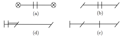
Figure 6: Brane setups for dual theories of $T[SU(2)]$. Horizontal/vertical/tilted lines represent D3/D5/(1,1)-branes. Crossed circles represent NS5-branes.

Appendix B Difference equations for $T[SU(2),\varphi]$ at classical limit

The index (109) of $T[SU(2)]$ can be constructed from tetrahedron indices ${\cal I}_{\Delta}$ as follows

$$I_{\varphi=S}(m_{b},m_{t},m_{\eta};u_{b},u_{t},u_{\eta})$$

$$=(-1)^{2m_{b}}{\cal I}_{\Delta}(-m_{\eta},u_{\eta}^{-1}q^{\frac{1}{2}})u_{\eta}^{m_{\eta}}\sum_{m_{s}}\oint\frac{du_{s}}{2\pi iu_{s}}u_{s}^{2m_{t}+2m_{s}}u_{t}^{2m_{s}}u_{b}^{2m_{b}}q^{-\frac{1}{4}m_{\eta}}$$

$$\quad\times\prod_{\epsilon_{1},\epsilon_{2}=\pm 1}{\cal I}_{\Delta}(\epsilon_{1}m_{b}+\frac{1}{2}m_{\eta}+\epsilon_{2}m_{s},u_{b}^{\epsilon_{1}}u_{\eta}^{\frac{1}{2}}u_{s}^{\epsilon_{2}}q^{\frac{1}{4}})\;.$$ (304)

In the charge basis, the index become

$$I_{\varphi=S}(m_{b},m_{t},m_{\eta};e_{b},e_{t},e_{\eta})=\sum_{e_{1},e_{2}\in\mathbb{Z}}\prod_{i=1}^{5}{\cal I}_{\Delta}(\tilde{m}_{i},\tilde{e}_{i})\;,\;\textrm{where}$$

$$(\tilde{m}_{1},\tilde{e}_{1})=(-m_{\eta}+\frac{\hbar}{2},e_{1}-\frac{\hbar}{4})\;,\;(\tilde{m}_{2},\tilde{e}_{2})=(m_{b}+\frac{1}{2}m_{\eta}+\frac{e_{t}}{2}+\frac{\hbar}{4},e_{2}-i\pi)\;,$$

$$(\tilde{m}_{3},\tilde{e}_{3})=(-m_{b}+\frac{1}{2}m_{\eta}-\frac{e_{t}}{2}+\frac{\hbar}{4},e_{2}-\frac{e_{b}}{2}+\frac{e_{t}}{2}+m_{b}+m_{t})\;,$$

$$(\tilde{m}_{4},\tilde{e}_{4})=(-m_{b}+\frac{1}{2}m_{\eta}+\frac{e_{t}}{2}+\frac{\hbar}{4},e_{1}-e_{2}+e_{\eta}-\frac{e_{t}}{2}-m_{\eta}-m_{t}+i\pi)\;,$$

$$(\tilde{m}_{5},\tilde{e}_{5})=(m_{b}+\frac{1}{2}m_{\eta}-\frac{e_{t}}{2}+\frac{\hbar}{4},e_{1}-e_{2}+\frac{e_{b}}{2}+e_{\eta}-m_{b}-m_{\eta})\;.$$ (305)

We have five difference equations for the index $\prod_{i=1}^{5}{\cal I}_{\Delta}(\tilde{m}_{i},\tilde{e}_{i})$,

$$\tilde{x}_{i}^{-1}+\tilde{p}_{i}-1=0\,,\qquad\mbox{for }i=1,2,\ldots,5\;.$$

where $\tilde{x}_{i},\tilde{p}_{i}$ can be written in terms of $(p_{1},p_{2},x_{b},x_{t},x_{\eta},p_{b},p_{t},p_{\eta})$ from eq. (305); see also (152)). We will focus on the classical limit, $\hbar\to 0$ from here on. In the classical limit,

$$\tilde{x}_{1}=\frac{1}{x_{\eta}},\quad\tilde{x}_{2}=p_{t}^{\frac{1}{2}}x_{b}x^{\frac{1}{2}}_{\eta},\quad\tilde{x}_{3}=p_{t}^{-\frac{1}{2}}x^{-1}_{b}x^{\frac{1}{2}}_{\eta},\quad\tilde{x}_{4}=p_{t}^{\frac{1}{2}}x^{-1}_{b}x^{\frac{1}{2}}_{\eta},\quad\tilde{x}_{5}=p_{t}^{-\frac{1}{2}}x_{b}x^{\frac{1}{2}}_{\eta}\,,$$

$$\tilde{p}_{1}=p_{1},\quad\tilde{p}_{2}=-p_{2},\quad\tilde{p}_{3}=\frac{p_{t}^{\frac{1}{2}}p_{2}x_{b}x_{t}}{p_{b}^{\frac{1}{2}}},\quad\tilde{p}_{4}=-\frac{p_{\eta}p_{1}}{p_{t}^{\frac{1}{2}}p_{2}x_{\eta}x_{t}},\quad\tilde{p}_{5}=\frac{p_{b}^{\frac{1}{2}}p_{\eta}p_{1}}{p_{2}x_{b}x_{\eta}}\,.$$

The summations $\sum_{e_{1},e_{2}}$ corresponds to integrating out $p_{1},p_{2}$ from difference equations. We use the first two equations, $\tilde{x}_{1}+\tilde{p}_{1}^{-1}-1=0$ and $\tilde{x}_{2}+\tilde{p}_{2}^{-1}-1=0$ to integrate out $p_{1},p_{2}$

$$p_{1}=1-x_{\eta},\quad p_{2}=\frac{1-p_{t}^{\frac{1}{2}}x_{b}x^{\frac{1}{2}}_{\eta}}{p_{t}^{\frac{1}{2}}x_{b}x_{\eta}^{\frac{1}{2}}}\,.$$ (306)

Thus we are left with three equations of six variables, $\tilde{x}_{i}^{-1}+\tilde{p}_{i}-1=0$ for $i=3,4,5$ where $p_{1},p_{2}$ in $\tilde{x}_{i},\tilde{p}_{i}$ are replaced by the above conditions

$$\{\tilde{x}_{i}^{-1}+\tilde{p}_{i}-1=0,\mbox{ for }i=3,4,5.\}/.\{p_{1}\to 1-x_{\eta},\ p_{2}\to\frac{1-p_{t}^{\frac{1}{2}}x_{b}x^{\frac{1}{2}}_{\eta}}{p_{t}^{\frac{1}{2}}x_{b}x^{\frac{1}{2}}_{\eta}}\}\,.$$ (307)

which are classical difference equations of $I_{\varphi=S}$. After some algebraic manipulations, the equations can be written as

$$x_{b}+x_{b}^{-1}=\frac{x^{\frac{1}{2}}_{\eta}x_{t}^{-1}-x_{\eta}^{-\frac{1}{2}}x_{t}}{x_{t}^{-1}-x_{t}}p_{t}^{-\frac{1}{2}}+\frac{x^{-\frac{1}{2}}_{\eta}x_{t}^{-1}-x^{\frac{1}{2}}_{\eta}x_{t}}{x_{t}^{-1}-x_{t}}p_{t}^{\frac{1}{2}}$$

$$\frac{x^{\frac{1}{2}}_{\eta}x_{b}-x_{\eta}^{-\frac{1}{2}}x_{b}^{-1}}{x_{b}-x_{b}^{-1}}p_{b}^{-\frac{1}{2}}+\frac{x^{-\frac{1}{2}}_{\eta}x_{b}-x^{\frac{1}{2}}_{\eta}x_{b}^{-1}}{x_{b}-x_{b}^{-1}}p_{b}^{\frac{1}{2}}=x_{t}+x_{t}^{-1}$$

$$p_{\eta}=\frac{p_{t}^{-\frac{1}{2}}-p_{t}^{\frac{1}{2}}}{x_{t}^{-1}-x_{t}}=\frac{x_{b}-x_{b}^{-1}}{p_{b}^{-\frac{1}{2}}-p_{b}^{\frac{1}{2}}}\;.$$ (308)

which are indeed the classical limit, $\hbar\to 0$ i.e. $q\to 1$, of the difference equations of $I_{\varphi=S}$ given in eq. (247). These equations are the same as algebraic equations studied in Gaiotto:2013bwa which define a moduli space of vacua for $T[SU(2)]$. In terms of shear operators (252), the classical difference equations are

$$\mathcal{L}_{\varphi=S}=\{(\sqrt{\mathsf{t}}^{\rm T})_{t}-(\frac{1}{\sqrt{\mathsf{t}}})_{b}=0\;,\;(\sqrt{\mathsf{t}^{\prime\prime}}^{\rm T})_{t}-\sqrt{\mathsf{t}^{\prime}}(1+\mathsf{t})_{b}=0\;,\;p_{\eta}=-\frac{i}{\sqrt{\mathsf{t}}_{b}}\}\;.$$ (309)

For $\varphi=T$, classical difference equations are (see eq. (257))

$$\mathcal{L}_{\varphi=T}=\{x_{t}=x_{b}\;,\;p_{t}^{-\frac{1}{2}}=p_{b}^{\frac{1}{2}}x_{b}^{-1}\;,\;p_{\eta}=1\}\;.$$ (310)

In terms of shear coordinates,

$$\mathcal{L}_{\varphi=T}=\{(\sqrt{\mathsf{t}}^{\rm T})_{t}-(\frac{1}{\sqrt{\mathsf{t}^{\prime}}})_{b}=0\;,\;(\sqrt{\mathsf{t}^{\prime\prime}}^{\rm T})_{t}-\sqrt{\mathsf{t}^{\prime\prime}}(1+\mathsf{t}^{\prime})_{b}=0\;,\;p_{\eta}=1\}\;.$$ (311)

A general $\varphi\in SL(2,\mathbb{Z})$ can be written as a product of $S$ and $T$. Thus, to obtain the classical difference equation for general $\varphi$, we only need to know the gluing rules for the classical difference equations. For $\varphi=\varphi_{2}\varphi_{1}$, the classical Lagrangian can be obtained by

1. Identify $(\sqrt{\mathsf{t}}^{\rm T},\sqrt{\mathsf{t}^{\prime}}^{\rm T},\sqrt{\mathsf{t}^{\prime\prime}}^{\rm T})_{t}$ of $\varphi_{2}$ with $(\sqrt{\mathsf{t}},\sqrt{\mathsf{t}^{\prime}},\sqrt{\mathsf{t}^{\prime\prime}})_{b}$ of $\varphi_{1}$.
2. If $p_{\eta}=p_{\eta,i}$ for $\varphi_{i=1,2}$, then $p_{\eta}=p_{\eta,2}p_{\eta,1}$ for $\varphi=\varphi_{2}\varphi_{1}$.
3. Integrate out $(\sqrt{\mathsf{t}}^{\rm T},\sqrt{\mathsf{t}^{\prime}}^{\rm T},\sqrt{\mathsf{t}^{\prime\prime}}^{\rm T})_{t}$ of $\varphi_{2}$ (or equivalently $(\sqrt{\mathsf{t}},\sqrt{\mathsf{t}^{\prime}},\sqrt{\mathsf{t}^{\prime\prime}})_{b}$ of $\varphi_{1}$) .

Using the gluing rules, the classical Lagrangian for $\varphi=S^{2}$ and $\varphi=(ST)^{3}$ become

$$\mathcal{L}_{\varphi=S^{2}}=\{(\sqrt{\mathsf{t}}^{\rm T})_{t}-(\sqrt{\mathsf{t}})_{b}=0\;,\;(\sqrt{\mathsf{t}^{\prime\prime}}^{\rm T})_{t}-(\sqrt{\mathsf{t}^{\prime\prime}})_{b}=0\;,\;p_{\eta}=-1\;\}$$

$$\mathcal{L}_{\varphi=(ST)^{3}}=\{(\sqrt{\mathsf{t}}^{\rm T})_{t}-(\sqrt{\mathsf{t}})_{b}=0\;,\;(\sqrt{\mathsf{t}^{\prime\prime}}^{\rm T})_{t}-(\sqrt{\mathsf{t}^{\prime\prime}})_{b}=0\;,\;p_{\eta}=\frac{-i}{\sqrt{\mathsf{t}_{b}\mathsf{t}^{\prime}_{b}\mathsf{t}^{\prime\prime}_{b}}}=x_{\eta}^{-\frac{1}{2}}\;\}\;.$$ (312)

In the last equation, we used the fact $\sqrt{\mathsf{t}\mathsf{t}^{\prime}\mathsf{t}^{\prime\prime}}=-ix^{\frac{1}{2}}_{\eta}$ in the classical limit. These classical difference equations reflect the $SL(2,\mathbb{Z})$ structure (120) for index $I_{\varphi}$.

Appendix C Derivation of eq. (230)

For $\varphi=\mathsf{L}$, let us first define a convenient basis $\{|(m,e)\rangle_{\Pi_{\mathsf{L}}}\}$ where the polarization $\Pi_{\mathsf{L}}$ is defined by

$$\Pi_{\mathsf{L}}=\big{(}{\cal X}_{\mathsf{L}},{\cal P}_{\mathsf{L}})_{\pm}=(-\mathsf{T}^{\prime\prime}_{\pm}\pm i\pi+\log\mathfrak{l}_{\pm}\mp\frac{\hbar}{2},\frac{1}{2}(\mathsf{T}_{\pm}+\mathsf{T}^{\prime\prime}_{\pm}-\log\mathfrak{l}_{\pm})\big{)}\;.$$ (313)

$\Pi_{\mathsf{L}}$ is related to the $\Pi_{\rm SR}$ in (182) in the following way

$$\left(\begin{array}[]{c}{\cal X}_{\mathsf{L}}\\ {\cal P}_{\mathsf{L}}\end{array}\right)_{\pm} =\left(\begin{array}[]{cc}2&0\\ -\frac{1}{2}&\frac{1}{2}\end{array}\right)\left(\begin{array}[]{c}{\cal X}_{\rm SR}\\ {\cal P}_{\rm SR}\end{array}\right)_{\pm}\pm\left(\begin{array}[]{c}-\frac{\hbar}{2}\\ \frac{i\pi}{2}\end{array}\right)\;\,.$$ (322)

In terms of ${\cal X}_{\mathsf{L}\pm},{\cal P}_{\mathsf{L}\pm}$ (position, momentum) operators in $\Pi_{\mathsf{L}}$, 솓 operator $\mathsf{L}$ in (95) can be written as

$$\mathsf{L}=\left(\prod_{r=1}^{\infty}\frac{1-q^{r}e^{{\cal X}_{\mathsf{L}+}}\mathfrak{l}^{-1}_{+}}{1-q^{r-1}e^{{\cal X}_{\mathsf{L}-}}\mathfrak{l}^{-1}_{-}}\right)\exp\big{[}-\frac{1}{\hbar}\big{(}({\cal P}_{\mathsf{L}+}+\frac{1}{2}\log\mathfrak{l}_{+})^{2}-({\cal P}_{\mathsf{L}-}+\frac{1}{2}\log\mathfrak{l}_{-})^{2}\big{)}\big{]}\;.$$ (323)

Let us suppress the subscript $\mathsf{L}$ of ${\cal X}_{\mathsf{L}\pm},{\cal P}_{\mathsf{L}\pm}$ hereafter. For instance, eq. (173) would be written as

$${}_{\mathsf{L}}\langle m,e|e^{{\cal X}_{\pm}}=\;_{\mathsf{L}}\langle m,e\mp 1|q^{\frac{m}{2}},\qquad_{\mathsf{L}}\langle m,e|e^{{\cal P}_{\pm}}=\;_{\mathsf{L}}\langle m\pm 1,e|q^{\frac{e}{2}}\,.$$ (324)

Using eq. (181), one can find a relation between ${}_{\mathsf{L}}\langle(m,e)|$ and ${}_{\rm SR}\langle(m,e)|$ such as

$${}_{\rm SR}\langle m,e| =_{\mathsf{L}}\langle 2m,\frac{1}{2}(e-m)|q^{\frac{1}{4}(m-e)}(-1)^{-m}\,,$$ (326)

$${}_{\mathsf{L}}\langle m,e| =_{\rm SR}\langle\frac{1}{2}m,2e+\frac{1}{2}m|q^{\frac{1}{2}e}(-1)^{\frac{m}{2}}\,.$$ (327)

The second equation results in the following inner product of ${}_{\mathsf{L}}\langle m,e|$ basis

$${}_{\mathsf{L}}\langle m_{2},e_{2}|m_{1},e_{1}\rangle_{\mathsf{L}}=q^{e_{1}}\delta_{m_{1},m_{2}}\delta_{e_{1},e_{2}}\;,$$ (328)

which follows from the inner product of SR basis given in eq. (184). Using eq. (326), The evaluation of $\mathsf{L}$ operator in ${}_{\rm SR}\langle m,e|$ basis can be rewritten as follows

$${}_{\rm SR}\langle(m_{2},e_{2}),(m_{\eta},e_{\eta})|\mathsf{L}|(m_{1},e_{1}),(m_{\eta},0)\rangle_{\rm SR}$$

$$=q^{\frac{1}{4}(m_{2}-e_{2}+m_{1}-e_{1})}(-1)^{-m_{2}+m_{1}}\;_{\mathsf{L}}\langle(2m_{2},\frac{e_{2}-m_{2}}{2}),(m_{\eta},e_{\eta})|\mathsf{L}|(2m_{1},\frac{e_{1}-m_{1}}{2}),(m_{\eta},0)\rangle_{\mathsf{L}}$$ (329)

To evaluate the right hand side, we first note that the infinite product part of $\mathsf{L}$ operator acts on the bra as follows

$${}_{\mathsf{L}}\langle(m_{2},e_{2}),(m_{\eta},e_{\eta})|\prod_{r=1}^{\infty}\frac{1-q^{r}e^{{\cal X}_{+}}\mathfrak{l}^{-1}_{+}}{1-q^{r-1}e^{{\cal X}_{-}}\mathfrak{l}^{-1}_{-}}$$

$$=\oint\frac{du_{2}}{2\pi iu_{2}}\oint\frac{du_{\eta}}{2\pi iu_{\eta}}u^{-e_{2}}u_{\eta}^{-e_{\eta}}\;{}_{\mathsf{L}}\langle(m_{2},u_{2}),(m_{\eta},u_{\eta})|\prod_{r=1}^{\infty}\frac{1-q^{r}e^{{\cal X}_{+}}\mathfrak{l}^{-1}_{+}}{1-q^{r-1}e^{{\cal X}_{-}}\mathfrak{l}^{-1}_{-}}$$

$$=\sum_{e^{\prime}}\;{}_{\mathsf{L}}\langle(m_{2},e_{2}+e^{\prime}),(m_{\eta},e_{\eta}-e^{\prime})|{\cal I}_{\Delta}(m_{\eta}-m_{2},e^{\prime})\;,$$ (330)

and that the exponential part of $\mathsf{L}$ operator acts on the ket as follows

$$\exp\big{[}-\frac{1}{\hbar}(({\cal P}_{+}+\frac{1}{2}\log\mathfrak{l}_{+})^{2}-({\cal P}_{-}+\frac{1}{2}\log\mathfrak{l}_{-})^{2})\big{]}|(m_{1},e_{1}),(m_{\eta},e_{\eta})\rangle_{\mathsf{L}}$$

$$=(\;_{\mathsf{L}}\langle(m_{1},e_{1}),(m_{\eta},e_{\eta})|\exp\big{[}-\frac{1}{\hbar}(({\cal P}_{-}+\frac{1}{2}\log\mathfrak{l}_{-})^{2}-({\cal P}_{+}+\frac{1}{2}\log\mathfrak{l}_{+})^{2})\big{]})^{\dagger}$$

$$=|(m_{1}+2e_{1}+m_{\eta},e_{1}),(m_{\eta},e_{\eta}-e_{1}-\frac{1}{2}m_{\eta})\rangle_{\mathsf{L}}\,.$$ (331)

Here we used the fact that the adjoint of operators are given by

$$({\cal P}_{\pm,\mathsf{L}})^{\dagger}={\cal P}_{\mp,\mathsf{L}},\quad(\mathfrak{l}_{\pm})^{\dagger}=\mathfrak{l}_{\mp}\;,$$ (332)

and that they can be written as ${\cal P}_{\pm}=\pm\partial_{m}+\frac{\hbar}{2}e,\ln\mathfrak{l}_{\pm}=\mp\partial_{e_{\eta}}+\frac{\hbar}{2}m_{\eta}$. Using eq. (330), (331), and then (328), the evaluation of $\mathsf{L}$ operator in eq. (329) can be rewritten as

$${}_{\rm SR}\langle(m_{2},e_{2}),(m_{\eta},e_{\eta})|\mathsf{L}|(m_{1},e_{1}),(m_{\eta},0)\rangle_{\rm SR}$$

$$=\delta_{\ldots}\delta_{\ldots}(-1)^{m_{1}-m_{2}}q^{\frac{1}{4}(e_{1}-e_{2}-m_{1}+m_{2})}{\cal I}_{\Delta}(m_{\eta}-2m_{2},\frac{1}{2}(e_{1}-e_{2}-m_{1}+m_{2}))\;$$

$$=\delta_{\ldots}\delta_{\ldots}(-1)^{e_{2}-e_{1}}q^{\frac{1}{4}(e_{1}-e_{2}-m_{1}+m_{2})}{\cal I}_{\Delta}(-e_{1}-m_{1},\frac{1}{2}(e_{1}-e_{2}-m_{1}+m_{2}))$$

$$=\delta_{\ldots}\delta_{\ldots}(-1)^{e_{2}-e_{1}}q^{\frac{1}{4}(e_{1}-e_{2}-m_{1}+m_{2})}{\cal I}_{\Delta}(\frac{-e_{1}+m_{1}+e_{2}-m_{2}}{2},m_{1}+e_{1})$$

where $\delta_{\ldots}\delta_{\ldots}$ denotes the following combination of Kronecker delta functions,

$$\delta_{\ldots}\delta_{\ldots} =\delta(-e_{1}+2m_{2}-m_{1}-m_{\eta})\delta(e_{2}-e_{1}+2e_{\eta}+m_{2}-m_{1})\;.$$ (333)

In the third line, we changed the first argument in the tetrahedron index and the power of $(-1)$ using Kronecker delta functions. In the last line, we used the identity of ${\cal I}_{\Delta}$ in eq. (154). This completes the derivation of the first part of (230).

For $\varphi=\mathsf{R}$, we basically repeat the previous derivation for $\varphi=\mathsf{L}$ using a polarization $\Pi_{\mathsf{R}}$ instead of the polarization $\Pi_{\mathsf{L}}$. $\Pi_{\mathsf{R}}$ is defined by

$$\Pi_{\mathsf{R}}=({\mathcal{X}}_{\mathsf{R}},{\mathcal{P}}_{\mathsf{R}})_{\pm}=(\mathsf{T}^{\prime}_{\pm}\pm i\pi\pm\frac{\hbar}{2},\frac{1}{2}(\mathsf{T}^{\prime}_{\pm}+\mathsf{T}_{\pm}))\;,$$ (334)

thus it is related to $\Pi_{\rm SR}$ as follows

$$\begin{pmatrix}{\mathcal{X}_{\mathsf{R}}}\\ {\mathcal{P}_{\mathsf{R}}}\end{pmatrix}_{\pm}=\begin{pmatrix}1&-1\\ 1&0\end{pmatrix}\cdot\begin{pmatrix}{\mathcal{X}}_{\rm SR}\\ {\mathcal{P}}_{\rm SR}\end{pmatrix}_{\pm}\pm\begin{pmatrix}\frac{\hbar}{2}+i\pi\\ 0\end{pmatrix}$$ (335)

In terms of momentum and position operators in this polarization, $\mathsf{R}$ operator in (95) can be written as

$$\mathsf{R}=\left(\prod_{r=1}^{\infty}\frac{1-q^{r}e^{{\mathcal{X}}_{\mathsf{R}-}}}{1-q^{r-1}e^{{\mathcal{X}}_{\mathsf{R}+}}}\right)\exp[\frac{1}{\hbar}({\mathcal{P}}_{\mathsf{R}+}^{2}-{\mathcal{P}}_{\mathsf{R}-}^{2})]\;.$$ (336)

The basis change between SR- and $\mathsf{R}$-basis can be obtained as

$${}_{\rm SR}\langle m,e|=_{\mathsf{R}}\langle m-e,m|(-1)^{m}q^{\frac{m}{2}}\;,\quad_{\mathsf{R}}\langle m,e|=_{\rm SR}\langle e,e-m|(-1)^{-e}q^{-\frac{e}{2}}\;,$$

where the inner product of $\mathsf{R}$-basis is

$${}_{\mathsf{R}}\langle m_{2},e_{2}|m_{1},e_{1}\rangle_{\mathsf{R}}=\delta_{m_{1},m_{2}}\delta_{e_{1},e_{2}}q^{-e_{2}}\;.$$

In the ${}_{\mathsf{R}}\langle m,e|$ basis, the expectation value of $\mathsf{R}$ can be evaluated similarly to eq. (330) and (331), which results in

$${}_{\mathsf{R}}\langle(m_{2},e_{2})|\mathsf{R}|(m_{1},e_{1})\rangle_{\mathsf{R}}=\sum_{e^{\prime}}{\cal I}_{\Delta}(-m_{2},e^{\prime})_{\mathsf{R}}\langle m_{2},e_{2}-e^{\prime}|m_{1}-2e_{1},e_{1}\rangle_{\mathsf{R}}\;.$$

To evaluate the charge shifts of the ket basis, we used the adjoint relation of ${\mathcal{P}_{\mathsf{R},\pm}}$

$$({\mathcal{P}_{\mathsf{R},\pm}})^{\dagger}={\mathcal{P}_{\mathsf{R},\mp}}\,$$ (337)

which can be deduced from the adjoint relation of ${\mathcal{P}}_{\rm SR,\pm}$. Thus, we obtain

$${}_{\rm SR}\langle m_{2},e_{2}|\mathsf{R}|m_{1},e_{1}\rangle_{\rm SR} =(-1)^{m_{2}-m_{1}}q^{\frac{m_{1}+m_{2}}{2}}_{\mathsf{R}}\langle m_{2}-e_{2},m_{2}|\mathsf{R}|m_{1}-e_{1},m_{1}\rangle_{\mathsf{R}}$$

$$=(-1)^{m_{2}+e_{1}}q^{\frac{1}{2}(m_{2}+e_{1})}{\cal I}_{\Delta}(-e_{1}-m_{2},m_{1}+e_{1})\delta_{m_{2}+m_{1}-e_{2}+e_{1},0}\,.$$

In the second line, the Kronecker delta function was used to change the first argument of ${\cal I}_{\Delta}$, then the triality relation (153) was used in turn. This gives a derivation for the second part in eq. (230).

Appendix D Basis change between SR and FN basis

Recall that $\Pi_{\rm SR}=({\cal S},{\cal R}):=(\frac{1}{2}(\mathsf{T}+\mathsf{T}^{\prime}),\frac{1}{2}(\mathsf{T}-\mathsf{T}^{\prime}))$. Explicit expressions for $\mathsf{s}=\exp(\mathcal{S}),\mathsf{r}=\exp(\mathcal{R})$ in terms of Fenchel-Nielsen operators, $(\hat{\lambda},\hat{\tau})$ are given by

$$\mathsf{s}_{\pm}=\exp({\cal S}_{\pm})=q^{\pm 1/4}\frac{1}{(q^{\mp 1/4}\hat{\lambda}^{-1}_{\pm}\hat{\tau}_{\pm}^{1/2}-q^{\pm 1/4}\hat{\tau}_{\pm}^{-1/2}\hat{\lambda}_{\pm})}(\hat{\tau}_{\pm}^{1/2}-\hat{\tau}_{\pm}^{-1/2})\;.$$

$$\mathsf{r}_{\pm}=\exp({\cal R}_{\pm})=q^{\pm 1/4}\frac{1}{\hat{\lambda}_{\pm}-\hat{\lambda}_{\pm}^{-1}}(\hat{\tau}^{-1/2}_{\pm}-\hat{\tau}^{1/2}_{\pm})\frac{1}{\hat{\lambda}_{\pm}-\hat{\lambda}_{\pm}^{-1}}(q^{\mp 1/4}\hat{\lambda}^{-1}_{\pm}\hat{\tau}_{\pm}^{1/2}-q^{\pm 1/4}\hat{\tau}_{\pm}^{-1/2}\hat{\lambda}_{\pm})\;.$$ (338)

We will express SR fugacity basis $\langle m,u|:=_{\widetilde{\rm SR}}\langle m,u|$ in terms of FN fugacity basis $\langle\tilde{m},\tilde{u}|:=_{\rm FN}\langle\tilde{m},\tilde{u}|$,

$$\langle m,u|=\oint\frac{d\tilde{u}}{2\pi i\tilde{u}}\Delta(\tilde{m},\tilde{u},q)\langle m,u|\tilde{m},\tilde{u}\rangle\langle\tilde{m},\tilde{u}|\;.$$ (339)

By imposing the following conditions, we obtain difference equations for the basis change coefficients $\langle m,u|\tilde{m},\tilde{u}\rangle$.

$$\langle m,u|\mathsf{s}_{\pm}|\tilde{m},\tilde{u}\rangle =x_{\pm}\cdot\langle m,u|\tilde{m},\tilde{u}\rangle$$

$$=\langle m,u|\mathsf{s}_{\pm}(\hat{\lambda}_{\pm},\hat{\tau}_{\pm})|\tilde{m},\tilde{u}\rangle=s_{\pm}^{T}(\tilde{x}_{\pm},\tilde{p}_{\pm})\cdot\langle m,u|\tilde{m},\tilde{u}\rangle$$

$$\langle m,u|\mathsf{r}_{\pm}|\tilde{m},\tilde{u}\rangle =p_{\pm}\cdot\langle m,u|\tilde{m},\tilde{u}\rangle$$

$$=\langle m,u|\mathsf{r}_{\pm}(\hat{\lambda}_{\pm},\hat{\tau}_{\pm})|\tilde{m},\tilde{u}\rangle=r_{\pm}^{T}(\tilde{x}_{\pm},\tilde{p}_{\pm})\cdot\langle m,u|\tilde{m},\tilde{u}\rangle\;.$$ (340)

Here $\mathsf{O}^{\rm T}$ denote the transpose of $\mathsf{O}$, $\mathsf{O}_{\pm}^{\rm T}:=(\mathsf{O}^{\dagger}_{\pm})^{*}$. For SR operators, their transpose operators are

$$(\mathsf{s}_{\pm},\mathsf{r}_{\pm})^{\rm T}=(\mathsf{s}_{\pm},\mathsf{r}_{\pm})/.\{q\rightarrow q^{-1},\tau\rightarrow\tau^{-1}\}\;.$$ (341)

The operators $(x,p)_{\pm},(\tilde{x},\tilde{p})_{\pm}$ are given

$$x_{\pm}=q^{\frac{m}{2}}u^{\pm 1}\;,\quad p_{\pm}=e^{\pm\partial_{m}+\frac{1}{2}\hbar u\partial_{u}}\;,\quad\tilde{x}_{\pm}=q^{\frac{\tilde{m}}{2}}\tilde{u}^{\pm 1}\;,\quad\tilde{p}_{\pm}=e^{\pm\partial_{\tilde{m}}+\frac{1}{2}\hbar\tilde{u}\partial_{\tilde{u}}}\;.$$ (342)

To make the action of FN, SR operators simple, we introduce new variables $(a,b),(s,t)$ defined as follow

$$q^{a}:=q^{\frac{\tilde{m}}{2}}\tilde{u},\quad q^{b}=q^{\frac{\tilde{m}}{2}}\tilde{u}^{-1},\quad q^{s}:=q^{\frac{m}{2}}u,\quad q^{t}=q^{\frac{m}{2}}u^{-1}\;.$$ (343)

Let’s denote $\langle m,u|\tilde{m},\tilde{u}\rangle$ in terms of these variables as $C(a,b|s,t)$.

$$C(a,b|s,t):=\langle m,u|\tilde{m},\tilde{u}\rangle/.\{\tilde{m}\rightarrow a+b,m\rightarrow s+t,\tilde{u}\rightarrow q^{\frac{a-b}{2}},u\rightarrow q^{\frac{s-t}{2}}\}\;.$$ (344)

One advantage of these variables is that $+$ ($-$) type operators act only on $a,s$ ($b,t$) variables. Thus the difference equations (340) for $C(s,t|a,b)$ factorizes into $\pm$ parts and we can set

$$C(s,t|a,b)=C_{+}(s|a)C_{-}(t|b)\;.$$ (345)

Then, the difference equations for $C_{+}$ are

$$(1-q^{-a+s})C_{+}(s|a)=(1-q^{s+a+1})C_{+}(s|a+1)\;,$$

$$(q^{a}-q^{-a})C_{+}(s+1|a)$$

$$=\frac{q^{-(a+1/2)}C_{+}(s|a)-q^{a+1/2}C_{+}(s|a+1)}{q^{a+1/2}-q^{-(a+1/2)}}-\frac{q^{-(a-1/2)}C_{+}(s|a-1)-q^{a-1/2}C_{+}(s|a)}{q^{a-1/2}-q^{-(a-1/2)}}\;.$$

For $C_{-}$, the difference equations are

$$(1-q^{b+t})C_{-}(t|b)=(1-q^{t-b-1})C_{-}(t|b+1)\;,$$

$$(q^{b}-q^{-b})C_{-}(t-1|b)$$

$$=\frac{q^{-(b-1/2)}C_{-}(t|b)-q^{b-1/2}C_{-}(t|b-1)}{q^{b-1/2}-q^{-(b-1/2)}}-\frac{q^{-(b+1/2)}C_{-}(t|b+1)-q^{b+1/2}C_{-}(t|b)}{q^{b+1/2}-q^{-(b+1/2)}}\;.$$ (346)

We use the fact that

$$(x_{+},x_{-},p_{+},p_{-})=(q^{s},q^{t},e^{\partial_{s}},e^{-\partial_{t}})\;,\quad(\tilde{x}_{+},\tilde{x}_{-},\tilde{p}_{+},\tilde{p}_{-})=(q^{a},q^{b},e^{\partial_{a}},e^{-\partial_{b}})\;.$$ (347)

Solving the two difference equations, we find the following solutions

$$C_{+}(s|a)=(-1)^{a}q^{-a(a+1)/2-as}\prod_{r=0}^{\infty}\frac{1-q^{r+1}q^{-a+s}}{1-q^{r}q^{-a-s}}\;,$$

$$C_{-}(t|b)=(-1)^{b}q^{b(b-1)/2+bt}\prod_{r=0}^{\infty}\frac{1-q^{r+1}q^{-b-t}}{1-q^{r}q^{-b+t}}\;.$$

Therefore,

$$C(s,t|a,b)=(-1)^{a+b}q^{-a(a+1)/2-as+b(b-1)/2+bt}\prod_{r=0}^{\infty}\frac{1-q^{r+1}q^{-a+s}}{1-q^{r}q^{-a-s}}\prod_{r=0}^{\infty}\frac{1-q^{r+1}q^{-b-t}}{1-q^{r}q^{-b+t}}\;.$$ (348)

In the original fugacity variables$(m,u),(\tilde{m},\tilde{u})$, the basis change matrix is given by

$$\langle m,u|\tilde{m},\tilde{u}\rangle=C(s,t|a,b)|_{a\rightarrow\frac{\tilde{m}}{2}+\log_{q}\tilde{u},b\rightarrow\frac{\tilde{m}}{2}-\log_{q}\tilde{u},s\rightarrow\frac{m}{2}+\log_{q}u,t\rightarrow\frac{m}{2}+\log_{q}u}$$

$$=(-\tilde{u}q^{1/2})^{-\tilde{m}}\frac{{\cal I}_{\Delta}(\tilde{m}-m,\tilde{u}/u)}{{\cal I}_{\Delta}(\tilde{m}+m,u\tilde{u}q^{-1})}u^{-\tilde{m}}\tilde{u}^{-m}\;,$$

$$=(-q^{\frac{1}{2}}u)^{m}{\cal I}_{\Delta}(-m-\tilde{m},u^{-1}\tilde{u}^{-1}){\cal I}_{\Delta}(\tilde{m}-m,\tilde{u}/u)\;.$$ (349)

In the SR charge basis, we have

$$\langle m,e|\tilde{m},\tilde{u}\rangle=\sum_{e_{1}\in\mathbb{Z}}(-q^{\frac{1}{2}})^{m}\tilde{u}^{-2e_{1}-e+m}{\cal I}_{\Delta}(-m-\tilde{m},e_{1}){\cal I}_{\Delta}(-m+\tilde{m},-e+m-e_{1})\;.$$ (350)

This basis change matrix element can be thought of as $SL(2,\mathbb{C})$ CS partition function on a mapping cylinder $\Sigma_{1,1}\times_{\varphi}I$ with $\varphi=\textrm{identity}$ in the polarization where positions are $(\mathsf{s}_{\textrm{bot}},\lambda_{\rm top},\mathfrak{l})$ and momenta are $(\mathsf{r}_{\rm bot},\tau_{\rm top},\mathfrak{m})$. Identifying FN operators $(\lambda,\tau)$ as UV operators and SR operator $(\mathsf{s},\mathsf{r})$ as IR operators, the mapping cylinder is called a RG manifold in Dimofte:2013lba .

Note that the SR basis is Weyl-reflection invariant and thus the states are in $\mathcal{H}_{SL(2,\mathbb{C})}\subset\widetilde{{\cal H}}_{SL(2,\mathbb{C})}$. For the charge basis $|m,e\rangle$ to be an (non-zero) element in $\mathcal{H}_{SL(2,\mathbb{C})}$, we need to impose following conditions

$$\langle m,e|\tilde{m},\tilde{u}\rangle\neq 0\;,\quad\textrm{for some $\tilde{m}\in\mathbb{Z}/2$}\;.$$ (351)

This condition implies that

$$m,e\in\mathbb{Z}/2,\quad m+e\in\mathbb{Z}\;.$$ (352)

Furthermore, we claim that SR charge basis are complete basis for $\mathcal{H}_{SL(2,\mathbb{C})}$. How can we prove the completeness? One simple answer uses the fact that a operator $\mathsf{s}_{+}\mathsf{s}_{-}$ is self-adjoint. Since $\langle m,e|$ are eigenstates for the operator with eigenvalues $q^{m}$, they form a complete basis. Using the property $(\mathsf{s}_{\pm},\mathsf{r}_{\pm})^{\dagger}=(\mathsf{s}_{\mp},\mathsf{r}_{\mp})$ and

$$\langle m,e|\mathsf{s}_{+}=\langle m,e\mp 1|q^{\frac{m}{2}}\;,\quad\langle m,e|\mathsf{r}_{\pm}=\langle m\pm 1,e|q^{\frac{e}{2}}\;,$$ (353)

One can see that

$$\langle m,e|m^{\prime},e^{\prime}\rangle=\kappa\delta_{m,m^{\prime}}\delta_{e,e^{\prime}}\;.$$ (354)

Here $\kappa$ is $(m,e)$-independent constant and it is 1 in (349). From this orthonormality and the fact the basis $\langle m,e|$ are complete basis in $\mathcal{H}_{SL(2,\mathbb{C})}$, one obtain following completeness relation

$$\mathds{1}_{\mathcal{H}_{SL(2,\mathbb{C})}}=\sum_{(m,e)}|m,e\rangle\langle m,e|\;.$$ (355)

More directly, the completeness relation is equivalent to the following identity,

$$\sum_{(m,e)}\langle\tilde{m}_{b},\tilde{u}_{b}|m,e\rangle\langle m,e|\tilde{m}_{t},\tilde{m}_{t}\rangle=\delta(\tilde{m}_{b}-\tilde{m}_{t})\frac{\delta(\tilde{u}_{b}-\tilde{u}_{t})}{\Delta(\tilde{m}_{t},\tilde{u}_{t})}\;.$$

using the explicit expression in (350). While we do not have an exact proof, we have confirmed it by series expansion in $q$. More precisely, we checked that

$$\sum_{\tilde{m}\in\mathbb{Z}/2}\oint\frac{d\tilde{u}_{t}}{2\pi i\tilde{u}_{t}}\Delta(\tilde{m}_{t},\tilde{m}_{t})\big{(}\sum_{(m,e)}\langle\tilde{m}_{b},\tilde{u}_{b}|m,e\rangle\langle m,e|\tilde{m}_{t},\tilde{m}_{t}\rangle\big{)}f(\tilde{m}_{t},\tilde{u}_{t})=f(\tilde{m}_{b},\tilde{u}_{b})\;,$$

by expansion in $q$ for various Weyl-reflection invariant trial function $f(m,u)$, i.e., $f(m,u)=f(-m,u^{-1})$.

References

• (1) L. Alday, D. Gaiotto, Y. Tachikawa “Liouville Correlation Functions from Four-dimensional Gauge Theories,” Lett.Math.Phys.91 (2010) 167. arXiv:0906.3219 [hep-th]
• (2) D. Gaiotto “N=2 dualities,” arXiv:0904.2715 [hep-th].
• (3) V. Pestun “Localization of gauge theory on a four-sphere and supersymmetric Wilson loops,” Commun.Math.Phys. 313 (2012) 71-129 arXiv:0712.2824 [hep-th].
• (4) See, for example, the following review and references therein. Yu Nakayama “Liouville Field Theory – A decade after the revolution, ” Int.J.Mod.Phys.A19: (2004) 2771, arXiv:hep-th/0402009 [hep-th].
• (5) C. Cordova and D. L. Jafferis, arXiv:1305.2891 [hep-th].
• (6) T. Dimofte, D. Gaiotto and S. Gukov, “Gauge Theories Labelled by Three-Manifolds,” arXiv:1108.4389 [hep-th].
• (7) T. Dimofte, D. Gaiotto, and S. Gukov, “3-Manifolds and 3d Indices,” arXiv:1112.5179 [hep-th].
• (8) N. Hama, K. Hosomichi and S. Lee, “SUSY Gauge Theories on Squashed Three-Spheres,” JHEP 1105, 014 (2011) [arXiv:1102.4716 [hep-th]].
• (9) Y. Terashima and M. Yamazaki, “$SL(2,R)$ Chern-Simons, Liouville, and Gauge Theory on Duality Walls,” JHEP 1108 (2011) 135 [arXiv:1103.5748 [hep-th]].
• (10) J. Yagi, “3d TQFT from 6d SCFT,” arXiv:1305.0291 [hep-th].
• (11) D. Gaiotto and E. Witten, “S-Duality of Boundary Conditions In N=4 Super Yang-Mills Theory,” Adv. Theor. Math. Phys.  13 (2009) [arXiv:0807.3720 [hep-th]].
• (12) N. Drukker, D. Gaiotto and J. Gomis, “The Virtue of Defects in 4D Gauge Theories and 2D CFTs,” JHEP 1106, 025 (2011) [arXiv:1003.1112 [hep-th]].
• (13) K. Hosomichi, S. Lee and J. Park, “AGT on the S-duality Wall,” JHEP 1012, 079 (2010) [arXiv:1009.0340 [hep-th]].
• (14) Y. Terashima and M. Yamazaki, “Semiclassical Analysis of the 3D/3D Relation,” arXiv:1106.3066 [hep-th].
• (15) T. Dimofte and S. Gukov, “Chern-Simons Theory and S-duality,” arXiv:1106.4550 [hep-th].
• (16) J. Teschner and G. S. Vartanov, “6j symbols for the modular double, quantum hyperbolic geometry, and supersymmetric gauge theories,” arXiv:1202.4698 [math-ph].
• (17) D. Gang, E. Koh and K. Lee, “Superconformal Index with Duality Domain Wall,” arXiv:1205.0069 [hep-th].
• (18) K. Nagao, Y. Terashima, and M. Yamazaki, “Hyperbolic geometry and cluster algebra,” preprint (2011), arXiv:1112.3106 [math.GT].
• (19) Rinat M. Kashaev, Feng Luo, and Grigory Vartanov, “A TQFT of turaev-viro type on shaped triangulations,” preprint (2012), arXiv:1210.8393 [math.QA].
• (20) K. Hikami and R. Inoue, “Cluster algebra and complex volume of once-punctured torus bundles and two-bridge knots,” preprint (2012), arXiv:1212.6042 [math.GT].
• (21) Y. Terashima and M. Yamazaki, “3d N=2 Theories from Cluster Algebras,” arXiv:1301.5902 [hep-th].
• (22) K. Hikami and R. Inoue, “Braids, Complex Volume, and Cluster Algebra,” arXiv:1304.4776 [math.GT]
• (23) T. Dimofte, “Quantum Riemann Surfaces in Chern-Simons Theory,” arXiv:1102.4847 [hep-th].
• (24) F. Guéritaud and D. Futer, “On canonical triangulations of once-punctured torus bundles and two-bridge link complements,” Geom. Topol. 10, 1239 (2006).
• (25) T. Dimofte, M. Gabella and A. B. Goncharov, “K-Decompositions and 3d Gauge Theories,” arXiv:1301.0192 [hep-th].
• (26) Stavros Garoufalidis, Craig D. Hodgson, Hyam Rubinstein, and Henry Segerman, “1-efficient triangulations and the index of a cusped hyperbolic 3-manifold,” arXiv:1303.5278 [math.GT].
• (27) E. Witten, “SL(2,Z) action on three-dimensional conformal field theories with Abelian symmetry,” In *Shifman, M. (ed.) et al.: From fields to strings, vol. 2* 1173-1200 [hep-th/0307041].
• (28) S. Elitzur, G. W. Moore, A. Schwimmer and N. Seiberg, “Remarks on the canonical quantization of the Chern-Simons-Witten theory,” Nucl. Phys. B 326 (1989) 108.
• (29) Atiyah, Michael. “Topological quantum field theories.” Publications Mathmatiques de l’IHS 68.1 (1988): 175-186.
• (30) E. Witten, “Quantization of Chern-Simons Gauge Theory with Complex Gauge Group,” Commun. Math. Phys 137 (1991) 29–66.
• (31) V. V. Fock, “Description of moduli space of projective structures via fat graphs,” hep-th/9312193.
• (32) V. V. Fock, “Dual Teichmuller space,” dg-ga/9702018v3.
• (33) S. Gukov, “Three-dimensional quantum gravity, Chern-Simons theory, and the A polynomial,” Commun. Math. Phys.  255, 577 (2005) [hep-th/0306165].
• (34) S. Kim, “The Complete superconformal index for N=6 Chern-Simons theory,” Nucl. Phys. B 821, 241 (2009) [arXiv:0903.4172 [hep-th]].
• (35) Y. Imamura and S. Yokoyama, “Index for three dimensional superconformal field theories with general R-charge assignments,” JHEP 1104, 007 (2011) [arXiv:1101.0557 [hep-th]].
• (36) C. Krattenthaler, V. P. Spiridonov and G. S. Vartanov, “Superconformal indices of three-dimensional theories related by mirror symmetry,” JHEP 1106, 008 (2011) [arXiv:1103.4075 [hep-th]].
• (37) A. Kapustin and B. Willett, “Generalized Superconformal Index for Three Dimensional Field Theories,” arXiv:1106.2484 [hep-th].
• (38) D. Tong, “Dynamics of N=2 supersymmetric Chern-Simons theories,” JHEP 0007, 019 (2000) [hep-th/0005186].
• (39) Y. Imamura and D. Yokoyama, “$S^{3}/Z_{n}$ partition function and dualities,” JHEP 1211, 122 (2012) [arXiv:1208.1404 [hep-th]].
• (40) O. J. Ganor, Y. P. Hong and H. S. Tan, “Ground States of S-duality Twisted N=4 Super Yang-Mills Theory,” JHEP 1103, 099 (2011) [arXiv:1007.3749 [hep-th]].
• (41) O. J. Ganor, Y. P. Hong, R. Markov and H. S. Tan, “Static Charges in the Low-Energy Theory of the S-Duality Twist,” JHEP 1204, 041 (2012) [arXiv:1201.2679 [hep-th]].
• (42) Stavros Garoufalidis, “The 3D index of an ideal triangulation and angle structures,” arXiv:1208.1663 [math.GT].
• (43) E. Witten, “Analytic Continuation Of Chern-Simons Theory,” arXiv:1001.2933 [hep-th].
• (44) N. Nekrasov and E. Witten, “The Omega Deformation, Branes, Integrability, and Liouville Theory,” JHEP 1009, 092 (2010) [arXiv:1002.0888 [hep-th]].
• (45) G. Vartanov and J. Teschner, “Supersymmetric gauge theories, quantization of moduli spaces of flat connections, and conformal field theory,” arXiv:1302.3778 [hep-th].
• (46) L. Chekhov and V. V. Fock, “Quantum Teichmuller Space,” Theor. Math. Phys. 120 (1999) 1245 [Teor. Mat. Fiz. 120 (1999) 511] [math/9908165 [math-qa]].
• (47) R. M. Kashaev, “Quantization of Teichmüller spaces and the quantum dilogarithm,” Lett. Math.Phys. 43 (1998), no. 2 105–115.
• (48) J. Teschner, “An Analog of a Modular Functor from Quantized Teichmüller Theory,” in Handbook of Teichmuller Theory, Vol. I (2007) 685–760, [math/0510174v4].
• (49) J. Teschner, “On the relation between quantum Liouville theory and the quantized Teichmuller spaces,” Int. J. Mod. Phys. A 19S2, 459 (2004) [hep-th/0303149].
• (50) H. Verlinde, “Conformal field theory, two-dimensional quantum gravity and quantization of Teichmüller space,” Nucl. Phys. B 337 (1990) 652.
• (51) A. Gadde, E. Pomoni, L. Rastelli and S. S. Razamat, “S-duality and 2d Topological QFT,” JHEP 1003, 032 (2010) [arXiv:0910.2225 [hep-th]].
• (52) A. Gadde, L. Rastelli, S. S. Razamat and W. Yan, “The 4d Superconformal Index from q-deformed 2d Yang-Mills,” Phys. Rev. Lett.  106, 241602 (2011) [arXiv:1104.3850 [hep-th]].
• (53) D. Gang, E. Koh, K. Lee and , “Line Operator Index on $S^{1}\times S^{3}$,” JHEP 1205, 007 (2012) [arXiv:1201.5539 [hep-th]].
• (54) M. Aganagic, A. Klemm, M. Marino, C. Vafa and , “Matrix model as a mirror of Chern-Simons theory,” JHEP 0402, 010 (2004) [hep-th/0211098].
• (55) D. Gaiotto, L. Rastelli and S. S. Razamat, “Bootstrapping the superconformal index with surface defects,” arXiv:1207.3577 [hep-th].
• (56) L. F. Alday, M. Bullimore, M. Fluder and L. Hollands, “Surface defects, the superconformal index and q-deformed Yang-Mills,” arXiv:1303.4460 [hep-th].
• (57) C. Beem, T. Dimofte and S. Pasquetti, “Holomorphic Blocks in Three Dimensions,” arXiv:1211.1986 [hep-th].
• (58) C. Hwang, H. -C. Kim and J. Park, “Factorization of the 3d superconformal index,” arXiv:1211.6023 [hep-th].
• (59) R.M. Kashaev, In: S. Pakuliak and G. von Gehlen (eds.), Integrable structures of exactly solvable two-dimensional models of quantum field theory (Kiev, 2000), 211221, NATO Sci. Ser. II Math. Phys. Chem., 35, Kluwer Acad. Publ., Dordrecht, 2001.
• (60) L. D. Faddeev, “Discrete Heisenberg-Weyl Group and Modular Group,” Lett. Math. Phys. 34 (1995) 249 [hep-th/9504111].
• (61) D. Gaiotto and P. Koroteev, “On Three Dimensional Quiver Gauge Theories and Integrability,” arXiv:1304.0779 [hep-th].
• (62) T. Dimofte, D. Gaiotto and R. van der Veen, “RG Domain Walls and Hybrid Triangulations,” arXiv:1304.6721 [hep-th].