Redshift-space distortions from the cross-correlation of photometric populations

Abstract

Several papers have recently highlighted the possibility of measuring redshift space distortions from angular auto-correlations of galaxies in photometric redshift bins. In this work we extend this idea to include as observables the cross-correlations between redshift bins, as an additional way of measuring radial information. We show that this extra information allows to reduce the recovered error in the growth rate index $\gamma$ by a factor of $\sim 2$. Although the final error in $\gamma$ depends on the bias and the mean photometric accuracy of the galaxy sample, the improvement from adding cross-correlations is robust in different settings. Another factor of $2-3$ improvement in the determination of $\gamma$ can be achieved by considering two galaxy populations over the same photometric sky area but with different biases. This additional gain is shown to be much larger than the one from the same populations when observed over different areas of the sky (with twice the combined area). The total improvement of $\sim 5$ implies that a photometric survey such as the Dark Energy Survey should be able to recover $\gamma$ at the $5-10\%$ from the angular clustering in linear scales of two different tracers. It can also constrain the evolution of $f(z)\times\sigma_{8}(z)$ in few bins beyond $z\sim 0.8-0.9$ at the $10-15\%$ level per-bin, compatible with recent constrains from lower-$z$ spectroscopic surveys. We also show how further improvement can be achieved by reducing the photometric redshift error.

1 Introduction

Our understanding of the local Universe and the way it evolved from small perturbations has been reshaped over the past decades with the successful completion of vast observational campaigns for CMB fluctuations, large scale structure and SNIa distances. Yet several still open issues arose from these studies, the most important of which is probably the late-time accelerated expansion of the Universe.

Hence many other cosmic surveys are ongoing or planned for the near future to address these questions with a set of precision measurements never achieved before. Several photometric surveys stand out among these, such as the Dark Energy Survey (DES), the Panoramic Survey Telescope and Rapid Response System (PanStarrs), the Physics of the Accelerating Universe survey (PAU), and the future Large Synoptic Survey Telescope or the imaging component of the ESA/Euclid satellite.

Redshift space distortions (RSD) (?; ?) can be used to understand the (linear) growth of structures, which provides a direct path to study the origin of cosmic acceleration. On large scales, RSD arises from the coherent velocities of galaxies and reveals how perturbations grow in time. Typically this method requires measuring of galaxy clustering in 3 dimensions (3D) in order to sample directions parallel and transverse to the line-of-sight where the effect is maximized or cancels out completely (see e.g. ?; ?; ?; ?; ?; ? and references therein).

Over the past few years it has been however shown that the effect of RSD is also present, albeit with a smaller contribution, in the angular (2D) clustering of photometric galaxy samples if they are selected in photometric redshift bins (see for instance ?; ?; ?). This concrete idea has been already applied to data using a sample of photometric Luminous Red Galaxy (LRG, see ?; ?; ?; ?).

Yet all the previous studies focused on the angular clustering from a set of measurements of auto-correlation in one or more redshift bins. In turn cross-correlations have been proposed and mostly used to test for different systematics and to calibrate redshift distributions (see for instance ?; ?; ?).

Hence the goal of this paper is, on the one hand, to extend these analysis to include also the cross-correlations between redshift bins in order to account for some radial information. This is motivated by the recent findings of ?; ?; ? who show how a tomographic (2D) study involving auto and cross correlations can yield similar constrains on cosmological parameters as a full spatial (3D) study. It is also important because a 2D formalism can naturally combine redshift space distortions with weak lensing (?; ?; ?; ?). This is particularly relevant to discriminate between different models of modify gravity and general relativity by breaking the degeneracies between expansion history and growth of structure.

On the other hand we will also investigate the improvements brought by considering two different populations (and their cross correlations) in the likelihood analysis for the growth rate. This is motivated by the fact that for the spectroscopic analysis, the combination of different samples tracing the same underlying matter fluctuations can be used to decrease sampling variance and improve considerably the constrains in growth of structure (?; ?; ?).

This paper is organized as follows. In Sec. 2 we lay out the methodology, including the analytical tools, the definition of the different samples and surveys and the likelihood analysis. In Sec.  3 we present our result, and in Sec. 4 our conclusions.

2 Methodology

Our goal is to study the effect of RSD in angular clustering, especially its usefulness to derive constrains on the growth of structure at large scales. We study angular clustering using auto- and cross- correlations between redshift bins. The inclusion of cross correlations between different radial shells allow us to include the radial modes that account for scales comparable to the bin separation. On the other hand, the angular spectra of each redshift shell includes information mainly from transverse modes.

With the idea of a potential sample variance mitigation in the analysis, we also consider the correlation between the angular clustering of different tracers of matter, considering them either independent (i.e. each tracer in a different patch of the sky) or correlated (same sky).

Throughout this paper we use CAMB$\_$sources (?; ?; ?), including cross correlations between radial bins and the correlations between different populations. Let us note that we use the exact $C_{\ell}$ computation in CAMB$\_$sources, because in angular clustering the imprint of redshift distortions affect mainly the largest scales, which are not included when using the Limber approximation (?; ?; ?). Moreover the Limber approximations does not account for clustering in adjacent redshift bins.

2.1 Fiducial survey and galaxy samples

We start by describing the fiducial photometric survey that we assume in our analysis (characterized by a redshift range and a survey area) and the different galaxy samples considered within that volume (characterized by the bias $b$, the accuracy of photometric redshift estimates $\sigma_{z}$ and their redshift distribution).

Our fiducial survey is similar to the full DES, with an area coverage of one octant of the sky (i.e., $f_{sky}=1/8$) and a redshift range $0.4<z<1.4$. We characterize the redshift distribution of galaxies within this survey by

$$\frac{dN_{\alpha}}{dzd\Omega}=N_{gal}^{\alpha}\left(\frac{z}{0.5}\right)^{2}e^{-\left(\frac{z}{0.5}\right)^{1.5}}$$ (1)

where $N_{gal}^{\alpha}$ is a normalization related to the total number of galaxies of each population sample, denoted by $\alpha$. We typically consider two types of sample populations, one with bias $b=1$ and $\sigma_{z}=0.05(1+z)$ (Pop1) and another with $b=2$ and $\sigma_{z}=0.03(1+z)$ (Pop2) (?; ?). For simplicity we consider the same redshift distribution for all samples with a fiducial comoving number density of $n(z=0.9)=0.023{\it h}^{3}{\rm Mpc}^{-3}$, unless otherwise stated. This value corresponds to a total of $\sim 3\times 10^{8}$ galaxies within the survey redshift range and matches the nominal number galaxies expected to be targeted above the magnitude limit of DES ($i<24$). For more details about DES specifications we refer the reader to ?.

In Table 1 we show the different redshift binning schemes in which we divide our survey prior to study the clustering either with the auto-correlations or with the 2D tomography that also includes the cross-correlations between bins.

Number of bins $N_{z}$	$\Delta z/(1+z)$
4	0.15
6	0.1
8	0.08
12	0.05
19	0.03

Table 1: The different redshift bin configurations considered in our paper, within a photometric redshift range of $0.4<z<1.4$. We show the total number of bins and their redshift width $\Delta z$ (which evolves with redshift in the same manner as the photo-z).

Note that we consider consecutive bins with an evolving bin width with redshift, i.e. $\Delta z\propto(1+z)$, to match the photometric uncertainty which also assumes a linear evolution with redshift.

2.2 Angular power spectrum

In our analysis we study angular clustering using the angular power spectrum of the projected overdensities in the space of spherical harmonics. The auto-correlation power spectrum at redshift bin $i$, for a single population, is given by:

$$C_{\ell}^{ii}=\frac{2}{\pi}\int dk\;k^{2}P_{0}(k)\left(\Psi_{l}^{i}(k)+\Psi^{i,r}_{l}(k)\right)^{2}$$ (2)

where

$$\Psi_{\ell}^{i}(k)=\int dz\;\phi_{i}(z)b(z)D(z)j_{\ell}(kr(z))$$ (3)

is the kernel function in real space and

$$\Psi^{i,r}_{\ell}(k) = \int dz\;\phi_{i}(z)f(z)D(z)\left[\frac{2l^{2}+2l-1}{(2\ell+3)(2\ell-1)}j_{\ell}(kr)\right.$$ (4)

$$- \left.\frac{\ell(\ell-1)}{(2\ell-1)(2\ell+1)}j_{\ell-2}(kr)\right.$$

$$- \left.\frac{(\ell+1)(\ell+2)}{2\ell+1)(2\ell+3)}j_{\ell+2}(kr)\right].$$

should be added to $\Psi^{i}_{\ell}$ if we also include the linear Kaiser effect (?; ?). In Eqs. (3,4) $b(z)$ is the bias (assumed linear and deterministic), $D(z)$ is the linear growth factor and $f(z)\equiv\partial\ln D/\partial\ln a$ is the growth rate. Photo-z effects are included through the radial selection function $\phi(z)$, see below.

For the case of 1 population, there are $N_{z}$ auto-correlation spectra, one per radial bin. Then, we add to our observables the $N_{z}(N_{z}-1)/2$ cross-correlations between different redshift bins. These are given by

$$C_{\ell}^{ij}=\frac{2}{\pi}\int dk\;k^{2}P(k)\left(\Psi_{\ell}^{i}(k)+\Psi^{i,r}_{\ell}(k)\right)\left(\Psi_{\ell}^{j}(k)+\Psi^{j,r}_{\ell}(k)\right)$$ (5)

Therefore, we are considering $N_{z}(N_{z}+1)/2$ observable angular power spectra when reconstructing clustering information from tomography using $N_{z}$ bins, for a single tracer.

If we combine the analysis of two tracers, $\alpha$ and $\beta$, the angular power spectrum is given by

$$C_{\ell}^{i_{\alpha}j_{\beta}} = \frac{2}{\pi}\int dk\;k^{2}P(k)\left(\Psi_{\ell}^{i_{\alpha}}(k)\right.$$ (6)

$$+ \left.\Psi^{i_{\alpha},r}_{\ell}(k)\right)\left(\Psi_{\ell}^{j_{\beta}}(k)+\Psi^{j_{\beta},r}_{\ell}(k)\right),$$

where $\Psi_{\ell}^{i}$ and $\Psi_{\ell}^{i,r}$ characterize each galaxy sample through the radial selection function $\phi_{i}(z)$ and the bias $b(z)$ in expressions (3) and (4) . We use the general notation where $C_{\ell}^{i_{\alpha}j_{\beta}}$ is the correlation between redshift bin $i$ of population $\alpha$ with redshift bin $j$ of population $\beta$. By definition,

$$C_{\ell}^{i_{\alpha}j_{\beta}} = C_{\ell}^{j_{\beta}i_{\alpha}}$$ (7)

$$C_{\ell}^{i_{\alpha}j_{\beta}} \neq C_{\ell}^{j_{\alpha}i_{\beta}}\ \ \hbox{for}\ \ \alpha\neq\beta;i\neq j$$ (8)

Then the total number of observables is $2N_{z}(2N_{z}+1)/2$ if we consider the same redshift bins configuration for both populations, in the case in which both are correlated.

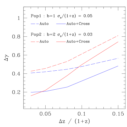
Figure 1: The gain from adding redshift-bins cross-correlations. Dashed lines show the expected 1-$\sigma$ constrains in $\gamma$ from the combined analysis of angular auto-correlation in photo-z bins spanning $0.4<z<1.4$, as a function of the bin width $\Delta z/(1+z)$ (see Table 1 for the corresponding total number of bins). Different colors correspond to different populations with bias and $\sigma_{z}$ as labeled. Solid lines show, for each population, the same study but also including all the cross-correlations between bins (and their complete covariance). For optimal bin widths $\Delta z\lesssim\sigma_{z}$ the gain from including cross-correlations is $\sim 2$ or better.

2.2.1 Radial selection functions

The radial selection functions $\phi_{i}$ in Eqs. (2,5,6) encode the probability to include a galaxy in the given redshift bin. Therefore, they are the product of the corresponding galaxy redshift distribution and a window function that depends on selection characteristics (e.g binning strategy),

$$\phi_{i}^{\alpha}(z)=\frac{dN_{\alpha}}{dz}\,W_{i}(z)$$ (9)

where $dN_{\alpha}/dz$ is given by Eq. (1). We include the fact that we are working with photo-z by using the following window function:

$$W_{i}(z)=\int{dz_{p}P(z|z_{p})W^{ph}_{i}(z_{p})},$$ (10)

where $z_{p}$ is the photometric redshift and $P(z|z_{p})$ is the probability of the true redshift to be $z$ if the photometric estimate is $z_{p}$. For our work we assume a top-hat selection $W^{ph}_{i}(z_{p})$ in photometric redshift and that $P(z|z_{p})$ is Gaussian with standard deviation $\sigma_{z}$. This leads to,

$$\phi^{\alpha}_{i}(z)\propto\frac{dN_{\alpha}}{dz}\left({\rm erf}\left[\frac{z_{p,max}-z}{\sqrt{2}\sigma^{\alpha}_{z}}\right]-{\rm erf}\left[\frac{z_{p,min}-z}{\sqrt{2}\sigma^{\alpha}_{z}}\right]\right)$$ (11)

where $z_{p,min}$ and $z_{p,max}$ are the (photometric) limits of each redshift bin considered and $\sigma^{\alpha}_{z}$ is the photometric redshift error of the given population $\alpha$ at the corresponding redshift.

2.2.2 Covariance matrix of angular power spectra

We assume that the overdensity field is given by a Gaussian distribution and therefore, the covariance between correlation $C_{\ell}^{i_{\alpha}j_{\beta}}$ and correlation $C_{\ell}^{p_{\alpha}q_{\beta}}$ is given by

$${\rm Cov}_{\ell,(i_{\alpha}j_{\beta})(p_{\mu}q_{\nu})}=\frac{C_{\ell}^{obs,i_{\alpha}p_{\mu}}C_{\ell}^{obs,j_{\beta}q_{\nu}}+C_{\ell}^{obs,i_{\alpha}q_{\nu}}C_{\ell}^{obs,j_{\beta}p_{\mu}}}{N(l)}$$ (12)

where $N(\ell)=(2\ell+1)\Delta\ell f_{sky}$ is the number of transverse modes at a given $\ell$ provided with a bin width $\Delta\ell$. We set $\Delta\ell=2/f_{sky}$, the typically chosen value to make Cov block-diagonal (?; ?). In this case, bins in $\ell$ are not correlated between them.

Therefore, for each $\ell$ bin, we define a matrix with $2N_{z}(2N_{z}+1)/2$ rows, where $N_{z}$ is the number of redshift bins, taking into account the covariances and cross-covariances of auto and cross-correlations between each population and among them. In order to include observational noise we add to the auto-correlations of each population in Eq. (12) a shot noise term

$$C_{\ell}^{obs,i_{\alpha}j_{\beta}}=C_{\ell}^{i_{\alpha}j_{\beta}}+\delta_{i_{\alpha}j_{\beta}}\frac{1}{\frac{N_{gal}(j_{\beta})}{\Delta\Omega}}$$ (13)

that depends on the number of galaxies per unit solid angle included in each radial bin. We define the $\chi$ assuming the observed power spectrum $C_{\ell}^{obs}$ corresponds to our fiducial cosmological model discussed in Sec. (2.3), while we call $C^{mod}_{\ell}$ the one corresponding to the cosmology being tested,

$$\chi^{2}=\sum_{\ell}\left(C_{\ell}^{obs}-C_{\ell}^{mod}\right)^{\dagger}{\rm Cov}_{\ell}^{-1}\left(C_{\ell}^{obs}-C_{\ell}^{mod}\right).$$ (14)

2.3 Cosmological model and growth history

Throughout the analyses, we assume the underlying cosmological model to be a flat $\Lambda$CDM with cosmological parameters $w=-1$, $h=0.7$, $n_{s}=0.95$, $\Omega_{m}=0.25$, $\Omega_{b}=0.045$ and $\sigma_{8}=0.8$. These parameters specify the cosmic history as well as the linear spectrum of fluctuations $P_{0}$. In turn, the growth rate can be well approximated by,

$$f(z)\equiv\Omega_{m}(z)^{\gamma}$$ (15)

and $\gamma=0.545$ for $\Lambda$CDM. Consistently with this we obtain the growth history as

$$D(z)\equiv\exp\left[-\int_{0}^{z}\frac{f(z)}{1+z}dz\right]$$ (16)

(where $D$ is normalized to unity today). The parameter $\gamma$ is usually employed as an effective way of characterizing modified gravity models that share the same cosmic history as GR but different growth history (?). Our fiducial model assumes the GR value $\gamma=0.545$. In order to forecast the constrains on $\gamma$ we consider it as a free parameter independent of redshift.

With these ingredients, we do a mock likelihood sampling in which we assume that the theoretical values for the correlations at the fiducial value of the parameters corresponds to the best fit position. The likelihood is based on the $\chi^{2}$ given in (14). In our case, we keep fixed all the parameters and only allow $\gamma$ to vary, and then we estimate 68% confidence limits of it. In the case in which we show constrains on $f\sigma_{8}$, we vary this quantity (that now depends on redshift, thus the number of fitting parameters is a function of the bin configuration), fixing the rest of parameters. The maximum $\ell$ considered in the analysis is $\ell_{max}=r(\bar{z}_{Survey})k_{max}\sim 220$ for $k_{max}=0.1\,{\it h}{\rm Mpc}^{-1}$, while for the largest scales we set $l_{min}=2$. We had to adapt CAMB$\_$sources in order to constrain $\gamma$ or $f\sigma_{8}$ using the same technique described in the Appendix A of ?.

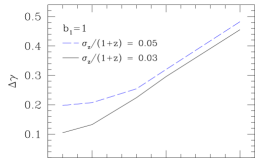
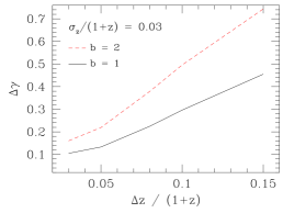
Figure 2: Dependence on photo-z (top panel) and bias (bottom panel) for a one-population constrains in $\gamma$, as a function of bin width (same as in Fig. 1). The panels show that lower $b$ and/or lower $\sigma_{z}$ yields better constrains in $\gamma$. This is hence a competing interplay because lower $b$ would correspond to a fainter sample with typically worse photometric errors. The dependence on bias seems however slightly stronger.

3 Results

In this section we discuss the constrains on the growth index, $\gamma$ defined in Eq. (15) as obtained for the different redshift bin configurations of Table 1. First of all, we study how well we can determine $\gamma$ using different single galaxy populations but including as observables also the cross correlation between bins (for a given single population). We also study how the constrains depend on the bias and in the photometric redshift accuracy of the different galaxy samples. Then, we study the precision achievable when one combines different tracers in the analysis and how this depends on bias, photo-z and in particular, the shot-noise level of the sample.

Lastly we discuss the constrains that we obtain when looking into the more standard $f(z)\sigma_{8}(z)$ as a function of redshift, and consider auto and cross-correlations of one or two galaxy samples.

3.1 Redshift-space distortions with a single photometric population

Let us first consider the constrains on the growth index using single photometric populations. Figure 1 shows the 1-$\sigma$ errors expected on $\gamma$ from a combined analysis of all the consecutive photometric redshift bins in the redshift range $0.4<z<1.4$ as a function of the bin width (i.e. each of the configurations detailed in Table 1).

In red we show the constrains on $\gamma$ corresponding to an LRG-type sample, with bias $b=2$ and a photometric redshift $\sigma_{z}/(1+z)=0.03$ (Pop2). Blue lines correspond to an unbiased population with $\sigma_{z}/(1+z)=0.05$ (Pop1).

Dashed lines correspond to the case in which we only use the auto-correlations in each redshift bin while solid lines corresponds to the full 2D analysis that includes all the cross-correlations in our vector of observables. Recall than in the first case the cross-correlations are included in the covariance matrix of the auto-correlations (but not as observables). We see that constrains from a full 2D analysis, including auto and cross-correlations are a factor $\sim 2$ or more better than those from using only auto-correlations.

From Fig.  1, it is clear that in all cases the bin configuration can be optimized, with the best results obtained when $\Delta z\sim\sigma_{z}$. In addition, there is a competing effect between $\sigma_{z}$ and bias. For broad bins ($\Delta z\gg\sigma_{z}$) the photo-z of the populations is masked in the projection and the bias dominates the $\gamma$ constrains. Smaller bias gives more relevance to RSD and better $\gamma$ constrains. As one decreases the bin width the population with better photo-z (typically the brighter, with higher bias), denoted Pop2, allows a more detailed account of radial modes improving the derived errors on $\gamma$ more rapidly than Pop1 until they become slightly better. This optimization is possible until one eventually reaches bin sizes comparable to the corresponding photo-z (what sets an “effective” width) and the constrains flatten out.

In Fig. 2, we study in more detail the dependence of constrains with respect to galaxy bias $b$ and photo-z accuracy. In the top panel of Fig. 2 we show standard deviation of the growth index, $\Delta\gamma$, fixing the sample bias to $b=1$ and allowing two values for photo-z accuracy. Red line represents a sample in which $\sigma_{z}/(1+z)=0.05$ while blue line has an error of $\sigma_{z}/(1+z)=0.03$. In both cases the constrain flattens once $\Delta z\sim\sigma_{z}$ and the optimal error improves roughly linearly with $\sigma_{z}$. The dependence on the linear galaxy bias, $b$, is shown in the bottom panel of Fig. 2 (for fixed $\sigma_{z}$). We see that the constrains degrade almost linearly with increasing bias (see also ?). As discussed before, this is because the lower the bias the larger the relative impact of RSD, which results in better constraints on $\gamma$.

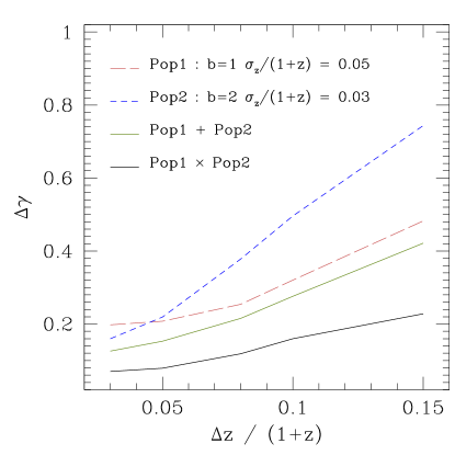
Figure 3: The gain from combining galaxy populations: Comparison of the 68% standard deviations in the growth index from single population analysis (dashed lines) with respect to the combined analysis of these two populations over the same field (black solid), using all the angular auto and cross-correlations. Remarkably the combination yields errors at least 2 times better than any of the single population cases. The solid green line corresponds to the combination of the two samples assuming they are independent (i.e. from different parts of the sky). As shown, the combination of correlated populations (same sky) yield stronger constrains than any other case.

In summary we have shown that using the whole 2D tomography (auto+cross correlations) allows considerable more precise measurements of $\gamma$, a factor of 2 or better once the bin width is optimal for the given sample. Hence in what follows we concentrate in full tomographic analysis.

3.2 Redshift-space distortions with 2 photometric populations

We now turn to an analysis combining two galaxy populations as two different tracers of matter. In Figure 3 we compare the constrains from single tracers with respect to the combination of both. As before the populations used in the comparison correspond to $b=1$ and $\sigma_{z}/(1+z)=0.05$ (Pop 1) and a population with $b=2$ and $\sigma_{z}/(1+z)=0.03$ (Pop 2). Their respective constrains in $\gamma$ are the dashed red and blue lines (same as solid lines in Fig. 1).

If we combine both tracers and their cross-correlation in the same analysis we obtain the constrains given by black solid line, notably a factor of $2-3$ better compared to the optimal single population configuration.

In order to understand how much of this gain is due to “sample variance cancellation”, in analogy to the idea put forward in ?, we also considered combining the two samples assuming they are located in different parts of the sky (and hence un-correlated). We call this case Pop1+Pop2 in Fig. 3 (solid green line). In such scenario the total volume sampled is the sum of the volumes sampled by each population (in our case, two times the full volume of DES). This explains the gain with respect to the single population analysis. Nonetheless, the “same sky” case Pop1 $\times$ Pop2 (where cosmic variance is sampled twice) still yields better constrains, a factor of $\sim 1.5-2$, even though the area has not increased w.r.t. Pop1 or Pop2 alone.

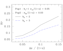
Figure 4: Dependence on bias. Increasing the bias difference between the samples improves the constrains on $\gamma$. The solid black line corresponds to the combination Pop1 $\times$ Pop2 of a highly biased sample such as LRGs (Pop2) with an unbiased one (Pop1), while the blue dashed to cluster-like bias tracer as Population 2.

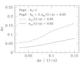
Figure 5: Dependence on photometric redshift error. Similar to Fig. 4 but now changing the photo-z of the unbiased sample (Pop1) for a fixed 2nd population. The error on $\gamma$ depend roughly linear with $\sigma_{z}/(1+z)$ for optimal bin widths.

In all, the total gain of a full 2D study with two populations (including all auto and cross correlations in the range $0.4<z<1.4$) w.r.t. the more standard analysis with a single population and only the auto-correlations in redshift bins (dashed lines of Fig. 1) can reach a factor of $\sim 5$.

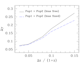
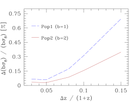
Figure 6: Bias free case: If the biases of the samples are free parameters to marginalize over we find that constrains on $\gamma$ degrade only slightly compared with the bias fixed case. In particular for the thinner redshift bins configurations. This is because biases are determined with relative errors smaller than 1% (bottom panel).

As a next step we show how the combined analysis of two tracers depends on the relative difference on the bias and photo-z errors of the populations. In Fig. 4 we keep Pop1 fix (with $b=1$ and $\sigma_{z}/(1+z)=0.05$) and we vary the bias of Pop2 from $b=2$ (LRG type bias) to $b=3$ (galaxy clustering like). We keep $\sigma_{z}/(1+z)=0.03$ fixed for Pop2. As expected, increasing the bias difference between the samples improves the constrains on $\gamma$ in a roughly linear way.

If we now have an unbiased tracer and a highly biased one with $b=3$, while both tracers have the same $\sigma_{z}/(1+z)=0.03$ we obtain constrains given by the black line in Fig. 5. Those constrains are better than the case in which the unbiased galaxies photo-z is worse, $\sigma_{z}/(1+z)=0.05$ (given by the dashed blue line). Therefore, if we determine photometric redshifts of the unbiased galaxies with higher accuracy we will be able to measure the growth rate with higher precision.

One caveat so far is that we have always assumed that biases are perfectly known (bias fixed). Hence, in the top panel of Fig. 6 we show how the constrains on $\gamma$ change if we instead consider them as free parameters and marginalize over. We see that the difference is very small, in particular once the bin configuration is optimal. The reason for this is clear from the bottom panel that shows the relative error obtained for the bias of each sample in the bias free case. Because the bias is so well determined (sub-percent) the marginalization over them does not impact the error on $\gamma$.

3.2.1 The impact of photo-z uncertainties

The constrains on growth of structure presented in this paper rely to a good extent on cross-correlations between redshift bins, in turn largely determined by the overlap of the corresponding redshift distributions. So far we have assume a perfect knowledge of these distributions, given by Eq. (11). However in a more realistic scenario the distribution of photometric errors, and hence redshift distributions, will be known only up to some uncertainty. In this section we investigate the impact of such uncertainties in the constrainig power on growth rate by marginalizing over redshift distributions.

For concreteness we focus in a case with only two redshift bins with $z_{mean}=\{0.78,0.96\}$ and width $\Delta z/(1+z)=0.1$). In our framework redshift distributions are characterized by a width, given by $\sigma_{z}$ in Eq. (11), and set of minimum and maximum values for the photometric top-hat selection that determine the mean redshift $z_{mean}=(z_{p,min}+z_{p,max})/2$. Thus, to marginalize over miss-estimations of photometric errors, the “width” of $n(z)$, we vary $\sigma_{z}$. To marginalize over the “mean redshift” of $n(z)$, we shift both $z_{p,min}$ and $z_{p,max}$ by the same amount. This procedure automatically changes either the width or the location of the underlying redshift distribution. Effectively, it also marginalizes over the amount of bin-overlap. In what follows we do not put priors on any parameter.

Figure 7 shows the $1-\sigma$ contours of the growth rate index $\gamma$, the mean redshift of the second bin and the width of the photometric error at this bin for the bright population with $b=2$ and $\sigma_{z}/(1+z_{mean})=0.03$ (Pop 2). For this first case we have choosen to set $z^{bin1}_{p,max}=z_{p,min}^{bin2}$ as we marginalized over mean redshift of bin 2. This means that we are also changing the width and location of the redshift distribution of bin 1 (while the amount of bin-overlap is set by the nuisance variable $\sigma_{z}^{bin2}$).

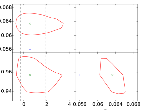
Figure 7: The impact of photo-z uncertainties on growth rate measurements: We considered a case with only two redshift bins, with fiducial $z_{mean}=\{0.78,0.96\}$ for a population with $b=2$ and $\sigma_{z}/(1+z)=0.03$ where the location ($z_{mean}$) and width ($\sigma_{z}$) of the redshift distribution of the second bin are free parameters (in addition to $\gamma$). The figure shows the 68% confidence regions for $\gamma$, $z_{mean}$ and $\sigma_{z}$. Black dashed lines enclose the $1-\sigma$ region when $\gamma$ is the only free parameter. Blue “+” markers correspond to fiducial values while green “x” markers correspond to the best fit value after marginalizing over the remaining parameter. The marginalized error in $\gamma$ increases by $10\%$ with respect to perfectly known redshift distributions (dashed lines). In turn the best-fit $\gamma$ is unbiased (see text for further cases).

From Fig. 7, we find that marginalizing over $z_{mean}$ and $\sigma_{z}$ increases the best-fit bin width above the fiducial value by $\%10$ but it does not bias the recovered growth rate index (neither the mean redshift). The error on $\gamma$ increases by about $10\%$ when marginalizing over the $z_{mean}$ and $\sigma_{z}$ of bin 2, compared with the case with fixed $z_{mean}$ and $\sigma_{z}$ (represented by dashed lines in Fig. 7). In turn the marginalization shows that $\sigma_{z}$ and $z_{mean}$ are slightly correlated (bottom right panel of Fig. 7). We performed the same marginalization for the population with $b=1$ and $\sigma_{z}/(1+z)=0.05$ (Pop 1), finding similar conclusions ($\gamma$ is recovered unbiased, with an error $14\%$ worse).

We also considered what happens if we do not keep both bins sharing the same boundary in photo-z space. In this case the redshift distribution of bin 1 is kept totally fixed through marginalization of $n^{bin2}(z)$ and the bin-overlap is changed by both $z_{mean}$ and $\sigma_{z}$ of bin 2. In this case we find a smaller correlation between $z_{mean}$ and $\sigma_{z}$ and also a smaller marginalized error on $z_{mean}$. The marginalized error on $\gamma$ increases by $9\%$ when considering Pop1 and only $\%6$ for Pop2, while the best-fit value is always recovered un-biased.

A full analysis on how to optimize and marginalize the photo-z uncertainties using more realistic photometric errors is beyond the scope of this paper. But the results presented in this section, and Fig. 7, indicates that it is possible to account for such uncertainties without a major loss in constraining power on growth rate measurements.

3.2.2 The impact of shot-noise

One strong limitation when it comes to implementing the “multiple tracers” technique in real spectroscopic data is the need to have all the galaxy samples well above the shot-noise limit (at the same time as having the largest possible bias difference), see for instance ?. This is cumbersome because spectroscopic data is typically sampled at a rate only slightly above the shot-noise (to maximize the area) and for pre-determined galaxy samples (e.g LRGs, CMASS). In a photometric survey these aspects change radically because there is no pre-selection (beyond some flux limits) and the number of sampled galaxies is typically very large (at the expense of course of poor redshift resolution). Therefore is interesting to investigate if the overall density of the samples have any impact in our results.

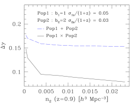
Figure 8: The impact of shot noise: We consider the combined analysis of two populations in a redshift bin configuration of $\Delta_{z}/(1+z)=0.05$ and show how constrains on $\gamma$ depend on the (shot) noise level of the more biased population (typically the brighter, less abundant sample). Constrains are almost un-affected unless the density drops by an order of magnitude or more compared to the one of Pop1 ($n_{2}=0.023\,{\it h}^{3}\,{\rm Mpc}^{-3}$).

Figure 8 shows the constrain in $\gamma$ for the combination of two samples, one unbiased population with $\sigma_{z}/(1+z)=0.05$ and a population with $b=2$ and $\sigma_{z}/(1+z)=0.03$. We keep the number density for the unbiased population as $n(z=0.9)=1.8\times 10^{-2}\,{\it h}^{3}{\rm Mpc}^{3}$ while we vary the number density of the second (typically brighter) sample. The solid black line corresponds to the case in which both populations are correlated (same sky) and the dashed blue line to different areas. In both scenarios we see that decreasing the number density of the second population does not impact the error on $\gamma$ unless one degrades it by an order of magnitude or more (below $n(z=0.9)\sim 3.0\cdot 10^{-3}$). Above this value, the error is mostly controlled by the tracer with lower bias.

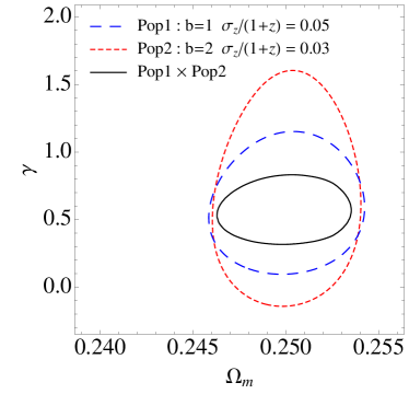
Figure 9: Marginalizing over the shape of P(k) : Contour plot of the posterior joint distribution when we consider both $\gamma$ and $\Omega_{m}$ as nuisance parameters. We find no significant degeneracies. The error on $\gamma$ degrade $35\%$ for Pop1, $16\%$ for Pop2 and only $6\%$ for Pop1$\times$Pop2. These results corresponds to a combined analysis of 6 bins with $\Delta z/(1+z)=0.1$.

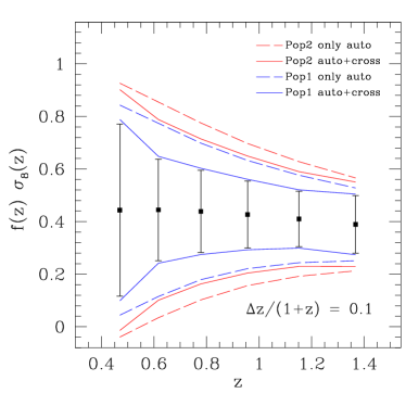
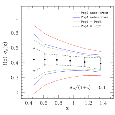
Figure 10: Constrains on $f\sigma_{8}$: derived at different redshift bins, for a bin configuration of $\Delta z/(1+z)=0.1$. The left panel focuses on one population only fits, and the gain from using auto+cross correlations among all redshift bins as observables instead of just the auto-correlations. The right panel stresses instead the gain from combining two populations (through their auto and cross-correlations) either in different patches of the sky (Pop1$+$Pop2) or the same (Pop1$\times$Pop2). In all cases Pop1 refers to a galaxy population with $b=1$ and $\sigma_{z}/(1+z)=0.05$ and Pop2 to $b=2$ and $\sigma_{z}/(1+z)=0.03$. The covariance among the derived errors on $f(z)\times\sigma_{8}(z)$ is taken into account in the fit. Our results show that by using RSD with two tracers a DES-like photometric survey can place $\sim 15\%$ constrains in the evolution of $f\sigma_{8}$ for several bins in $z\gtrsim 0.8$ (with errors almost uncorrelated between bins, see text for details).

3.2.3 Marginalizing over Power spectrum shape

In the analysis presented so far, we have assumed a perfect knowledge on the shape of the matter power spectrum and hence of the underlying cosmological parameters. However it is important to explore possible degeneracies between the parameter we base on for RSD, namely $\gamma$, and other cosmological ones. While we leave a full exploration of degeneracies for a follow-up paper we now study the impact of varying the shape of the power spectrum in addition to $\gamma$. We do this by considering the matter density $\Omega_{m}$ as a nuisance parameter to marginalize over. By doing so, we are mostly studying the effect of the matter power spectrum shape in the analysis.

For concreteness we focused on the binning configuration with $\Delta z/(1+z)=0.1$ (6 bins). Figure 9 shows the contour plots of the posterior distribution in the $\Omega_{m}-\gamma$ for Pop1 (unbiased with bad photo-z), Pop2 (biased with good photo-z) and Pop1$\times$ Pop2. We find that there are no significant degeneracies and $\Omega_{m}$ is determined with quite good precision.

Then, if we marginalize over $\Omega_{m}$, we see that the errors on $\gamma$ degrade a $16\%$ for an unbiased population, a $35\%$ for the biased one while the effect when we cross correlate both populations is only a $6\%$ worse error on $\gamma$. Therefore, the conclusions obtained in previous sections are still valid, even if we allow the shape of the matter power spectrum to change.

3.3 Constraining the redshift evolution of the Growth Rate of Structure

So far we have used the combined analysis of all the redshift bins to constrain one global parameter, namely the growth rate index $\gamma$ in Eq. (15). We now turn into constraining $f(z)\sigma_{8}(z)$ itself, as a function of redshift. We use a redshift bin configuration given by $\Delta z/(1+z)=0.1$, in the photometric range $0.4<z<1.4$. This configuration consist of 6 bins, and hence we fit $f(z)\sigma_{8}(z)$ evaluated at the mean of these bins. These $f\sigma_{8}$ values are of course correlated, and we include the proper covariance among the measurements (i.e. we do a global fit to the 6 values simultaneously).

In the left panel of Fig. 10 we focus on the gain from adding cross-correlations among the bins, and show the constrain on $f\sigma_{8}$ for a single unbiased population with photometric redshift of $\sigma_{z}=0.05$ (Pop 1, in blue) and also for a single tracer with bias $b=2$ and $\sigma_{z}=0.03$ (Pop 2, in red). Dashed lines corresponds to using only auto-correlations and solid to including also all the redshift bins cross-correlations to the observables. The trend for the errors when we only use auto-correlations are similar to the ones observed in Fig. 8 of ?. Although in detail we are using different widths for our redshift bins, and we use $C_{\ell}$ while they used angular correlation functions, $w(\theta)$.

As in Sec. 3.1 there is a gain from the addition of cross-correlations, which is now split across the bins (i.e. $20-30\%$ for Pop1 in each of the 6 bins, and a bit less for Pop2).

In turn, the right panel of Fig. 10 focuses in the gain from combining the two tracers (and using both auto and cross correlations among redshift bins, as in Sec. 3.2). Here the solid lines correspond to the single population cases discussed above, while the black short-dashed line to the combined analysis assuming these populations are correlated (same sky). For completeness, the dashed green line is the result when these two samples are assumed independent. Again, there is a factor of $\sim 2.5$ to be gained by combining galaxy samples as opposed to only the unbiased sample.

If we compare our predictions to measurements from spectroscopic surveys like VIPERS (?) with constrains $f\sigma_{8}(z=0.8)=0.47\pm 0.08$ or WiggleZ (?) where $f\sigma_{8}(z=0.76)=0.38\pm 0.04$ we find that DES can achieve the same level of errors ($\sim 15\%$) in determining the growth of structure but extending the constrains beyond redshift of unity. This is quite unique and interesting as there is, to our knowledge, no other spectroscopic survey expected to provide such measurements in the medium term future (before ESA/Euclid or DESI).

3.3.1 Impact of unknown redshift distributions

In this section, we investigate the consequences of not having a perfect knowledge of the redshift distributions used to project the 3D clustering into tomographic bins. For concreteness we do this by investigating how the error on $f\sigma_{8}$ resulting from a single bin at $z=1.15$ change when we also vary the assumed underlying redshift distribution (within the binning configuration of $\Delta z/(1+z)=0.1$). We note that in doing this we consider the full covariance with adjacent bins while the explored parameter space consist of 3 values of $f(z)\sigma_{8}(z)$ (at $z=1.05,1.15,1.36$) and either the mean or the width of $N(z)$ for the central bin at $z=1.15$.

We first concentrated in marginalized over the mean redshift of the assumed $N(z)$ for the central bin assuming a flat prior of $3\%$ around $z_{mean}=1.15$. We have repeated this for all the cases explored in Fig. 10, namely we consider populations 1 and 2 individually and then the same sky and different sky combinations of both populations. We have not found significant changes with respect to the results in previous sections finding differences smaller than $1\%$ for the cases with individual populations and less than $5\%$ for the case in which we combine the two populations.

Then, we marginalize over photometric errors and we find differences smaller than $1\%$ in the recovered constrains in $f(z)\sigma_{8}(z)$ with respect to the case in which we assume perfect knowledge of the redshift distributions. For concreteness we did this cross-check for the case Pop1$\times$Pop2 in last two redshift bins shown in Fig. 10.

3.4 The case of high-photometric accuracy

In the previous sections, we have focused in galaxy surveys with broad-band photometry for which the typical photometric error achieved is of the order $0.1$ depending on galaxy sample and redshift. We now turn to narrow-band photometric surveys such as the ongoing PAU or J-PAS Surveys (?; ?; ?; ?). These surveys are characterized by a combination of tens of narrow band (NB) filters ($\sim 100\mbox{\AA}$) and few standard broad bands (BB) in the optical range. In the concrete case of PAU the NB filters are $40$ in total ranging from $\sim 4400\mbox{\AA}$ to $\sim 8600\mbox{\AA}$ that will perform as a low resolution spectrograph. With the current survey strategy, it will obtain accurate photometric redshifts for galaxies down to $i_{AB}\sim 22.5$ for which the typical redshift accuracy will be $\simeq 0.003(1+z)$ (or $10{\it h}^{-1}\,{\rm Mpc}$). This scenario then resembles quite closely a purely spectroscopic survey (?). However the expected density of this sample is $\sim 10000$ galaxies per ${\rm deg}^{2}$, much denser than any spectroscopic surveys to the same depth.

We do not aim here at giving a forecast for PAU but rather at investigating the issue of combining samples with high-photometric accuracy. Hence we will assume the same overall redshift distribution as in Sec. 2.1 but consider only a total $50\times 10^{6}$ galaxies within $5000$ deg². This is in broad agreement with PAU specifications (see ? and ? for further details).

We again study two populations, one corresponding to the main sample with bias $b=1$ and another to the LRG sample with $b=2$, both with a very good photometric accuracy of $\sigma_{z}/(1+z)=0.003$. We consider a set of 21 narrow redshift bins of width $\Delta z=0.003(1+z)$ concentrated in $0.94<z<1.06$ (hence we are only looking at a portion of the survey redshift range).

The error on $\gamma$ are given in Table 2, for both the new narrow-band and the broad-band samples discussed previously. For a single population, this table shows that a factor of $\sim 10$ better $\sigma_{z}$ yields a factor of $\sim 10$ gain in constraining power. The improvement in $\gamma$ seems to increase linear with the improvement in $\sigma_{z}$.

${\rm Population}$	b	$\sigma_{z}/(1+z)$	${\rm Auto}$	${\rm Auto+Cross}$
Broad Band (BB)
${\rm Pop1}$	1	0.05	0.809	0.564
${\rm Pop2}$	2	0.03	0.826	0.447
${\rm Pop1\times Pop2}$	-	-	-	0.35
${\rm Pop1+Pop2}$	-	-	-	0.36
Narrow Band (NB)
${\rm Pop1}$	1	0.003	0.047	0.027
${\rm Pop2}$	2	0.003	0.088	0.040
${\rm Pop1\times Pop2}$	-	-	-	0.016
${\rm Pop1+Pop2}$	-	-	-	0.023

Table 2: Error in the growth rate $\gamma$ from a combination of $21$ narrow bins in the range $0.94<z<1.06$. The 4 top entries correspond to a Survey with Broad-Band (BB) filters: Pop1-BB assumes $b=1$ and $\sigma_{z}/(1+z)=0.05$ (“main sample”) while Pop2-BB has $b=2$ and $\sigma_{z}/(1+z)=0.03$ (“LRG sample”). The 4 bottom entries correspond to a Survey with Narrow-Band (NB) filters. Here Pop1 and Pop2 have the same bias as the BB case but much precise photo-z, both with $\sigma_{z}/(1+z)=0.003$.

After combining the two populations, we see that the errors in $\gamma$ for the broad-band case is similar if samples cover the same region of sky (${\rm Pop1\times Pop2}$) or different regions (${\rm Pop1+Pop2}$). This is because the redshift range considered ($0.94<z<1.06$) is too narrow compared to $\sigma_{z}$ and the cosmic variance cancelation can not take place. Instead, for the narrow band surveys we find a $43\%$ improvement for the case ${\rm Pop1\times Pop2}$ with respect to ${\rm Pop1+Pop2}$. For the same sky case, the final error is $\Delta\gamma\simeq 0.0163\times(5000\,{\rm deg}^{2}/{\rm Area})^{1/2}$, in such a way that even a moderate survey of $250\,{\rm deg}^{2}$ could achieve $\Delta\gamma\sim 0.07$. In that same narrow redshift range, DES yields an error 5 times worse with 20 times better area (but note that in the case of small areas we could be limited by the $\ell_{min}$, the largest scales available).

4 Conclusions

We have studied how measurement of redshift-space distortions (RSD) in wide field photometric surveys produce constrains on the growth of structure, in the linear regime. We focused in survey specifications similar to those of the ongoing DES or PanSTARRS, that is, covering about $1/8$ of sky up to $z\sim 1.4$, and targeting galaxy samples with photometric redshift accuracies of $0.03-0.05(1+z)$ (and hundred of million galaxies prior to sample selection). We also show results for ongoing photometric surveys, such as PAU and J-PAS, that have a much better photometric accuracy.

First, we have found that for a single population we can reduce the errors in half by including all the cross-correlations between radial shells in the analysis. This is because one includes large scale radial information that was missed when only considering the auto-correlations of each bin. The final constraining power depends on the details of the population under consideration, in particular the bias and the photometric accuracy. Less bias gives more relative importance to RSD in the clustering amplitudes. In turn, better photo-z allows for narrower binning in the analysis and more radial information. We find that the $\gamma$ constrains depend roughly linearly in both bias or $\sigma_{z}$. This means that for 10 times better photo-z errors, such as in PAU, we can improve by 10 the cosmological constrains.

Typically less bias implies a fainter sample, with worse photo-z, therefore these quantities compete in determining the optimal sample. Furthermore we find that optimal constrains are achieved for bin configurations such that $\Delta z\sim\sigma_{z}$. Although the optimal errors depend on the details of the galaxy sample and binning strategy, the gains from adding cross-correlations are very robust in front of these variations.

In order to avoid sample variance, we have also considered what happens if we combine the measurement of RSD using two different tracers. This is motivated by the idea put forward in ? for the case of spectroscopic (hence 3D) redshift surveys, where the over-sampling of (radial + transverse) modes allows a much better precision in growth rate constrains, as long as samples are in the low shot-noise limit. Combining auto and cross angular correlations in redshift bins, we find that if we assume that both tracers are independent, which corresponds to samples from different regions on the sky, the constrains on the growth of structure parameters improve a 30-50% (due to the fact that one has doubled the area). Remarkably if we consider that the populations are not independent, i.e., they trace the same field region, we find an overall improvement of $\sim 2-3$ with respect to single populations when constraining $\gamma$. This means that there is a large potential gain when sampling the same modes more than once.

Translating into actual constrains this implies that a DES-like photometric survey should be able to measure the growth rate of structure $\gamma$ to an accuracy of $5-10\%$ from the combination of two populations and all the auto+cross correlations in the range $0.4<z<1.4$ (see Fig. 1). Even though these values correspond to a survey of $5000{\rm deg}^{2}$ ($f_{sky}=0.125$) they should scale as $f_{sky}^{-1/2}$ for a different area, given our assumptions for the covariance in Eq. (12).

In Fig. 8, we have shown that constrains weaken once one of the populations enter a shot-noise dominated regime, as is typical of spectroscopic samples. However one needs to dilute over 10 times the number densities for a photometric survey, such as DES, for this to happen. Thus, as shown in Section 3.4, by improving on photo-z accuracy without much lost of completeness, a photometric sample can in fact outperform a diluted spectroscopic version with similar depth and area (see also ?).

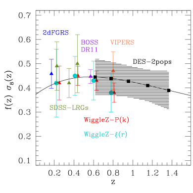
Figure 11: Combined constrains in the evolution of the growth rate of structure from spectroscopic data, 2dFGRS, SDSS-LRGs, Wiggle-Z, VIPERS and BOSS (see text for details), and forecasted for DES using two photometric populations (same as in Fig. 8). The addition of DES (shaded area) allows to trace the growth rate of structure all the way to $z\sim 1.4$.

In this paper we focused on large angular scales where the approximation of linear and deterministic bias and linear RSD should hold (see for instance ?). Although we set $\ell_{max}\sim 200$, much of the constraining power in our results, given the typical size of our redshift bins, comes from larger scales, $\ell\lesssim 40$. Yet, a more realistic assessment of these aspects will need to resort to numerical simulations. We leave this for future work.

Lastly, we also investigated what constrains can be placed with this method in the evolution of the growth rate of structure, $f(z)\times\sigma_{8}(z)$. We found that binning two DES populations into $6$ bins in the range $0.4<z<1.4$ yields constrains on $f(z)\times\sigma_{8}(z)$ of $\sim 15\%$ for each bin above $z\sim 0.6$. This is shown in Fig. 11. That case corresponded to bin widths larger than the photometric errors of the samples, which may not be optimal but yield constrains almost uncorrelated between bins ($\rho_{ij}\sim-0.05$). A narrower binning, $\Delta z/(1+z)=0.05$ leads to better constrains per bin, $\Delta(f\sigma_{8})\sim 10\%$, at the expense of more correlation between bins, $0.2<\rho_{ij}<0.65$.

In addition to the DES forecast (shadowed region) we over-plot in Fig. 11 current constrain from spectroscopic surveys, 2dFGRS (?), LRG’s from SDSS (? and ?), WiggleZ either from power spectrum (?) or correlation function (?), and the recent VIPERS, (?) and BOSS results (?). Note that these values are not expected to improve radically in the near future. This implies that DES will be able to add quite competitive constrains in a redshift regime unexplored otherwise with spectroscopic surveys (i.e. $z\gtrsim 1$), yielding a valuable redshift leverage for understanding the nature of dark energy and cosmic acceleration through the growth of structure.

References

- [Asorey et al. ¡2012¿] Asorey J., Crocce M, Gaztañaga E., Lewis A., 2012, MNRAS 427, 1891
- [Banerji et al. ¡2008¿] Banerji M., Abdalla F. B., Lahav O., Lin, H., 2008, MNRAS 386, 1219
- [Benitez et al. ¡2009¿] Benitez N., et al., 2009, ApJ 691, 241
- [Benjamin et al. ¡2013¿] Benitez N., et al., 2013, MNRAS 431, 1547
- [Blake et al. ¡2007¿] Blake C., Collister A., Bridle S., Lahav O., 2007, MNRAS 374, 1527
- [Blake et al. ¡2011¿] Blake C., et al., 2011 ,MNRAS 415, 2876B
- [Bonvin C., Durrer R.¡2011¿] Bonvin C., Durrer R., 2011, Phys. Rev. D 84, 063505
- [Cabré et al.¡2007¿] Cabré A., Fosalba P., Gaztañaga E., Manera M., 2007, MNRAS 381, 1347
- [Cabré & Gaztañaga ¡2009¿] Cabré A., Gaztañaga E., 2009, MNRAS 393 ,1183
- [Cai & Bernstein ¡2012¿] Cai Y. C., Bernstein G., 2012, MNRAS 422, 1045
- [Castander et al. ¡2012¿] Castander F. J., et al., 2012, Proceedings of the SPIE 8446, 84466D
- [Challinor & Lewis¡2011¿] Challinor A., Lewis A., 2011, Phys. Rev. D 84, 043516
- [Crocce, Cabré, & Gaztañaga¡2011¿] Crocce M., Cabré A., Gaztañaga E., 2011, MNRAS 414, 329
- [Contreras et al. ¡2013¿] Contreras C, et al., 2013, MNRAS 430, 924
- [Crocce et al.¡2011¿] Crocce M., Gaztañaga E., Cabré A., Carnero A., Sánchez E., 2011, MNRAS 417, 2577
- [de la Torre et al.¡2013¿] de la Torre S., Guzzo L., Peacock J. A., et al., 2013, A&A submitted, e-print arXiv:1303.2622
- [de Putter R., Doré O. & Takada M.¡2013¿] de Putter R., Doré O. & Takada M., 2013, [eprint arXiv::1308.6070]
- [Fisher, Scharf & Lahav ¡1994¿] Fisher K. B., Scharf C. A., Lahav O., 1994, MNRAS 266, 219
- [Gaztañaga et al. ¡2012¿] Gaztañaga E., Eriksen M., Crocce M., Castander F. J., Fosalba P., Marti P., Miquel R., Cabré A., 2012, MNRAS 422, 2904
- [Gil-Marín et al. ¡2010¿] Gil-Marín H., Wagner C., Verde L., Jimenez R., Heavens A. F., 2010, MNRAS 407, 772
- [Guzzo et al. ¡2009¿] Guzzo L., et al., 2009, Nature 451 ,451
- [Hamilton ¡1998¿] Hamilton A. J. S., 1998,“Linear redshift distortions: A review”, in “The Evolving Universe”, ed. D. Hamilton, pp. 185-275 (Kluwer Academic, 1998) [eprint arXiv: astro-ph/9708102]
- [Kaiser¡1987¿] Kaiser N., 1987, MNRAS, 227, 1
- [Kazin et al. ¡2013¿] Kazin E. A., et al., 2013, MNRAS, 435, 64
- [Kirk et al.¡2013¿] Kirk D., Lahav O., Bridle S., Jouvel S., Abdalla F., Frieman J., 2013, [eprint arXiv:1307.8062]
- [Lewis et al. ¡2000¿] Lewis A., Challinor A., Lasenby A., 2000, ApJ 538, 473
- [Lewis & Challinor. ¡2007¿] Lewis A., Challinor A. 2007 Phys. Rev. D 76, 083005
- [Limber¡1954¿] Limber D. N., 1954, ApJ 119, 655
- [Linder¡2005¿] Linder, E. V. 2005, Phys. Rev. D 72, 043529
- [LoVerde & Afshordi ¡2008¿] LoVerde M., Afshordi N., Phys. Rev. D, 78, 123506 (2008)
- [McDonald & Seljak ¡2009¿] McDonald P., Seljak U., 2009, JCAP 0901, 007
- [Montanari & Durrer ¡2012¿] Montanari F., Durrer R., 2012, Phys. Rev. D 86, 063503
- [Newman ¡2008¿] Newman J. A., 2008, ApJ 684, 88
- [Nock, Percival,& Ross¡2010¿] Nock K., Percival W. J., Ross A. J., 2010, MNRAS 407, 520
- [Okumura et al. ¡2008¿] Okumura T., Matsubara T., Eisenstein D. J., Kayo I., Hikage C., Szalay A. S., Schneider D.P., 2008, ApJ 676, 889
- [Padmanabhan et al. ¡2007¿] Padmanabhan N., et al., 2007, MNRAS 378, 852
- [Percival et al. ¡2004¿] Percival W., et al., 2004, MNRAS 353, 1201
- [Reid et al. ¡2012¿] Reid B., et al., 2012, MNRAS 426, 2719
- [Ross et al.¡2011¿] Ross A. J., Percival W. J., Crocce M., Cabré A., Gaztañaga E., 2011, MNRAS 415, 2193
- [Samushia et al. ¡2014¿] Samushia L., et al., 2014, MNRAS 439, 3504
- [Taylor et al. ¡2013¿] Taylor K., et al., 2013, arXiv:1301.4175
- [Tegmark et al. ¡2006¿] Tegmark M. et al., 2006, Phys. Rev D 74, 123507
- [Abbott et al. ¡2005¿] The Dark Energy Survey Collaboration, White Paper submitted to the Dark Energy Task Force, [eprint arXiv::astro-ph/0510346]
- [Thomas, Abdalla & Lahav¡2011¿] Thomas, S. A., Abdalla, F. B., Lahav, O. 2011, MNRAS 412, 1669
- [White, Song & Percival ¡2009¿] White M., Song Y-S., Percival W. J., 2009, MNRAS, 397, 1348