Higgs couplings beyond the Standard Model

Abstract

We consider the Higgs boson decay processes and its production and provide a parameterisation tailored for testing models of new physics. The choice of a particular parameterisation depends on a non-obvious balance of quantity and quality of the available experimental data, envisaged purpose for the parameterisation and degree of model independence. At present only simple parameterisations with a limited number of fit parameters can be performed, but this situation will improve with the forthcoming experimental LHC data. It is therefore important that different approaches are considered and that the most detailed information is made available to allow testing the different aspects of the Higgs boson physics and the possible hints beyond the Standard Model.

I Higgs coupling parameterisations

Since the discovery of the Higgs boson last year by both ATLAS and CMS collaboration, it is clear that the study of its couplings is likely to give valuable information on the nature of the electroweak symmetry breaking and eventually to probe New Physics scenarios. Indeed, many of the currently studied BSM (Beyond the Standard Model) models can generically lead to deviations in the Higgs couplings, allowing for a constraint complementary to the direct searches for extra particles. However, to achieve such a goal, one must first make contact between the theory side (that is, the large amount of BSM models) and the experimental one (which are the results presented by the collaborations), and this implies the choice of a parameterisation.

From the experimental point of view it makes sense to just parameterise Higgs physics in terms of observed quantities such as branching ratios and cross-sections. This is for example the case of the parameterisation proposed in Ref. Group et al. (2012), where the relevant cross-sections and partial decay widths are multiplied by a suitable factor. The advantage of such an approach is its simple link to the experimentally measured quantities. On the other hand, with such a choice, correlations among the different parameters are not explicit, in particular between tree level and loop induced observables. For example, a modification of the couplings to $W$ bosons and top will also affect the loop-level couplings for the Higgs production via the gluon channel or the Higgs decay into two photons. Instead, we propose thus in Cacciapaglia et al. (2013) a parameterisation where the contribution of loops of New Physics to the $H\to gg$ and $H\to\gamma\gamma$ modes is explicitly disentangled from the modification of tree level couplings.

We must point that out that many studies have also been carried out relying on an effective field theory approach (Bonnet et al. (2012, 2012); Corbett et al. (2012); Espinosa et al. (2012a, b) ). While this approach has the important feature of allowing a full treatment of the radiative corrections (see Passarino (2013)), it often relies on a large set of parameters, for which the current experimental accuracy is still lacking a bit behind. A similar study has also been recently carried out in Belanger et al. (2013).

II Using experimental Higgs results

In order to use the latest data from ATLAS and CMS collaboration (atl ; cms ), one has to define the compatibility of a given model with data. The first approach is to use a $\chi^{2}$ test based on the signal strength $\mu$ which is simply the cross-section for $pp\to H\to XX$ normalised to the Standard Model expectation. Thus the $\chi^{2}$ reads

$$\chi^{2}(\kappa)=\sum_{i}\left(\frac{\hat{\mu}_{i}-\mu_{i}(\kappa)}{\sigma_{i}}\right)^{2},$$ (1)

where $\hat{\mu}$ is the best fit reported by the experiment, $\mu(\kappa)$ the prediction of the model on the parameter point $\kappa$, $\sigma$ the uncertainty, and $i$ runs on all subchannels of each experiment. Then this $\chi^{2}(\kappa)$ is compared to a standard $\chi^{2}$ distribution with $n$ degrees of freedom, where $n$ is the number of subchannels, in order to determine if the model is excluded or not. However this method suffers from a few shortcomings : first the $\mu_{i}(\kappa)$ does not correspond to the inclusive cross-section, but to the exclusive one. For instance the $H\to\gamma\gamma$ decay mode in ATLAS is divided into 11 subchannels, which amount to as many exclusive cross-sections. To compute exclusive cross-sections, one needs the experimental fractions per mode $\zeta_{i}^{p}$, or equivalently the efficiencies :

$$\mu_{i}^{XX}=\sum_{p}\zeta_{i}^{p}\mu_{p}^{XX},$$ (2)

where $\zeta_{i}^{p}$ represent the SM fraction of the production mode $p$ among all production modes in the subchannel $i$, and $\mu_{p}^{XX}$ the signal strength of that specific production mode in the final state $XX$. Although the $\zeta_{i}^{p}$ are computed by the collaborations themselves, there are not always publicly available. Another inconvenient raised by eq. 1 is that in adding all subchannels together we implicitly assume that they are not correlated. While this is the case of statistical uncertainty it is certainly not true for systematical uncertainty, let alone theory uncertainty.

II.1 Improved $\chi^{2}$ method

There exists nevertheless a way to improve the statistical test : indeed the collaborations have released 2D plots of the $\chi^{2}$ in each decay mode, showing the $\chi^{2}$ of this decay mode as a function of $\left(\mu_{\text{ggH/ttH}},\mu_{VBF/VH}\right)$. Here $\mu_{\text{ggH/ttH}}$ stands for a common signal strength for both $gg\to H$ and $pp\to\bar{t}tH$ and $\mu_{VBF/VH}$ for both $VBF$ and $VH$. By approximating the $\chi^{2}$ to a gaussian, we can trade the simple $\chi^{2}$ test to a new one, defined as

$$\chi^{2\prime}(\kappa)=\sum_{XX}\left(\hat{\mu}_{\text{ggH/ttH}}^{XX}-\mu_{\text{ggH/ttH}}^{XX},\hat{\mu}_{VBF/VH}^{XX}-\mu_{VBF/VH}^{XX}\right)\ V^{-1}\ \binom{\hat{\mu}_{\text{ggH/ttH}}^{XX}-\mu_{\text{ggH/ttH}}^{XX}}{\hat{\mu}_{VBF/VH}^{XX}-\mu_{VBF/VH}^{XX}}$$ (3)

where $V^{-1}$ is the inverse of the covariance matrix, deduced from the experimental plots. The advantages of the new method are straightforward : one does not need any knowledge of the fractions $\zeta_{i}^{p}$ and moreover, most of the correlations between production modes are taken into account.

II.2 Shortcomings of the improved method

It is however clear that in order to use the improved $\chi^{2}$ one has to make some assumptions. Indeed we are collecting 4 productions modes ($gg\to H$, VBF, VH and $\bar{t}tH$) into 2 parameters ($\mu_{\text{ggH/ttH}}$,$\mu_{VBF/VH}$). However the requirement is not so stringent since any model abiding by custodial symmetry will feature an identical rescaling for both VBF and VH cross-sections. Concerning $gg\to H$ and $\bar{t}tH$, so far most channels are not sensitive to the latter because of its small cross-section, so assuming an identical rescaling does not affect much the prediction.

Another issue is that the $\chi^{2}$ reported by experiment is not a gaussian, and though this approximation may be accurate near the best fit, it goes worse as one moves away from it. However since there is no analytic form of the real $\chi^{2}$, there is no easy alternative to the gaussian approximation.

II.3 Experimental input

The experimental input consists in the best fits and covariance matrix for $\gamma\gamma$, $WW$ and $\bar{\tau}\tau$ decay modes for CMS and best fits and uncertainties for all subchannels in the remaining decay modes of CMS and all of ATLAS. The reason why we did not use improved $\chi^{2}$ for each decay mode is first that for decay mode $ZZ$ and $\bar{b}b$ there is no much gain since the former is an exclusive channel and the second relies entirely on associated vector boson production. Second, all data from ATLAS was not available at the time to carry out the full improved $\chi^{2}$ method. Those data were extracted cms ; atl , and results for improved $\chi^{2}$ are shown in Table 1.

Decay mode	$(\hat{\mu}_{\text{ggH/ttH}},\hat{\mu}_{VBF/VH})$	$V$
$H\to\gamma\gamma$	$(0.95.3.77)$	$\begin{pmatrix}0.95&-1.35\\ -1.35&6.87\end{pmatrix}$
$H\to WW$	$(0.77.0.39)$	$\begin{pmatrix}0.19&0.15\\ 0.15&1.79\end{pmatrix}$
$H\to\tau\tau$	$(0.93.0.89)$	$\begin{pmatrix}2.02&-0.92\\ -0.92&2.14\end{pmatrix}$

Figure 1: CMS results in $H\to\gamma\gamma$, $H\to WW$ and $H\to\tau\tau$ channels.

III $\kappa_{g},\kappa_{\gamma}$ parameterisation

Our first parameterisation will be tailored to BSM models which alter mostly the Higgs physics via loop effects. This is a generic feature of models where there is no much mixing between the SM Higgs and any other scalars, but which feature extra particles light enough (light superpartners in Supersymmetry, light vector-like fermions in extra dimensional theories, and so on). In which case the effect of in each BSM set-up can be parameterised by the pair $(\kappa_{g},\kappa_{\gamma})$, that we define as the amplitude of new particles contributing to the partial widths $\Gamma_{gg}$ and $\Gamma_{\gamma\gamma}$ normalised by the SM top amplitude :

$$\Gamma_{\gamma\gamma} = \frac{G_{F}\alpha^{2}m_{H}^{3}}{128\sqrt{2}\pi^{3}}\left|A_{W}(\tau_{W})+C^{\gamma}_{t}3\left(\frac{2}{3}\right)^{2}A_{t}(\tau_{t})(1+\kappa_{\gamma})+...\right|^{2}$$ (4)

$$\Gamma_{gg} = \frac{G_{F}\alpha_{S}^{2}m_{H}^{3}}{16\sqrt{2}\pi^{3}}\left|C^{g}_{t}3\frac{1}{2}A_{t}(\tau_{t})(1+\kappa_{g})+...\right|^{2}$$ (5)

where dots stands for the contribution of light quarks, $A_{X}(\tau_{X})$ are usual SM amplitudes and $C_{t}^{X}$ contains the QCD NLO corrections (see Cacciapaglia et al. (2013) for details).

III.1 Results

For reference, sample points for the following models are indicated:

• [$\blacklozenge$] fourth generation where the result is independent on the masses and Yukawa couplings.

• [$\ast$] Littlest Higgs Arkani-Hamed et al. (2002), where the result scales with the symmetry breaking scale $f$, set here to $f=500$ GeV for a model with $T$-parity.

• [$\blacktriangle$] Simplest Little Higgs Schmaltz (2004), where the result scales with the $W^{\prime}$ mass, also set here to $m_{W^{\prime}}=500$ GeV for a model with $T$-parity;

• [$\blacksquare$] colour octet model Manohar and Wise (2006), where the result is inversely proportional to the mass $m_{S}=750$ GeV in the example;

• [$\otimes$] 5D Universal Extra Dimension model Appelquist et al. (2001), where only the top and $W$ resonances contribute and the result scales with the size of the extra dimension (here we set $m_{KK}=500$ GeV);

• [$\bigstar$] 6D UED model on the Real Projective Plane Cacciapaglia et al. (2010), with $m_{KK}=600$ GeV is set to the LHC bound Cacciapaglia and Kubik (2013);

• [$\bullet$] the Minimal Composite Higgs Agashe et al. (2005) (Gauge Higgs unification in warped space) with the IR brane at $1/R^{\prime}=1$ TeV, where only $W$ and top towers contribute significantly and the point only depends on the overall scale of the KK masses;

• [$\blacktriangledown$] a flat ($W^{\prime}$ at 2 TeV) and [$\spadesuit$] warped ($1/R^{\prime}$ at 1 TeV) version of brane Higgs models. The result only depends on the overall scale of the KK masses.

One must note that each model will not be represented as a point in the $(\kappa_{g},\kappa_{\gamma})$ plane, but rather by a line starting at the SM point $(0,0)$, since they all have a decoupling limit, except for the $4^{th}$ generation. We show in figure 2, the one and two sigma excluded regions, and the position of the models with respect to those exclusions. As one can see, the $4^{\text{th}}$ generation lies well away from the compatible region, and so do some of the benchmark of the other models. In particular, the 6D UED benchmark that we used was chosen so that the heavy scale was at the limit of the direct searches for extra particles, and we see that in this case, the indirect bounds form Higgs physics does much better than the direct search.

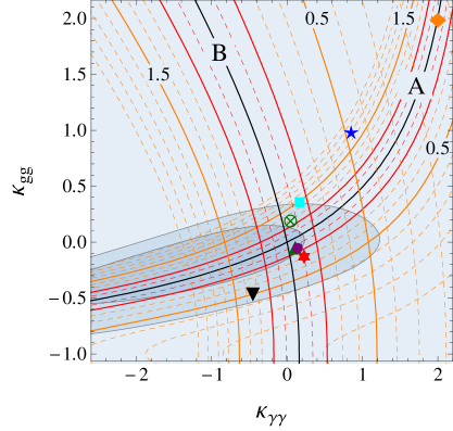
Figure 2: $\kappa^{\prime}_{\gamma\gamma}$ and $\kappa^{\prime}_{gg}$ at the LHC for a Higgs boson with $m_{H}=125$ GeV. The two solid lines correspond to the SM values of the inclusive $\gamma\gamma$ channel (A), and the vector boson fusion production channel (B). On the left panel, the fit using ATLAS data. On the right, the fit using CMS data. Both fits use $\gamma\gamma$, $ZZ$ and $\bar{b}b$ channels. Darker (lighter) blue are the 1, 2 $\sigma$ limits.

IV Conclusion

We have shown how to go beyond the simplest methods when using experimental data to constrain Higgs couplings and account for part of the correlations between measurements. We have presented a parameterisation (Cacciapaglia et al. (2009, 2013)) and we showed how it can be used for testing and putting exclusion limits on models of new physics beyond the Standard Model. In particular our parameterisation is tailored to investigate BSM models, keeping track of the specific correlations among the parameters. It also allows more easily to interpret mass limits and contributions to the loops giving the effective Higgs boson vertices.

We also performed 2 parameter fits of the CMS and ATLAS results using all available channels, showing that they already include all the necessary information and are therefore a good approximation at this stage. More precise measurements of extra channels will require the inclusion of more effective parameters.