Abstract

This paper considers the inverse problem of scattering of time-harmonic acoustic and electromagnetic plane waves by a bounded, inhomogeneous, penetrable obstacle with embedded objects inside. A new method is proposed to prove that the inhomogeneous penetrable obstacle can be uniquely determined from the far-field pattern at a fixed frequency, disregarding its contents. Our method is based on constructing a well-posed interior transmission problem in a small domain associated with the Helmholtz or modified Helmholtz equation and the Maxwell or modified Maxwell equations. A key role is played by the smallness of the domain which ensures that the lowest transmission eigenvalue is large so that a given wave number $k$ is not an eigenvalue of the interior transmission problem. Another ingredient in our proofs is a priori estimates of solutions to the transmission scattering problems with data in $L^{p}$ ($1<p<2$), which are established in this paper by using the integral equation method. A main feature of the new method is that it can deal with the acoustic and electromagnetic cases in a unified way and can be easily applied to deal with inverse scattering by unbounded rough interfaces.

Keywords: Uniqueness, inverse scattering problem, far-field pattern, penetrable obstacle, transmission problem, interior transmission problem, embedded obstacles.

1 Introduction

Consider the problem of scattering of a time-harmonic acoustic or electromagnetic wave by an inhomogeneous penetrable obstacle containing possibly some embedded objects and surrounded by a homogeneous background medium. This problem occurs in various applications such as radar and sonar, remote sensing, geophysics, medical imaging and nondestructive testing.

Denote by $D$ the bounded penetrable obstacle in ${\mathbb{R}}^{3}$ which may contain certain embedded objects denoted by $D_{b}$, that is, $D_{b}\Subset D$. Here, $D$ is assumed to be an open bounded domain in ${\mathbb{R}}^{3}$ with a smooth boundary $\partial D\in C^{2}$ and $D_{b}=\bigcup_{j=1}^{m}D_{b}^{(j)}$ with $D_{b}^{(j_{1})}\cap D_{b}^{(j_{2})}=\emptyset$ if $j_{1}\not=j_{2}$. Denote by $n(x)$ the refractive index characterizing the inhomogeneous medium in ${\mathbb{R}}^{3}\setminus\overline{D_{b}}$ and assume that $n=1$ in ${\mathbb{R}}^{3}\setminus\overline{D}$, $n\in L^{\infty}(D\setminus\overline{D}_{b})$, ${\rm Re}(n)>0$ and ${\rm Im}(n)\geq 0$ in $D\setminus\overline{D}_{b}$. Then the scattering problem of a time-harmonic plane acoustic wave is modeled by the transmission problem

$$\Delta u+k^{2}u=0 \mbox{in}\;\;{\mathbb{R}}^{3}\setminus\overline{D},$$ (1.1)

$$\Delta v+k^{2}nv=0 \mbox{in}\;\;D\setminus\overline{D}_{b},$$ (1.2)

$$u-v=0,\quad\frac{\partial u}{\partial\nu}-\lambda\frac{\partial v}{\partial\nu}=0 \mbox{on}\;\;\partial D,$$ (1.3)

$$\mathscr{B}(v)=0 \mbox{on}\;\;\partial D_{b},$$ (1.4)

$$\lim_{r\rightarrow\infty}r\Big{(}\frac{\partial u^{s}}{\partial r}-iku^{s}\Big{)}=0 r=|x|,$$ (1.5)

where $\lambda>0$ is the transmission coefficient depending on the properties of the media in $D\setminus\overline{D}_{b}$ and ${\mathbb{R}}^{3}\setminus\overline{D}$, $u:=u^{i}+u^{s}$ denotes the total field in ${\mathbb{R}}^{3}\setminus\overline{D}$, $u^{i}=e^{ikx\cdot d}$ is the incident plane wave, $u^{s}$ is the scattered wave, and $\nu$ is the unit normal on $\partial D$ directed into the exterior of $D$. Here, the wave number $k>0$ is given by $k=\omega/c$ with the frequency $\omega>0$ and the sound speed $c>0$ and $d\in{\mathbb{S}}^{2}$ is the incident direction. $\mathscr{B}$ denotes the boundary condition imposed on the boundary $\partial D_{b}$ of the embedded obstacle $D_{b}$ satisfying that $\mathscr{B}(v):=v$ if $D_{b}$ is a sound-soft obstacle, and $\mathscr{B}v:=\partial_{\nu}v$ with the outward normal $\nu$ directing into $D\setminus\overline{D_{b}}$ if $D_{b}$ is a sound-hard obstacle. Further, we have $\mathscr{B}v:=\partial_{\nu}v+\beta v$ on an open subset $\Gamma\subset\partial D_{b}$ (with the impedance coefficient $\beta$ such that ${\rm Im}(\beta)\geq 0$) and $\mathscr{B}v:=v$ on $\partial D_{b}\setminus\overline{\Gamma}$ if $D_{b}$ is a mixed-type obstacle.

In the case $\lambda=1$ the scattering problem (1.1)-(1.5) becomes

$$\Delta u+k^{2}nu=0 \mbox{in}\;\;{\mathbb{R}}^{3}\setminus\overline{D_{b}},$$ (1.6)

$$\mathscr{B}(v)=0 \mbox{on}\;\;\partial D_{b},$$ (1.7)

$$\lim_{r\rightarrow\infty}r\Big{(}\frac{\partial u^{s}}{\partial r}-iku^{s}\Big{)}=0 r=|x|,$$ (1.8)

which is also called the medium scattering problem with embedded objects.

The condition (1.5) (or (1.8)) is referred to the Sommerfeld radiation condition which allows the following asymptotic behavior of the scattered field $u^{s}$:

$$u^{s}(x;d)=\frac{e^{ik|x|}}{4\pi|x|}\left\{u^{\infty}(\widehat{x};d)+O\Big{(}\frac{1}{|x|}\Big{)}\right\},\qquad|x|\rightarrow\infty$$ (1.9)

uniformly in all directions $\widehat{x}=x/|x|\in{\mathbb{S}}^{2}$, where $u^{\infty}$ is defined on the unit sphere ${\mathbb{S}}^{2}$ and known as the far field pattern of the scattered field $u^{s}$.

We also consider the problem of scattering of a time-harmonic electromagnetic plane wave by the inhomogeneous penetrable obstacle $D$ with the embedded obstacle $D_{b}$ and surrounded by a homogeneous background medium. This problem can be formulated as follows:

$${\rm curl\,}E-ikH=0,\quad{\rm curl\,}H+ikE=0 \mbox{in}\;\;{\mathbb{R}}^{3}\setminus\overline{D},$$ (1.10)

$${\rm curl\,}G-ikF=0,\quad{\rm curl\,}F+ikn(x)G=0 \mbox{in}\;\;D\setminus\overline{D_{b}},$$ (1.11)

$$\nu\times E-\nu\times G=0,\quad\nu\times H-\lambda_{H}\nu\times F=0 \mbox{on}\;\;\partial D,$$ (1.12)

$$\mathscr{B}_{E}(G)=0 \mbox{on}\;\;\partial D_{b},$$ (1.13)

$$\lim_{r\rightarrow\infty}r(H^{s}\times\widehat{x}-E^{s})=0 r=|x|,$$ (1.14)

where $E,G$ are the electric fields, $H,F$ are the magnetic fields, $E=E^{i}+E^{s}$ and $H=H^{i}+H^{s}$ in ${\mathbb{R}}^{3}\setminus\overline{D}$ with the incident plane wave

$$E^{i}(x)=\frac{i}{k}{\rm curl\,}{\rm curl\,}pe^{ikx\cdot d},\qquad H^{i}(x)=\frac{1}{ik}{\rm curl\,}E^{i}(x).$$

Here, $\lambda_{H}=\mu_{0}/\mu_{1}$, $k^{2}=\omega^{2}\varepsilon_{0}\mu_{0}$ is the wave number, $n=(\varepsilon_{1}+i\sigma_{1}/\omega)\mu_{1}/(\varepsilon_{0}\mu_{0})$ is the refractive index of the inhomogeneous medium in $D\setminus\overline{D}_{b}$ with electric permittivity $\varepsilon_{1},$ magnetic permeability $\mu_{1}$ and electric conductivity $\sigma_{1}\geq 0$ differing from the electric permittivity $\varepsilon_{0},$ magnetic permeability $\mu_{0}$ and electric conductivity $\sigma_{0}=0$ of the surrounding medium ${\mathbb{R}}^{3}\setminus\overline{D}$, $d$ is the incident direction and $p$ is the polarization vector. Similarly, $\mathscr{B}_{E}$ denotes the boundary condition on $\partial D_{b}$, which corresponds to a perfect conductor condition if $\mathscr{B}_{E}(G):=\nu\times G=0$ and an impedance condition if $\mathscr{B}_{E}(G):=\nu\times{\rm curl\,}G-i\rho_{E}(\nu\times G)\times\nu=0$ with a positive constant $\rho_{E}$. In addition, the condition (1.14) is known as the Silver-Müller radiation condition, which leas to the asymptotic behaviors:

$$E^{s}(x) = \frac{e^{ik|x|}}{|x|}\left\{E^{\infty}(\widehat{x};d;p)+O\Big{(}\frac{1}{|x|}\Big{)}\right\},\qquad|x|\rightarrow\infty$$ (1.15)

$$H^{s}(x) = \frac{e^{ik|x|}}{|x|}\left\{H^{\infty}(\widehat{x};d;p)+O\Big{(}\frac{1}{|x|}\Big{)}\right\},\qquad|x|\rightarrow\infty$$ (1.16)

uniformly for all $\widehat{x}=x/|x|\in{\mathbb{S}}^{2}$, where $E^{\infty}$ and $H^{\infty}(=\widehat{x}\times E^{\infty})$ defined on ${\mathbb{S}}^{2}$ are called the far field patterns of the electric field $E^{s}$ and the magnetic field $H^{s}$, respectively.

In the case $\lambda_{H}=1$ we consider the medium scattering problem without embedded obstacles:

$${\rm curl\,}E-ikH=0,\quad{\rm curl\,}H+ikn(x)E=0 \mbox{in}\;\;{\mathbb{R}}^{3},$$ (1.17)

$$\lim_{r\rightarrow\infty}r(H^{s}\times\widehat{x}-E^{s})=0 r=|x|,$$ (1.18)

where $E=E^{i}+E^{s}$ and $H=H^{i}+H^{s}$ in ${\mathbb{R}}^{3}$, $n=1$ in ${\mathbb{R}}^{3}\setminus\overline{D}$ and $n=(\varepsilon_{1}+i\sigma_{1}/\omega)\mu_{1}/(\varepsilon_{0}\mu_{0})$ in $D$ with $n\in L^{\infty}(D)$.

The existence of a unique solution to the transmission scattering problems (1.1)-(1.5) and (1.10)-(1.14) (or the medium scattering problems (1.6)-(1.8) and (1.17)-(1.18)) can be established by the variational approach or the integral equation method [32, 33, 34, 35, 36]. In this paper, we will assume that the transmission scattering problems (1.1)-(1.5) and (1.10)-(1.14) (or the medium scattering problems (1.6)-(1.8) and (1.17)-(1.18)) are well-posed and study the inverse scattering problem: given $k$, $\lambda$ or $\lambda_{H}$, determine the penetrable obstacle $D$ (or the support $D$ of the inhomogeneous medium in the case $\lambda=1$ or $\lambda_{H}=1$) from a knowledge of $u^{\infty}(\widehat{x};d)$ or $E^{\infty}(\widehat{x};d;p)$ for all $\widehat{x},d\in{\mathbb{S}}^{2}$ and $p\in{\mathbb{R}}^{3}$, disregarding its contents $n$ and $D_{b}$.

In the case $D_{b}=\emptyset$, many uniqueness results have been obtained in determining the penetrable obstacle $D$. The first such uniqueness result was established by Isakov [22] in 1990. The idea is to construct singular solutions of the scattering problem with respect to two different penetrable obstacles with identical far-field patterns, based on the variational method. In 1993, Kirsch and Kress [29] greatly simplified Isakov’s method by considering classical scattering solutions and using the integral equation technique to establish a priori estimates of the solution on some part of the interface $\partial D$. In [29] the method was also extended to the case of Neumann boundary conditions (corresponding to impenetrable, sound-hard obstacles). Since then, the idea has been extensively studied and applied to establish uniqueness results for many other inverse scattering problems with transmission or conductive boundary conditions as well as other boundary conditions (see, e.g., [13, 15, 23, 30, 34, 35, 36, 38, 45, 46] and the references quoted there). The idea of Isakov has also been modified to establish uniqueness results for inverse electromagnetic scattering problems both by a penetrable, inhomogeneous, isotropic obstacle $D$ in [17] under the condition that the boundary $\partial D$ is in $C^{2,\alpha}$ with $0<\alpha<1,$ the refractive index $n\in C^{1,\alpha}(\overline{D})$ is a constant near the boundary $\partial D$ and ${\rm Im}(n(x_{0}))>0$ for some $x_{0}\in D$ and by a penetrable, homogeneous, isotropic obstacle coated with a thin conductive layer in [16]. In [18], Hähner introduced a different technique to prove the unique determination of a penetrable, inhomogeneous, anisotropic obstacle $D$ from a knowledge of the scattered near-fields for all incident plane waves. The method of Hähner is based on a study of the existence, uniqueness and regularity of solutions to the corresponding interior transmission problem in $D$. In [2] Cakoni and Colton extended Hähner’s idea to deal with the case with a penetrable, inhomogeneous, anisotropic obstacle possibly partly coated with a thin layer of a highly conductive material. It seems difficult to apply the idea in [2, 18] to the multi-layered case and the case with embedded obstacles. Further, it was recently proved in [11, 20] that a penetrable, convex polyhedron or polygon obstacle can be uniquely determined by the far-field pattern over all observation directions incited by a single incident plane wave. The arguments used in [11, 20] rely essentially on the expansion of solutions to the Helmholtz equation. Furthermore, it was proved in [39] that a penetrable obstacle with a $C^{2}$-smooth boundary in a two-dimensional domain can be uniquely reconstructed from acoustic measurements made on the boundary of the domain. The method used in [39] uses complex geometrical optics solutions to the Helmholtz equation with polynomial-type phase functions. The result in [39] was extended to the three-dimensional case in [48], to the case with Lipschitz continuous interfaces in [43] and to the isotropic Maxwell system in [24]. These results were further generalized to the elastic wave case with the far-field measurements in [25], based on considering complex geometrical optics solutions to the Lame system with linear or logarithmic phase functions and using $L^{p}$ estimates of the gradients of the solutions to the Lame systems with discontinuous Lame coefficients, and to the anisotropic Maxwell system in [26] by constructing oscillating-decaying-type solutions to the anisotropic Maxwell system.

In the case when there are embedded obstacles in the penetrable obstacle or in an inhomogeneous medium, that is, $D_{b}\not=\emptyset$, it was proved in [32] that the penetrable obstacle $D$ and the embedded obstacle $D_{b}$ can be simultaneously determined from knowledge of the acoustic far-field pattern for incident plane waves under the condition that $n$ is a known constant in $D$. By employing the technique proposed in [17] the uniqueness result was established in [33] for determining the penetrable obstacle $D$ and the embedded obstacle $D_{b}$ simultaneously from knowledge of the electric far-field pattern for incident plane waves provided $n$ is a known complex constant with positive imaginary part in $D$. In [12], Elschner and Hu considered the inverse transmission scattering problem by a two-dimensional, impenetrable obstacle surrounded by an unknown piecewise homogeneous medium and proved that the far-field patterns for all incident and observation directions at a fixed frequency uniquely determine the unknown surrounding medium as well as the impenetrable obstacle. Their method is based on constructing the Green function to a two-dimensional elliptic equation with piecewise constant leading coefficients associated with the direct scattering problem and studying the singularity of the Green function when the point source position approaches the interfaces and the impenetrable obstacle. In [31], the uniqueness result was proved in determining the scattering support of a complex scatterer, possibly consisting of an inhomogeneous medium and impenetrable obstacles, by the acoustic far-field measurements. The technique used in [31] is based essentially on Isakov’s idea in conjunction with the integral equation method and the singular point source with second-order singularity. However, it is difficult to extend the technique of [31] to the case of Maxwell s equations.

It should be pointed out that all the above uniqueness results were obtained under the assumption that the transmission coefficient $\lambda\not=1$ or $\lambda_{H}\not=1$ for the isotropic case or the matrix characterizing the anisotropic medium is different from the identity matrix $I$. In this paper, we propose a new technique to establish uniqueness results for our inverse scattering problem, that is, uniqueness results in determining the penetrable obstacle $D$ (or the support $D$ of the inhomogeneous medium in the case $\lambda=1$ or $\lambda_{H}=1$) from knowledge of the acoustic far-field measurements or the electric far-field measurements at a fixed frequency, disregarding its contents $n$ and $D_{b}$. Our method is based on constructing a well-posed interior transmission problem in a small domain inside $D$ associated with the Helmholtz or Maxwell equations. Here, a key role is played by the smallness of the domain which ensures, for the case $\lambda=1$ or $\lambda_{H}=1$, that the lowest transmission eigenvalue is large so that a given wave number $k$ is not an eigenvalue of the constructed interior transmission problem. This is different from the method used in [2, 18], where the interior transmission problem considered is defined in the whole penetrable obstacle $D$ and may have interior transmission eigenvalues, so the case $\lambda=1$ or $\lambda_{H}=1$ is excluded. Another ingredient in our proofs is a priori estimates of solutions to the transmission scattering problems with data in $L^{p}$ ($1<p<2$) which will be established in this paper by using the integral equation method. These a priori estimates are also expected to be useful on their own right. Our method works for the cases either $\lambda=1$ and $\lambda_{H}=1$ or $\lambda\not=1$ and $\lambda_{H}\not=1$ and can deal with the acoustic and electromagnetic cases in a unified way. Moreover, our method can also deal with the case with unbounded interfaces, as seen in [37]. It should be remarked that reconstruction algorithms, based on the factorization method [28], have been developed in [42, 47] to reconstruct the penetrable obstacle numerically, disregarding its contents.

It is well known that the existence and distribution of the eigenvalues of interior transmission problems play an important role in the linear sampling method [3] and the factorization method [28]. Thus, the existence and computation of the eigenvalues of interior transmission problems have been extensively studied recently (see, e.g. [3, 4, 5, 6, 44] and the references there). In particular, it was proved in [4] that the lowest transmission eigenvalue trends to infinity as the radius of the domain in which the interior transmission problem is defined trends to zero. Thus, for a given wave number $k$ the domain can be taken to be small enough so that $k$ is not an eigenvalue of the interior transmission problem. Our method is motivated by this observation.

The remaining part of the paper is organized as follows. In Sections 2 and 3 we consider the inverse acoustic and electromagnetic scattering problems by penetrable obstacles, respectively. We also utilize the integral equation method to establish a priori estimates of solutions to the acoustic and electromagnetic transmission problems with data in $L^{p}$ ($1<p<2$), which are used in our uniqueness proofs of the inverse scattering problems. It is expected that these a priori estimates are also useful in other applications.

2 The inverse acoustic scattering problem

In this section we introduce the new technique to prove the unique determination of the inhomogeneous penetrable obstacle $D$ (or the support $D$ of the inhomogeneous medium in the case $\lambda=1$) from the far-field pattern $u^{\infty}(\widehat{x};d)$ for all $\widehat{x},d\in S^{2}$, disregarding its contents $n$ and $D_{b}$. Our method is based on constructing a well-posed interior transmission problem in a small domain associated with the Helmholtz or modified Helmholtz equation. Here, a key role is played by the smallness of the domain which ensures that the given wave number $k$ is not a transmission eigenvalue of the constructed interior transmission problem for the case $\lambda=1$. It should be noted that all the previous methods do not work for the case $\lambda=1$. For the case $\lambda\not=1$ which has been considered previously, our method gives a simplified proof. Furthermore, our method also works for the electromagnetic case, as shown in the next section, and for the case of unbounded interfaces (see [37]).

2.1 Interior transmission problems

Let $\Omega\subset{\mathbb{R}}^{3}$ be a simply connected and bounded domain with $\partial\Omega\in C^{2}$. In the case $\lambda\neq 1$ we consider the following modified interior transmission problem (MITP):

$$\triangle U-U=\rho_{1} \text{in}\;\;\Omega,$$ (2.1)

$$\triangle V-V=\rho_{2} \text{in}\;\;\Omega,$$ (2.2)

$$U-V=f_{1},\;\lambda\frac{\partial U}{\partial\nu}-\frac{\partial V}{\partial\nu}=f_{2} \text{on}\;\;\partial\Omega,$$ (2.3)

where $\rho_{0},\rho_{1}\in L^{2}(\Omega)$, $f_{1}\in H^{{1}/{2}}(\partial\Omega)$ and $f_{2}\in H^{-{1}/{2}}(\partial\Omega)$. This problem has been studied in [3], and the following result was obtained (see [3, Theorem 6.7]).

Lemma 2.1.

([3, Theorem 6.7]) If $\lambda\not=1$ then the problem (MITP) has a unique solution $(U,V)\in H^{1}(\Omega)\times H^{1}(\Omega)$ such that

$$\|U\|_{H^{1}(\Omega)}+\|V\|_{H^{1}(\Omega)}\leq C\big{(}\|\rho_{1}\|_{L^{2}(\Omega)}+\|\rho_{2}\|_{L^{2}(\Omega)}+\|f_{1}\|_{H^{{1}/{2}}(\partial\Omega)}+\|f_{2}\|_{H^{-{1}/{2}}(\partial\Omega)}\big{)}.$$

In the case $\lambda=1$ we consider the following interior transmission problem (ITP):

$$\triangle U+k^{2}n(x)U=0 \text{in}\;\;\Omega,$$ (2.4)

$$\triangle V+k^{2}V=0 \text{in}\;\;\Omega,$$ (2.5)

$$U-V=f_{1},\;\;\frac{\partial U}{\partial\nu}-\frac{\partial V}{\partial\nu}=f_{2} \text{on}\;\;\partial\Omega,$$ (2.6)

where $f_{1}\in H^{{1}/{2}}(\partial\Omega)$ and $f_{2}\in H^{-{1}/{2}}(\partial\Omega)$. This problem has been studied in [4].

Let $w:=U-V$. Then it is easy to see that $w$ satisfies the fourth-order equation

$$(\triangle+k^{2}n)\frac{1}{n-1}(\triangle+k^{2})w=0$$ (2.7)

with the boundary conditions $\gamma_{0}w=f_{1}$ and $\gamma_{1}w=f_{2}$. Here, $\gamma_{j}$ $(j=0,1)$ denotes the $j$th-order trace operator.

Define the Hilbert space

$$H^{1}_{\triangle}(\Omega)=\{w\in H^{1}(\Omega):\;\Delta w\in L^{2}(\Omega)\}$$

with the norm $\|w\|^{2}_{H^{1}_{\Delta}(\Omega)}=\|w\|^{2}_{H^{1}(\Omega)}+\|\Delta w\|^{2}_{L^{2}(\Omega)}$. Using the Green’s theorem, we easily prove that $\gamma_{0}w\in H^{{1}/{2}}(\partial\Omega)$, $\gamma_{1}w\in H^{-{1}/{2}}(\partial\Omega)$. In particular, if $\gamma_{0}w=\gamma_{1}w=0$ for all $w\in H^{1}_{\Delta}(\Omega)$, then $H^{1}_{\Delta}(\Omega)=H^{2}_{0}(\Omega)$.

We assume that the data $f_{1}\in H^{{1}/{2}}(\partial\Omega)$ and $f_{2}\in H^{-{1}/{2}}(\partial\Omega)$ satisfy the condition (C) with some $w_{0}\in H^{1}_{\Delta}(\Omega),$ that is, there exists a function $w_{0}\in H^{1}_{\Delta}(\Omega)$ such that $\gamma_{0}w_{0}=f_{1}$, $\gamma_{1}w_{0}=f_{2}.$ Then the interior transmission problem (ITP) is equivalent to the variational problem: Find $w\in H^{1}_{\Delta}(\Omega)$ with $\gamma_{0}w=f_{1}$ and $\gamma_{1}w=f_{2}$ such that

$$a(w,h):=\int_{\Omega}\frac{1}{n-1}(\triangle+k^{2})w(\Delta+k^{2}n)\overline{h}dx=0\quad\text{for\;all\;}\;h\in H^{2}_{0}(\Omega).$$ (2.8)

Let $\widetilde{w}:=w-w_{0}\in H^{2}_{0}(\Omega)$. Then the variational problem (2.8) is equivalent to the problem: Find $\widetilde{w}\in H^{2}_{0}(\Omega)$ such that

$$a(\widetilde{w},h)=-a(w_{0},h)\quad\text{for\;all\;}\;h\in H^{2}_{0}(\Omega).$$ (2.9)

Based on (2.9), the following result can be established (see [4] for a proof).

Lemma 2.2.

([4, Lemma 2.4]) If $n(x)>1+r_{0}$ or $0<n(x)<1-r_{1}$ with some constants $r_{0},r_{1}>0$, then

$$a(\widetilde{w},\widetilde{w})\geq C\|\widetilde{w}\|^{2}_{H^{2}_{0}(\Omega)},\quad\forall\widetilde{w}\in H^{2}_{0}(\Omega)$$

for $0<k^{2}<\min\{\lambda_{1}(\Omega),\lambda_{1}(\Omega)/\sup(n)\},$ where $\lambda_{1}(\Omega)$ is the first Dirichlet eigenvalue of the operator $-\triangle$ in $\Omega$.

By Lemma 2.2 the following result can be easily obtained.

Corollary 2.3.

Assume that $f_{1},f_{2}$ satisfy the condition (C) with $w_{0}\in H^{1}_{\Delta}(\Omega).$ For any fixed $k>0$, if the diameter of $\Omega$ is small enough (so $\lambda_{1}(\Omega)$ is large enough) so that $k^{2}<\min\{\lambda_{1}(\Omega),\lambda_{1}(\Omega)/\sup(n)\}$, then the interior transmission problem (ITP) has a unique solution $(U,V)\in L^{2}(\Omega)\times L^{2}(\Omega)$ with

$$\|U\|_{L^{2}(\Omega)}+\|V\|_{L^{2}(\Omega)}\leq C\|w_{0}\|_{H^{1}_{\Delta}(\Omega)}.$$ (2.10)

Proof.

For any fixed $k>0$, if the diameter of $\Omega$ is small enough so that $k^{2}<\min\{\lambda_{1}(\Omega),\lambda_{1}(\Omega)/\sup(n)\}$, then, by Lemma 2.2 it follows that

$$a(\widetilde{w},\widetilde{w})\geq C\|\widetilde{w}\|^{2}_{H^{2}_{0}(\Omega)}\quad\mbox{for all}\;\;\widetilde{w}\in H^{2}_{0}(\Omega).$$

This, together with the Lax-Milgram theorem, implies that the variational problem (2.9) has a unique solution $\widetilde{w}\in H^{2}_{0}(\Omega)$ satisfying the estimate

$$\|\widetilde{w}\|_{H^{2}_{0}(\Omega)}\leq C\|w_{0}\|_{H^{1}_{\Delta}(\Omega)}.$$ (2.11)

Define $U:=[{1}/({n-1})](\Delta+k^{2})w$, $V:=U-w$. Then it is easy to see that $(U,V)\in L^{2}(\Omega)\times L^{2}(\Omega)$, with $U-V\in H^{2}_{0}(\Omega)$, is the unique solution to the interior transmission problem (ITP). The estimate (2.10) follows easily from (2.11) and the fact that $w=\widetilde{w}+w_{0}$. ∎

Remark 2.4.

The uniqueness result for the case $\lambda\not=1$ corresponds to the well-posed problem (MITP), whilst that for the case $\lambda=1$ corresponds to the much harder problem (ITP) which is not necessarily well-posed for all wavenumbers $k$ if $\Omega$ is not small, as shown in Lemma 2.1 and Corollary 2.3. This explains clearly why the transmission coefficient $\lambda$ is assumed not to be $1$ (i.e., $\lambda\not=1$) in all the previous methods of the uniqueness proofs of the inverse problems.

2.2 A priori estimates for the transmission problems with $L^{p}$ boundary data

In this subsection, we establish a priori estimates of solutions to the acoustic transmission problem with boundary data in $L^{p}$ ($1<p\leq 2$), employing the integral equation method. These a priori estimates are needed later in the uniqueness proof of the inverse problem and are also interesting on their own right.

Consider the general acoustic transmission problem

$$\triangle w_{1}+k^{2}w_{1}=0 \text{in}\;\;{\mathbb{R}}^{3}\setminus\overline{D},$$ (2.12)

$$\triangle w_{2}+k^{2}n(x)w_{2}=0 \text{in}\;\;D\setminus\overline{D_{b}},$$ (2.13)

$$w_{1}-\gamma w_{2}=f_{1},\;\;\frac{\partial w_{1}}{\partial\nu}-\frac{\partial w_{2}}{\partial\nu}=f_{2} \text{on}\;\;\partial D,$$ (2.14)

$$\mathscr{B}(w_{2})=0 \text{on}\;\;\partial D_{b},$$ (2.15)

$$\frac{\partial w_{1}}{\partial r}-ikw_{1}=o\Big{(}\frac{1}{r}\Big{)} r=|x|\rightarrow\infty,$$ (2.16)

where $f_{1},f_{2}\in L^{p}(\partial D)$ with $1<p<2$ and $\gamma=1/\lambda$.

We introduce the single- and double-layer boundary operators

$$(S_{\rm{e}\rm{e}}\phi)(x) := \int_{\partial D}\Phi(x,y)\phi(y)ds(y),\quad x\in\partial D,$$

$$(K_{\rm{e}\rm{e}}\phi)(x) := \int_{\partial D}\frac{\partial\Phi(x,y)}{\partial\nu(y)}\phi(y)ds(y),\quad x\in\partial D$$

and the their normal derivative operators

$$(K^{\prime}_{\rm{e}\rm{e}}\phi)(x) := \int_{\partial D}\frac{\partial\Phi(x,y)}{\partial\nu(x)}\phi(y)ds(y),\quad x\in\partial D,$$

$$(T_{\rm{e}\rm{e}}\phi)(x) := \frac{\partial}{\partial\nu(x)}\int_{\partial D}\frac{\partial\Phi(x,y)}{\partial\nu(y)}\phi(y)ds(y),\quad x\in\partial D.$$

Similarly, we also introduce the boundary operators $S_{\rm{i}\rm{i}}$, $K_{\rm{i}\rm{i}}$, $K^{\prime}_{\rm{i}\rm{i}}$ and $T_{\rm{i}\rm{i}}$ defined on $\partial D_{b}$ as well as $S_{\rm{t}\rm{h}}$, $K_{\rm{t}\rm{h}}$, $K^{\prime}_{\rm{t}\rm{h}}$ and $T_{\rm{t}\rm{h}}$ with $\rm{t,h}=\rm{e,i}$, respectively, where, for example, $S_{\rm{e}\rm{i}}$ is defined similarly as $S_{\rm{e}\rm{e}}$ but with $x\in\partial D_{b}$. It follows from [40, Lemma 9] and [41, Lemma 1] that the operators $S_{\rm{p}\rm{p}},K_{\rm{p}\rm{p}}$ and $K^{\prime}_{\rm{p}\rm{p}}$ with $\rm{p}=\rm{e,i}$ are both bounded and compact in $L^{q}(\partial D)$ ($1<q<\infty$).

Theorem 2.5.

For $f_{1},f_{2}\in L^{p}(\partial D)$ with $4/3\leq p\leq 2$ the transmission problem $(\ref{2.11})-(\ref{2.14})$ has a unique solution $(w_{1},w_{2})\in L^{2}_{\rm{loc}}({\mathbb{R}}^{3}\setminus\overline{D})\times L^{2}(D_{b})$ satisfying that

$$\|w_{1}\|_{L^{2}_{\rm{loc}}({\mathbb{R}}^{3}\setminus\overline{D})}+\|w_{2}\|_{L^{2}(D\setminus\overline{D_{b}})}\leq C(\|f_{1}\|_{L^{p}(\partial D)}+\|f_{2}\|_{L^{p}(\partial D)}).$$ (2.17)

Proof.

We only consider the case with an impedance condition on $\partial D_{b}$, that is, $\mathscr{B}(w_{2})=\partial w_{2}/\partial\nu+i\rho w_{2}=0$. The other case can be treated similarly.

Step 1. Assume that $k^{2}n(x)\equiv k_{1}^{2}>0$ is a constant. We seek a solution of the problem (2.12)-(2.16) in the form

$$w_{1}(x) = \int_{\partial D}\Phi(x,y)\phi(y)ds(y)+\int_{\partial D}\frac{\partial\Phi(x,y)}{\partial\nu(y)}\psi(y)ds(y),\quad x\in{\mathbb{R}}^{3}\setminus\overline{D}$$ (2.18)

$$w_{2}(x) = \int_{\partial D}\Phi_{1}(x,y)\phi(y)ds(y)+\int_{\partial D}\frac{\partial\Phi_{1}(x,y)}{\partial\nu(y)}\psi(y)ds(y)$$ (2.19)

$$+\int_{\partial D_{b}}\Phi_{1}(x,y)\eta(y)ds(y),\qquad x\in D\setminus\overline{D_{b}},$$

where $\Phi(x,y)=\exp({ik|x-y|})/({4\pi|x-y|})$ and $\Phi_{1}(x,y)=\exp({ik_{1}|x-y|})/({4\pi|x-y|})$.

Then, by the jump relations of the layer potentials (see [41] for the case in $L^{p}$ and [7, 8] for the case in spaces of continuous functions), the transmission problem (2.12)-(2.16) can be reduced to the system of integral equations

$$\left(\begin{array}[]{c}\psi\\ \phi\\ \eta\\ \end{array}\right)+L\left(\begin{array}[]{c}\psi\\ \phi\\ \eta\\ \end{array}\right)=\left(\begin{array}[]{c}hf_{1}\\ -f_{2}\\ 0\\ \end{array}\right)\qquad\text{in}\;\;L^{p}(\partial D)\times L^{p}(\partial D)\times C(\partial D_{b}),$$ (2.29)

where $h:=2/(1+\gamma)$ and the operator $L$ is given by

$$L:=\left(\begin{array}[]{ccc}h(K_{\rm{e}\rm{e}}-\gamma K^{(1)}_{\rm{e}\rm{e}})&h(S_{\rm{e}\rm{e}}-\gamma S^{(1)}_{\rm{e}\rm{e}})&-h\gamma S^{(1)}_{\rm{i}\rm{e}}\\ T^{(1)}_{\rm{e}\rm{e}}-T_{\rm{e}\rm{e}}&K^{\prime(1)}_{\rm{e}\rm{e}}-K^{\prime}_{\rm{e}\rm{e}}&K^{\prime(1)}_{\rm{i}\rm{e}}\\ -2(T^{(1)}_{\rm{e}\rm{i}}+i\rho K^{(1)}_{\rm{e}\rm{i}})&-2(K^{\prime(1)}_{\rm{e}\rm{i}}+i\rho S^{(1)}_{\rm{e}\rm{i}})&-2(K^{\prime(1)}_{\rm{i}\rm{i}}+i\rho S^{(1)}_{\rm{i}\rm{i}})\end{array}\right).$$

Here, the operators $S^{(1)}_{\rm{t}\rm{h}},K^{(1)}_{\rm{t}\rm{h}},K^{\prime(1)}_{\rm{t}\rm{h}}$ and $T^{(1)}_{\rm{t}\rm{h}}$ with $\rm{t,h}=\rm{e,i}$, respectively, are defined similarly as $S_{\rm{t}\rm{h}},K_{\rm{t}\rm{h}},K^{\prime}_{\rm{t}\rm{h}}$ and $T_{\rm{t}\rm{h}}$ with the kernel $\Phi(x,y)$ replaced by $\Phi_{1}(x,y)$. It is easy to see that (2.29) is of Fredholm type since the elements of $L$ are all compact operators in the corresponding Banach spaces. This, together with the uniqueness of the scattering problem (1.1)-(1.5), implies that (2.29) has a unique solution $(\psi,\phi,\eta)^{T}\in L^{p}(\partial D)\times L^{p}(\partial D)\times C(\partial D_{b})$ satisfying the estimate

$$\|\psi\|_{L^{p}(\partial D)}+\|\phi\|_{L^{p}(\partial D)}+\|\eta\|_{L^{\infty}(\partial D_{b})}\leq C(\|f_{1}\|_{L^{p}(\partial D)}+\|f_{2}\|_{L^{p}(\partial D)}).$$ (2.31)

Therefore, we obtain that

$$\left\|\int_{\partial D}\Phi_{1}(\cdot,y)\phi(y)ds(y)\right\|_{L^{2}(D)}=\sup_{g\in L^{2},\|g\|_{L^{2}(D)}=1}\left|\int_{D}\left\{\int_{\partial D}\Phi_{1}(x,y)\phi(y)ds(y)\right\}g(x)dx\right|$$

$$\qquad\qquad=\sup_{g\in L^{2},\|g\|_{L^{2}(D)}=1}\left|\int_{\partial D}\left\{\int_{D}\Phi_{1}(x,y)g(x)dx\right\}\phi(y)ds(y)\right|$$

$$\qquad\qquad\leq|\partial D|^{{1}/{q}}\sup_{g\in L^{2},\|g\|_{L^{2}(D)}=1}\sup_{y\in\partial D}\|\Phi_{1}(\cdot,y)\|_{L^{2}(D)}\|g\|_{L^{2}(D)}\|\phi\|_{L^{p}(\partial D)}$$

$$\qquad\qquad=|\partial D|^{{1}/{q}}\sup_{y\in\partial D}\|\Phi_{1}(\cdot,y)\|_{L^{2}(D)}\|\phi\|_{L^{p}(\partial D)}$$ (2.32)

and

$$\left\|\int_{\partial D}\frac{\partial\Phi_{1}(\cdot,y)}{\partial\nu(y)}\psi(y)ds(y)\right\|_{L^{2}(D)}=\sup_{g\in L^{2},\|g\|_{L^{2}(D)}=1}\left|\int_{D}\left\{\int_{\partial D}\frac{\partial\Phi_{1}(x,y)}{\partial\nu(y)}\psi(y)ds(y)\right\}g(x)dx\right|$$

$$\qquad\qquad=\sup_{g\in L^{2},\|g\|_{L^{2}(D)}=1}\left|\int_{\partial D}\left\{\frac{\partial}{\partial\nu(y)}\int_{D}\Phi_{1}(x,y)g(x)dx\right\}\psi(y)ds(y)\right|$$

$$\qquad\qquad\leq\sup_{g\in L^{2},\|g\|_{L^{2}(D)}=1}\left\|\frac{\partial}{\partial\nu(y)}\int_{D}\Phi_{1}(x,\cdot)g(x)dx\right\|_{L^{q}(\partial D)}\cdot\left\|\psi\right\|_{L^{p}(\partial D)}$$

$$\qquad\qquad\leq\sup_{g\in L^{2},\|g\|_{L^{2}(D)}=1}C\|g\|_{L^{2}(D)}\cdot\left\|\psi\right\|_{L^{p}(\partial D)}=C\left\|\psi\right\|_{L^{p}(\partial D)}$$ (2.33)

with $1/p+1/q=1$. Here, we have used the fact that the volume potential operator is bounded from $L^{2}(D)$ into $W^{2,2}(D)$ (see [14, Theorem 9.9]), and the boundary trace operator is bounded from $W^{1,2}(D)$ into $L^{q}(\partial D)$ for $2\leq q\leq 4$ (see [1, Theorem 5.36]). Further, we derive from [7] that

$$\left\|\int_{\partial D_{b}}\Phi_{1}(\cdot,y)\eta(y)ds\right\|_{L^{\infty}({\mathbb{R}}^{3})} \leq C\|\eta\|_{L^{\infty}(\partial D_{b})}.$$ (2.34)

Then the desired estimate (2.17) follows from (2.18)-(2.19) and (2.31)-(2.34) in the case when $k^{2}n(x)\equiv k^{2}_{1}$.

Step 2. For the general case $n\in L^{\infty}(D\setminus\overline{D}_{b})$, we consider the following problem

$$\triangle W_{1}+k^{2}W_{1}=0 \text{in}\;\;{\mathbb{R}}^{3}\setminus\overline{D},$$ (2.35)

$$\triangle W_{2}+k^{2}n(x)W_{2}=g \text{in}\;\;D\setminus\overline{D_{b}},$$ (2.36)

$$W_{1}-\gamma W_{2}=0,\;\;\frac{\partial W_{1}}{\partial\nu}-\frac{\partial W_{2}}{\partial\nu}=0 \text{on}\;\;\partial D,$$ (2.37)

$$\mathscr{B}(W_{2})=0 \text{on}\;\;\partial D_{b},$$ (2.38)

$$\frac{\partial W_{1}}{\partial r}-ikW_{1}=o\Big{(}\frac{1}{r}\Big{)} r=|x|\rightarrow\infty,$$ (2.39)

where $g:=(k_{1}^{2}-k^{2}n(x))\widetilde{w}_{2}\in L^{2}(D\setminus\overline{D}_{b})$ and $(\widetilde{w}_{1},\widetilde{w}_{2})$ denotes the solution of the problem (2.12)-(2.16) with $k^{2}n(x)\equiv k^{2}_{1}$. By Step 1, we have

$$\|\widetilde{w}_{1}\|_{L^{2}_{\rm{loc}}({\mathbb{R}}^{3}\setminus\overline{D})}+\|\widetilde{w}_{2}\|_{L^{2}(D\setminus\overline{D_{b}})}\leq C(\|f_{1}\|_{L^{p}(\partial D)}+\|f_{2}\|_{L^{p}(\partial D)}).$$ (2.40)

By using the variational method, it can be easily proved that for every $g\in L^{2}(D\setminus\overline{D_{b}})$ the problem (2.35)-(2.39) has a unique solution $(W_{1},W_{2})\in H^{1}_{\rm{loc}}({\mathbb{R}}^{3}\setminus\overline{D})\times H^{1}(D\setminus\overline{D_{b}})$ satisfying the estimate

$$\|W_{1}\|_{H^{1}_{\rm{loc}}({\mathbb{R}}^{3}\setminus\overline{D})}+\|W_{2}\|_{H^{1}(D\setminus\overline{D_{b}})}\leq C\|g\|_{L^{2}(D\setminus\overline{D_{b}})}.$$ (2.41)

Define $w_{1}:=W_{1}+\widetilde{w}_{1}$ and $w_{2}:=W_{2}+\widetilde{w}_{2}$. Then from (2.40) and (2.41) it follows that $(w_{1},w_{2})\in L^{2}_{\rm{loc}}({\mathbb{R}}^{3}\setminus\overline{D})\times L^{2}(D\setminus\overline{D_{b}})$ is the unique solution of the problem (2.12)-(2.16) satisfying the estimate (2.17). The proof is thus complete. ∎

Corollary 2.6.

For $z^{*}\in\partial D$ and for a sufficiently small $\delta>0$ define $z_{j}:=z^{*}+({\delta}/{j})\nu(z^{*})\in{\mathbb{R}}^{3}\setminus\overline{D}$, $j\in{\mathbb{N}}$. Let $(u_{j},v_{j})$ be the solution of the transmission problem $(\ref{1.1})-(\ref{1.4})$ corresponding to the incident point source $u^{i}_{j}=\Phi(x,z_{j})$, $j\in{\mathbb{N}}$. Then

$$\|v_{j}\|_{L^{2}(D\setminus\overline{D_{b}})}\leq C$$ (2.42)

uniformly for $j\in{\mathbb{N}}$.

Proof.

Let $w_{1j}:=u_{j}^{s}-\Phi(x,y_{j})$ and $w_{2j}:=\lambda v_{j}$ with $y_{j}:=z^{*}-({\delta}/{j})\nu(z^{*})\in D\setminus\overline{D_{b}}$. Then $(w_{1},w_{2})$ satisfies the problem (2.12)-(2.16) with

$$f_{1}=f_{1j} := -\Phi(z,z_{j})-\Phi(x,y_{j}),$$

$$f_{2}=f_{2j} := -\frac{\partial\Phi(z,z_{j})}{\partial\nu(z)}-\frac{\partial\Phi(z,y_{j})}{\partial\nu(z)}.$$

Obviously, $f_{1j}\in L^{p}(\partial D)$ is uniformly bounded for $j\in{\mathbb{N}}$, where $1<p<2$. Further, from [9, Lemma 4.2] it is seen that $f_{2j}\in C(\partial D)$ is uniformly bounded for $j\in{\mathbb{N}}$, so $f_{2j}\in L^{p}(\partial D)$ is uniformly bounded for $j\in{\mathbb{N}}$, where $1<p<2$. The estimate (2.42) then follows from Theorem 2.5. ∎

Theorem 2.7.

Let $(u,v)$ be the solution of the scattering problem $(\ref{1.1+})-(\ref{1.4+})$ corresponding to the supper singular point source $u^{i}=\nabla_{x}\Phi(x,z)\cdot\vec{a}$, where $z\in{\mathbb{R}}^{3}\setminus\overline{D}$ and $\vec{a}\in{\mathbb{R}}^{3}$ is a fixed vector. Then $v\in L^{p}(D\setminus\overline{D_{b}})$ and $v-u^{i}\in H^{1}(D\setminus\overline{D_{b}})$ such that

$$\|v\|_{L^{p}(D\setminus\overline{D_{b}})}+\|v-u^{i}\|_{H^{1}(D\setminus\overline{D_{b}})}\leq C(\|u^{i}\|_{L^{p}(D\setminus\overline{D_{b}})}+\|u^{i}\|_{L^{\infty}(\partial D_{b})})$$ (2.43)

for every $p$ with $6/5\leq p<2$.

To prove the estimate (2.43), we reformulate the scattering problem (1.6)-(1.8) as an equivalent Lippmann-Schwinger-type equation. To this end, we introduce the exterior boundary value problem associated with $D_{b}$ and the boundary condition $\mathscr{B}$:

$$\left\{\begin{array}[]{ll}\triangle w+k^{2}w=0&\text{in}\;\;{\mathbb{R}}^{3}\setminus\overline{D_{b}},\\ \mathscr{B}(w)=f&\text{on}\;\;\partial D_{b},\\ \displaystyle\frac{\partial w}{\partial|x|}-ikw=o\left(\frac{1}{|x|}\right)&\text{for}\;\;|x|\to\infty.\end{array}\right.$$ (2.47)

It is well known that the problem (2.47) is well-posed for every $f$ belonging to a suitable Holder or Sobolev space.

Let $G^{s}(\cdot,y)$ be the solution to the problem (2.47) with $f=-\mathscr{B}(\Phi(\cdot,y))$ and let $U(\cdot;y)$ be the solution to the problem (2.47) with $f=-\mathscr{B}(\nabla\Phi(\cdot,y)\cdot\vec{a})$ with $y\in{\mathbb{R}}^{3}\setminus\overline{D_{b}}$. Define

$$G(x,y):=\Phi(x,y)+G^{s}(x,y)\qquad\qquad\text{in}\;\;{\mathbb{R}}^{3}\setminus\overline{D_{b}},$$

$$U^{i}(x;y):=\nabla_{x}\Phi(x,y)\cdot\vec{a}+U(x;y)\qquad\text{in}\;\;{\mathbb{R}}^{3}\setminus\overline{D_{b}}.$$

Then $G(x,y)$ satisfies the problem (2.47) with $f=0$, that is, $G(x,y)$ is the Green function of the problem (2.47) with $f=0$. By the representation theorem for $v(\cdot;z)$, we have

$$v(x;z) = \left(\int_{\partial D}-\int_{\partial D_{b}}\right)\left\{G(x,y)\frac{\partial v(y;z)}{\partial\nu(y)}-\frac{\partial G(x,y)}{\partial\nu(y)}v(y;z)\right\}ds(y)$$ (2.48)

$$-\int_{D\setminus\overline{D_{b}}}k^{2}[1-n(y)]G(x,y)v(y;z)dy,\qquad\qquad\text{for}\;\;x\in D\setminus\overline{D_{b}}.$$

The integral on $\partial D_{b}$ obviously equals to zero due to the boundary condition. Further, the radiation condition for $G(\cdot,x)$ and $v^{s}(\cdot;z)$ yields

$$\int_{\partial D}\left\{G(x,y)\frac{\partial[v(y;z)-U^{i}(y;z)]}{\partial\nu(y)}-\frac{\partial G(x,y)}{\partial\nu(y)}[v(y;z)-U^{i}(y;z)]\right\}ds(y)=0.$$

This, combined with (2.48) and the Green theorem, implies that the solution $v$ of the scattering problem (1.6)-(1.8) with $u^{i}=\nabla_{x}\Phi(x,z)\cdot\vec{a}$ satisfies the Lippmann-Schwinger-type equation

$$v(x;z)=U^{i}(x;z)-k^{2}\int_{D\setminus\overline{D_{b}}}[1-n(y)]G(x,y)v(y;z)dy.$$ (2.49)

Conversely, it is easy to prove that the solution of (2.49) also satisfies the scattering problem (1.6)-(1.8).

Remark 2.8.

The equivalence between the scattering problem (1.6)-(1.8) and the Lippmann-Schwinger-type equation (2.49) still holds for a general incident field $u^{i}$ such as a plane wave $u^{i}=e^{ikx\cdot d}$ with $d\in S^{2}$ and a point source $u^{i}=\Phi(x,y)$ with $y\in{\mathbb{R}}^{3}\setminus\overline{D}$.

Proof of Theorem 2.7. Define the volume operator $T$ in $L^{p}(D\setminus\overline{D_{b}})$ by

$$(T\varphi)(x):=k^{2}\int_{D\setminus\overline{D_{b}}}[1-n(y)]G(x,y)\varphi(y)dy\quad\text{in}\;D\setminus\overline{D_{b}}.$$

Then we have

$$(I+T)v(\cdot;z)=U^{i}(\cdot;z)\quad\text{in}\;\;L^{p}(D\setminus\overline{D_{b}})$$ (2.50)

since $U^{i}(\cdot;z)\in L^{p}(D\setminus\overline{D_{b}})$ for $6/5\leq p<2$. It follows from [14, Theorem 9.9] that $T$ is bounded from $L^{p}(D\setminus\overline{D_{b}})$ into $W^{2,p}(D\setminus\overline{D_{b}})$ and therefore compact in $L^{p}(D\setminus\overline{D_{b}})$. Thus, and by the uniqueness result for the scattering problem (1.6)-(1.8), the operator $I+T$ is of Fredholm type with index zero. The Fredholm alternative then implies the existence of a unique solution $v$ in $L^{p}(D\setminus\overline{D_{b}})$ to (2.50) with the estimate

$$\|v(\cdot;z)\|_{L^{p}(D\setminus\overline{D_{b}})}\leq C\|U^{i}(\cdot;z)\|_{L^{p}(D\setminus\overline{D_{b}})}\leq C(\|u^{i}(\cdot;z)\|_{L^{p}(D\setminus\overline{D_{b}})}+\|u^{i}(\cdot;z)\|_{L^{\infty}(\partial D_{b})})$$ (2.51)

for $6/5\leq p<2$. From this, the well-posedness of (2.47) and the embedding result that $W^{2,p}(D\setminus\overline{D_{b}})\hookrightarrow H^{1}(D\setminus\overline{D_{b}})$ for $6/5\leq p<2$, the required estimate (2.43) follows. The proof is thus complete. $\Box$

2.3 Uniqueness of the inverse problem

Based on Lemma 2.1, Corollary 2.3 and Theorems 2.5 and 2.7, we shall prove the global uniqueness result in determining the inhomogeneous penetrable obstacle $D$ disregarding its contents if the transmission coefficient $\lambda\not=1$ or if the refractive index $n$ has a singularity at the interface $\partial D$ in the case $\lambda=1$, that is, $n$ satisfies the following assumption (A).

Assumption (A): there exists an open neighborhood of $\partial D$, $\mathcal{O}(\partial D)\Subset D\setminus\overline{D_{b}}$, and a positive constant $\varepsilon_{0}>0$ such that $|n(x)-1|\geq\varepsilon_{0}$ for a.e. $x\in\mathcal{O}(\partial D)$.

Theorem 2.9.

Given $k>0$, let $u^{\infty}(\widehat{x};d)$ and $\widetilde{u}^{\infty}(\widehat{x};d)$ be the far-field patterns of the scattering solutions to the transmission problem $(\ref{1.1})-(\ref{1.4})$ (or the scattering problem $(\ref{1.1+})-(\ref{1.4+})$) with respect to the penetrable obstacle $D$ with the refractive index $n\in L^{\infty}(D\setminus\overline{D_{b}})$ as well as the embedded obstacle $D_{b}$ and the penetrable obstacle $\widetilde{D}$ with the refractive index $\widetilde{n}\in L^{\infty}(\widetilde{D}\setminus\overline{\widetilde{D}_{b}})$ as well as the embedded obstacle $\widetilde{D}_{b}$, respectively. Assume that $u^{\infty}(\widehat{x};d)=\widetilde{u}^{\infty}(\widehat{x};d)$ for all $\widehat{x},d\in{\mathbb{S}}^{2}$.

(i) If $\lambda\not=1$, then $D=\widetilde{D}$.

(ii) If $\lambda=1$ and $n,\widetilde{n}$ satisfy Assumption (A), then $D=\widetilde{D}$.

Proof.

Assume that $D\neq\widetilde{D}$. Without loss of generality, choose $z^{*}\in\partial D\setminus\partial\widetilde{D}$ and define

$$z_{j}:=z^{*}+({\delta}/{j})\nu(z^{*}),\;\;j=1,2,\ldots$$

with a sufficiently small $\delta>0$ such that $z_{j}\in B$, where $B$ denotes a small ball centered at $z^{*}$ such that $B\cap(\overline{\widetilde{D}\cup D_{b}})=\emptyset$. See Figure 1.

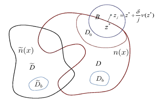
Figure 1: Two different scattering obstacles

(i) Let $\lambda\neq 1$ and let $(u_{j},v_{j})$, $(\widetilde{u_{j}},\widetilde{v_{j}})$ be the unique solution to the transmission problem (1.1)-(1.5) with respect to $D$ with refractive index $n$ and the embedded obstacle $D_{b}$, $\widetilde{D}$ with refractive index $\widetilde{n}$ and the embedded obstacle $\widetilde{D}_{b}$, respectively, corresponding to the incident point source

$$u^{i}_{j}(x):=\Phi(x,z_{j})=\frac{\exp({ik|x-z_{j}|})}{4\pi|x-z_{j}|},\qquad j=1,2,\ldots.$$

The assumption that $u^{\infty}(\widehat{x};d)=\widetilde{u}^{\infty}(\widehat{x};d)$ for all $\widehat{x},d\in{\mathbb{S}}^{2}$, together with Rellich’s lemma and the denseness result [7, Theorems 5.4 and 5.5], implies that

$$u^{s}_{j}(x)=\widetilde{u}^{s}_{j}(x)\qquad\mbox{in}\;\;\overline{G},\qquad j=1,2,\ldots,$$ (2.52)

where $G$ denotes the unbounded component of ${\mathbb{R}}^{3}\setminus\overline{(D\cup\widetilde{D})}$.

Since $z^{*}\in\partial D\setminus\partial\widetilde{D}$ and $\partial D\in C^{2}$, there is a small smooth ($C^{2}$) domain $D_{0}$ such that $B\cap D\subset D_{0}\subset D\setminus\overline{(\widetilde{D}\cup D_{b})}$. Define $U_{j}:=v_{j}$, $V_{j}:=\widetilde{u}_{j}$ in $D_{0}$. Then $(U_{j},V_{j})$ satisfies the modified interior transmission problem (MITP) with $\Omega=D_{0}$ and

$$\rho_{1}(j):=-(k^{2}n+1)v_{j}|_{D_{0}},\quad\quad\rho_{2}(j):=-(k^{2}+1)\widetilde{u}_{j}|_{D_{0}},$$

$$f_{1}(j):=(v_{j}-\widetilde{u}_{j})|_{\partial D_{0}},\quad\quad\quad f_{2}(j):=(\lambda\partial v_{j}/\partial\nu-\partial\widetilde{u}_{j}/\partial\nu)|_{\partial D_{0}}.$$

From (2.52) it is clear that $f_{1}(j)=f_{2}(j)=0$ on $\Gamma_{1}:=\partial D_{0}\cap\partial D$. Since $z^{*}$ has a positive distance from $\widetilde{D}$, the well-posedness of the transmission problem (1.1)-(1.5) implies that

$$\|\widetilde{u}_{j}^{s}\|_{H^{2}(D_{0})}\leq C\quad\mbox{uniformly\;for}\;\;j\in{\mathbb{N}}.$$ (2.53)

This implies that $\rho_{2}(j)\in L^{2}(D_{0})$ is uniformly bounded for $j\in{\mathbb{N}}$ since $\Phi(\cdot,z_{j})\in L^{2}(D_{0})$ is uniformly bounded for $j\in{\mathbb{N}}$. From Corollary 2.6 it is known that $\rho_{1}(j)$ is uniformly bounded in $L^{2}(D_{0})$ for $j\in{\mathbb{N}}$.

We now prove that $f_{1}(j)$ and $f_{2}(j)$ are uniformly bounded in $H^{{1}/{2}}(\partial D_{0})$ and $H^{-{1}/{2}}(\partial D_{0})$, respectively, for $j\in{\mathbb{N}}$. To this end, define $w_{j}:=v_{j}-\widetilde{u}_{j}^{s}-\Phi(\cdot,z_{j})=v_{j}-\widetilde{u}_{j}$. Then $w_{j}\in H^{2}(D\setminus\overline{(\widetilde{D}\cup D_{b})})$ for every $j\in{\mathbb{N}}$ since $z_{j}\in{\mathbb{R}}^{3}\setminus\overline{D}$ and is a solution to the problem

$$\triangle w_{j}=g_{j}\quad\text{in}\;\;D\setminus\overline{(\widetilde{D}\cup D_{b})},\quad\quad w_{j}|_{\Gamma_{1}}=0,$$

where $g_{j}:=k^{2}[\Phi(\cdot,z_{j})+\widetilde{u}_{j}^{s}-nv_{j}]\in L^{2}(D\setminus\overline{(\widetilde{D}\cup D_{b})})$. It follows from [14, Theorem 9.13] that

$$\|w_{j}\|_{H^{2}(D_{0})}\leq C\big{(}\|w_{j}\|_{L^{2}(D\setminus\overline{(\widetilde{D}\cup D_{b})})}+\|g_{j}\|_{L^{2}(D\setminus\overline{(\widetilde{D}\cup D_{b})})}\big{)}\leq C$$ (2.54)

uniformly for $j\in{\mathbb{N}}$. Since $f_{1}(j)=w_{j}\big{|}_{\partial D_{0}}$ and

$$f_{2}(j)=\lambda\partial w_{j}/\partial\nu+(\lambda-1)[\partial\widetilde{u}_{j}^{s}/\partial\nu+\partial\Phi(\cdot,z_{j})/\partial\nu],$$

it easily follows, by using (2.53), (2.54) and the fact that $f_{1}(j)|_{\Gamma_{1}}=f_{2}(j)|_{\Gamma_{1}}=0$, that $f_{1}(j)$ and $f_{2}(j)$ are uniformly bounded in $H^{{1}/{2}}(\partial D_{0})$ and $H^{-{1}/{2}}(\partial D_{0})$, respectively, for $j\in{\mathbb{N}}$. Thus, by Lemma 2.1 we have

$$\|\Phi(\cdot,z_{j})\|_{H^{1}(D_{0})}-\|\widetilde{u}^{s}_{j}\|_{H^{1}(D_{0})}\leq\|\widetilde{u}_{j}\|_{H^{1}(D_{0})}=\|V_{j}\|_{H^{1}(D_{0})}\leq C.$$

However, this is a contradiction since $\|\widetilde{u}^{s}_{j}\|_{H^{1}(D_{0})}$ is uniformly bounded and $\|\Phi(\cdot,z_{j})\|_{H^{1}(D_{0})}\rightarrow\infty$ as $j\rightarrow\infty$. Hence, $D=\widetilde{D}$.

(ii) Consider the incident point source of higher-order:

$$u^{i}_{j}(x):=\nabla_{x}\Phi(x,z_{j})\cdot\vec{a},\quad j=1,2,\ldots,$$

where $\vec{a}\in{\mathbb{R}}^{3}$ is a fixed vector, and let $(u_{j},v_{j})$ and $(\widetilde{u_{j}},\widetilde{v_{j}})$ be the unique solution to the scattering problem (1.6)-(1.8) with respect to $D$ with refractive index $n$ and $\widetilde{D}$ with refractive index $\widetilde{n}$, respectively, corresponding to the incident wave $u^{i}(x)=u^{i}_{j}(x).$ Similarly as in the proof of (i), by Rellich’s lemma and the denseness result [7, Theorems 5.4 and 5.5], it again follows, from the assumption $u^{\infty}(\widehat{x};d)=\widetilde{u}^{\infty}(\widehat{x};d)$ for all $\widehat{x},d\in{\mathbb{S}}^{2}$, that

$$u^{s}_{j}(x)=\widetilde{u}^{s}_{j}(x)\quad\text{in}\;\;\overline{G},\quad j=1,2,\ldots.$$ (2.55)

Then $(U_{j},V_{j}):=(v_{j},\widetilde{u_{j}})$ satisfies the interior transmission problem (ITP) with $\Omega=D_{0}$ and

$$f_{1}(j):=(v_{j}-\widetilde{u}_{j})|_{\partial D_{0}},\qquad f_{2}(j):=(\partial v_{j}/\partial\nu-\partial\widetilde{u}_{j}/\partial\nu)|_{\partial D_{0}}.$$

From (2.55) it follows that $f_{1}(j)=f_{2}(j)=0$ in $\Gamma_{1}$.

In order to utilize Corollary 2.3 to derive a contradiction, we need to verify that $f_{1}(j),f_{2}(j)$ satisfy the condition (C). To this end, we choose a cut-off function $\chi\in C^{\infty}_{0}({\mathbb{R}}^{3})$ such that

$$\chi(x)=\left\{\begin{array}[]{ll}0,&\text{in}\;\;{\mathbb{R}}^{3}\setminus B,\\ 1,&\text{in}\;\;B_{1},\end{array}\right.$$

where $B_{1}$ is a small ball centered at $z^{*}$ satisfying that $B_{1}\subsetneq B$. Define the function

$$w_{0}(j):=[1-\chi(x)](v_{j}-\widetilde{u}_{j}).$$

It is easy to see that $w_{0}(j)\in H^{1}_{\triangle}(D_{0})$ for every $j\in{\mathbb{N}}$ with $w_{0}(j)\big{|}_{\partial D_{0}}=f_{1}(j)$ and ${\partial w_{0}(j)}/{\partial\nu}\big{|}_{\partial D_{0}}=f_{2}(j)$.

We now prove that $\|w_{0}(j)\|_{H^{1}_{\triangle}(D_{0})}$ is uniformly bounded for $j\in{\mathbb{N}}.$ Since $z^{*}$ has a positive distance from $\widetilde{D}$, we have, by the well-posedness of the scattering problem (1.6)-(1.8), that

$$\|\widetilde{u}^{s}_{j}\|_{H^{1}_{\triangle}(D_{0})}\leq C$$ (2.57)

uniformly for $j\in{\mathbb{N}}$. It further follows from Theorem 2.7 that

$$\|v_{j}-u_{j}^{i}\|_{H^{1}(D_{0})}\leq C$$ (2.58)

uniformly for $j\in{\mathbb{N}}$. This, combined with (2.57), yields that

$$\|w_{0}(j)\|_{H^{1}(D_{0})}\leq\|v_{j}-\widetilde{u}_{j}\|_{H^{1}(D_{0})}=\|v_{j}-u^{i}_{j}-\widetilde{u}^{s}_{j}\|_{H^{1}(D_{0})}\leq C.$$ (2.59)

It remains to prove that $\triangle w_{0}(j)$ is uniformly bounded in $L^{2}(D_{0})$. By a direct computation, it is found that

$$\triangle w_{0}(j)=\triangle(1-\chi)(v_{j}-\widetilde{u}_{j})+2\nabla(1-\chi)\cdot\nabla(v_{j}-\widetilde{u}_{j})+(1-\chi)\triangle(v_{j}-\widetilde{u}_{j}).$$

In view of (2.59) the first and second terms are uniformly bounded in $L^{2}(D_{0})$. Since $\|u_{j}^{i}\|_{L^{2}(D_{0}\setminus\overline{B_{1}})}=\|\nabla\Phi(\cdot,z_{j})\cdot\vec{a}\|_{L^{2}(D_{0}\setminus\overline{B_{1}})}\leq C$, and by (2.57) and (2.58), we have

$$\triangle(v_{j}-\widetilde{u}_{j})=k^{2}[\widetilde{u}_{j}^{s}-n(v_{j}-u_{j}^{i})]+k^{2}(1-n)u_{j}^{i}$$

is uniformly bounded in $L^{2}(D_{0}\setminus\overline{B_{1}})$ for $j\in{\mathbb{N}}.$ This, together with the fact that $\chi|_{B_{1}}=0$, implies that $\|\triangle w_{0}(j)\|_{L^{2}(D_{0})}\leq C$ uniformly for $j\in{\mathbb{N}}.$ This combined with (2.59) gives the uniform boundedness of $\|w_{0}(j)\|_{H^{1}_{\triangle}(D_{0})}$. Thus, $f_{1}(j),f_{2}(j)$ satisfy the condition (C) with $w_{0}(j)\in H^{1}_{\triangle}(D_{0})$ for every $j\in{\mathbb{N}}$.

It is well known that the smallest Dirichlet eigenvalue $\lambda_{1}(D_{0})$ of $-\triangle$ in $D_{0}$ tends to $+\infty$ as the diameter $\rho$ of $D_{0}$ goes to zero. Thus, $D_{0}$ can be chosen such that its diameter $\rho$ is sufficiently small so $k^{2}<\min\{\lambda_{1}(D_{0}),\lambda_{1}(D_{0})/\sup(n)\}$. This, together with Corollary 2.3, implies that $\|V_{j}\|_{L^{2}(D_{0})}=\|\widetilde{u}_{j}\|_{L^{2}(D_{0})}$ is uniformly bounded for $j\in{\mathbb{N}}.$ Thus,

$$\|\nabla_{x}\Phi(\cdot,z_{j})\cdot\vec{a}\|_{L^{2}(D_{0})}-\|\widetilde{u}_{j}^{s}\|_{L^{2}(D_{0})}\leq\|\widetilde{u}_{j}\|_{L^{2}(D_{0})}\leq C$$ (2.60)

uniformly for $j\in{\mathbb{N}}.$ On choosing $\vec{a}=\nu(z^{*})$, it is easy to see that

$$\int_{D_{0}}|\nabla_{x}\Phi(\cdot,z_{j})\cdot\nu(z^{*})|^{2}dx\geq\frac{C}{j^{2}}\int_{D_{0}}\frac{1}{|x-z_{j}|^{6}}=O(j).$$

This combined with (2.60) leads to a contradiction as $j\rightarrow\infty$. Thus, $D=\widetilde{D}$. The proof of the theorem is then completed. ∎

Remark 2.10.

(i) Theorem 2.9 can be easily extended to the two-dimensional case.

(ii) In two-dimensions, the unique determination of $n$ is established in [21] if $D_{b}$ is known and is a sound-soft obstacle and $n\in C^{2+\alpha}(\overline{D\setminus{D_{b}}})$ with $\alpha>0$, whilst the unique determination of both $D_{b}$ and $n$ is proved in [19] if $D_{b}$ is sound-soft and $n\in C^{1,\alpha}(\overline{{\mathbb{R}}^{3}\setminus\overline{D}})$ with $0<\alpha<1$, and $D$ can thus be uniquely determined in these two cases. However, the results in [21, 19] do not apply to the case in this paper.

3 The inverse electromagnetic scattering problem

In this section, we apply the technique introduced in Section 2 to obtain similar uniqueness results for inverse electromagnetic scattering by penetrable obstacles with embedded obstacles.

3.1 Interior transmission problems

In the case $\lambda_{H}=\mu_{0}/\mu_{1}\not=1$, consider the modified interior transmission problem (MITPM):

$${\rm curl\,}{\rm curl\,}E_{0}+E_{0}=\xi_{1} \text{in}\;\;\Omega,$$ (3.1)

$${\rm curl\,}{\rm curl\,}F_{0}+F_{0}=\xi_{2} \text{in}\;\;\Omega,$$ (3.2)

$$(F_{0})_{T}-(E_{0})_{T}=h_{1}\times\nu \text{on}\;\;\partial\Omega,$$ (3.3)

$$\nu\times{\rm curl\,}F_{0}-\lambda_{H}\nu\times{\rm curl\,}E_{0}=h_{2} \text{on}\;\;\partial\Omega,$$ (3.4)

where $(\cdot)_{T}=\nu\times(\cdot)\times\nu$, $\xi_{1},\xi_{2}\in L^{2}(\Omega)^{3}$ and $h_{1},h_{2}\in Y(\partial\Omega)$. Here,

$$Y(\partial\Omega)=\{\textbf{u}\in H^{-{1}/{2}}(\partial\Omega):\;\nu\cdot\textbf{u}=0,\;\text{Div}(\textbf{u})\in H^{-{1}/{2}}(\partial\Omega)\}$$

denotes the trace space of $H({\rm curl\,},\Omega)$. For the problem (MITPM), we have the following well-posedness result.

Lemma 3.1.

([2, Theorem 3.3]) If $\lambda_{H}\neq 1$, then the modified interior transmission problem (MITPM) admits a unique solution $(E_{0},F_{0})\in H({\rm curl\,},\Omega)\times H({\rm curl\,},\Omega)$ satisfying the estimate

$$\|E_{0}\|_{H({\rm curl\,},\Omega)}+\|F_{0}\|_{H({\rm curl\,},\Omega)}\leq C\big{(}\|\xi_{1}\|_{L^{2}(\Omega)^{3}}+\|\xi_{2}\|_{L^{2}(\Omega)^{3}}+\|h_{1}\|_{Y(\partial\Omega)}+\|h_{2}\|_{Y(\partial\Omega)}\big{)}.$$

For the case $\lambda_{H}=\mu_{0}/\mu_{1}=1$, we consider the interior transmission problem (ITPM):

$${\rm curl\,}{\rm curl\,}E_{0}-k^{2}E_{0}=0 \text{in}\;\;\Omega,$$ (3.5)

$${\rm curl\,}{\rm curl\,}F_{0}-k^{2}n(x)F_{0}=0 \text{in}\;\;\Omega,$$ (3.6)

$$F_{0}\times\nu-E_{0}\times\nu=h_{1} \text{on}\;\;\partial\Omega,$$ (3.7)

$${\rm curl\,}F_{0}\times\nu-{\rm curl\,}E_{0}\times\nu=h_{2} \text{on}\;\;\partial\Omega.$$ (3.8)

To study the well-posedness of the above problem (ITPM), we introduce the Hilbert spaces

$$H({\rm curl\,},\Omega):=\{\textbf{u}\in L^{2}(\Omega)^{3}:\;{\rm curl\,}\textbf{u}\in L^{2}(\Omega)^{3}\},$$

$$H_{0}({\rm curl\,},\Omega):=\{\textbf{u}\in H({\rm curl\,},\Omega):\;\textbf{u}\times\nu=0\}$$

with the inner product $(\textbf{u},\textbf{v})_{{\rm curl\,}}=(\textbf{u},\textbf{v})_{L^{2}}+({\rm curl\,}\textbf{u},{\rm curl\,}\textbf{v})_{L^{2}}$, and the Hilbert spaces

$$\mathcal{U}(\Omega):=\{\textbf{u}\in H({\rm curl\,},\Omega):\;{\rm curl\,}\textbf{u}\in H({\rm curl\,},\Omega)\},$$

$$\mathcal{U}_{0}(\Omega):=\{\textbf{u}\in H_{0}({\rm curl\,},\Omega):\;{\rm curl\,}\textbf{u}\in H_{0}({\rm curl\,},\Omega)\}$$

with the inner product $(\textbf{u},\textbf{v})_{\mathcal{U}}=(\textbf{u},\textbf{v})_{{\rm curl\,}}+({\rm curl\,}\textbf{u},{\rm curl\,}\textbf{v})_{{\rm curl\,}}$.

For the data $(h_{1},h_{2})$ we need the following assumption (H): the data $(h_{1},h_{2})$ satisfies the property that there always exists a $\textbf{w}\in\mathcal{U}(\Omega)$ such that

$$\textbf{w}\times\nu=h_{1},\qquad{\rm curl\,}\textbf{w}\times\nu=h_{2}\quad\text{on}\;\;\partial\Omega.$$ (3.9)

Define the set $\tau(\partial\Omega)$ which consists of $(h_{1},h_{2})$ satisfying the property (3.9) and is equipped with the norm

$$\|(h_{1},h_{2})\|_{\tau(\partial\Omega)}:=\inf\{\|\textbf{w}\|_{\mathcal{U}(\Omega)}\;:\;\textbf{w}\times\nu=h_{1},\;\;{\rm curl\,}\textbf{w}\times\nu=h_{2}\quad\text{on}\;\;\partial\Omega\}.$$

Definition 3.2.

If $(E_{0},F_{0})\in L^{2}(\Omega)^{3}\times L^{2}(\Omega)^{3}$ satisfies the interior transmission problem (ITPM) in the distribution sense such that $F_{0}-E_{0}\in\mathcal{U}(\Omega)$, then $(E_{0},F_{0})$ is called a weak solution of the interior transmission problem (ITPM).

Let $\textbf{u}:=F_{0}-E_{0}$. Then u satisfies

$$({\rm curl\,}{\rm curl\,}-k^{2}n)\frac{1}{n-1}({\rm curl\,}{\rm curl\,}-k^{2})\textbf{u}=0 \text{in}\;\;\Omega,$$ (3.10)

$$\textbf{u}\times\nu=h_{1},\;\;{\rm curl\,}\textbf{u}\times\nu=h_{2} \text{on}\;\;\partial\Omega.$$ (3.11)

It is easy to see that the interior transmission problem (ITPM) is equivalent to the variational problem: Find $\textbf{u}\in\mathcal{U}$ with the boundary condition (3.11) such that

$$b(\textbf{u},\textbf{v})=0\quad\text{for\;all\;}\;\;\textbf{v}\in\mathcal{U}_{0}(\Omega),$$ (3.12)

where

$$b(\textbf{u},\textbf{v})=\int_{\Omega}\frac{1}{n-1}({\rm curl\,}{\rm curl\,}\textbf{u}-k^{2}\textbf{u})\cdot({\rm curl\,}{\rm curl\,}\overline{\textbf{v}}-k^{2}n\overline{\textbf{v}})dx.$$

Let $\widetilde{\textbf{u}}:=\textbf{u}-\textbf{w}$. Then $\widetilde{\textbf{u}}\in\mathcal{U}_{0}(\Omega)$ and (3.12) is equivalent to the problem

$$b(\widetilde{\textbf{u}},\textbf{v})=-b(\textbf{w},\textbf{v})\quad\text{for\;all\;}\;\;\textbf{v}\in\mathcal{U}_{0}(\Omega).$$ (3.13)

Based on (3.13), the following result can be obtained (see [4]).

Lemma 3.3.

([4, Lemma 2.9]) If $n>1+r_{0}$ or $0<n<1-r_{1}$ with some constants $r_{0},r_{1}>0$, then

$$b(\widetilde{\textbf{u}},\widetilde{\textbf{u}})\geq C\|\widetilde{\textbf{u}}\|^{2}_{\mathcal{U}(\Omega)}$$

for $0<k^{2}<\min\{\lambda_{1}(\Omega),\lambda_{1}(\Omega)/\sup(n)\}$, where $\lambda_{1}(\Omega)$ is the smallest Dirichlet eigenvalue of $-\triangle$ in $\Omega$.

By Lemma 3.3 we have the following corollary.

Corollary 3.4.

For any fixed $k>0$, if the diameter of $\Omega$ is small enough (so $\lambda_{1}(\Omega)$ is large enough) so that $k^{2}<\min\{\lambda_{1}(\Omega),\lambda_{1}(\Omega)/\sup(n)\}$, then the interior transmission problem (ITPM) has a unique solution $(E_{0},F_{0})\in L^{2}(\Omega)^{3}\times L^{2}(\Omega)^{3}$ with

$$\|E_{0}\|_{L^{2}(\Omega)^{3}}+\|F_{0}\|_{L^{2}(\Omega)^{3}}\leq C\|(h_{1},h_{2})\|_{\tau(\partial\Omega)}.$$ (3.14)

Proof.

It is clear that $-b(\textbf{w},\textbf{v})$ defines a bounded, linear functional on $\mathcal{U}_{0}(\Omega)$. By Lemma 3.3 and the Lax-Milgram theorem, it is easy to see that there exists a unique solution $\widetilde{\textbf{u}}\in\mathcal{U}_{0}(\Omega)$ such that

$$\|\widetilde{\textbf{u}}\|_{\mathcal{U}_{0}(\Omega)}\leq C\|\textbf{w}\|_{\mathcal{U}(\Omega)},$$

where $C>0$ is independent of the choice of w. This, combined with the fact that $\textbf{u}=\widetilde{\textbf{u}}+\textbf{w}$, gives

$$\|\textbf{u}\|_{\mathcal{U}(\Omega)}\leq(C+1)\|\textbf{w}\|_{\mathcal{U}(\Omega)},$$

which implies that

$$\|\textbf{u}\|_{\mathcal{U}(\Omega)}\leq(C+1)\inf_{\textbf{w}}\|\textbf{w}\|_{\mathcal{U}(\Omega)}=(C+1)\|(h_{1},h_{2})\|_{\tau(\partial\Omega)}.$$

Define $F_{0}:=[{1}/({n-1})]({\rm curl\,}{\rm curl\,}-k^{2})\textbf{u}$ and $E_{0}:=F_{0}-\textbf{u}$. Then $(E_{0},F_{0})\in L^{2}(\Omega)^{3}\times L^{2}(\Omega)^{3}$ and satisfies the the interior transmission problem (ITPM) with the estimate (3.14). ∎

Remark 3.5.

Similarly as in the acoustic case, our uniqueness result for the case $\lambda_{H}=\mu_{0}/\mu_{1}\not=1$ is associated with the well-posed problem (MITPM), while the uniqueness result for the case $\lambda_{H}=\mu_{0}/\mu_{1}=1$ is associated with the much harder problem (ITPM) which may not be well-posed for a given wavenumber $k$ if $\Omega$ is not small enough (see Lemma 3.3 and Corollary 3.4). This is the reason why all the previous methods for the uniqueness proofs of the inverse problems require the assumption that $\lambda_{H}=\mu_{0}/\mu_{1}\not=1$.

3.2 A priori estimates for the forward scattering problem with $L^{p}$ data

We now establish a priori estimates of solutions to the electromagnetic transmission problem (1.10)-(1.14) or the electromagnetic scattering problem (1.17)-(1.18) with $L^{p}$ data $(1<p<2)$, which are needed in the uniqueness proofs.

Introduce the magnetic dipole operator $M_{\rm{e}\rm{e}}$ and the electric dipole operator $N_{\rm{e}\rm{e}}$ by

$$(M_{\rm{e}\rm{e}}a)(x) = \int_{\partial D}\nu(x)\times{\rm curl\,}_{x}\{a(y)\Phi(x,y)\}ds(y),\quad x\in\partial D,$$

$$(N_{\rm{e}\rm{e}}b)(x) = \nu(x)\times{\rm curl\,}{\rm curl\,}\int_{\partial D}\nu(y)\times b(y)\Phi(x,y)ds(y),\quad x\in\partial D.$$

Similarly, we also introduce the operators $M_{1,\rm{e}\rm{e}}$ and $N_{1,\rm{e}\rm{e}}$ which are defined as $M_{\rm{e}\rm{e}}$ and $N_{\rm{e}\rm{e}}$ with the kernel $\Phi(x,y)$ replaced by $\Phi_{1}(x,y)$ as well as the operators $\mathscr{M}_{\rm{t}\rm{h}}$ for ${\rm t,h=e,i}$, respectively, and $\mathscr{M}=M,M_{1},N$ and $N_{1}$ which are defined, for example, as $M_{\rm{e}\rm{i}}$ on $\partial D$ but with $x\in\partial D_{b}$.

Theorem 3.6.

Assume that $\lambda_{H}=\mu_{0}/\mu_{1}\not=1$ and $n\in L^{\infty}(D\setminus\overline{D_{b}})$. For $z^{*}\in\partial D$ let $B_{z^{*}}$ be a small ball centered at $z^{*}$. Let $z\in B_{z^{*}}\cap({\mathbb{R}}^{3}\setminus\overline{D})$ and let $(E,G)$ be the solution of the transmission problem $(\ref{1.6})-(\ref{1.9})$ corresponding to the incident magnetic dipole $E^{i}(x)={\rm curl\,}(p\Phi(x,z))/\|{\rm curl\,}(p\Phi(x,z))\|_{L^{2}(\partial D)}$. Then $G\in L^{2}(D\setminus\overline{D_{b}})^{3}\cap H({\rm curl\,},D\setminus\overline{D_{b}\cup B_{z^{*}}})$ with

$$\|G\|_{L^{2}(D\setminus\overline{D_{b}})^{3}}+\|G\|_{H({\rm curl\,},D\setminus\overline{D_{b}\cup B_{z^{*}}})}\leq C,$$ (3.15)

where $C>0$ is a constant and independent of $z$.

Proof.

To prove (3.15), define $G_{1}(x):=G(x)-({\mu_{1}}/{\mu_{0}})E_{1}^{i}(x)$ for $x\in D\setminus\overline{D_{b}}$ with $E_{1}^{i}(x):={\rm curl\,}(p\Phi_{1}(x,z))/\|{\rm curl\,}(p\Phi_{1}(x,z))\|_{L^{2}(\partial D)}$ with $k_{1}^{2}\neq k^{2}$. Then $E^{s}|_{{\mathbb{R}}^{3}\setminus\overline{D}}$ and $G_{1}|_{D}$ satisfy the transmission problem (TP1):

$${\rm curl\,}{\rm curl\,}E^{s}-k^{2}E^{s}=0 \text{in}\;\;{\mathbb{R}}^{3}\setminus\overline{D},$$ (3.16)

$${\rm curl\,}{\rm curl\,}G_{1}-k^{2}n(x)G_{1}=g \text{in}\;\;D\setminus\overline{D_{b}},$$ (3.17)

$$\nu\times E^{s}-\nu\times G_{1}=f_{1} \text{on}\;\;\partial D,$$ (3.18)

$$\nu\times{\rm curl\,}E^{s}-\frac{\mu_{0}}{\mu_{1}}\nu\times{\rm curl\,}G_{1}=f_{2} \text{on}\;\;\partial D,$$ (3.19)

$$\mathscr{B}_{E}(G_{1})=f_{3} \text{on}\;\;\partial D_{b},$$ (3.20)

with the radiation condition (1.14), where $f_{1}:=({\mu_{1}}/{\mu_{0}})\nu\times E_{1}^{i}|_{\partial D}-\nu\times E^{i}|_{\partial D}$, $f_{2}:=\nu\times{\rm curl\,}E_{1}^{i}|_{\partial D}-\nu\times{\rm curl\,}E^{i}|_{\partial D}$, $f_{3}:=-({\mu_{0}}/{\mu_{1}})\mathscr{B}_{E}(E^{\rm i}_{1})$ and $g=({\mu_{1}}/{\mu_{0}})(k^{2}n-k_{1}^{2})E^{i}_{1}$. For convenience, we only consider a perfect conductor condition on $\partial D_{b}$, i.e., $\mathscr{B}_{E}(G_{1})=\nu\times G_{1}$. The same result can be similarly extended to an impedance condition on $\partial D_{b}$.

Step 1. We first consider the case $k^{2}n(x)\equiv k_{1}^{2}$. In this case, $g=0$, and we seek the solution of the problem (TP1) in the form

$$E^{s}(x) = \mu_{0}{\rm curl\,}\int_{\partial D}a(y)\Phi(x,y)ds(y)+{\rm curl\,}{\rm curl\,}\int_{\partial D}b(y)\Phi(x,y)ds(y),\quad x\in{\mathbb{R}}^{3}\setminus\overline{D},$$

$$G_{1}(x) = \mu_{1}{\rm curl\,}\int_{\partial D}a(y)\Phi_{1}(x,y)ds(y)+{\rm curl\,}{\rm curl\,}\int_{\partial D}b(y)\Phi_{1}(x,y)ds(y)$$

$$+{\rm curl\,}\int_{\partial D_{b}}c(y)\Phi_{1}(x,y)ds(y)+{\rm i}{\rm curl\,}{\rm curl\,}\int_{\partial D_{b}}(RS_{0}^{2}c)(y)\Phi_{1}(x,y)ds(y),\;x\in D\setminus\overline{D_{b}},$$

with tangential fields $a$ and $b$. Here, $Rh:=(\nu\times h)\times\nu$ stands for the projection of a vector defined on $\partial D_{b}$ onto the tangent plane and $S_{0}$ denotes the single-potential operator defined on $\partial D_{b}$ by $S_{\rm{i}\rm{i}}$ with the wave number $k=0$. Then the problem (TP1) is equivalent to the following system of integral equations:

$$\frac{1}{2}\overline{\mu}a+(\mu_{0}M_{\rm{e}\rm{e}}-\mu_{1}M_{1,\rm{e}\rm{e}})a+(N_{\rm{e}\rm{e}}-N_{1,\rm{e}\rm{e}})Pb-A_{\rm{i}\rm{e}}c=f_{1},$$ (3.21)

$$\frac{1}{2}\widetilde{\mu}b+\mu_{0}(N_{\rm{e}\rm{e}}-N_{1,\rm{e}\rm{e}})Pa+(k^{2}M_{\rm{e}\rm{e}}-\frac{\mu_{0}}{\mu_{1}}k^{2}_{1}M_{1,\rm{e}\rm{e}})b-B_{\rm{i}\rm{e}}c=f_{2},$$ (3.22)

$$\frac{1}{2}\mu_{0}c+\mu_{0}(M_{1,\rm{i}\rm{i}}+{\rm i}N_{1,\rm{i}\rm{i}}PRS^{2}_{0})c+\mu_{0}\mu_{1}M_{1,\rm{e}\rm{i}}a+\mu_{0}N_{1,\rm{e}\rm{i}}Pb=f_{3},$$ (3.23)

with $Ph:=h\times\nu$, $\widetilde{\mu}:=(k^{2}_{1}\mu_{0}/\mu_{1}+k^{2})$, $\overline{\mu}:=(\mu_{0}+\mu_{1})$, $A_{\rm{i}\rm{e}}:=(M_{1,\rm{i}\rm{e}}+{\rm i}N_{1,\rm{i}\rm{e}}PS^{2}_{0})$ and $B_{\rm{i}\rm{e}}:=({\mu_{0}}/{\mu_{1}})(N_{1,\rm{i}\rm{e}}P+{\rm i}k^{2}_{1}M_{1,\rm{i}\rm{e}}RS^{2}_{0})$. It is easy to see that $f_{1}\in T^{2}(\partial D)$ and $f_{2}\in T^{2}(\partial D)$ and $f_{3}\in C^{0,\alpha}_{d}(\partial D_{b})$ with $\alpha\in(0,1)$. Further, from the identity ${\rm div\,}_{\partial D}(\nu\times{\rm curl\,}E^{i})=-\nu\cdot{\rm curl\,}^{2}E^{i}$ it follows that $f_{2}\in T^{2}_{d}(\partial D)$. Here,

$$T^{2}(\partial D) := \{\textbf{u}\in L^{2}(\partial D)^{2}:\;\nu\cdot\textbf{u}=0\},$$

$$T^{2}_{d}(\partial D) := \{\textbf{u}\in L^{2}(\partial D)^{2}:\;\nu\cdot\textbf{u}=0,\;{\rm div\,}_{\partial D}\textbf{u}\in L^{2}(\partial D)\},$$

$$C^{0,\alpha}_{d}(\partial D_{b}) := \{\textbf{u}\in C^{0,\alpha}(\partial D_{b}):\;\nu\cdot\textbf{u}=0,\;{\rm div\,}_{\partial D_{b}}\textbf{u}\in C^{0,\alpha}(\partial D_{b})\}.$$

Since $\partial D\in C^{2}$, it follows from [27] or [40] that the system (3.21)-(3.23) is of Fredholm type in the space $T^{2}(\partial D)\times T^{2}_{d}(\partial D)\times C^{0,\alpha}_{d}(\partial D_{b})$. This, together with the uniqueness of the transmission problem (TP1), implies that the system (3.21)-(3.22) has a unique solution $(a,b,c)^{T}\in T^{2}(\partial D)\times T^{2}_{d}(\partial D)\times C^{0,\alpha}_{d}(\partial D_{b})$ with the estimate

$$\|a\|_{T^{2}(\partial D)}+\|b\|_{T^{2}_{d}(\partial D)}+\|c\|_{C^{0,\alpha}_{d}(\partial D_{b})}\leq C(\|f_{1}\|_{T^{2}(\partial D)}+\|f_{2}\|_{T^{2}_{d}(\partial D)}+\|f_{3}\|_{C^{0,\alpha}_{d}(\partial D_{b})}).$$ (3.24)

We now split $G_{1}$ into three parts $G_{1}^{(1)}$, $G_{1}^{(2)}$ and $G_{1}^{(3)}$, given by

$$G_{1}^{(1)}(x) = {\rm curl\,}\int_{\partial D}a(y)\Phi_{1}(x,y)ds(y),\quad x\in D\setminus\overline{D_{b}},$$

$$G_{1}^{(2)}(x) = {\rm curl\,}{\rm curl\,}\int_{\partial D}b(y)\Phi_{1}(x,y)ds(y),\quad x\in D\setminus\overline{D_{b}},$$

and $G_{1}^{(3)}:=G_{1}-\mu_{1}G_{1}^{(1)}-G_{1}^{(2)}$ in $D\setminus\overline{D_{b}}$. Then $G_{1}=\mu_{1}G_{1}^{(1)}+G_{1}^{(2)}+G_{1}^{(3)}$. Moreover, by the properties of $M_{1,\rm{t}\rm{t}}$ and $N_{1,\rm{t}\rm{t}}$ for ${\rm t=e,i}$, we have

$${\rm curl\,}{\rm curl\,}G_{1}^{(1)}-k^{2}_{1}G_{1}^{(1)}=0\;\;\text{in}\;\;D,\quad\nu\times G_{1}^{(1)}\in T^{2}(\partial D),$$

$${\rm curl\,}{\rm curl\,}G_{1}^{(2)}-k^{2}_{1}G_{1}^{(2)}=0\;\;\text{in}\;\;D,\quad\nu\times G_{1}^{(2)}\in T^{2}_{d}(\partial D),$$

$${\rm curl\,}{\rm curl\,}G_{1}^{(3)}-k^{2}_{1}G_{1}^{(3)}=0\;\;\text{in}\;\;{\mathbb{R}}^{3}\setminus\overline{D_{b}},\quad\nu\times G_{1}^{(3)}\in C^{0,\alpha}_{d}(\partial D_{b})\subset T^{2}_{d}(\partial D).$$

It is easy to see that $G_{1}^{(1)}\in L^{2}(D)$, $G_{1}^{(2)}\in H({\rm curl\,},D)$, $G_{1}^{(3)}\in H_{\rm loc}({\rm curl\,},{\mathbb{R}}^{3}\setminus\overline{D_{b}})$ and

$$\|G_{1}^{(1)}\|_{L^{2}(D)^{3}}+\|G_{1}^{(2)}+G_{1}^{(3)}\|_{H({\rm curl\,},D\setminus\overline{D_{b}})}\leq C(\|a\|_{T^{2}(\partial D)}+\|b\|_{T^{2}_{d}(\partial D)}+\|c\|_{C^{0,\alpha}_{d}(\partial D_{b})}).$$ (3.25)

Note that $f_{1}\in T^{2}_{d}(\partial D\setminus\overline{B_{z^{*}}})$. This, together with (3.21) and the fact that $M_{\rm{e}\rm{e}},M_{1,\rm{e}\rm{e}}$ and $(N_{\rm{e}\rm{e}}-N_{1,\rm{e}\rm{e}})P$ are bounded from $T^{2}(\partial D)$ and $T^{2}_{d}(\partial D)$ into $T^{2}_{d}(\partial D)$, gives that $a\in T^{2}_{d}(\partial D\setminus\overline{B_{z^{*}}})\cap T^{2}(\partial D)$. Choose a ball $B_{1}$ centered at $z^{*}$ with $B_{1}\subsetneq B_{z^{*}}$ and a cut-off function $\chi\in C^{\infty}_{0}({\mathbb{R}}^{3})$ supported in $B_{1}$ with $\chi=1$ in a small neighborhood of $z^{*}$. Then $G_{1}^{(1)}$ can be written in the form

$$G_{1}^{(1)}(x)={\rm curl\,}\int_{\partial D}\Phi_{1}(x,y)[1-\chi(y)]a(y)ds+{\rm curl\,}\int_{\partial D}\Phi_{1}(x,y)\chi(y)a(y)ds.$$

Obviously, the first term belongs to $H({\rm curl\,},D)$ since $(1-\chi(y))a(y)\in T^{2}_{d}(\partial D)$, and the second term belongs to $H({\rm curl\,},D\setminus\overline{B_{1}})$ since $B_{1}\subsetneq B_{z^{*}}$. Combining (3.25) and (3.24) gives the required estimate (3.15) in the case $k^{2}n(x)\equiv k_{1}^{2}$.

Step 2. For the general case $n\in L^{\infty}(D\setminus\overline{D_{b}})$, we consider the transmission problem (TP2):

$${\rm curl\,}{\rm curl\,}W-k^{2}W=0 \text{in}\;\;{\mathbb{R}}^{3}\setminus\overline{D},$$ (3.26)

$${\rm curl\,}{\rm curl\,}W_{1}-k^{2}n(x)W_{1}=g_{1} \text{in}\;\;D\setminus\overline{D_{b}},$$ (3.27)

$$\nu\times W-\nu\times W_{1}=0 \text{on}\;\;\partial D,$$ (3.28)

$$\nu\times{\rm curl\,}W-\frac{\mu_{0}}{\mu_{1}}\nu\times{\rm curl\,}W_{1}=0 \text{on}\;\;\partial D$$ (3.29)

$$\mathscr{B}_{E}(W_{1})=0 \text{on}\;\;\partial D_{b}$$ (3.30)

with $W$ satisfying the radiation condition (1.14), where $g_{1}=g+(k^{2}n-k_{1}^{2})\widetilde{G}_{1}\in L^{2}(D)^{3}$ and $(\widetilde{E}^{s},\widetilde{G}_{1})$ is a solution of the transmission problem (IT1) with $k^{2}n(x)\equiv k_{1}^{2}$. By Step 1 we have

$$\|\widetilde{G}_{1}\|_{L^{2}(D\setminus\overline{D_{b}})^{3}}+\|\widetilde{G}_{1}\|_{H({\rm curl\,},D\setminus\overline{D_{b}\cup B_{z^{*}}})}\leq C,$$ (3.31)

where $C>0$ is a constant and independent of $z$. By the variational method, it is easy to show that the problem (TP2) admits a unique solution $(W,W_{1})\in H_{\rm loc}({\rm curl\,},{\mathbb{R}}^{3}\setminus\overline{D})\times H({\rm curl\,},D\setminus\overline{D_{1}})$ with

$$\|W_{1}\|_{H({\rm curl\,},D\setminus\overline{D_{b}})}\leq C\|g_{1}\|_{L^{2}(D\setminus\overline{D_{b}})^{3}}\leq C(\|g\|_{L^{2}(D\setminus\overline{D_{1}})^{3}}+\|\widetilde{G}_{1}\|_{L^{2}(D\setminus\overline{D_{b}})^{3}}).$$ (3.32)

Define $E^{s}|_{{\mathbb{R}}^{3}\setminus\overline{D}}:=\widetilde{E^{s}}+W$ and $G_{1}|_{D\setminus\overline{D_{b}}}:=\widetilde{G_{1}}+W_{1}$. Then it is easy to check that $(E^{s},G_{1})$ is the unique solution of the problem (TP1). The required estimate (3.15) thus follows from (3.31) and (3.32). This completes the proof of the theorem. ∎

Theorem 3.7.

Assume that $\lambda_{H}=\mu_{0}/\mu_{1}=1$ and $n\in C^{1}(\overline{D})$. For $z^{*}\in\partial D$ let $B_{z^{*}}$ be a small ball centered at $z^{*}$. Let $z\in B_{z^{*}}\cap({\mathbb{R}}^{3}\setminus\overline{D})$ and Let $(E,G)$ be the solution of the scattering problem $(\ref{1.6+})-(\ref{1.9+})$ corresponding to the incident magnetic dipole $E^{i}(x)={\rm curl\,}(p\Phi(x,z))$. Then $G\in L^{p}(D)$, $G^{s}:=G-E^{i}\in H({\rm curl\,},D)$ and

$$\|G\|_{L^{p}(D)}+\|G^{s}\|_{H({\rm curl\,},D)}\leq C\|{\rm curl\,}(p\Phi(x,z))\|_{L^{p}(D)}$$

for $6/5\leq p<3/2$, where $C>0$ is independent of $z$.

Proof.

Since ${\rm curl\,}(p\Phi(x,z))$ satisfies the Maxwell equation ${\rm curl\,}{\rm curl\,}E^{i}-k^{2}E^{i}=0$ in $D$, it follows from the Stratton-Chu formula [7, Theorems 6.1 and 6.7] (cf. the proof of Theorem 9.1 of [7]) that the scattering problem (1.17)-(1.18) is equivalent to the integral equation

$$G(x) = E^{i}(x)-k^{2}\int_{D}\Phi(x,y)m(y)G(y)dy$$ (3.33)

$$+\text{grad}\int_{D}\frac{1}{n(y)}\text{grad}n(y)\cdot G(y)\Phi(x,y)dy,\quad x\in D,$$

where $m(y):=1-n(y)$. On the space $L^{p}(D)$, define the operators $T_{1}$ and $T_{2}$ by

$$(T_{1}\varphi)(x) := k^{2}\int_{D}\Phi(x,y)m(y)\varphi(y)dy,\quad x\in D,$$

$$(T_{2}\varphi)(x) := \text{grad}\int_{D}\frac{1}{n(y)}\text{grad}n(y)\cdot\varphi(y)\Phi(x,y)dy,\quad x\in D.$$

Then the integral equation (3.33) can be rewritten in the form

$$(I+T_{1}-T_{2})G=E^{i}\quad\text{in}\;\;D.$$ (3.34)

It follows from [14, Theorem 9.9] that $T_{1}$ is bounded from $L^{p}(D)$ into $W^{2,p}(D)$ and $T_{2}$ is bounded from $L^{p}(D)$ into $W^{1,p}(D)$. Therefore, $T_{1}$ and $T_{2}$ are compact operators in $L^{p}(D)$. This, together with the uniqueness of the scattering problem (1.17)-(1.18), implies that the operator $I+T_{1}-T_{2}$ is of Fredholm type with index zero. The Fredholm alternative gives that the integral equation (3.33) has a unique solution $G\in L^{p}(D)$ with

$$\|G\|_{L^{p}(D)}\leq C\|E^{i}\|_{L^{p}(D)}.$$ (3.35)

From (3.33) it is easily seen that

$$G^{s}=(T_{2}-T_{1})G\in W^{1,p}(D)\hookrightarrow L^{2}(D)$$

since $6/5\leq p<3/2$. Further, by the identity ${\rm curl\,}\text{grad}=0$, we have

$${\rm curl\,}G^{s}=-{\rm curl\,}(T_{1}G)\in W^{1,p}(D)\hookrightarrow L^{2}(D).$$

Thus we deduce that

$$\|G^{s}\|_{H({\rm curl\,},D)}\leq C\|G\|_{L^{p}(D)}\leq C\|E^{i}\|_{L^{p}(D)}.$$ (3.36)

The proof is then completed by combining (3.35) and (3.36). ∎

3.3 Determining the penetrable obstacle

We first make use of Lemma 3.1 and Theorem 3.6 to establish the global uniqueness result in the inverse electromagnetic scattering problem of determining the penetrable obstacle $D$ under the assumption that $\lambda_{H}=\mu_{0}/\mu_{1}\not=1$, disregarding its contents $n$ and $D_{b}$.

Theorem 3.8.

Assume that $\lambda_{H}=\mu_{0}/\mu_{1}\not=1$. Given $k>0$, let $E^{\infty}(\widehat{x};d;p)$, $\widetilde{E}^{\infty}(\widehat{x};d;p)$ be the electric far-field patterns with respect to the transmission scattering problem $(\ref{1.6})-(\ref{1.9})$ corresponding to the penetrable obstacle $D$ with the refractive index $n\in L^{\infty}(D\setminus\overline{D_{b}})$ and the embedded obstacle $D_{b}$, the penetrable obstacle $\widetilde{D}$ with the refractive index $\widetilde{n}\in L^{\infty}(\widetilde{D}\setminus\overline{\widetilde{D_{b}}})$, respectively. If $E^{\infty}(\widehat{x};d;p)=\widetilde{E}^{\infty}(\widehat{x};d;p)$ for all $\widehat{x},d\in{\mathbb{S}}^{2}$ and all polarizations $p\in{\mathbb{R}}^{3}$, then $D=\widetilde{D}$.

Proof.

Assume that $D\neq\widetilde{D}$. Without loss of generality, choose $z^{*}\in\partial D\setminus\partial\widetilde{D}$ and define

$$z_{j}:=z^{*}+({\delta}/{j})\nu(z^{*}),\;\;j=1,2,\ldots$$

with a sufficiently small $\delta>0$ such that $z_{j}\in B$, where $B$ denotes a small ball centered at $z^{*}$ and satisfies that $B\cap\overline{(\widetilde{D}\cup D_{b})}=\emptyset$. See Figure 1.

It is easy to see that the transmission problem (1.10)-(1.14) can be reformulated in terms of the electric fields $E$ and $G$ as:

$${\rm curl\,}{\rm curl\,}E-k^{2}E=0 \text{in}\;\;{\mathbb{R}}^{3}\setminus\overline{D},$$ (3.37)

$${\rm curl\,}{\rm curl\,}G-k^{2}n(x)G=0 \text{in}\;\;D\setminus\overline{D_{b}},$$ (3.38)

$$\nu\times E=\nu\times G,\;\;\nu\times{\rm curl\,}E=\lambda_{H}\nu\times{\rm curl\,}G \text{on}\;\;\partial D,$$ (3.39)

$$\mathscr{B}_{E}(G)=0 \mbox{on}\;\;\partial D_{b}$$ (3.40)

with $E=E^{i}+E^{s}$ in ${\mathbb{R}}^{3}\setminus\overline{D}$ and the Silver-Müller radiation condition

$$\lim_{|x|\rightarrow\infty}|x|[{\rm curl\,}E^{s}(x)\times\widehat{x}-ikE^{s}(x)]=0.$$ (3.41)

Consider the incident magnetic dipole wave in the form

$$E^{i}_{j}(x)=\frac{{\rm curl\,}(p\Phi(x,z_{j}))}{\|{\rm curl\,}(p\Phi(x,z_{j}))\|_{L^{2}(\partial D)}}\qquad j=1,2,3,\ldots$$

with polarization $p\in{\mathbb{R}}^{3}$. Let $(E_{j},G_{j})$ and $(\widetilde{E_{j}},\widetilde{G_{j}})$ be the unique solution of the transmission problem (3.37)-(3.41) with respect to $D$ with refractive index $n$, the embedded obstacle $D_{b}$ and to $\widetilde{D}$ with refractive index $\widetilde{n}$, the embedded obstacle $\widetilde{D_{b}}$, respectively, corresponding to the incident magnetic dipole $E^{i}_{j}(x)$. From the assumption $E^{\infty}(\widehat{x};d;p)=\widetilde{E}^{\infty}(\widehat{x};d;p)$ for all $\widehat{x},d\in{\mathbb{S}}^{2}$ and all polarizations $p\in{\mathbb{R}}^{3}$, and by using Rellich’s lemma and the denseness results, it follows that

$$E_{j}^{s}(x)=\widetilde{E_{j}^{s}}(x)\quad\text{in}\;\;\overline{G_{0}},$$ (3.42)

where $G_{0}$ denotes the unbounded component of ${\mathbb{R}}^{3}\setminus\overline{(D\cup\widetilde{D})}$.

Since $z^{*}\in\partial D\setminus\widetilde{D}$ and $\partial D\in C^{2}$, we can choose a small $C^{2}$-smooth domain $D_{0}$ such that $B\cap D\subset D_{0}\subset D\setminus\overline{(\widetilde{D}\cup D_{b})}$. Let $E_{0}(j)=G_{j}$ and $F_{0}(j)=\widetilde{E_{j}}$ in $D_{0}$. Then $E_{0}(j)$ and $F_{0}(j)$ satisfy the modified interior transmission problem (MITPM) with $\Omega=D_{0}$ and

$$\xi_{1}(j):=(k^{2}n+1)G_{j},$$

$$\xi_{2}(j):=(k^{2}+1)\widetilde{E_{j}},$$

$$h_{1}(j):=\nu\times\widetilde{E_{j}}-\nu\times G_{j},$$

$$h_{2}(j):=\nu\times{\rm curl\,}\widetilde{E_{j}}-\frac{\mu_{0}}{\mu_{1}}\nu\times{\rm curl\,}G_{j}.$$

From (3.42) and the transmission conditions on $\partial D$, it is easily seen that $h_{1}(j)=h_{2}(j)=0$ on $\Gamma_{1}:=\partial D_{0}\cap\partial D$. Further, from the well-posedness of the transmission problem (1.10)-(1.14), and in view of the positive distance from $z^{*}$ to $\widetilde{D}$, we know that

$$\|\widetilde{E_{j}^{s}}\|_{H({\rm curl\,},D_{0})}\leq C,$$ (3.43)

where $C$ is independent of $j\in{\mathbb{N}}.$ Noting that $\|E^{i}_{j}\|_{L^{2}(D_{0})}$ is uniformly bounded for all $j\in{\mathbb{N}}$, and by (3.43), we deduce that $\xi_{2}(j)$ is bounded in $L^{2}(D_{0})$ uniformly for all $j\in{\mathbb{N}}.$ Moreover, by Theorem 3.6 it follows that

$$\|G_{j}\|_{L^{2}(D_{0})^{3}}+\|G_{j}\|_{H({\rm curl\,},D_{0}\setminus\overline{B_{z^{*}}})}\leq C,$$

uniformly for all $j\in{\mathbb{N}}$, where $B_{z^{*}}$ is chosen such that $B_{z^{*}}\cap(D)\subsetneq D_{0}$. Thus, $\xi_{1}(j)$ is bounded in $L^{2}(D_{0})$ uniformly for $j\in{\mathbb{N}}$, and by (3.43) $\widetilde{E_{j}}-G_{j}$ and $\widetilde{E_{j}}-\lambda_{H}G_{j}$ are bounded in $H({\rm curl\,},D_{0}\setminus\overline{B_{z^{*}}})$ uniformly for $j\in{\mathbb{N}}$. Then, by the trace theorem and the fact that $h_{1}(j)=h_{2}(j)=0$ on $\Gamma_{1}$, we have

$$\|h_{1}(j)\|_{Y(\partial D_{0})}+\|h_{2}(j)\|_{Y(\partial D_{0})}\leq C$$

uniformly for $j\in{\mathbb{N}}$. Then, by Lemma 3.1 it is derived that

$$\|E_{j}^{i}\|_{H({\rm curl\,},D_{0})}-\|\widetilde{E_{j}^{s}}\|_{H({\rm curl\,},D_{0})}\leq\|\widetilde{E_{j}}\|_{H({\rm curl\,},D_{0})}=\|F_{0}(j)\|_{H({\rm curl\,},D_{0})}\leq C.$$

Choosing $p=\nu(z^{*})$ we have

$$\|{\rm curl\,}E_{j}^{i}\|_{L^{2}(D_{0})} = \frac{\|{\rm curl\,}{\rm curl\,}[\nu(z^{*})\Phi(x,z_{j})]\|_{L^{2}(D_{0})}}{\|{\rm curl\,}[\nu(z^{*})\Phi(x,z_{j})]\|_{L^{2}(\partial D_{0})}}$$

$$\geq \frac{\|\nabla{\rm div\,}[\nu(z^{*})\Phi(x,z_{j})]\|_{L^{2}(D_{0})}}{\|{\rm curl\,}[\nu(z^{*})\Phi(x,z_{j})]\|_{L^{2}(\partial D_{0})}}-\frac{\|k^{2}[\nu(z^{*})\Phi(x,z_{j})]\|_{L^{2}(D_{0})}}{\|{\rm curl\,}[\nu(z^{*})\Phi(x,z_{j})]\|_{L^{2}(\partial D_{0})}}:=I+II.$$

Obviously, the second term $II$ is uniformly bounded due to the boundedness of $\Phi(x,z_{j})$ in $L^{2}(D_{0})$. Without loss of generality, we assume that $z^{*}=(0,0,0)$ and $\nu(z^{*})=(0,0,1)$ (in fact, other cases can be easily transformed into this one by a linear transformation). Then we have

$$I^{2}=\int_{D_{0}}\frac{x_{1}^{2}+x_{2}^{2}}{|x-z_{j}|^{8}}dx\Big{/}\int_{\partial D_{0}}\frac{x_{1}^{2}+x_{2}^{2}}{|x-z_{j}|^{6}}ds(x)=O(j^{3}),\qquad j\rightarrow\infty.$$

This implies that $\|E_{j}^{i}\|_{H({\rm curl\,},D_{0})}\rightarrow\infty$ as $j\rightarrow\infty$. However, this is a contradiction since $\|\widetilde{E_{j}^{s}}\|_{H({\rm curl\,},D_{0})}$ is uniformly bounded for all $j\in{\mathbb{N}}$. Therefore, we have $D=\widetilde{D}$. ∎

Remark 3.9.

The method can be applied to improve the uniqueness result in [17] by relaxing the smoothness requirement on the boundary $\partial D$ and the refractive index $n$ ($\partial D\in C^{2}$ instead of $\partial D\in C^{2,\alpha}$ and $n\in C^{1}(\overline{D})$ instead of $n\in C^{1,\alpha}(\overline{D})$, where $0<\alpha<1$) and by removing the assumption that the refractive index $n$ is a constant near the boundary $\partial D$ and ${\rm Im}(n(x_{0}))>0$ for some $x_{0}\in D$.

3.4 Determining the support of the inhomogeneous medium

We now use Corollary 3.4 and Theorem 3.7 to prove uniqueness in determining the support $D$ of the inhomogeneous medium disregarding its contents provided the refractive index $n$ is differentiable in $D$ and satisfies Assumption (A).

Theorem 3.10.

Assume that $n\in C^{1}(\overline{D})$ satisfies Assumption (A). Given $k>0$, let $E^{\infty}(\widehat{x};d;p)$ and $\widetilde{E}^{\infty}(\widehat{x};d;p)$ be the electric far-field patterns with respect to the scattering problem $(\ref{1.6+})-(\ref{1.9+})$ with the refractive indices $n\in C^{1}(\overline{D})$ and $\widetilde{n}\in C^{1}(\overline{\widetilde{D}})$, respectively. If $E^{\infty}(\widehat{x};d;p)=\widetilde{E}^{\infty}(\widehat{x};d;p)$ for all $\widehat{x},d\in{\mathbb{S}}^{2}$ and all polarizations $p\in{\mathbb{R}}^{3}$, then $D=\widetilde{D}$.

Proof.

Assume that $D\neq\widetilde{D}$. Without loss of generality, choose $z^{*}\in\partial D\setminus\partial\widetilde{D}$ and define

$$z_{j}:=z^{*}+({\delta}/{j})\nu(z^{*}),\;\;j=1,2,\ldots$$

with a sufficiently small $\delta>0$ such that $z_{j}\in B$, where $B$ denotes a small ball centered at $z^{*}$ and satisfies that $B\cap\overline{\widetilde{D}}=\emptyset$ (cf. Figure 1).

The scattering problem (1.17)-(1.18) can be reformulated in terms of the electric field $E$ as:

$${\rm curl\,}{\rm curl\,}E-k^{2}n(x)E=0 \text{in}\;\;{\mathbb{R}}^{3},$$ (3.44)

$$\lim_{|x|\rightarrow\infty}|x|[{\rm curl\,}E^{s}(x)\times\widehat{x}-ikE^{s}(x)]=0$$ (3.45)

with $E=E^{i}+E^{s}$ in ${\mathbb{R}}^{3}$.

Consider the incident magnetic dipole wave

$$E^{i}_{j}(x)={\rm curl\,}(p\Phi(x,z_{j}))\qquad j=1,2,3,\ldots,$$

with $p\in{\mathbb{R}}^{3}$. Let $E_{j}$ and $\widetilde{E_{j}}$ denote the unique solution to the scattering problem (3.44)-(3.45) with respect to the refractive indices $n$ and $\widetilde{n}$, respectively, corresponding to the incident magnetic dipole $E^{i}_{j}(x)$. Similarly as in the proof of Theorem 3.8, we have, from the assumption $E^{\infty}(\widehat{x};d;p)=\widetilde{E}^{\infty}(\widehat{x};d;p)$ for all $\widehat{x},d\in{\mathbb{S}}^{2}$ and all polarizations $p\in{\mathbb{R}}^{3}$, that

$$E_{j}^{s}(x)=\widetilde{E_{j}^{s}}(x)\qquad\text{in}\;\;\overline{G_{0}},$$ (3.46)

where $G_{0}$ denotes the unbounded component of ${\mathbb{R}}^{3}\setminus\overline{(D\cup\widetilde{D})}$.

Since $z^{*}\in\partial D\setminus\widetilde{D}$ and $\partial D\in C^{2}$, we can choose a small $C^{2}$-smooth domain $D_{0}$ such that $B\cap D\subset D_{0}\subset D\setminus\overline{\widetilde{D}}$. Define $E_{0}(j):=\widetilde{E_{j}}$ and $F_{0}(j):=G_{j}$ in $D_{0}$. Then $(E_{0}(j),F_{0}(j))$ satisfies the interior transmission problem (ITPM) with $\Omega=D_{0}$ and

$$h_{1}(j):=\nu\times G_{j}-\nu\times\widetilde{E_{j}}$$

$$h_{2}(j):=\nu\times{\rm curl\,}G_{j}-\nu\times{\rm curl\,}\widetilde{E_{j}}.$$

From (3.46) we see that $h_{1}(j)=h_{2}(j)=0$ in $\Gamma_{1}:=\partial D_{0}\cap\partial D$. Choose the cut-off function $\chi\in C^{\infty}_{0}({\mathbb{R}}^{3})$ such that

$$\chi(x)=\left\{\begin{array}[]{ll}0,&x\in{\mathbb{R}}^{3}\setminus\overline{B},\\ 1,&x\in B_{1}.\end{array}\right.$$

Here, $B_{1}\varsubsetneq B$ is a small ball centered at $z^{*}$. Define $W(j):=[1-\chi](G_{j}-\widetilde{E_{j}})$. Then it is easy to check that $\nu\times W(j)|_{\partial D_{0}}=h_{1}(j)$ and $\nu\times{\rm curl\,}W(j)|_{\partial D_{0}}=h_{2}(j)$.

Since $z^{*}$ has a positive distance from $\widetilde{D}$, by the well-posedness of the scattering problem (1.17)-(1.18) (or (3.44)-(3.45)) we have

$$\|\widetilde{E_{j}^{s}}\|_{\mathcal{U}(D_{0})}\leq C.$$ (3.48)

On the other hand, by Theorem 3.7 it follows that

$$\|G_{j}-E^{i}_{j}\|_{H({\rm curl\,},D_{0})}+\|G\|_{L^{p}(D)}\leq C\|{\rm curl\,}(p\Phi(x,z))\|_{L^{p}(D)}\leq C_{1}$$ (3.49)

for $6/5\leq p<3/2$, where $C,C_{1}$ are independent of $j\in{\mathbb{N}}$. This, combined with (3.48), yields that

$$\|W(j)\|_{H({\rm curl\,},D_{0})}\leq C.$$ (3.50)

It remains to prove that ${\rm curl\,}{\rm curl\,}W(j)$ is uniformly bounded in $L^{2}(D)^{3}$ for $j\in{\mathbb{N}}$. By a direct calculation, we find that

$${\rm curl\,}{\rm curl\,}W(j) = \nabla a(x)\times{\rm curl\,}(G_{j}-\widetilde{E_{j}})+a(x){\rm curl\,}{\rm curl\,}(G_{j}-\widetilde{E_{j}})$$

$$+{\rm curl\,}[\nabla a(x)\times(G_{j}-\widetilde{E_{j}})]$$

with $a(x):=1-\chi(x)$. From (3.48) and (3.49) it is seen that the first term $\nabla a\times{\rm curl\,}(G_{j}-\widetilde{E_{j}})\in L^{2}(D_{0})$. From the Maxwell equations, it is found that

$$a(x){\rm curl\,}{\rm curl\,}(G_{j}-\widetilde{E_{j}})=k^{2}a[n(G_{j}-E^{i}_{j})-\widetilde{E_{j}^{s}}+(n-1)E_{j}^{i}]\in L^{2}(D_{0})$$ (3.51)

since $a|_{B_{1}}=0$ and $\|aE_{j}^{i}\|_{L^{2}(D_{0})^{3}}\leq C$. Further, we have

$${\rm curl\,}[\nabla a(x)\times(G_{j}-\widetilde{E_{j}})]=\nabla a\nabla\cdot(G_{j}-\widetilde{E_{j}})-(\nabla a\cdot\nabla)(G_{j}-\widetilde{E_{j}})$$

$$+[(G_{j}-\widetilde{E_{j}})\cdot\nabla]\nabla a-(G_{j}-\widetilde{E_{j}})\Delta a.$$

The estimates (3.48) and (3.49) imply that the third and forth terms on the right-hand side of the above equation are uniformly bounded in $L^{2}(D_{0})$ for $j\in{\mathbb{N}}$. For the first and second terms, since $\nabla a|_{B_{1}}=0$, we only need to show that $\nabla(G_{j}-\widetilde{E_{j}})$ and $\nabla\cdot(G_{j}-\widetilde{E_{j}})$ are uniformly bounded in $L^{2}(D_{0}\setminus\overline{B_{1}})$. First, from (3.34) it is noted that

$$G_{j}-E^{i}_{j}=T_{2}G_{j}-T_{1}(G_{j}-E^{i}_{j})-T_{1}E_{j}^{i},$$

where $T_{1},T_{2}$ are defined just after (3.33). Obviously, $T_{2}G_{j}\in W^{2,p}(D)\hookrightarrow H^{1}(D)$ and $T_{1}G_{j}^{s}\in H^{1}(D)$ since, by (3.49), $G_{j}\in L^{p}(D)$ with $6/5\leq p<3/2$ and $(G_{j}-E^{i}_{j})\in L^{2}(D)$. For $x\in D_{0}\setminus\overline{B_{1}}$, it is easy to see that $\|T_{1}E_{j}^{i}\|_{H^{1}(D\setminus\overline{B_{1}})}\leq C$. Then we have

$$\|G_{j}-E^{i}_{j}\|_{H^{1}(D\setminus\overline{B_{1}})}\leq C.$$

This, together with the estimate $\|\widetilde{E_{j}^{s}}\|_{H^{1}(D_{0})}\leq C$, implies that $\nabla(G_{j}-\widetilde{E_{j}})$ and $\nabla\cdot(G_{j}-\widetilde{E_{j}})$ are uniformly bounded in $L^{2}(D_{0}\setminus\overline{B_{1}})$, and then

$${\rm curl\,}[\nabla a(x)\times(G_{j}-\widetilde{E_{j}})]\in L^{2}(D_{0})$$

uniformly for $j\in{\mathbb{N}}$. Therefore, we have that $\|{\rm curl\,}{\rm curl\,}W(j)\|_{L^{2}(D_{0})}\leq C$, so

$$\|(h_{1}(j),h_{2}(j))\|_{\tau(\partial D_{0})}\leq\|W(j)\|_{\mathcal{U}(D_{0})}\leq C,$$ (3.52)

where $C$ is independent of $j\in{\mathbb{N}}$.

Similarly as in the acoustic case, $D_{0}$ can be chosen so that $k^{2}<\min\{\lambda_{1}(D_{0}),\lambda_{1}(D_{0})/\sup(n)\}$. It then follows from (3.52) and Lemma 3.3 that

$$\|\widetilde{E_{j}}\|_{L^{2}(D_{0})}=\|E_{0}(j)\|_{L^{2}(D_{0})}\leq C_{1}\|(h_{1}(j),h_{2}(j))\|_{\tau(\partial D_{0})}\leq C$$

uniformly for $j\in{\mathbb{N}}.$ Therefore, we have

$$\|{\rm curl\,}(p\Phi(\cdot,z_{j}))\|_{L^{2}(D_{0})}-\|\widetilde{E_{j}^{s}}\|_{L^{2}(D_{0})}\leq\|\widetilde{E_{j}}\|_{L^{2}(D_{0})}\leq C$$

uniformly for $j\in{\mathbb{N}}$. This is a contradiction since $\|{\rm curl\,}(p\Phi(\cdot,z_{j}))\|_{L^{2}(D_{0})}\rightarrow\infty$ as $j\rightarrow\infty$ and $\|\widetilde{E_{j}^{s}}\|_{L^{2}(D_{0})}$ is bounded uniformly for $j\in{\mathbb{N}}$. We then have $D=\widetilde{D}$. The proof is thus completed. ∎

Remark 3.11.

If $n\in C^{2,\alpha}_{0}({\mathbb{R}}^{3})$ with $0<\alpha<1$, then it was proved in [10] that $n$ (and therefore $D$) can be uniquely determined by the electric far-field patterns $\widetilde{E}^{\infty}(\widehat{x};d;p)$ for all $\widehat{x},d\in{\mathbb{S}}^{2}$ and all polarizations $p\in{\mathbb{R}}^{3}$. However, the result in [10] is not applicable to the case in this paper.

References

- [1] A. Adams and J.F. Fournier, Sobolev Spaces (2nd Edition), Elsevier, Singapore, 2003.
- [2] F. Cakoni and D. Colton, A uniqueness theorem for an inverse electromagnetic scattering problem in inhomogeneous anisotropic media, Proc. Edinb. Math. Soc. 46 (2003), 293-314.
- [3] F. Cakoni and D. Colton, Qualitative Methods in Inverse Scattering Theory, Springer, Berlin, 2006.
- [4] F. Cakoni, D. Gintides and H. Haddar, The existence of an infinite discrete set of transmission eigenvalues, SIAM J. Math. Anal. 42 (2010), 237-255.
- [5] F. Cakoni and H. Haddar, A variational approach for the solution of the electromagnetic interior transmission problem for anisotropic media, Inverse Problems Imaging 3 (2009), 389-403.
- [6] D. Colton, P. Monk and J. Sun, Analytical and computational methods for transmission eigenvalues, Inverse Problems 26 (2010) 045011.
- [7] D. Colton and R. Kress, Inverse Acoustic and Electromagnetic Scattering Theory (3rd Edition), Springer, Berlin, 2013.
- [8] D. Colton and R. Kress, Integral Equation Methods in Scattering Theory, Wiley, New York, 1983.
- [9] D. Colton, R. Kress and P. Monk, Inverse scattering from an orthotropic medium, J. Comput. Appl. Math. 81 (1997), 269-298.
- [10] D. Colton and L. Päivärinta, The uniqueness of a solution to an inverse scattering problem for electromagnetic waves, Arch. Rational Mech. Anal. 119 (1992), 59-70.
- [11] J. Elschner and G. Hu, Corners and edges always scatter, Inverse Problems 31 (2015) 015003 (17pp).
- [12] J. Elschner and G. Hu, Uniqueness in inverse transmission scattering problems for multilayered obstacles, Inverse Problems Imaging 5 (2011), 793-813.
- [13] T. Gerlach and R. Kress, Uniqueness in inverse obstacle scattering with conductive boundary condition, Inverse Problems 12 (1996), 619-625.
- [14] D. Gilbarg and N.S. Trudinger, Elliptic Partial Differential Equations of Second Order (2nd Edition), Springer, New York, 1983.
- [15] F. Hettlich, On the uniqueness of the inverse conductive scattering problem for the Helmholtz equation, Inverse Problems 10 (1994), 129-144.
- [16] F. Hettlich, Uniqueness of the inverse conductive scattering problem for time-harmonic electromagnetic waves, SIAM J. Appl. Math. 56 (1996), 588-601.
- [17] P. Hähner, A uniqueness theorem for a transmission problem in inverse electromagnetic scattering, Inverse Problems 9 (1993), 667-678.
- [18] P. Hähner, On the uniqueness of the shape of a penetrable anisotropic obstacle, J. Comput. Appl. Math. 116 (2000), 167-180.
- [19] P. Hähner, A uniqueness theorem for an inverse scattering problem in an exterior domain, SIAM J. Math. Anal. 29 (5) (1998), 1118-1128.
- [20] G. Hu, M. Salo and E.V. Vesalainen, Shape identification in inverse medium scattering problems with a singular far-field pattern, SIAM J. Math. Anal. 48 (2016), 152-165.
- [21] O. Imanuvilov, G. Uhlmann and M. Yamamoto, The Calderon problem with partial data in two dimensions, J. Amer. Math. Soc. 23 (2010), 655-691.
- [22] V. Isakov, On uniqueness in the inverse transmission scattering problem, Commun. Partial Differ. Equat. 15 (1990), 1565-1587.
- [23] V. Isakov, On uniqueness in the general inverse transmission problem, Commun. Math. Phys. 280 (2008), 843-858.
- [24] M. Kar and M. Sini, Reconstruction of interfaces using CGO solutions for the Maxwell equations, J. Inverse III-Posed Probl. 22 (2014), 169 C208.
- [25] M. Kar and M. Sini, Reconstruction of interfaces from the elastic farfield measurements using CGO solutions, SIAM J. Math. Anal. 46 (2014), 2650-2691.
- [26] M. Kar, Y.-H. Lin and M. Sini, The enclosure method for the anisotropic Maxwell’s system, SIAM J. Math. Anal. 47 (2015), 3488 C3527.
- [27] A. Kirsch, Surface gradients and continuity properties for some integral operators in classical scattering theory, Math. Methods Appl. Sci. 11 (1989), 789-804.
- [28] A. Kirsch and N. Grinberg, The Factorization Methods for Inverse Problems, Oxford Univ. Press, Oxford, 2008.
- [29] A. Kirsch and R. Kress, Uniqueness in inverse obstacle scattering, Inverse Problems 9 (1993), pp. 285-299.
- [30] A. Kirsch and L. Päivärinta, On recovering obstacles inside inhomogeneities, Math. Methods Appl. Sci. 21 (1998), 619-651.
- [31] H. Liu, H. Zhao and C. Zou, Determining scattering support of anisotropic acoustic mediums and obstacles, Commun. Math. Sci. 13 (4) (2015), 987-1000.
- [32] X. Liu and B. Zhang, Direct and inverse obstacle scattering problems in a piecewise homogeneous medium, SIAM J. Appl. Math. 70 (2010), 3105-3120.
- [33] X. Liu, B. Zhang and J. Yang, The inverse electromagnetic scattering problem in a piecewise homogeneous medium, Inverse Problems 26 (2010) 125001 (19pp).
- [34] X. Liu, B. Zhang and G. Hu, Uniqueness in the inverse scattering problem in a piecewise homogeneous medium, Inverse Problems 26 (2010) 015002 (14pp).
- [35] X. Liu and B. Zhang, A uniqueness result for the inverse electromagnetic scattering problem in a piecewise homogeneous medium, Applicabel Analysis 88 (2009), 1339-1355.
- [36] X. Liu and B. Zhang, Inverse scattering by an inhomogeneous penetrable obstacle in a piecewise homogeneous medium, Acta Mathematica Scientia B32 (2012), 1281-1297.
- [37] Y. Lu and B. Zhang, Direct and inverse scattering problem by an unbounded rough interface and buried obstacles, arXiv:1610.03515v1, 2016.
- [38] D. Mitrea and M. Mitrea, Uniqueness for inverse conductivity and transmission problems in the class of Lipschitz domains, Commun. Partial Differ. Equat. 23 (1998), 1419-1448.
- [39] S. Nagayasu, G. Uhlmann and J.N. Wang, Reconstruction of penetrable obstacles in acoustic scattering, SIAM J. Math. Anal. 43 (2011), 189-211.
- [40] R. Potthast, A point-source method for inverse acoustic and electromagnetic obstacle scattering problems, IMA J. Appl. Math. 61 (1998), 119-140.
- [41] R. Potthast, On the convergence of a new Newton-type method in inverse scattering, Inverse Problems 17 (2001), 1419-1434.
- [42] F. Qu, J. Yang and B. Zhang, An approximate factorization method for inverse medium scattering with unknown buried objects, Inverse Problems 33 (2017) 035007 (24pp).
- [43] M. Sini and K. Yoshida, On the reconstruction of interfaces using complex geometrical optics solutions for the acoustic case, Inverse Problems 28 (2012) 055013.
- [44] J. Sun, Iterative methods for transmission eigenvalues, SIAM J. Numer. Anal. 49 (2011), 1860-1874.
- [45] N. Valdivia, Uniqueness in inverse obstacle scattering with conductive boundary conditions, Appl. Anal. 83 (2004), 825-851.
- [46] J. Yang and B. Zhang, An inverse transmission scattering problem for periodic media, Inverse Problems 27 (2011) 125010 (22pp).
- [47] J. Yang, B. Zhang and H, Zhang, The factorization method for reconstructing a penetrable obstacle with unknown buried objects, SIAM J. Appl. Math. 73 (2013), 617-635.
- [48] K. Yoshida, Reconstruction of a penetrable obstacle by complex spherical waves, J. Math. Anal. Appl. 369 (2010), 645-657.