An Asymptotically Efficient Backlog Estimate for Dynamic Frame Aloha

Abstract

In this paper we investigate backlog estimation procedures for Dynamic Frame Aloha (DFA) in Radio Frequency Identification (RFID) environment. In particular, we address the tag identification efficiency with any tag number $N$, including $N\rightarrow\infty$. Although in the latter case efficiency $e^{-1}$ is possible, none of the solution proposed in the literature has been shown to reach such value. We analyze Schoute’s backlog estimate, which is very attractive for its simplicity, and formally show that its asymptotic efficiency is $0.311$. Leveraging the analysis, we propose the Asymptotic Efficient backlog Estimate (AE²) an improvement of the Schoute’s backlog estimate, whose efficiency reaches $e^{-1}$ asymptotically. We further show that AE² can be optimized in order to present an efficiency very close to $e^{-1}$ for practically any value of the population size. We also evaluate the loss of efficiency when the frame size is constrained to be a power of two, as required by RFID standards for DFA, and theoretically show that the asymptotic efficiency becomes 0.356.

I Introduction

Dynamic Frame Aloha (DFA) is a multiple access protocol proposed in the field of satellite communications by Schoute [1]. This protocol has been rediscovered about a decade ago for Radio Frequency Identification (RFID), an automatic identification system in which a reader interrogates a set of tags in order to identify each one of them [2]. DFA and its modified versions have then become very popular, as demonstrated by the large body of literature on the topic, being also adopted in reference standards for ultra-high frequency RFID systems [3],[4].

In brief, Frame Aloha (FA) operates as follows: tags reply to a reader interrogation on a slotted time axis where slots are grouped into frames; a tag is allowed to transmit only one packet per frame in a randomly chosen slot. In the first frame all tags transmit, but only a part of them avoid collisions with other transmissions and get through. The remaining number of tags $n$, often referred to as the backlog, re-transmit in the following frames until all of them succeed.

Like many protocols of the Aloha family [5] also FA is intrinsically unstable and its throughput is very small unless stabilizing techniques are used. This is possible if a feedback on the outcome of previous channel slots is available, i.e., if the reader knows whether slots have been successfully used, not used, or collided, the latter meaning that two or more transmission attempts have occurred. Channel feedback is then used to derive a backlog estimate $\hat{n}$ and to set the frame length $r$ accordingly.

Assuming as performance figure the efficiency, defined as $\eta(N)=N/L(N)$, where $N$ the number of tags and $L(N)$ the average number of slots needed to identify all tags, optimal conditions arise when $\hat{n}=n$, i.e., the estimate is perfect, in which case the maximum efficiency is attained by setting $r=n$ [6], reaching $e^{-1}$ as $N$ approaches infinity. For this reason, many proposals, as discussed in the next section, set the frame length $r=\hat{n}$, which surely provides optimal frame efficiency when $n\rightarrow\infty$.

Since in RFID applications the population size $N$ is an unknown constant, the initial estimate and frame size can not be optimally set, and some frames are initially spent inefficiently waiting for the estimate $\hat{n}$ to converge. The inefficiency of the initial phase constitutes an overhead that impairs the performance with respect to the optimal case, the impairment depending on the setting of the initial frame size and the value of $N$. This behavior is common to all proposals appeared in the literature and, as discussed in the next section, none of those protocols can reach efficiency $e^{-1}$ asymptotically.

In this paper, we deal with the theoretic issue represented by the asymptotic efficiency when the initial frame length $r_{0}$ is finite. Although many papers have appeared proposing variations of the basic DFA scheme, here we refer to DFA versions that are strictly compatible with the ISO and EPC standards [3, 4], not considering proposals that introduce changes in the way the mechanism operates, sometimes borrowing mechanism from other protocol families such as Tree protocols. The essential literature, comprising also proposals of the latter type, is given for example in [7, 8].

We focus on the efficiency of the identification procedure. We are aware that this figure can not consider all the details of practical implementations, i.e., the overhead of different commands or the fact that the slot length may change from empty to non-empty slots; nevertheless, this figure is commonly used in the literature to compare different protocols since it captures the essence of the mechanisms, that is, the ability of the backlog estimate of minimizing the identification period.

The main contribution of this paper is twofold. First we present an asymptotic analysis of Schoute’s estimate. This estimate is attractive for its simplicity, but has been often considered inefficient and never analyzed in detail to show its potentials. Here we show that its asymptotic efficiency, when the initial frame length is set to any arbitrary value, is $0.311$. We then extend Schoute’s estimate and propose the Asymptotic Efficient backlog Estimate (AE²), an estimate that, using the ability to restart the frame at any time even though the preceding frame is not finished (the Frame Restart capability of the standard), is analytically shown to reach the asymptotic benchmark $e^{-1}$. We finally address two practical issues; namely, we show how to tune AE² in such a way that it can guarantee efficiency close to $e^{-1}$ for any value of $N$, and then derive the efficiency when the frame size is constrained to be a power of two, as required by RFID standards for DFA. In the latter case we theoretically show that the asymptotic efficiency becomes 0.356.

The paper is organized as follows. In Sec. II, we discuss the performance of the most relevant backlog estimates appeared in literature and state the problem. In Sec. III, we provide a novel analysis of the original DFA that sheds light on its asymptotic behavior. In Sec. IV, we introduce the new estimation mechanism and evaluate its asymptotic efficiency. In Sec. V we address practical issues, namely the tuning of the mechanism for best performance with finite $N$, and the evaluation of the impairment due the constraints introduced by RFID standards. Our concluding remarks are reported in Sec. VI.

II Background and Previous work

In his seminal work, Schoute proposes to estimate the backlog $n$ by counting the number of collided slots $c$ at the end of the previous frame. Assuming that the procedure is able to keep a frame size equal to the backlog $n$, the number of terminals transmitting in a slot can be approximated by a Poisson distribution of average $1$, such that the average number of terminals in a collided slot is $H=(1-e^{-1})/(1-2e^{-1})\simeq 2.39$ [1]. The backlog estimate is consequently $\hat{n}=\operatorname{round}(Hc)$, where $\operatorname{round}(x)$ is the closest integer to $x$. Moreover, Schoute shows that the average number of slots $L(N,r)$ to solve $N$ collisions starting with a frame of length $r$ is given by:

$$L(N,r)=r+\sum_{s=0}^{m}\sum_{c=0}^{\lfloor N/2\rfloor}p_{s,c}(N,r)L(N-s,\hat{r}),\ \ \ \ N\geq 2,$$ (1)

where $p_{s,c}(N,r)$ is the joint probability of having $s$ successes and $c$ collisions, $m=\min\{N-2,r-1\}$, and $\hat{r}$, equal to the estimate of the backlog $N-s$, is function of $N,r,s,c$. The set of equations (1) can be solved starting from $L(0,r)=L(1,r)=r$.

In the past decade, many papers have faced the problem to adapt DFA to the RFID environment. Most of them deal with two fundamental problems: backlog estimation and frame size determination. Regarding the latter problem, equation (1), when numerically evaluated, shows that it attains the minimum for $r=N$. In fact, this optimality has been recently proven in [6], where it is also shown that the asymptotic efficiency is $e^{-1}$. When $n$ is unknown and there is no constraint on the frame length, Schoute and subsequent authors have often assumed $r=\hat{n}$. Recently it has been shown [9] that setting $r=\hat{n}$ is not always optimal unless $\hat{n}=n$. Here, we focus on the problem of backlog estimation and review some of the backlog estimates proposed in literature, especially referring to asymptotic conditions where good estimates converge to the true value $n$.

Vogt [10] introduces two estimation algorithms. One is the lower bound estimation $\hat{n}=2c$, the other is the minimum distance vector based on Chebyshev’s inequality theory. The proposed schemes are devised for a limited set of frame lengths and population size.

In [11], the authors consider two estimates, the collision ratio $c/r$ and $\hat{n}=2.39c$, the same as Shoute’s except for dropping the closest integer operator. Results on optimal frame length and collision probabilities are re-derived. The average time identification periods of both proposals up to 900 tags appear practically equal.

In [12], the value $n=\hat{n}$ that maximizes the a posteriori probability $\Pr(n|s,c,e)$, having observed $s$ successes, $c$ collisions and $e$ empty slots, is assumed as estimate. In practice, this proposal uses a Maximum Likelihood (ML) method since no a priori distribution of $N$ is given. $\Pr(n|s,c,e)$ is obtained assuming independence among slots’ outcomes. This estimate is shown to provide better performance than the previous ones, yielding an efficiency $\eta=0.357$ for $N=250$, which drops to $\eta=0.277$ for $N=50$.

The drawback of this approach is its sensitivity to the initial frame size $r_{0}$, which may severely impair the performance when the initial tag population is not known, as in most RFID application scenarios. In fact, it is known that the ML does not work properly when the frame is completely filled by collisions; in this case, the ML mechanism tends to overestimate the backlog, and the probability $\Pr(n|s,c,e)$ is maximized by $n=\infty$. Even if a bound $N_{\max}$ is adopted for the population size, if $r_{0}$ is small and total collision arises, the overestimation causes inefficiency; on the other side, if $r_{0}$ is large, inefficiency arises when $N$ is small.

This problem is common to other proposals that are analyzed, for example in [7], which reports the evaluation of seven estimation mechanisms, including the aforementioned ones. All of them, except $\hat{n}=2.39c$, largely overestimate (up to ten times and more) the backlog when the frame is filled by collisions. The same paper also compares the efficiency of such protocols, none of which is shown to reach the benchmark $e^{-1}$ for large $N$. For example, the maximum $N$ evaluated is $N=1000$, where the best mechanism considered presents an average identification period whose length is slightly below $300$, yielding an efficiency of about $0.33$.

A different class of estimates is given by the Bayesian estimate in [13] that evaluates the a posteriori probability distribution of the original population size $N$, conditioned to all the past observations, starting from the a priori distribution of the number of transmitting tags. Here the problem is that such a priori distribution is not known, and can not be hypothesized with an unbounded $N$.

The above discussion shows the inadequacy of the proposals when the population size does not have a known distribution or the population size is large. However, to better sustain this inadequacy, we have re-evaluated the performance of the two most relevant schemes, namely the Schoute’s proposal and the Bayesian one.

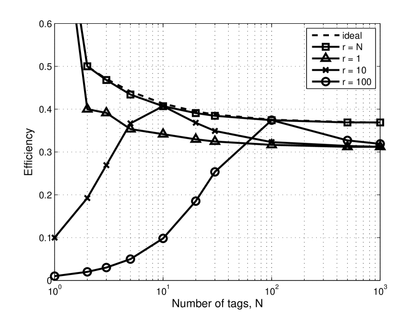
Figure 1: Efficiency versus the initial number of tags N of Schoute’s DFA mechanism for different values of the initial frame length $r$.

In Fig. 1 the efficiency for different values of $N$ with initial frame length $r_{0}=N$, $r_{0}=1$, $r_{0}=10$ and $r_{0}=100$ is shown. Values up to $N=30$ have been evaluated using (1), whereas values for $N=500$ and $N=1000$ have been obtained by simulating the algorithm. To allow comparisons we have also reported the performance with a perfect estimate $\hat{n}=n$ (dashed line), that represents a benchmark for all estimation mechanisms. We have also reported the case where only the estimate of the first frame is perfect, i.e. when the first frame length is set to $N$. The comparison of the latter cases shows that Shoute’s mechanism is able to track the backlog quite well if compared to the perfect estimate case, asymptotically reaching the best possible efficiency $e^{-1}$. In all the other cases, Schoute’s estimates suffer the mismatch between $N$ and the initial frame length $r$, and the efficiency degrades monotonically when $N$ increases beyond $r$, indicating the existence of a possible asymptote well below $e^{-1}$. The reasons for such behavior are analyzed next.

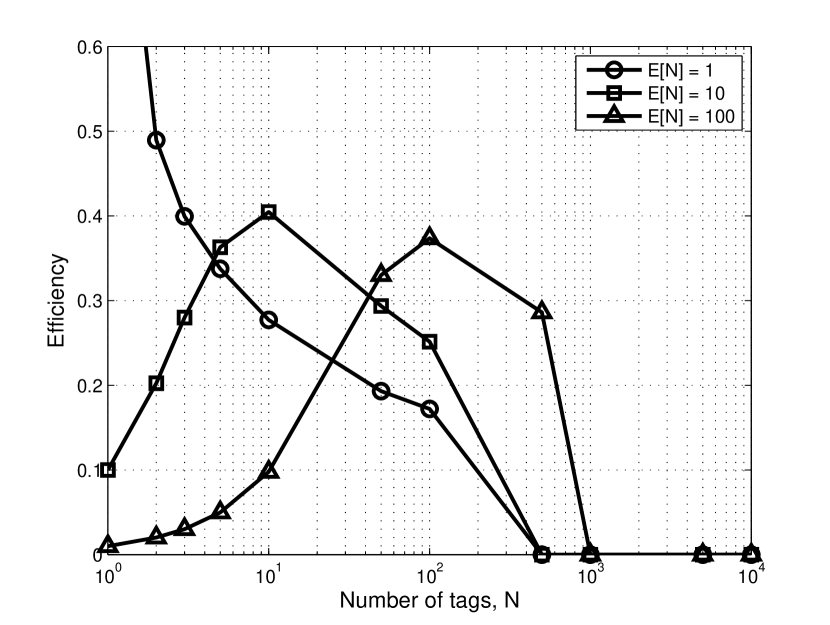
Figure 2: Efficiency of DFA with Bayes estimate and Poisson population-size distribution.

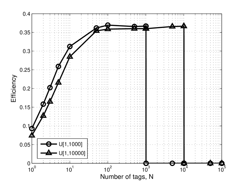
Figure 3: Efficiency of DFA with Bayes estimate and Uniform population-size distribution.

Figure 2 shows the efficiency of the Bayesian method when the population size distribution is Poisson with different averages. We see that the efficiency is optimal only when $N$ lies around the average. In all cases, when $N$ increases beyond some maximum value the efficiency drops to zero, meaning that the estimate converges to a constant value well below the actual value, so that successes are very rare. In Fig. 3 the performance with a uniform population size shows a similar behavior.

None of the two methods just shown seems to behave well asymptotically; however, the Schoute’s method is by far the simplest of the two and presents characteristics, namely the ability to remain locked to the true value, that suggest that it can be improved to reach maximum asymptotic efficiency. To this purpose, we present in the next section an asymptotic analysis that suggests how to reach the target.

III Asymptotic analysis of Schoute’s method

In the following analysis we assume that $N$ is very large, since we are interested in investigating the efficiency for $N\rightarrow\infty$. To facilitate the reader, we proceed in steps. In the remainder of the paper lower case letters represent random variables, whereas calligraphic upper cases represent averages.

Step 1. Here we derive recursive formulas for the backlog. We initially assume that the frame size $r_{i}$, and the backlog $n_{i}$ are so large that the number of transmissions in a slot can be approximated by a Poisson distribution with average $n_{i}/r_{i}$. This allows to evaluate the probability of an empty, successful and collided slot as

$$p_{e}=e^{-n_{i}/r_{i}};\qquad p_{s}=\frac{n_{i}}{r_{i}}e^{-n_{i}/r_{i}};\qquad p_{c}=1-\frac{n_{i}}{r_{i}}e^{-n_{i}/r_{i}}-e^{-n_{i}/r_{i}}.$$

We note that relations above also hold when starting with small $r$, because in this case, being $N-i$ always very large, every slot is collided with probability one. In Appendix A we show that, in the conditions assumed, the ratio $k_{i}=n_{i}/r_{i}$ can be safely replaced by the ratio of the respective averages ${\cal K}_{i}={\cal N}_{i}/{\cal R}_{i}$, which is the traffic per slot. With this substitution the probabilities above are denoted by ${\cal P}_{e},{\cal P}_{s},{\cal P}_{c}.$ This means that the average number of collisions and the average backlog size can be expressed as

$${\cal C}_{i}={\cal R}_{i}{\cal P}_{c},\qquad{\cal N}_{i+1}={\cal N}_{i}(1-{\cal P}_{s}).$$ (2)

The frame length evolves with law $r_{i+1}=\operatorname{round}(Hc_{i})$, so that

$${\cal R}_{i+1}=\operatorname{\mathbb{E}}\left\{\operatorname{round}(Hc_{i})\right\},$$ (3)

where $\operatorname{\mathbb{E}}\{\cdot\}$ is the expectation operator. Equations (2) and (3) form a recursion that provides sequences $\{{\cal R}_{i}\}$ and $\{{\cal N}_{i}\}$ that determine the efficiency. Unfortunately the rounding operation in (3) makes their analysis practically unfeasible.

Step 2. When $c_{i}$ is large, exploiting the limit $\lim_{x\rightarrow\infty}\operatorname{round}(x)/x=1$, we can replace $\operatorname{round}(Hc_{i})$ in (3) with $Hc_{i}$, obtaining

$${\cal R}_{i+1}=\operatorname{\mathbb{E}}\left\{\operatorname{round}(Hc_{i})\right\}\simeq H\operatorname{\mathbb{E}}\left\{c_{i}\right\}=H{\cal C}_{i}.$$ (4)

If we use (4) in the recursion in place of (3) we get sequences

$$R_{i+1}=HR_{i}\left(1-K_{i}e^{-K_{i}}-e^{-K_{i}}\right),$$ (5)

$$N_{i+1}=N_{i}\left(1-e^{-K_{i}}\right),$$ (6)

$$K_{i+1}=K_{i}\ \frac{1}{H}\frac{1-e^{-K_{i}}}{1-K_{i}e^{-K_{i}}-e^{-K_{i}}},$$ (7)

that correspond, respectively, to sequences $\{R_{i}\}$, $\{N_{i}\}$, and $\{K_{i}\}$. Later on we prove that replacing $\{{\cal R}_{i}\}$, $\{{\cal N}_{i}\}$, and $\{{\cal K}_{i}\}$ with the above sequences has no effect on the evaluation of the asymptotic performance. Also we prove that this holds even for finite values of the initial frame size $r_{0}$. In practice, we find that sequence $\{R_{i}\}$ approximates fairly well sequence $\{{\cal R}_{i}\}$, even for moderate values of $N$, and this allows recurrence (7) to be used in practice to evaluate the performance.

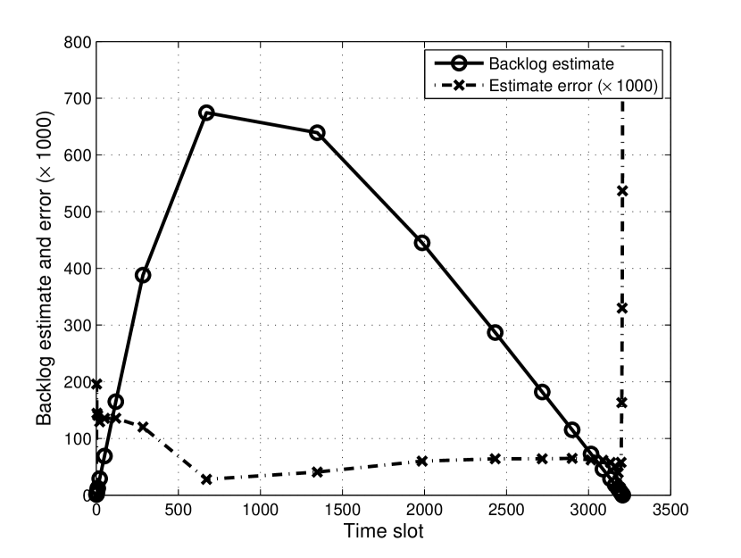
Figure 4: Average Schoute’s backlog estimate $\hat{\cal N}_{i}$ at the end of the frames versus time slot ($N=1000$, $r=1$). The dash-dotted line represents the relative error $\times 10^{3}$ with respect to the analytical values $N_{i}$.

As an example, Fig. 4 shows sequence $\{{\cal N}_{i}\}$ derived by averaging $10^{4}$ simulation samples in the case $N=10^{3}$ and $r_{0}=r=1$. We can clearly see a first phase where the estimate increases in order to converge to the true value $N=10^{3}$. In a second phase, optimal conditions are met, collisions are solved and the backlog decreases steadily to reach zero at about the 25-th iteration. We explicitly note that in the descending phase the rate of descent is $e^{-1}$, showing that Schoute’s algorithm is capable to correctly track the backlog and to solve contentions in the most efficient way. Figure 4 also shows the relative error sequence $\{({\cal N}_{i}-N_{i})/{\cal N}_{i}\}$ multiplied by $10^{3}$ (dash-dotted line). The error is always very small except at the end of the process, where ${\cal N}_{i}$ becomes small and ignoring the rounding effect is no longer appropriate. However, this error has no effect on the efficiency since it occurs for a small period of time, negligible when compared to the entire collision resolution length.

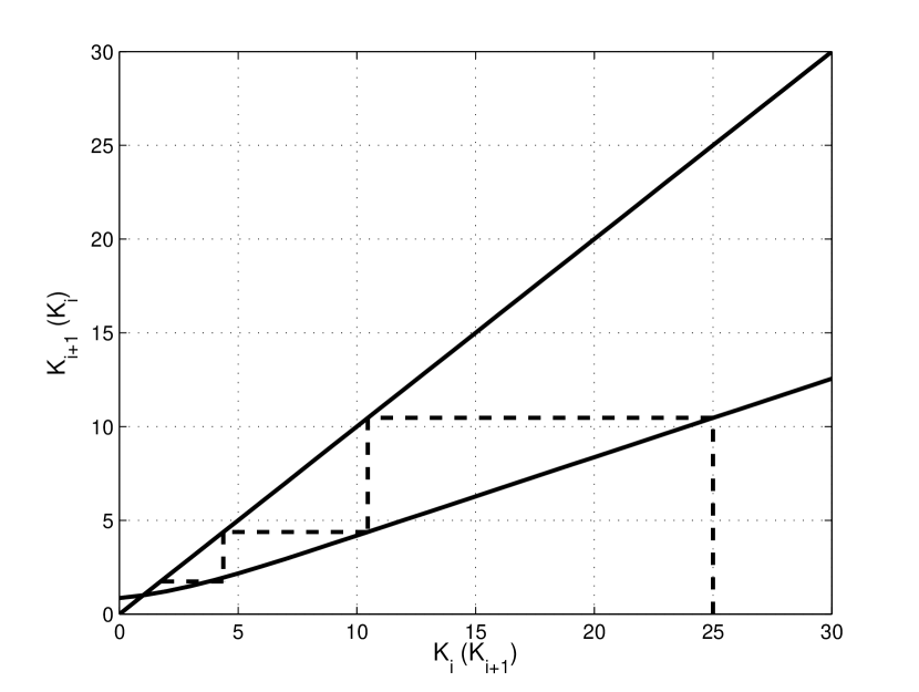
Figure 5: Representation of the trajectory of the sequence $\{K_{i}\}$.

Step 3. The evolution of the entire process is represented by recurrence (7) that depicts the evolution of average traffic $K_{i}$. This can be represented by the dashed trajectory in Fig. 5. This figure also shows that the evolution of the process is asymptotically stable since recurrence (7) leads to the fixed point in $K_{i}=1$. This point is also a point of optimality because in here we attain the optimal condition $r_{i}=n_{i}$ that provides maximum throughput.

When the starting point in (7) is $K=K_{0}=1$, the collision resolution process proceeds with a correct backlog estimate, yielding $K_{i}=1$, for all subsequent $i$ and we have

$$R_{i+1}=(1-e^{-1})R_{i},\qquad i\geq 0.$$ (8)

The solution of the recurrence (8) is $R_{i}=(1-e^{-1})^{i}N$, for $i\geq 0$. The total number of slot in this resolution phase is $L(N)=\sum_{i=0}^{\infty}R_{i}=Ne$, yielding an asymptotic throughput $N/L(N)=e^{-1}$. When $K=N/r>1$, the length of the entire procedure can be evaluated as $L(K)=\sum_{i=0}^{\infty}R_{i}=r\sum_{i=0}^{\infty}a_{i}$, with $R_{0}=r$, where sequence $\{a_{i}=R_{i}/r\}$ is always the same, for a given $K$, whichever $r$ is. Therefore, the efficiency is evaluated as $N/L=K/\sum_{i=0}^{\infty}a_{i}$ and only depends on $K=N/r$.

Step 4. Here we show that for large values of initial traffic $K$ the dependence of the efficiency on $K$ is negligible. Since the protocol always starts with a finite $r$, large $N$ means large $K$, so we attain practically the same efficiency whichever the initial frame length $r$ is.

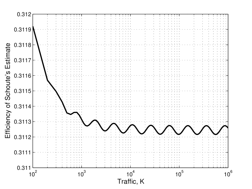
Figure 6: Efficiency of Schoute’s backlog estimate versus initial traffic $K$.

As an example, in Fig. 6 we have reported the efficiency $N/L(N)$, evaluated through (5) and (7), for different values of traffic $K$. Starting from $K=1$ the efficiency at first decreases as $K$ increases until about $K=500$ where it begins to oscillate without reaching an asymptote, around a mean value of $0.31125$, with a period that increases geometrically with $H$.

To attain some insight on the asymptotic behavior, during the solving process we consider three phases. The first phase, the approaching phase, starts at frame $0$ with infinite traffic and ends at frame $u$ where $u$ is chosen in such a way that the traffic $K_{u}$ is finite and practically no successes occur up to frame $u$; as an example we may arbitrarily assume $u$ such as $K_{u}\geq 10$. Although in this way $K_{u}$ and $u$ appear arbitrarily defined, we show below that this has no effect on the evaluation of the efficiency, as, in fact, the initial traffic $K$ has no effect. The assumed definition for $u$ assures that $u\rightarrow\infty$ as $N\rightarrow\infty$ and $R_{u}=N/K_{u}$.

The second phase, the convergence phase, starts at frame $u+1$ and ends at frame $u+v$ such that $K_{u+v}\simeq 1$. At this point the third phase, the tracking phase, begins where tags are solved with efficiency $e^{-1}$. Denoting by $L^{\prime},L^{\prime\prime}$, and $L^{\prime\prime\prime}$ the length of the three phases respectively, the efficiency is evaluated as $N/L(N)=N/(L^{\prime}+L^{\prime\prime}+L^{\prime\prime\prime})$.

With high values of $K=N/r$, in the first phase the frame length increases deterministically with law $R_{i}=rH^{i}$, for $i\geq 0$. The average number of slots up to frame $u$ where the first phase ends is

$$L^{\prime}=\sum_{i=0}^{u}R_{i}=r\frac{H^{u+1}-1}{H-1}\simeq\frac{H}{H-1}R_{u}.$$

Replacing $R_{u}=N/K_{u}$, the average length of the first phase becomes

$$L^{\prime}=\frac{H}{H-1}\frac{N}{K_{u}}=NA(K_{u}).$$

where $A(K_{u})$ is the proportionality constant where we have made explicit the dependence on $K_{u}$. The second phase starts at frame $u+1$, when $K_{u}$ is such that the collision probability is practically one, and ends at frame $u+v$ when $K_{u+v}\simeq 1$. Equation (5) can be used to evaluate the length of phase two by the following sum over a finite number of terms:

$$L^{\prime\prime}=\sum_{j=1}^{v}R_{u+j}=R_{u}\sum_{j=1}^{v}\alpha_{j}=NB(K_{u}),$$

where terms $\alpha_{j}$ are all finite and, again, where $B(K_{u})$ is the proportionality constant where we have made explicit the dependance on $K_{u}$. The average backlog size at the end of the second phase can be evaluated by (6) as

$$N^{\prime\prime}=N_{u+v}=N_{u}\prod_{j=1}^{v}\left(1-e^{-K_{u+j}}\right)=NC,$$

where we have exploited the fact that $N_{u}=N$. Coefficient $C$ does not depend on $K_{u}$, since in frame $u+1$ we still have all collisions ($e^{-K_{u+1}}\simeq 0$).

The third phase presents efficiency $e^{-1}$ and its average length is $L^{\prime\prime\prime}=N^{\prime\prime}e=NCe$. The efficiency with very large $N$ is then

$$\frac{N}{L(N)}=\frac{N}{L^{\prime}+L^{\prime\prime}+N^{\prime\prime}e}=\frac{1}{A+B+Ce}.$$ (9)

We note that (9) does not depend on the choice of $v$, once the condition $K_{u+v}\simeq 1$ is assured. If we replace $v$ by $v+1$, coefficient $A$ is not affected, and also term $B+Ce$ is not affected. In fact, $B$ is augmented by the term $R_{u+v+1}$ which, by (5) with $K_{u+v+1}\simeq 1$, is equal to

$$R_{u+v+1}=N_{u+v}(1-e^{-1}).$$ (10)

On the other side, term $Ce$ is diminished by $(N_{u+v}-N_{u+v+1})e=N_{u+v}(1-e^{-1})$, that is equal to term (10). Nevertheless, efficiency (9) does depend on the choice of $K_{u}$, through coefficients $A$ and $B$. However, if we replace $K_{u}$, chosen as suggested above, with $K_{u}\cdot H$, efficiency (9) does not change because this only implies the shifting of term $R_{u}$ from term $A$ to term $B$. Therefore, the efficiency is periodic in a logarithmic scale and all the asymptotic amplitudes of the oscillations in Fig. 6 can be obtained by replacing $K_{u}$ with any value $K^{\prime}$ in the range $(K_{u},HK_{u})$.

Table I shows the efficiency attained by (9) for different values of $K_{u}$ chosen in the range $(20,20H)$. As we can see, the values fit very well to those shown in Fig. 6 and, for all practical purposes, the asymptotic efficiency can be assumed equal to $0.311$.

Step 5. Now we show that replacing $L^{\prime},L^{\prime\prime}$, and $L^{\prime\prime\prime}$, in the limit $r\rightarrow\infty$, with $\mathcal{L^{\prime}},\mathcal{L^{\prime\prime}}$, and $\mathcal{L^{\prime\prime\prime}}$, in which the rounding operation is taken into account, does not change the results provided that the initial frame length is still $r$. In Appendix B we show that

$$\lim_{r\rightarrow\infty}\frac{\mathcal{L^{\prime}}(N)}{L^{\prime}(N)}=\frac{\sum_{i=0}^{\infty}\mathcal{R}_{i}}{\sum_{i=0}^{\infty}R_{i}}=1.$$

We also have $\lim_{r\rightarrow\infty}\mathcal{L^{\prime\prime}}(N)/L^{\prime\prime}(N)=1$, because the second phase is composed of a finite number $v$ of frames, each of them so large that the rounding effect is negligible. What shown also implies that at the end of the second phase we have $\lim_{r\rightarrow\infty}\mathcal{N}_{i}/N_{i}=1$, and, therefore, since those tags are solved with efficiency $e^{-1}$, also for the length of the third phase we have $\lim_{r\rightarrow\infty}\mathcal{L^{\prime\prime\prime}}(N)/L^{\prime\prime\prime}(N)=1$.

Step 6. If $r$ is small and (4) can not be assumed, the first phase is split into two sub-phases in which the second sub-phase starts at frame-index $x$ such that, from this frame onward, the rounding operation in (3) can be disregarded. Index $x$ is finite and the length of the first sub-phase does not depend on $N$, whereas the length of the second sub-phase and of the other phases is proportional to $N$. Therefore, as $N\rightarrow\infty$, the length of the first sub-phase vanishes and the asymptotic efficiency remains approximately $0.311$ even with small $r$.

IV An Asymptotically Efficient Estimation Procedure

The analysis of Schoute’s estimate carried out in the previous section has shown that the reduction of the asymptotic efficiency with respect to the theoretical value $e^{-1}$, when starting with a finite estimate, is not due to an intrinsic inefficiency of the estimate, but rather to the phase in which traffic $K$ converges to $1$, that is the convergence phase composed of $L^{\prime}$ and $L^{\prime\prime}$, whose length increases linearly with $N$. In particular, the length of this phase increases linearly with $N$ because the frame length increases exponentially as $H^{i}$, and this, from the overhead point of view, is a complete waste of time, since in this phase almost no success occurs. On the other side, the frame increase is needed to reduce the traffic per slot and get locked to the optimal point $K=1$. To get a good estimate of traffic $K$, we need not to explore the entire frame or, in another view, we need not to let all tags transmit in the frame; therefore, during the approaching phase toward $K=1$ the frame can be shorter and provide a convergence phase with an average length $L^{\prime}+L^{\prime\prime}$ such that

$$\lim_{N\rightarrow\infty}\frac{L^{\prime}+L^{\prime\prime}}{N}=0.$$ (11)

A way to reduce the number of tags transmitting in the frame is to specify at the beginning of the frame the transmission probability, together with the frame length. An alternative way, that is entirely compatible with the EPC standard, is to let all tags chose a slot in the frame, as in normal operation, but re-starting a new frame before the exploration of the entire frame is completed. Therefore, if we call virtual frame, of length $z$, the frame in which all tags select a slot for transmission, and real frame, of length $r\leq z$, the frame that has been explored when the frame is re-started, the traffic per slot $n/z$ is determined by the virtual frame, but only the real frame is observed and used to determine $\hat{n}$.

The estimation procedure we present in this section, the AE², adopts a virtual frame whose length $z_{i}$ is set equal to the backlog estimate $\hat{n}_{i}$, as it happens in the Schoute’s mechanism. Furthermore, the real frame length $r_{i}$ is set so that, in the convergence phase, it increases with index $i$ far less than the virtual frame length. As in DFA, backlogged terminals choose a slot in the virtual frame length $z_{i}$ and transmit in it only if the chosen slot belongs also to the real frame, i.e., if the Frame Restart command has not arrived yet. By setting a suitable law for $r_{i}$, the length of the first two phases can be easily forced to obey (11).

The backlog estimate is updated as follows

$$\left.\begin{array}[]{ll}z_{i+1}&=\hat{n}_{i+1}=\operatorname{round}\displaystyle\left(H_{i}\frac{z_{i}}{r_{i}}c_{i}\right),\qquad c_{i}>0,\\ z_{i+1}&=z_{i}-s_{i},\qquad c_{i}=0.\end{array}\right.$$ (12)

Update (12) is a variation of Schoute’s algorithm. It uses the number of collided slots $c_{i}$ in the real frame to get an estimate, $(z_{i}/r_{i})c_{i}$, of the number of collided slots in the virtual frame, multiplied by the factor $H_{i}$. When $c_{i}=0$, however, no estimate can be inferred by the observation, and, therefore, the estimate is assumed identical to the one in the previous frame diminished by the observed number of successes $s_{i}$. In Schoute’s work, where the algorithm is supposed to operate in $K=1$, we have $H_{i}=H$, for all $i$; in our case, however, such a setting cannot guarantee the convergence to $K_{i}=1$. This issue is discussed in Sec. IV-A.

As for the length of the real frame $r_{i}$, we asymptotically use the law

$$r_{i}=\min\{\operatorname{round}((i+1)^{b}),{z_{i}}\},$$ (13)

with $b>0$. In (13), with large $N$, with the exception of the first few slots, the real frame size increases, at first, as $(i+1)^{b}$, and later, when $z_{i}$ stabilizes and $i$ is such that $\operatorname{round}((i+1)^{b})>z_{i}$, the real frame coincides with the virtual one and the procedure becomes the classic DFA.

The proposed procedure resembles in some aspects the one in [14], where the traffic is decoupled from the frame length by the introduction of a frame transmission probability less than one. However, unlike our proposal where estimation takes place within the identification phase, in [14] the identification phase is preceded by an estimation phase, introduced ad hoc, whose length increases as $\log N$ and depends on the length of the estimate confidence interval, that must be made quite small, as no estimation is operated during the identification phase. The latter characteristic can jeopardize the procedure since no certainty exists to identify all tags.

IV-A Asymptotic Analysis of AE²

The analysis here presented is much the same as the one presented in Sec. III. Therefore we limit our explanation to parts that differ. Adopting the same assumptions used in Sec. III we can write the recursions corresponding to (5)-(7) as

$$Z_{i+1}=Z_{i}\ H_{i}\left(1-K_{i}e^{-K_{i}}-e^{-K_{i}}\right)$$ (14)

$$N_{i+1}=N_{i}\left(1-\frac{R_{i}}{Z_{i}}e^{-K_{i}}\right)$$

$$K_{i+1}=K_{i}\ \frac{1}{H_{i}}\frac{\displaystyle 1-\frac{R_{i}}{Z_{i}}e^{-K_{i}}}{1-K_{i}e^{-K_{i}}-e^{-K_{i}}}.$$ (15)

The key recursion (15) is different from (7) since now it also depends on $Z_{i}$ which complicates the matter. Since, for an efficient estimation we want $K_{i}$ to converge to $1$, sequence $\{H_{i}\}$ must be chosen as

$$H_{i}=\frac{\displaystyle 1-\frac{R_{i}}{Z_{i}}e^{-1}}{1-2e^{-1}}.$$ (16)

Recursion (15) is stable because it presents a unique fixed point in $K=1$ and we have

$$-1<\left.\frac{\partial}{\partial K}\left\{K\ \frac{1-2e^{-1}}{1-Be^{-1}}\ \frac{1-Be^{-K}}{1-Ke^{-K}-e^{-K}}\right\}\right|_{K=1}<1,$$

for all $B\in(0,1].$ Although values (16) could be evaluated a priori, in practice we can assume

$$H_{i}=\frac{\displaystyle 1-\frac{r_{i}}{z_{i}}e^{-1}}{1-2e^{-1}}.$$

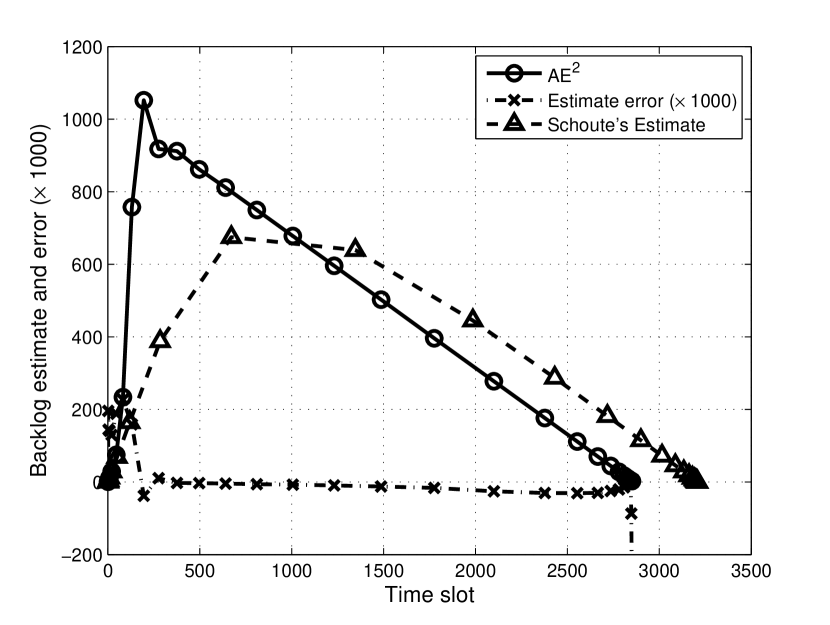
Figure 7: Average backlog estimate $\hat{\cal N}_{i}$ at the end of frames versus time slot, for the AE² algorithm ($N=1000$, $r=1$, $b=2$). The dash-dotted line represents the relative error $\times 10^{3}$ with respect to the analytical values $N_{i}$.

Figure 7 validates the analysis so far carried out. In fact, it compares the results the analysis produces in terms of sequence $\{{\cal N}_{i}\}$ with exact values attained averaging $10^{4}$ simulation samples, in the case $N=10^{3}$ and $r=1$. Again, the dash-dotted line represents the relative error multiplied by $10^{3}$, still very small. For comparison purposes we have also reported the curve in Fig. 4 that refers to Schoute’s algorithm. We clearly see the advantage of AE²: the estimate $\hat{\cal N}_{i}$ at first rises sharply reaching $N$ with some overshoot, higher and sooner with respect to Schoute’s case. Right after the estimate begins a steady decline with rate $e^{-1}$.

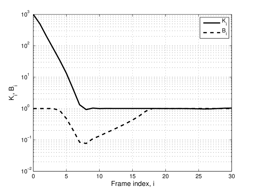
Figure 8: Sequences $\{K_{i}\}$ and $\{B_{i}\}$ versus the frame index $i$ ($N=1000$, $r=1$, $b=2$).

What stated above is confirmed in Fig. 8 where we have reported sequences $\{K_{i}\}$ and $\{B_{i}\}=\{R_{i}/Z_{i}\}$. The former shows the convergence of the estimate in $K=1$, while the latter reports the convergence of the real frame $R_{i}$ to the virtual frame $Z_{i}$. The protocol starts with $r_{0}=z_{0}$, $e^{-K_{i}}\simeq 0$ and subsequently we have $H\simeq 2.39$ as in Schoute’s, which yields $z_{1}=r_{1}=2$. Condition $r_{i}=z_{i}$ is maintained up to $i=3$ and then becomes $z_{i}>r_{i}$. $B_{i}$ decreases and when $r_{i}\ll z_{i}$ we have $H_{i}=H^{\prime}\simeq 1/(1-2e^{-1})\simeq 3.78$, and $z_{i+1}=H^{\prime}z_{i}$, reducing the traffic more quickly than in Schoute’s and speeding up the convergence phase, which is further reduced in time because the real frame is by far shorter. $B_{i}$ reaches a minimum when $K_{i}$ reaches one. At this point the real frame is so short that the collision solved are still very few. Beyond this point the protocol solves collisions with efficiency $e^{-1}$, $z_{i}$ decreases and $r_{i}$ increases until condition $r_{i}=z_{i}$ is reached again and never abandoned. From this point onward the backlog is solved exactly as in Schoute’s algorithm.

It is worth noting that the recursion in $B$ does not get into its fixed point $B=0$. In fact, once $K=1$ is reached, by (14) we can write $B_{i+1}/B_{i}=R_{i+1}/R_{i}(1-B_{i}e^{-1})^{-1}>1$.

Now we prove that the efficiency of AE² equals $e^{-1}$. The efficiency can be evaluated by writing, as in Sec. III,

$$\eta=\lim_{N\rightarrow\infty}\frac{N}{L^{{}^{\prime}}(N)+L^{{}^{\prime\prime}}(N)+N^{{}^{\prime\prime}}e},$$ (17)

where $L^{{}^{\prime}}(N)$ is the average number of slots of the first phase in which there are no successes, $L^{{}^{\prime\prime}}(N)$ is the average number of slots of the second phase in which the estimate of the backlog converges to the actual backlog. As it has been already observed, in the first phase we have $H_{i}=H^{\prime}$, so that we have $Z_{i}=r(H^{\prime})^{i}$, and assuming, as in the earlier analysis, that the first phase ends at frame $u$, where $Z_{u}=N/K_{u}$, solving the expression of $Z_{u}$ we get

$$u(N)=\log_{H^{\prime}}\frac{N}{rK_{u}}.$$ (18)

The length of this phase can be bounded as

$$L^{{}^{\prime}}(N)\leq\sum_{i=1}^{u(N)}i^{b+1}\leq\int_{0}^{u(N)+1}i^{b+1}\ di=\frac{(u(N)+1)^{b+2}}{b+2}\leq\frac{\left(1+\log_{H^{\prime}}\frac{N}{rK_{u}}\right)^{b+2}}{b+2},$$ (19)

where last inequality follows by (18), therefore we have $\lim_{N\rightarrow\infty}L^{{}^{\prime}}(N)/N=0$. The overhead of the second phase can be rewritten as

$$L^{{}^{\prime\prime}}(N)=(N-N^{{}^{\prime\prime}})(e-\epsilon),\qquad 0<\epsilon<e,$$ (20)

where $N^{{}^{\prime\prime}}$ is the backlog size at the end of the second phase. At the end of the first phase we have

$$B_{u}\triangleq\frac{R_{u}}{Z_{u}}\approx\frac{K_{u}u^{b}}{N}=\frac{K_{u}(\log_{H^{\prime}}N-\log_{H^{\prime}}rK_{u})^{b}}{N},$$

which implies $\lim_{N\rightarrow\infty}B_{u}=0$. In the second phase a few frames, $v$, are necessary to obtain $K=1$, and we still have $\lim_{N\rightarrow\infty}B_{u+v}=0$, which means that also the fraction of solved tags is asymptotically zero. Therefore, in (17) we have $\lim_{N\rightarrow\infty}N^{{}^{\prime\prime}}/N=1$, and by (20) $\lim_{N\rightarrow\infty}L^{{}^{\prime\prime}}(N)/N=0$, so that (17) yields $\eta=e^{-1}$.

V Practical Issues

V-A Overall Optimization

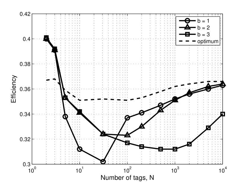
Figure 9: Efficiency of AE² and of overall optimization algorithms versus the tag population size $N$ for different values of parameter $b$.

The analysis carried out in the previous section shows that AE² is asymptotically efficient whatever the values of parameters in (13) are. Here we investigate the efficiency when $N$ is finite, in the range $[1,10000]$. Figure 9 shows the efficiency of the AE² procedure for three different values of the parameter $b$, versus the number of tags $N$ to be identified. We see that in all cases the convergence is assured, although with different performance. In fact, the best convergence is provided by $b=1$, because it reduces the approaching phase overhead as predicted by (19). We see, however, that for values of $N\leq 100$, the performance appears to deteriorate in all cases, because of the small length of the observed frame $r_{i}$, which increases the estimation variance.

The above observation shows that laws (13) and (12), though asymptotically optimal, are non-optimal with finite $N$. On the other side, those laws can be changed in a largely arbitrary way without affecting the asymptotic efficiency, as long as the former increases no more than polinomially, and the latter is an increasing function ultimately converging to (12). In the following we show a heuristic method to select those laws optimally, i.e., in such a way to provide nearly optimum performance for any $N$.

In the sequel we refer to a mechanism that subdivides the procedure into two phases, namely the approaching phase, that is roughly composed of the approaching phase and the converging phase defined in Sec. III, and the tracking phase. In the approaching phase we adopt, instead of (13) and (12), laws optimally determined for this phase, and afterward we turn to (13) and (12), thus assuring the convergence of $\hat{n}$ and the asymptotic optimality. We can not precisely define when the approaching phase finishes, since $\hat{n}$ gets close to $N$ but can rarely match it exactly. However, as the estimation mechanism of AE² becomes effective when not all collisions are observed in the frame, we reasonably assume that the approaching phase finishes at the frame that shows the first non collided slot.

In looking for optimal laws for the approaching phase, we are able to show that the two of them can be optimized separately. We assume at first that the estimate $\hat{n}$ (second law) is doubled at each frame. The performance indexes of the approaching phase are given by its overhead, that increases as the length of the real frame increases, and the accuracy of the approach of $\hat{n}$ to $N$, that can be measured by the traffic per slot $N/z_{i}=N/\hat{n}_{i}$, at the end of the approaching phase.

We now compare two cases, the first where all the frames of the approaching phase obey $r_{i}=1$, and the second when $r_{i}=2$. In both cases the estimate $\hat{n}$ is doubled at each frame, and the approaching phase finishes when a non-collided slot is observed. Assuming that the traffic per slot is Poisson distributed, independently at each slot, an assumption that becomes more accurate as $N$ increases beyond a few decades, we can easily find the a posteriori traffic $s$ that maximizes the probability of observing a non collided slot preceded by a sequence of all collided slot. This traffic turns out to be $s_{1}=1.4$ and $s_{2}=1.85$ for the two cases considered above. Simulations with $N=100$ provides $\bar{s}_{1}\simeq 1.5$ and $\bar{s}_{2}\simeq 2$ with standard deviations respectively equal to $0.9$ and $1$, while with $N=10$ provides $\bar{s}_{1}\simeq 1.4$ and $\bar{s}_{2}\simeq 1.85$ with standard deviations respectively equal to $0.6$ and $0.7$. These results clearly show that the approach of the first case is slightly better, i.e., closer to $1$, than the second one. On the other side, increasing the frame length beyond one remarkably increases the overhead, so that the first case is definitely better than the second one. Based on this argument we may conclude that making

$$r_{i}=1,\qquad i\geq 0,$$ (21)

always provides close to best performance.

In general, the estimate update can be represented by the law

$$\hat{n}_{i+1}=H^{\prime}_{i}\hat{n}_{i}.$$ (22)

Repeating the above evaluations it appears that, as long as sequence $\{H^{\prime}_{i}\}$ is close to all twos, say in the range $[1.5;2.5]$, (21) is still optimal. We now look for the optimal $\{H^{\prime}_{i}\}$ within the cited range. Here, we define the optimum sequence as the one that yields the highest among the minimum efficiencies observed in the whole range of $N$, so that the efficiency curve turns out as flat as possible.

The problem simplifies in some ways. First, we observe that a sequence $\{H^{\prime}_{i}\}$ composed of all twos yields good performance above $N=1000$, while the minimum of the efficiency appears to be in the range $N<1000$. In this range, doubling $\hat{n}$ at each frame, provides an approaching phase length that in the majority of cases lasts about $10-12$ frames. This means that our optimum search can be limited to such a finite sequence. By further discretizing $H_{i}$ in steps of $0.1$, we have been able to perform an exhaustive search that yields as optimal multipliers the sequence

$$H=[2\ \ 2\ \ 2\ \ 2\ \ 1.8\ \ 1.7\ \ 1.7\ \ \ldots,1.7\ \ \ldots].$$ (23)

We have prolonged the above sequence beyond $i=12$ since this prolongation little, if at all, affects the results with high $N$. The corresponding efficiency curve is shown in Fig. 9 and positively compares with the curves seen before. Here, we can appreciate that the efficiency is always above $0.35$, reaching $e^{-1}$ asymptotically.

V-B Implementation issues

As we have already stated at the beginning of Sec. IV, real and virtual frames in AE² are compatible with the EPC standard set of commands. The procedure summarized in (12), (13), (21) and (23) can easily be performed in the reader. However, in this standard, the frame size (virtual, in our case), conveyed by the reader to tags, must be of the type $2^{Q}$, with $Q$ in the range from one to $16$. This constraint impairs the performance even if $N$ is known, since it prevents the optimal assignment $r=n$.

Here we expose an approximate argument that is able to capture the asymptotic impairment due to the replacement of the optimal frame length $n$ with the value closest to $2^{Q}$, when the backlog $n$ is known.

Denoting by $\{n_{i}\}$ and $\{r_{i}\}$ the sequence of backlogs and frame lengths, we assume that the random variable $n_{i}/r_{i}$, i.e., the average number of tags per slot in frame $i$, presents the same statistics regardless of the index $i$ of the frame, which can be considered a good approximation for a large part of frames when $N$ is very large. This leads to a frame efficiency $\eta_{f}$ equal for all frames and, therefore, the identification period length $L(n)$, starting with $n$ tags, can then be written as $L(n)=\sum_{i}r_{i}=n+n(1-\eta_{f})+n(1-\eta_{f})^{2}+\ldots=n/\eta_{f}$, where, as usual when $n$ is large, we have considered the random variables equal to their averages. This argument shows that the overall efficiency is $\eta=\eta_{f}$. In order to determine $\eta_{f}$, we find the statistics of $n_{i}/r_{i}$, when the power index $Q_{i}$ of the frame length is assumed such that $2^{Q_{i}}$ is the closest to $n_{i}$. To the purpose, let assume that such index is $Q_{i}=q$. This means that $n=n_{i}$ is in the range $[2^{q}-2^{q-2},2^{q}+2^{q-1}]$, being with equal probability higher or lower than $2^{q}$. Similarly, $s=n/r=n/2^{q}$ has a distribution that is bivariate, namely uniform within $[3/4,1]$ with probability $1/2$, and uniform within $[1,3/2]$ again with probability $1/2$. The efficiency, or probability of a slot being successful, can be expressed as $\left(1-1/r\right)^{n-1}=\left(1-s/n\right)^{n-1}\rightarrow e^{-s}$ and, averaged over the distribution of $s$ already cited, provides $\eta=\eta_{f}=0.3562$.

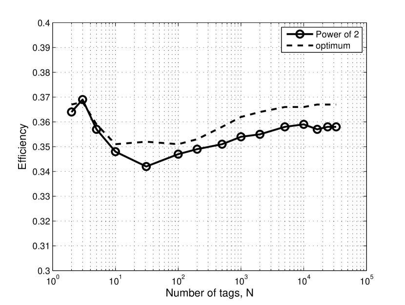
Figure 10: Efficiency of AE² and overall optimization algorithms versus the tag population size $N$ for different values of parameter $b$.

The above value of $\eta$ almost perfectly matches the asymptotic values we have found by simulation, namely $0.357$. Figure 10 shows the efficiencies of AE² and its constrained version. In the latter, sequence (23) has been replaced by a sequence of all $2$, whereas (12) is replaced by the closest $2^{Q}$. The results clearly show the impairment due to the constraint, but they also show that, also in the constrained version, our procedure is able to asymptotically reach the theoretical performance.

VI Conclusions

In this paper we have presented an asymptotic analysis of Schoute’s backlog estimate for DFA, applied to the RFID environment. The analysis shows that the asymptotic efficiency of this estimate is $0.311$, far less than the theoretical maximum $e^{-1}\approx 0.368$, achieved when the backlog is known. The analysis shows that the performance loss is due to the slow convergence of the estimate and suggests how this impairment can be avoided. Using these results we have introduced the AE², a procedure that asymptotically reaches the theoretical maximum, and that can be set to achieve an efficiency close to maximum for any finite value of the population size. We have also derived the asymptotic efficiency when the frame size is constrained to be a power of two, as required by RFID standards for DFA, with which the proposed protocol is fully compatible. Although the gain with existing mechanisms is moderate (in the $10-20\%$ range), we remark that the proposed procedure is able to cope with any tag number, and does not present an hard limit on the maximum number of tags to be resolved.

Appendix A

If $n_{i}$ and $r_{i}$ are both large, collided slots in frame $i$ become distributed according to a binomial distribution with average $r_{i}p_{c}$ and variance $r_{i}p_{c}(1-p_{c})$, which is upper bounded by $r_{i}$. Therefore, being, in the approaching phase and for large $r$, $r_{i+1}=Hc_{i}$ we have

$$\mbox{VAR}\{r_{i+1}|n_{i},r_{i}\}=H^{2}\ \mbox{VAR}\{c_{i}|n_{i},r_{i}\}\leq H^{2}r_{i}.$$ (24)

Since the number of collisions can not be larger than $N/2$ it follows that

$$r_{i}\leq H\frac{N}{2},$$ (25)

for all $i$. Substituting (25) into (24) yields $\mbox{VAR}\{r_{i+1}|n_{i},r_{i}\}\leq Nd$, where $d$ is a constant value. The Chebyshev’s inequality used with the above bound yields

$$\Pr(|r_{i+1}-{\cal R}_{i+1}|\geq\epsilon N|n_{i},r_{i})\leq\frac{d}{N\epsilon^{2}},$$

that can be reduced to

$$\Pr(|r_{i+1}-{\cal R}_{i+1}|\geq\epsilon N)\leq\frac{d}{N\epsilon^{2}}.$$ (26)

Relation (26) shows that, for $N\rightarrow\infty$, we have $r_{i}/N\rightarrow{\cal R}_{i}/N,$ where the convergence is in probability. Much in the same manner one can show that $n_{i}/N\rightarrow{\cal N}_{i}/N,$ and, therefore, we have $n_{i}/r_{i}\rightarrow{\cal N}_{i}/{\cal R}_{i}$ in probability.

Appendix B

Here we consider sequence $\{\mathcal{R}_{i}\}$ during the first phase, where all the slots are collided, i.e., $\mathcal{C}_{i}=\mathcal{R}_{i}$ and relation (3) becomes $\mathcal{R}_{i+1}=\operatorname{\mathbb{E}}\{Hc_{i}+\xi_{i}\}=H\mathcal{C}_{i}+\Xi_{i}=H\mathcal{R}_{i}+\Xi_{i}$, for $i\geq 0$. On the other side we have $R_{i+1}=HR_{i}$, for $i\geq 0$, with $\mathcal{R}_{0}=R_{0}=r$. Solving the recursions we get

$$\mathcal{R}_{i}=rH^{i}+\sum_{k=0}^{i-1}H^{i-1-k}\Xi_{k}$$ (27)

$$R_{i}=rH^{i},$$ (28)

for $i\geq 0$. Relation (27) can be rewritten as $\mathcal{R}_{i}=R_{i}+\sum_{k=0}^{i-1}H^{i-1-k}\Xi_{k}$. Since $|\Xi_{k}|\leq 0.5<1$, and being $\sum_{k=0}^{i-1}H^{k}=(H^{i}-1)/(H-1)$, we can write

$$R_{i}-\frac{H^{i}-1}{H-1}<\mathcal{R}_{i}<R_{i}+\frac{H^{i}-1}{H-1},\ \ \ \ \ \ i\geq 0,$$

and

$$1-\frac{f(H)}{r(H-1)}<\frac{\sum_{i=0}^{\infty}\mathcal{R}_{i}}{\sum_{i=0}^{\infty}R_{i}}<1+\frac{f(H)}{r(H-1)},$$

with $f(H)=(\sum_{i=0}^{\infty}(H^{i}-1))/(\sum_{i=0}^{\infty}H^{i})$, having exploited (28). Since it is $H^{i}-1<H^{i}$, for $i\geq 0$, we also have $f(H)<1$, and finally $\lim_{r\rightarrow\infty}(\sum_{i=0}^{\infty}\mathcal{R}_{i})/(\sum_{i=0}^{\infty}R_{i})=1$.

Table I: Analytical values of the asymptotic efficiency of DFA with Schoute’s estimate for different values of the parameter $K_{u}$.

$K_{u}=20$ $K_{u}=25$ $K_{u}=30$ $K_{u}=35$ $K_{u}=40$ $K_{u}=45$ $K_{u}=47.8$ $N/L(N)$ 0.31125 0.31127 0.31125 0.31122 0.31122 0.31123 0.31125

References

- [1] F. Schoute, “Dynamic frame length aloha,” Communications, IEEE Transactions on, vol. 31, no. 4, pp. 565 – 568, apr 1983.
- [2] K. Finkenzeller, RFID handbook: fundamentals and applications in contactless smart cards and identification. John Wiley & Sons, 2003.
- [3] Information technology Radio frequency identification for item management Part 6: Parameters for air interface communications at 860 MHz to 960 MHz, International Organization for Standardization Std., 2004.
- [4] Class 1 Generation 2 UHF Air Interface Protocol Standard Version 1.0.9, EPCglobal Std., 2005.
- [5] R. Rom and M. Sidi, Multiple Access Protocols. Springer-Verlag, 1990.
- [6] L. Barletta, F. Borgonovo, and M. Cesana, “A formal proof of the optimal frame setting for dynamic-frame aloha with known population size,” arXiv:1202.3914v2 (cs.IT).
- [7] C.-F. Lin and F.-S. Lin, “Efficient estimation and collision-group-based anticollision algorithms for dynamic frame-slotted aloha in rfid networks,” Automation Science and Engineering, IEEE Transactions on, vol. 7, no. 4, pp. 840 –848, oct. 2010.
- [8] L. Zhu and T.-S. Yum, “A critical survey and analysis of rfid anti-collision mechanisms,” Communications Magazine, IEEE, vol. 49, no. 5, pp. 214 –221, may 2011.
- [9] ——, “Optimal framed aloha based anti-collision algorithms for rfid systems,” Communications, IEEE Transactions on, vol. 58, no. 12, pp. 3583 –3592, december 2010.
- [10] H. Vogt, “Efficient object identification with passive rfid tags,” in Proceedings of the First International Conference on Pervasive Computing, ser. Pervasive ’02. London, UK: Springer-Verlag, 2002, pp. 98–113. [Online]. Available: http://portal.acm.org/citation.cfm?id=646867.706691
- [11] J.-R. Cha and J.-H. Kim, “Novel anti-collision algorithms for fast object identification in rfid system,” in Parallel and Distributed Systems, 2005. Proceedings. 11th International Conference on, vol. 2, july 2005, pp. 63 –67.
- [12] W.-T. Chen, “An accurate tag estimate method for improving the performance of an rfid anticollision algorithm based on dynamic frame length aloha,” Automation Science and Engineering, IEEE Transactions on, vol. 6, no. 1, pp. 9 –15, jan. 2009.
- [13] C. Floerkemeier, “Bayesian transmission strategy for framed aloha based rfid protocols,” in RFID, 2007. IEEE International Conference on, march 2007, pp. 228 –235.
- [14] M. Kodialam and T. Nandagopal, “Fast and reliable estimation schemes in rfid systems,” in Proceedings of the 12th annual international conference on Mobile computing and networking, ser. MobiCom ’06. New York, NY, USA: ACM, 2006, pp. 322–333. [Online]. Available: http://doi.acm.org/10.1145/1161089.1161126