Recurrent Coronal Jets Induced by Repetitively Accumulated Electric Currents

Abstract

Jets of plasma are frequently observed in the solar corona. A self-similar recurrent behavior is observed in a fraction of them. Jets are thought to be a consequence of magnetic reconnection, however, the physics involved is not fully understood. Therefore, we study some jet observations with unprecedented temporal and spatial resolutions. The extreme-ultraviolet (EUV) jets were observed by the Atmospheric Imaging Assembly (AIA) on board the Solar Dynamics Observatory (SDO). The Helioseismic and Magnetic Imager (HMI) on board SDO measured the vector magnetic field, from which we derive the magnetic flux evolution, the photospheric velocity field, and the vertical electric current evolution. The magnetic configuration before the jets is derived by the nonlinear force-free field (NLFFF) extrapolation. Three EUV jets recurred in about one hour on 2010 September 17 in the following magnetic polarity of active region 11106. We derive that the jets are above a pair of parasitic magnetic bipoles which are continuously driven by photospheric diverging flows. The interaction drove the build up of electric currents that we indeed observed as elongated patterns at the photospheric level. For the first time, the high temporal cadence of HMI allows to follow the evolution of such small currents. In the jet region, we found that the integrated absolute current peaks repetitively in phase with the 171 Å flux evolution. The current build up and its decay are both fast, about 10 minutes each, and the current maximum precedes the 171 Å by also about 10 minutes. Then, HMI temporal cadence is marginally fast enough to detect such changes. The photospheric current pattern of the jets is found associated to the quasi-separatrix layers deduced from the magnetic extrapolation. From previous theoretical results, the observed diverging flows are expected to build continuously such currents. We conclude that magnetic reconnection occurs periodically, in the current layer created between the emerging bipoles and the large scale active region field. It induced the observed recurrent coronal jets and the decrease of the vertical electric current magnitude.

1 Introduction

Solar jets are observed at many wavelengths, such as H$\alpha$, UV, EUV, and X-rays (Schmieder et al., 1988; Shibata et al., 1992a; Canfield et al., 1996; Chae et al., 1999; Uddin et al., 2012). They are called surges in cold spectral lines (e.g., H$\alpha$) and jets at other wavelengths, which indicates that both cold (e.g., Srivastava & Murawski, 2011; Kayshap et al., 2013) and hot plasma are accelerated in the jet phenomenon. Magnetic reconnection is widely accepted as the central physical mechanism. There are different magnetic reconnection models for coronal jets according to photospheric flow patterns and coronal magnetic topologies, for instance, the emerging flux model (Heyvaerts et al., 1977; Shibata et al., 1992b; Gontikakis et al., 2009; Archontis et al., 2010), the converging flux model (Priest et al., 1994), the Quasi-Separatrix Layer (QSL) model (Mandrini et al., 1996), and the null-point and fan-separatrix model (Moreno-Insertis et al., 2008; Török et al., 2009; Pariat et al., 2009, 2010). Moreno-Insertis et al. (2008) and Török et al. (2009) use emerging flux, while Pariat et al. (2009, 2010) use horizontal photospheric twisting motion to drive the magnetic reconnection in their simulations. Although some of the aforementioned models focus on solar flares and coronal bright points, the associated jet phenomenon has also been discussed.

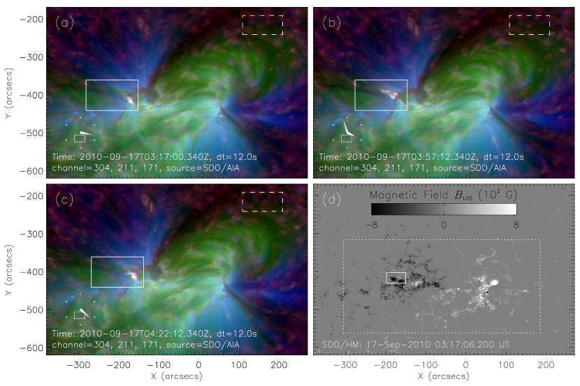
Figure 1: (a)–(c) SDO/AIA EUV composite images. Each EUV image consists of three channels (red, blue, and green) in the 304 Å, 171 Å, and 211 Å channels, whose characteristic temperature corresponds to 0.05 MK, 0.6 MK, and 2 MK, respectively. The larger solid box marks the jet region where the 171 Å fluxes are integrated. The smaller solid box on the clock indicates the position and field of view of the EUV image on the solar disk. The dashed box indicates the region where the background flux for the 171 Å band is computed. (d) SDO/HMI line-of-sight magnetic field. The black/white color represents the negative/positive polarity. The solid box marks the region of the foot-points of the jets, where the line-of-sight magnetic field flux is integrated. The dotted box marks the field of view for the analysis of the vector magnetic field.

H$\alpha$ surges and EUV/X-ray jets emanating from the same region tend to appear recurrently (Schmieder et al., 1995; Asai et al., 2001; Chifor et al., 2008; Wang & Liu, 2012; Zhang et al., 2012). The period ranges from tens of minutes to several hours. It is still not clear which physical mechanism accounts for the quasi-periodicity. Pariat et al. (2010) proposed a null-point and fan-separatrix model driven by the photospheric twisting motion. As a consequence of the continuous driving by photospheric motions, this model produces recurrent jets, which explains the quasi-periodicity. Zhang et al. (2012) proposed another possible mechanism that the null-point reconnection responsible for the quasi-periodicity is modulated by trapped slow-mode waves along the spine field lines, and slow-mode wave has been reported in, e.g., Cirtain et al. (2007). Both models consider magnetic topologies with null-points. But how to explain those events whose magnetic topologies are QSLs or bald patches? Moreover, the photospheric motion is believed to be the driver of these recurrent jets. Can we find any indicator of the quasi-periodicity from the photosphere, such as from the magnetic flux evolution, the velocity field, or the electric current evolution?

In this paper, we present three recurrent coronal jets that were observed on 2010 September 17 by the Atmospheric Imaging Assembly (AIA; Lemen et al. 2012) on board the Solar Dynamics Observatory (SDO). In order to find a clue on the magnetic reconnection model and the physical mechanism accounting for the quasi-periodicity, we study the EUV flux, the magnetic flux, the velocity field, and the vertical electric current evolutions. The vector magnetic fields are observed by the Helioseismic and Magnetic Imager (HMI; Scherrer et al. 2012; Schou et al. 2012b) on board SDO. Section 2 presents the data analysis and results. Discussion and conclusion are given in Section 3.

2 Data Analysis and Results

2.1 Jets Observed in EUV

SDO/AIA provides high cadence of 12 s, high spatial resolution of $1.5^{\prime\prime}$ (the pixel sampling is $0.6^{\prime\prime}$ per pixel), and high signal-to-noise observations nearly simultaneously in seven EUV lines, two UV continuums, and one white-light band. Figure 1 displays three composite EUV images showing that three coronal jets recurred on the border of active region (AR) 11106. All the EUV images have been aligned with “aia_prep.pro” in the Solar SoftWare (SSW). A line-of-sight magnetic field observed by SDO/HMI is displayed in Figure 1d as an example, which shows that some parasitic positive polarities distribute in the main negative polarities. SDO/HMI has a spatial resolution of $1^{\prime\prime}$ (the spatial sampling is $0.5^{\prime\prime}$ per pixel) and a cadence of 45 s for the line-of-sight magnetic field. It has also been aligned with the EUV images with “aia_prep.pro”.

We compute the EUV flux in the 171 Å band to give a quantitative representation of the evolution of the recurrent jets. The 171 Å flux is computed within a rectangle containing the full jet region as shown by the larger solid box ($130^{\prime\prime}\times 80^{\prime\prime}$) in Figure 1a–1c. We select two time ranges to compute the 171 Å flux evolution, i.e., a context range from 00:00 to 10:00 UT and a smaller analysis range centered on the analyzed jets from 03:00 to 05:00 UT. Due to the limitation of computation resources, the temporal resolution for the context range is 2 minutes and it is 12 seconds for the analysis range. The 171 Å flux evolutions for the two time ranges are plotted in Figures 2a and 2b, respectively. The data gap between 06:31 to 07:13 UT is due to the SDO eclipse by the Earth. We have normalized the 171 Å flux to its background level, which is computed in a quiet region as shown in the dashed box of Figure 1a–1c. The 171 Å background flux shows a flat curve (Figure 2a). Therefore, the variations in the 171 Å flux curve in the jet region are mainly due to the jets themselves, but not the background.

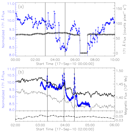
Figure 2: SDO/AIA 171 Å averaged and normalized flux and SDO/HMI line-of-sight magnetic flux. (a) Blue stars indicate the 171 Å flux in the jet region divided by the number of pixels in the box (larger solid box as shown in Figure 1a–1c) normalized to the background flux, which is computed in the dashed box shown in Figure 1. Plus signs represent the averaged background flux per pixel. The temporal resolution is about 2 minutes. The two vertical lines mark the time range for 171 Å flux as shown in the bottom panel. (b) The temporal resolution for the 171 Å flux is about 12 s. The three vertical lines mark the peak times of the 171 Å flux. Dash-dotted, dotted, and solid lines indicate positive, unsigned negative, and total unsigned line-of-sight magnetic flux, respectively.

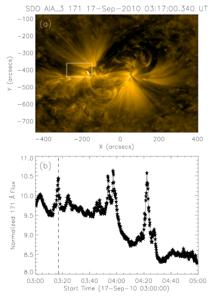
Figure 7: Online only figure. A movie showing the evolution of this figure from 03:00 to 05:00 UT is available in the online journal. (a) SDO/AIA 171 Å image. The box marks the region where the 171 Å fluxes are computed. (b) SDO/AIA 171 Å flux normalized to the background level, which is defined as the flux in the quiet Sun region (see Section 2.1 for more details). The vertical dashed line marks the time of the 171 Å image in panel (a).

Figure 2a shows many fluctuations or peaks in the 171 Å flux curve during the context range, which indicates that there are many brightening points or jets during this time range in the selected region. However, the peaks during the analysis range are more distinct than the others. Therefore, we select this time range for a detailed analysis. The 171 Å flux curve in Figure 2b has three main peaks at 03:17 UT, 03:57 UT, and 04:22 UT, respectively. There are some smaller peaks before the jet at 03:57 UT. Using the 171 Å movie (attached to the online-only Figure 7), we find that this jet consists of successive ejections during a short period. The other two events are relatively simple with only one ejection in each event.

2.2 Line-of-Sight Magnetic Flux Evolution

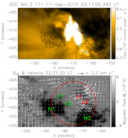
Figure 3: (a) SDO/AIA 171 Å image overlaid by the line-of-sight magnetic field observed at the same time as that of the 171 Å image. Gray/black lines mark the contour levels of the positive/negative polarities. The contour levels of $B_{z}$ are -1200, -900, -600, 300, and 600 G. (b) Map of photospheric transverse velocities derived from LCT analysis with the HMI magnetograms, employing a FWHM correlation window of $5^{\prime\prime}$ during the time interval 02:25–02:50 UT. Arrows represent velocities and the background is the line-of-sight magnetogram with positive (white) and negative (black) polarities. Black/white arrows are located on positive/negative polarities. North/south is up/down, west/east is towards right/left. The magnetic polarities involved in the jets are identified with annotations (p1 and p2 for parasitic positive, n1 and n2 for parasitic negative, while N0 and N1 for the main following negative polarities). The circle highlights the region of interest where the diverging flows are found. A movie showing the evolution of the line-of-sight magnetic field from 02:00 to 06:00 UT is available in the online journal.

Figure 2b displays the unsigned line-of-sight magnetic flux evolution. The line-of-sight magnetic flux is integrated in a small rectangle containing mainly the foot-points of the jets with a size of $48^{\prime\prime}\times 28^{\prime\prime}$ as shown by the solid box in Figure 1d. The box size for the 171 Å flux computation is larger than that for the magnetic flux because, on one hand, jets are events occupying areas in the corona that are more extended than the triggering magnetic field region in the photosphere below. On the other hand, the parasitic polarities involved with the jets are surrounded by main polarities of the active region, which would bias the computation of the line-of-sight magnetic flux if the box is too large. The positive magnetic flux increases from 02:00 to 03:00 UT and evolves almost steadily from 03:00 to 05:00 UT (Figure 2b, dash-dotted curve). The negative flux curve is dominated by the main negative polarity of the active region and some of the flux is close to the border of the selected region (Figure 1d), then, due to convective motions of the photospheric plasma, magnetic flux might be displaced and no longer captured by the selected area. For this reason, the unsigned negative flux evolution (Figure 2b, dotted curve) is not necessarily related to the jetting events. It evolves steadily from 02:00 to 03:00 UT and decreases during the recurrent jets from 03:00 to 05:00 UT. Comparing the magnetic flux evolution with the 171 Å flux evolution, we do not find a clear relationship between them. The unsigned magnetic flux in the negative polarity, either decreases (for the jets at 03:17 and 04:22 UT) or increases (for the jet at 03:57 UT) before a jet. There is also no significant evolution of the positive magnetic flux related to the jets. This result is coherent with a progressive storage of magnetic energy in the corona, reaching a critical point, and release part of the free magnetic energy without affecting the magnetic flux crossing the photosphere.

Figure 3a shows that the foot-points of the EUV jets are located where parasitic polarities appear, as follows. As shown in Figure 1d, AR 11106 consists of a leading positive and a following negative polarity, which has two strong concentrated polarities N0 and N1. The parasitic polarities noted as p1, p2, n1, and n2 in Figure 3b are present in the following negative polarity of AR 11106. The positive parasitic polarities p1 and p2 separate westward from the eastern negative polarity (n1 and n2). Polarities n1 and n2 have almost merged with the following main polarity N1 of AR 11106, while p2 is pushed against another part of the following main polarity (N0). The evolution of these polarities can be seen in the movie of the line-of-sight magnetic field attached to Figure 3 (available in the online journal).

We further study the transverse flows of photospheric magnetic features with local correlation tracking techniques (November & Simon, 1988, hereafter LCT). By using a Gaussian tracking window of full width at half maximum (FWHM) of $5^{\prime\prime}$, we compute the proper motions of magnetic elements over the SDO/HMI sequence of magnetograms. The window size of $5^{\prime\prime}$ is appropriate because it is large enough to contain the coherent structures to correlate, but not too large to keep as much as possible the spatial resolution and also to limit the computation time to feasible values. The time series used for this analysis starts at 02:00 UT on 17 September 2010 and is composed by 137 images with a cadence of 45 seconds. Images are grouped in 25-min series for the LCT analysis. Prior to applying LCT the sequence of images is aligned to eliminate possible jitter and rotation of the observed target within the field of view. Since the differential rotation is of minor influence here due to the small field of view, we do not remove this effect. Taking the first image as reference, the second image is aligned to it by correlating them. Then, the third image is aligned with the second one with the same method. The process is repeated until all the 137 images are aligned with each other. We find that the maximum shift is up to 21 pixels in the East-West direction and less than 1 pixel in the North-South direction. The absolute values of the transverse velocities should be taken with caution because the LCT technique in general produces some systematic errors in the determination of proper motions (November & Simon, 1988). The LCT method may underestimate 20%–30% of the velocities in extreme cases (Molowny-Horas, 1994). But it usually generates reliable flow patterns (November & Simon, 1988; Vargas Domínguez et al., 2008).

The results confirm the emergence pattern seen in the magnetic field movie. There is indeed a diverging flow with the polarities p1 and p2 moving mostly westward and their negative counterparts, n1 and n2, moving mostly eastward (this diverging flow pattern is, in average inclined by about $20^{\circ}$ on the East-West direction), while the bipoles n1-p1 and n2-p2 are mostly East-West oriented at that time.

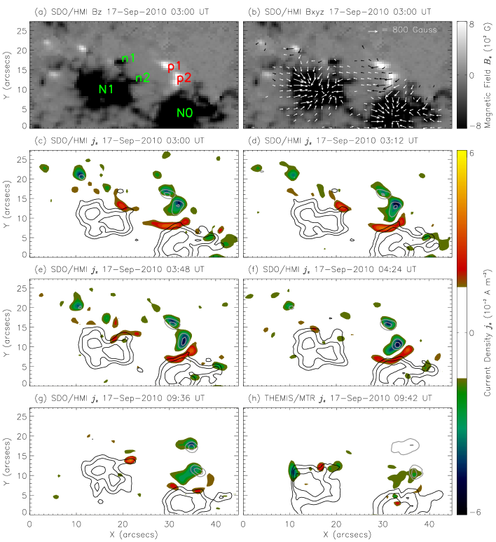
Figure 4: (a) SDO/HMI vertical component of the magnetic field ($B_{z}$). The projection effect is removed. (b) SDO/HMI vector magnetic field with the $180^{\circ}$ ambiguity being removed. (c)–(g) Distribution of the vertical electric current density $j_{z}$ averaged over 12 minutes at different times and observed by SDO/HMI. The middle time of the observations is indicated at the top of each panel. Gray/black lines mark the contour levels of the positive/negative polarities. The contour levels of $B_{z}$ are $-1200,-900,-600,300$, and $600$ G. The color bar of $j_{z}$ is shown on the right side. (h) Distribution of $j_{z}$ observed by THEMIS/MTR centered at 09:42 UT. The scan duration is about 16 minutes in this field of view. The contour levels of $B_{z}$ are $-882,-661,-440,110$, and $220$ G, which are at the same percentage of their minimum (for the negative contours) and maximum (for the positive contours) values as that in Figure 4g.

2.3 Vector Magnetic Field

We further analyze the vector magnetic fields observed by SDO/HMI, which records six filtergrams at each of six wavelengths every 135 s. The filtergrams at each wavelength correspond six polarization states, i.e., $I\pm S$, where $S=Q,U$, and $V$, where the notations $I,Q,U,$ and $V$ represent the four Stokes parameters. In order to increase the signal to noise ratio and remove the p-mode signals, all the filtergrams are averaged over 12 minutes. More precisely, the average uses a cosine-apodized boxcar with an FWHM of 720 s. The tapered temporal window is actually 1215 s. The Stokes parameters, $I$, $Q$, $U$, and $V$, are computed from the filtergrams at each of the six wavelengths. The vector magnetic field and other thermodynamical parameters are fitted by the inversion code of Very Fast Inversion of the Stokes Vector (VFISV; Borrero et al. 2011). The $180^{\circ}$ ambiguity for the transverse components of the vector magnetic field has been resolved by the improved version of the minimum energy method (Metcalf, 1994; Metcalf et al., 2006; Leka et al., 2009). We analyze all the 11 vector magnetic fields between 03:00 to 05:00 UT. The selected field of view for the analysis is $x\in[-300^{\prime\prime},190^{\prime\prime}]$ and $y\in[-560^{\prime\prime},-315^{\prime\prime}]$.

To study the electric current well after the recurrent jets and to compare with other observations, we analyze two more vector magnetic fields, one observed by SDO/HMI at 09:36 UT and the other one by the Télescope Héliographique pour l’Etude du Magnétisme et des Instabilités Solaires/Multi-Raies (THEMIS/MTR; López Ariste et al. 2000; Bommier et al. 2007). THEMIS/MTR is a spectro-polarimeter with higher polarimetry accuracy but lower cadence than that of SDO/HMI. THEMIS/MTR is free from systematic instrumental polarization (López Ariste et al., 2000), while the polarimetric accuracy of SDO/HMI is about 0.4% (Schou et al., 2012a). THEMIS/MTR scanned the solar surface from east to west to cover the field of view $161^{\prime\prime}\times 104^{\prime\prime}$ in the time range of 09:34–10:38 UT. The scan step size along east–west direction is about $0.8^{\prime\prime}$, the pixel sampling along north–south direction is about $0.2^{\prime\prime}$. We align the magnetic field observed by THEMIS/MTR with that by SDO/HMI using a common feature identification method. First, a line-of-sight SDO/HMI magnetic field at the middle time (10:06 UT) of the THEMIS/MTR observation is interpolated to the THEMIS/MTR spatial resolution. Then, we select some common features on both line-of-sight magnetic fields and record their coordinates. Finally, the offsets of the THEMIS/MTR data referred to the SDO/HMI data are computed with the coordinates recorded in the previous step.

Since the centers of the field of views for the regions of interest are not close to the center of the solar disk, the projection effect must be removed. We remove this effect with the method proposed by Gary & Hagyard (1990), which converts the line-of-sight ($B_{\zeta}$) and transverse components ($B_{\xi}$ and $B_{\eta}$) to the heliographic components ($B_{x},B_{y}$, and $B_{z}$) and we project those fields from the image plane to the plane tangent to the solar surface at the center of the field of view. This coordinate transformation is applied in the field of views given above, while a smaller region is cut and displayed in Figures 4a and 4b as an example.

2.4 Electric Current Evolution

Using the vector magnetic field, we compute the vertical electric current density with the Ampère’s law,

$$j_{z}(x,y)=\frac{1}{\mu_{0}}\left(\frac{\partial B_{y}}{\partial x}-\frac{\partial B_{x}}{\partial y}\right),$$ (1)

where $\mu_{0}=4\pi\times 10^{-3}$ G m A^-1. The vertical electric current densities are computed for all the analyzed vector magnetic fields. Some selected $j_{z}$ distributions before, close to the three peaks of, and after the recurrent jets are plotted in Figures 4c–4h. The $j_{z}$ distributions close to the jet peaks have very similar patterns as shown in Figure 4c–4f. However, the magnetic field at 09:36 UT well after the jets has much lower electric current density (Figure 4g) than those in the jets duration do (Figure 4c–f). The $j_{z}$ distribution computed by the vector magnetic field observed by THEMIS/MTR as shown in Figure 4h also shows very low electric currents. The difference between Figure 4g and 4h is caused by the different spatial and temporal resolutions and spectro-polarimetric accuracies of SDO/HMI and THEMIS/MTR. Besides the above reasons, they are instruments of two different types, where THEMIS/MTR is a spectrograph and SDO/HMI is a filtergraph. THEMIS/MTR records the Stokes line profiles along a slit at one exposure but needs to scan perpendicularly to the slit to cover a required field of view. While SDO/HMI records an image at a wavelength point at one exposure but needs to scan along the wavelength to get the Stokes line profiles.

Next, we integrate $|j_{z}|$ in the field of view as shown in Figures 4a–4h for those regions where $|j_{z}|$ is above the noise level 0.02 A m^-2 estimated by the formula $(1/\mu_{0})(\delta B_{\mathrm{T}}/\Delta x)$ (Gary & Démoulin, 1995), where $\delta B_{\mathrm{T}}\sim 100$ G is the assumed transverse field error and $\Delta x=0.5^{\prime\prime}$ is the grid size. The field of view in Figures 4a–4h are selected to be similar to the one used to compute the line-of-sight magnetic flux (Figures 1d and 2b). But they are not identical, since the projection effect has been corrected to compute the vertical electric currents. Figure 5a displays the evolution of the integrated vertical electric current, $I_{z}$, where an obvious quasi-periodicity can be found. This recurrent evolution is present on the background of a stationary current pattern, whose average electric current is $(2.51\pm 0.06)\times 10^{12}$ A. The current pattern is stationary since the vertical current density distribution does not change too much during the jets as shown in Figures 4c–4f. The fluctuation of $I_{z}$ around the background (defined as $|\max(I_{z})-\min(I_{z})|/\bar{I_{z}}$, where $\bar{I_{z}}$ denotes the average of $I_{z}$) is limited within 8%, which is above the errors of $I_{z}$ (around 2%). The integrated electric currents, $I_{z}$, for the magnetic fields observed by SDO/HMI at 09:36 UT (Figure 4g) and by THEMIS/MTR at 09:42 UT (Figure 4h), are around $(1.88\pm 0.05)\times 10^{12}$ A and $(0.43\pm 0.04)\times 10^{12}$ A, respectively. Therefore, the currents significantly decrease later on.

The errors for the integrated $I_{z}$ as shown in Figure 5a are estimated by a Monte-Carlo method. The basic assumption is that the errors for $I_{z}$ are normally distributed in the whole field of view of Figure 4 and three times the standard deviation of the errors is 0.02 A m^-2. We add those errors to $I_{z}$ and integrate their absolute values with the criteria described in the previous paragraph. After repeating 50 times for each observation time, the errors are estimated as the standard deviation of the 50 integrated $I_{z}$.

Figure 5 also shows the integrated vertical electric currents overlaid on the 171 Å flux. The integrated vertical current is derived from the de-projected heliographic vector maps, while the 171 Å flux is computed in the image plane (plane of the sky). The de-projection allows to derive the vertical current density, which has a more physical meaning than the line-of-sight one before de-projection. Since the EUV jets are coronal events and the electric current is on the photosphere, the field of view for computing the vertical electric current does not need to be the same as that for the 171 Å flux. We find that the peaks on the $I_{z}$ curve have a good coincidence with those peaks on the 171 Å flux. They both repeat three times. However, the magnitudes of the peaks on the $I_{z}$ curve have large differences, which can be explained by the lower temporal cadence of SDO/HMI vector magnetic field observations (12 minutes). Therefore, sample points on the $I_{z}$ curve are randomly distributed compared to the 171 Å flux peak time (Figure 5a).

In order to mimic a higher temporal resolution of the $I_{z}$ evolution, we combine the observations at the three peaks with one assumption. We assume that the vertical electric current accumulation and decrease processes are similar for all the three recurrent jets, which are homologous from EUV observations, i.e., we assume that the peak magnitude of the $I_{z}$ curve and the evolution timing relative to the 171 Å flux are almost the same. Then, we shift the $I_{z}$ curve around $t_{1}=$ 03:17 and $t_{3}=$ 04:22 UT to the time $t_{2}=$ 03:57 UT as shown in Figure 5b. From the combined $I_{z}$ curve in Figure 5b, we find that the vertical electric current increases first and then decreases in a jet process.

The combined $I_{z}$ curve in Figure 5b also shows two additional features. First, the $I_{z}$ curve peak is earlier than the 171 Å flux peak. Second, the vertical electric current seems to increase faster than it decreases. However, we remind the limited temporal cadence of SDO/HMI, so both results will need to be checked with other observations.

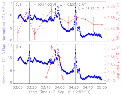
Figure 5: (a) Evolutions of the 171 Å flux (normalized as in Figure 2) and the unsigned vertical electric current $I_{z}$, which is integrated in the field of view as shown in Figure 4. Blue stars mark the normalized 171 Å flux and red diamonds mark the unsigned vertical electric current $I_{z}$. (b) The electric current evolution curves at the first and third peaks have been shifted to the second peak and the total profile is shown with a continuous line. The shifted time differences are $t_{2}-t_{1}$ and $t_{3}-t_{2}$ for the two curves (denoted by dashed and dash-dotted lines), respectively. Note that the vertical axes for both the 171 Å flux and $I_{z}$ do not start from zero.

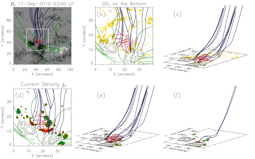
Figure 6: (a) Magnetic field lines computed from the nonlinear force-free field model. Different colors indicate different field line systems. The background is the vertical magnetic field $B_{z}$ shown with grey levels. White/black color represents positive/negative magnetic polarity. The box marks the field of view shown in panels (b)–(f). (b, c) Orange ribbons represent the QSL sections on the photosphere. Only the QSLs with the squashing degree $Q\geq 10^{14}$ are plotted. Grey/black contours are the same as that in Figure 4c. (d, e) Magnetic field lines overlaid on the photospheric distribution of the vertical electric current density $j_{z}$ as shown in Figure 4c. The current $j_{z}$ is computed with the non-preprocessed vector magnetic field. (f) Similar to panels (d) and (e) but only some sample field lines with magnetic dips are shown.

2.5 Magnetic Configuration before the Recurrent Jets

The magnetic configuration is one of the necessary information for discriminating different magnetic reconnection models. For this reason, we study the three-dimensional magnetic field with the nonlinear force-free field (NLFFF) extrapolation of the coronal field from the vector magnetic field as the boundary condition. The optimization method is selected for the NLFFF extrapolation (Wheatland et al., 2000; Wiegelmann, 2004). The bottom boundary is provided by the SDO/HMI vector magnetic field at 03:00 UT, so just before the studied jets. The projection effect has been corrected as described in Section 2.2. Since the photospheric vector magnetic field does not satisfy the force-free condition, we apply the preprocessing method to remove the net magnetic force and torque on the bottom boundary (Wiegelmann et al., 2006). A requirement for the preprocessing is that, the magnetic field at the bottom boundary needs to be isolated and flux balanced. Therefore, we select a field of view as shown by the dotted box in Figure 1d to enclose the major magnetic flux of AR 11106. Since removing the projection effect changes the geometry of the field of view, we cut off the edges where the data are incomplete to get a rectangle box, which is resolved by $932\times 486$ grid points with $\Delta x=\Delta y\approx 0.5^{\prime\prime}$. In order to measure the flux balance quantitatively, we define the flux balance parameter as

$$\epsilon_{f}=\frac{\sum_{i}(B_{z})_{i}\mathrm{d}S}{\sum_{i}|(B_{z})_{i}|\mathrm{d}S},$$ (2)

where the pixel index $i$ runs all over the field of view, and $\mathrm{d}S$ is the area of one pixel. The flux balance parameter $\epsilon_{f}$ is about 0.03 for the magnetic field in this field of view, which is a tolerably small imbalance.

The boundary field of view for the NLFFF extrapolation is shown in Figure 6a. There are two reasons why we use this small field of view. First, the region of interest where the jets originate is small. It is acceptable if we put it in the center. Secondly, the spatial sampling of SDO/HMI is high ($0.5^{\prime\prime}$). Thus, in the selected field of view (about $100^{\prime\prime}\times 100^{\prime\prime}$) and the height range, the computation box includes $200\times 200\times 200$ grid points, which are reasonable sizes for the computation. However, DeRosa et al. (2009) pointed out that it is critical for the vector magnetic field to cover as large areas as possible for successful NLFFF modeling. In order to fulfill this requirement in the limited field of view, we use the following way to prepare the boundary and initial conditions for the higher-resolution NLFFF extrapolation. First, we compute a lower-resolution NLFFF with the vector magnetic field in the field of view used above for the preprocessing as shown by the dotted box in Figure 1d. Due to the limitation of computation resources, the lower-resolution NLFFF is computed in a box of $466\times 243\times 201$ grid points with $\Delta x=\Delta y=\Delta z\approx 1.0^{\prime\prime}$. Then, we cut out a sub-volume in the field of view as shown in Figure 6a with a height of $100^{\prime\prime}$ and interpolate the NLFFF to the spatial resolution of $\Delta x=\Delta y=\Delta z\approx 0.5^{\prime\prime}$. The interpolated NLFFF is used as the initial, lateral, and top boundary conditions for the higher-resolution NLFFF extrapolation. The bottom boundary is provided by the aforementioned preprocessed vector magnetic field in the field of view as shown in Figure 6a, which is cut from the larger flux-balanced area. We use a buffer zone with 25 grid points, in the NLFFF optimization method, to decrease the effect of these boundaries. The weighting function decreases from 1 to 0 with a cosine profile in the buffer zone. Finally, we refer to Wheatland et al. (2000) and Wiegelmann (2004) for more detailed descriptions of the extrapolation method.

We adopt two metrics to test if the NLFFF has reached the force-free and divergence-free state. The force-free metric is defined as the current-weighted average of $\sin\theta$ (Wheatland et al., 2000):

$$<\mathrm{CW}\sin\theta>=\frac{\sum_{i}J_{i}\sin\theta_{i}}{\sum_{i}J_{i}},$$ (3)

where

$$\sin\theta_{i}=\frac{|\mathbf{J}_{i}\times\mathbf{B}_{i}|}{J_{i}B_{i}},$$ (4)

$\theta$ represents the angle between the current density $\mathbf{J}$ and the magnetic field $\mathbf{B}$, and $B=|\mathbf{B}|$, $J=|\mathbf{J}|$. The summation is done in the sub-domain of $77\times 75\times 35$ grid points, whose projection is shown as the solid box in Figure 6a. Only the grid points where $J\geq 0.02$ A m^-2 (the noise level in Section 2.4) are considered in computing $\sin\theta$. For a perfectly force-free magnetic field, the force-free metric should be zero, i.e., the current density $\mathbf{J}$ and the magnetic field $\mathbf{B}$ are parallel to each other. The divergence-free metric is defined as the unsigned average of the fractional flux unbalance, $<|f_{i}|>$, where

$$|f_{i}|=\frac{|(\nabla\cdot\mathbf{B})_{i}|}{6B_{i}/\Delta x}.$$ (5)

The divergence-free metric is computed in the same domain as that for the force-free metric, while the difference is that all the grid points of the sub-domain are considered. This metric should be zero in a truly divergence-free field.

The force-free and divergence-free metrics for the NLFFF model are $0.19$ and $3.0\times 10^{-3}$, respectively. The corresponding angle for the force-free metric, which is defined as $\arcsin<\mathrm{CW}\sin\theta>$, is $11.0^{\circ}$. Metcalf et al. (2008) compared various NLFFF algorithms using simulated chromospheric and photospheric vector fields. The force-free metric $0.19$ that we derive here is slightly better than that of 0.26 using the preprocessed and smoothed photospheric boundary with the optimization code of Wiegelmann (2004). However, it is larger, therefore worse, than the force-free metric 0.11 using the chromospheric boundary. The divergence-free metric $3.0\times 10^{-3}$ is larger (and worse) than both the metrics using the chromospheric and preprocessed and smoothed photospheric boundaries with the optimization method as listed in Table 5 of Metcalf et al. (2008), since they adopted simulated vector magnetic fields as boundary conditions, which are smoother than the observational boundaries that we use in this paper.

Some selected magnetic field lines in the NLFFF model are plotted in Figure 6. The overall magnetic configuration in Figure 6a shows different connectivities with small closed field lines linking the small diverging bipole (represented by the red lines connecting positive polarities p1 and p2 to negative ones n1 and n2) and long field lines (represented by the blue lines anchored in polarities N0 and N1). We find no magnetic null point in between these two set of field lines, so no separatrix. Rather, a continuous but drastic change of magnetic connectivity, so a QSL, is separating both types of connectivities. We compute the squashing degree $Q$ as defined in Titov et al. (2002) to locate the position of the QSLs. Figures 6b and 6c show the QSL sections on the bottom boundary. The closed (red) and long (blue) field lines are clearly separated by QSLs between them.

We also overlay the magnetic field lines on the photospheric distribution of the vertical electric current density $j_{z}$ as shown in Figures 6d and 6e. The footpoints of those field lines close to the QSL are rooted on the regions where $j_{z}$ is large. This result is coherent with previous findings where concentrated electric currents have been found at the border of the QSLs in flare configurations (see Démoulin et al., 1997, and references therein). For a thin QSL, a moderate difference of magnetic stress across the QSL creates strong electric current. Then, a current layer is easily build up at a QSL. For the first time, the high temporal cadence and magnetic sensitivity of SDO/HMI allows to diagnose such current layer evolution for such small events as the studied jets.

Due to the existence of the parasitic positive magnetic polarities, some blue field lines are bent down from higher altitudes to lower altitudes. Magnetic dips and bald patches are present where the magnetic field lines are bent down as shown in Figure 6f. We refer to the following theoretical or observational papers for detailed definition and analysis of magnetic dips and bald patches, such as Titov et al. (1993), Bungey et al. (1996), Mandrini et al. (2002), and Démoulin (2005). However, it is not clear if the bald patches played any role in the magnetic reconnection of the studied jets, which asks for further studies.

3 Discussion and Conclusion

In summary, we find that three EUV jets observed by SDO/AIA from 03:00 to 05:00 UT on 2010 September 17 recurred in the same region close to the border of AR 11106. The time differences between the three successive 171 Å peaks are 40 minutes and 25 minutes. On the border of the following negative polarity, parasitic positive polarities (polarities p1 and p2 in Figure 3) are present close to the footpoints of the EUV jets. They are parts of a magnetic bipole which is growing in size as shown by the diverging flow pattern. The line-of-sight magnetic flux evolution does not have a clear relationship with the 171 Å flux evolution. However, the high time cadence of SDO/HMI (12 minutes for the vector magnetic field) allows us to follow the photospheric current evolution. We integrate the absolute vertical electric current density found in the region of the jets. The peaks of this total current have a good temporal coincidence with the peaks of the 171 Å flux.

The aforementioned features can only be partly explained by the emerging flux model (Shibata et al., 1992b) and the converging flux model (Priest et al., 1994) since the newly emerged magnetic flux is consistent with the former model and the bald patch configuration is consistent with the latter one. But both models are two dimensional with magnetic reconnection in separatrices (as implied by their dimensionality), while the magnetic connectivity is not necessarily discontinuous in the three dimensional space. The above models can be generalized to three dimensional configuration having a magnetic null point (e.g., Moreno-Insertis et al., 2008; Török et al., 2009; Pariat et al., 2009, 2010). However, in the present study, no null point is found in the corona with the NLFFF extrapolation. Rather continuous changes of connectivity are present with drastic changes at some locations. Indeed, the computed coronal configuration has a QSL separating a small-scale evolving double bipole (polarities p1–n1 and p2–n2 in Figure 3) from the large scale AR magnetic field, a configuration comparable to those found previously, e.g. in an X-ray bright point (Mandrini et al., 1996).

The temporal evolution of the photospheric magnetic field (see the movie attached to Figure 3) as well as the velocities deduced by LCT both indicate divergent flows in the small parasitic bipoles. These flows would force the closed field lines of the small parasitic bipole to grow in size, and to interact with the overlaying large scale field lines (Figure 6). Such kind of evolving magnetic configuration is known to build up a narrow current layer in the QSL as conjectured analytically (Démoulin et al., 1996) and found in numerical simulations even for relatively small displacements (Aulanier et al., 2005; Effenberger et al., 2011). The main reason is that the magnetic stress of very distant regions, generated by photospheric flows, are brought close to one another, typically over the QSL thickness. This current layer becomes thinner and stronger with time. When the currents reach the dissipative scale, there is a breakdown of ideal MHD in the QSLs, magnetic reconnection occurs and part of the magnetic energy is released (Aulanier et al., 2006). In the above studied configuration, this process would create some newly formed lower-lying field lines with less shear and some newly formed higher field lines, along which hot collimated plasma are ejected into the higher corona.

The quasi-periodicity and homology of the coronal jets requires two necessary conditions. First, the magnetic energy is injected into the corona uninterruptedly in almost the same region, and secondly, it releases intermittently. The first condition is satisfied by the observed diverging photospheric motions which inject free magnetic energy in the coronal field without changing too much the photospheric magnetic field distribution. The second condition requires the current layer to become thin enough recurrently in order to reconnect and release rapidly part of the plasma trapped in the low lying loops (of the diverging bipole). The observed periodic build up and decrease of the photospheric currents, in phase with the EUV jets (Figure 5), is an evidence that this second condition is met. Indeed, only a small fraction of the current is dissipated, an indication that the reconnection stops rapidly when the current layer weakens. Then, the next build up of current starts from a non-potential configuration. This allows a relatively fast build up of a new thin current layer and may explain the small time interval between the jets (40 and 25 minutes). The photospheric flows displace the magnetic polarities by only about 300–480 km during the successive jets, where we use $v=0.2$ km s^-1 estimated by the LCT velocity data as the average velocity in the encircled region of Figure 3.

What is still surprising is that the build-up and decay times of the currents are comparable (Figure 5). Usually, the build-up time is thought to be much longer than the decay time for many solar activities, such as flares and coronal mass ejections (CMEs). A reason for the comparable time scale could be the limited time cadence of SDO/HMI including the constrain of a large enough signal to noise ratio, so this kind of study needs a higher cadence and better polarimetric accuracy to get a more precise temporal evolution of the currents. We mimic a higher temporal cadence by supposing that the evolution processes are the same, then we combine the current measurements of the three jets using the EUV flux maximum as a time reference. With these limits, we find a current maximum near the beginning of the EUV flux rise, about ten minutes before the EUV flux maximum. This indicates that the free magnetic energy starts to decrease as soon as there is an evidence of reconnection.

In conclusion, we find evidence indicating that the studied recurrent coronal jets are caused by magnetic reconnection in the QSL present between a diverging bipole and the main AR magnetic field. Magnetic energy is injected by the continuous diverging motions observed at the photospheric level. We assume that this process has build a thin current layer whose photospheric cross sections is deduced from the vector magnetograms. The current evolution is found in phase with the EUV flux with a current maximum present before the jets followed by a relaxation to lower value. However, this evolution of the current intensity is limited to around 8% of the average background. Note that only the vertical component of electric currents are derived on the photosphere. If the NLFFF assumption is valid, the coronal currents are directly related to the photospheric currents, since $\alpha=\mu_{0}j_{z}/B_{z}$ and $\alpha$ is constant along a field line. Therefore, we conclude that the magnetic system always stays close to the resistive instability of the current layer. The jets does not change the photospheric vertical current distribution too much and only a moderate photospheric evolution is needed to restart a new jet.

All together, we interpret these observations as the consequence of the continuous photospheric driving of the coronal field. A thin current layer is built in the QSL, where the magnetic field reconnects when the electric currents are strong enough and stops reconnecting soon later on. The magnetic reconnection dissipates only a small part of the electric currents. The above phenomena repeat in time and drive the recurrent jets as the confined plasma in the closed loops is accelerated, after reconnection, into the large scale field.