Model-based dose finding under model uncertainty using general parametric models

Abstract

Statistical methodology for the design and analysis of clinical Phase II dose response studies, with related software implementation, are well developed for the case of a normally distributed, homoscedastic response considered for a single timepoint in parallel group study designs. In practice, however, binary, count, or time-to-event endpoints are often used, typically measured repeatedly over time and sometimes in more complex settings like crossover study designs. In this paper we develop an overarching methodology to perform efficient multiple comparisons and modeling for dose finding, under uncertainty about the dose-response shape, using general parametric models. The framework described here is quite general and covers dose finding using generalized non-linear models, linear and non-linear mixed effects models, Cox proportional hazards (PH) models, etc. In addition to the core framework, we also develop a general purpose methodology to fit dose response data in a computationally and statistically efficient way. Several examples, using a variety of different statistical models, illustrate the breadth of applicability of the results. For the analyses we developed the R add-on package DoseFinding, which provides a convenient interface to the general approach adopted here.

1 Introduction

Finding the right dose is a critical step in pharmaceutical drug development. The problem of selecting the right dose or dose range occurs at almost every stage throughout the process of developing a new drug, such as in microarray studies [25], in-vitro toxicological assays [8], animal carcinogenicity studies [18], Phase I studies to estimate the maximum tolerated dose [26], Phase II studies covering dose ranging and dose-exposure-response modeling [20], Phase III studies for confirmatory dose selection, and post-marketing studies to further explore dose response in specific subgroups defined by region, age, disease severity and other covariates [31, 32, 22]. In recent years, considerable effort has been spent on improving the efficiency of dose finding throughout drug development [37, 12, 24]. Despite these efforts, however, improper dose selection for confirmatory studies, due to lack of sufficient dose response knowledge for both efficacy and safety at the end of Phase II, remains a key driver of the ongoing pipeline problem experienced by the pharmaceutical industry [5, 28].

Statistical analysis methods for late development dose finding studies can be roughly categorized into modelling approaches to characterize the dose response relationship [30, 36] and multiple test procedures for dose response signal detection [34] or confirmatory dose selection [35, 9]. Hybrid approaches combine aspects of multiple testing with modeling techniques to overcome the shortcomings of either approach [38, 10]. More recently, considerable research has focused on extending these methods to response-adaptive designs that offer efficient ways to learn about the dose response through repeated looks at the data during an ongoing study [16, 15, 23, 4].

Most statistical methodology for dose response analysis has been introduced in the context of a normally distributed, homoscedastic endpoint, with a parallel group design, in which each patient receives only one treatment. In practice, however, one often faces more complex study designs (e.g., cross-over designs), where a heteroscedastic or non-normally distributed endpoint is measured (e.g., binary, count and sometimes time-to-event data). One approach is to extend the existing methodology using generalized non-linear models or generalized non-linear mixed effects models. However, these extensions are typically specific to each new situation. In addition general purpose software for these types of models is not available and a case-by-case implementation requires a major coding effort. In this paper, we describe an overarching hybrid approach, combing multiple comparisons and modeling, to the analysis of dose response data for general parametric models and general study designs, that allows for a straightforward computer implementation.

Figure 1: Overview of MCPMod approach

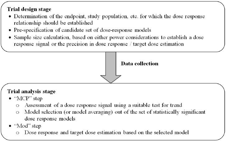
More specifically, we extend the MCPMod approach [10], which was originally introduced for normal, homoscedastic, independent data. This approach provides the flexibility of modeling for dose response and target dose estimation, while accounting for model uncertainty through the use of multiple comparison and model selection/averaging procedures. The approach can be described in two main steps (Fig. 1). At the trial design stage the clinical team needs to decide on the core aspects of the trial design, as in any other trial. Specific for MCPMod is that a candidate set of plausible dose response models is pre-specified at this stage, based on available pharmacokinetic data/dose response information from similar compounds, etc. This gives rise to a set of optimal contrasts used to test for the presence of a dose response signal consistent with the corresponding candidate models. In case of large model uncertainty, this candidate set should be chosen to cover a sufficiently diverse set of plausible dose response shapes

The trial analysis stage consists of two main steps: The MCP and the Mod steps. The MCP step focuses on establishing evidence of a drug effect across the doses, i.e., detecting a statistically significant dose response signal for the clinical endpoint and patient population investigated in the study. This step will typically be performed using an efficient test for trend, adjusting for the fact that multiple candidate dose response models are being considered. If a statistically significant dose response signal is established, one proceeds with determining a reference set of significant dose response models by discarding the non-significant models from the initial candidate set. Out of this reference set, a best model is selected for dose estimation in the last stage of the procedure, using existing non-linear regression methods [2]. The selected dose-response model is then employed to estimate target doses using inverse regression techniques and possibly incorporating information on clinically relevant effects. The precision of the estimated doses can be assessed using, for example, bootstrap methods.

The original MCPMod method proposed by [10] was intended to be used with parallel group designs with a normally distributed, homocedastic response. Although that covers a good range of dose finding designs utilized in practice, the restrictions of the original method create serious practical limitations to its wider use in drug development. For example, binary, count, and time-to-event endpoints, though frequently used in many disease indications, are not covered by the original MCPMod formulation. Likewise, longitudinal patient data, like in crossover studies, with its implicit within-patient correlation, cannot be properly analyzed with the original formulation of the MCPMod methodology. In what follows, we extend the MCPMod methodology, to perform dose response modeling and testing in the context of general parametric models and for general study designs, in a similar way as [19] extended certain simultaneous inference procedures. Note that, even though we focus on extending the MCPMod approach, the results of this paper remain valid, in particular, if only a multiple comparison or a modeling approach is to be applied.

We introduce the proposed extension in Section 2. In Section 3 we describe an efficient approach for dose response model fitting, which is evaluated in terms of asymptotic considerations and simulations. In Section 4 we use several case studies to illustrate the proposed methodology and its implementation with the R add-on package DoseFinding [6]. In summary the method is illustrated for binary, overdispersed count, time-to-event data (based on the Cox PH model) and longitudinal data with patient specific random effects.

2 Generalized MCPMod

This section describes an extension of the original MCPMod approach that can be used whenever the response variable can be described by a parametric model in which one of the parameters captures the dose response relationship. We show how the basic ideas and concepts of the original MCPMod can be extended to this setting.

2.1 Basic concepts, notation and assumptions

In the original description of MCPMod, the expected value of the response is utilized as the parameter capturing the dose response relationship. The key idea of the extended version of MCPMod is to decouple the dose response model from the expected response, focusing, instead, on a more general characterization of dose response via some appropriate parameter in the probability distribution of the response. To be more concrete, let ${{\boldsymbol{y}}}$ denote the response vector of an experimental unit in the trial (e.g., a patient) which has been assigned a dose $x$. The following results can easily be extended to the case of multiple doses ${{\boldsymbol{x}}}$, if needed. We assume that ${{\boldsymbol{y}}}$ follows the distribution function given by

$${{\boldsymbol{y}}}\sim F\left({{\boldsymbol{z}}},{\boldsymbol{\eta}},\mu(x)\right),$$ (1)

where $\mu(x)$ denotes the dose response parameter, ${\boldsymbol{\eta}}$ the vector of nuisance parameters, and ${{\boldsymbol{z}}}$ the vector of possible covariates. The key features of extended version of MCPMod can then be formulated with respect to $\mu(x)$, such as:

• accounting for uncertainty in the dose response model via a set of candidate dose response models,

• testing of dose response signal via contrasts based on dose response shapes,

• model selection via information criteria, or model averaging to combine different models, and

• dose response estimation and dose selection via modeling.

Because all dose response information is assumed to be captured by $\mu(x)$, the interpretability of this parameter is critical for communicating with clinical teams, choosing candidate dose response shapes, specifying clinically relevant effects for target dose estimation, etc. To better illustrate this point, consider a time-to-event endpoint that is assumed to follow a Weibull distribution. The Weibull distribution is typically parameterized by a scale parameter $\lambda$ and shape parameter $\alpha$, neither of which has an easy clinical interpretation. For the purpose of MCPMod modelling the model could be reparameterized in terms of the median time to event $\mu=\left[\log(2)\right]^{1/\alpha}/\lambda$ and $\alpha$, and then one would use $\mu(x)$ as an interpretable dose response parameter.

All dose response models of interest in this paper can be expressed as

$$f(x,{\boldsymbol{\theta}})=\theta_{0}+\theta_{1}f^{0}(x,{\boldsymbol{\theta}}^{0}),$$ (2)

where $f^{0}$ denotes the so-called standardized model function and ${\boldsymbol{\theta}}^{0}$ its parameter vector. For example, for $f^{0}(x,\theta^{0})=x$ one obtains the linear model $f(x,{\boldsymbol{\theta}})=\theta_{0}+\theta_{1}x$ and for $f^{0}(x,\theta^{0})=x/(x+\theta^{0})$ the Emax dose response model $f(x,{\boldsymbol{\theta}})=\theta_{0}+\theta_{1}x/(x+\theta^{0})$; see  [10, 7] for more examples. Dose response models of the form (2) are specified as candidate models for $\mu(x)$. Covariates may also be included in (2), at the model fitting stage, but we leave them out for now to keep the notation simple.

Assume that $K$ distinct doses $x_{1},\ldots,x_{K}$ are utilized in a trial, with $x_{1}$ denoting placebo. Assume further that $M$ candidate models $f_{1},\ldots,f_{M}$ have been chosen to capture the model uncertainty about $\mu(x)$. We define the dose response parameter vector associated to candidate model $m$ as ${\boldsymbol{\mu}}_{m}=\left(\mu_{m,1},\ldots,\mu_{m,K}\right),$ where $\mu_{m,i}=f_{m}(x_{i},{\boldsymbol{\theta}}),i=1,\ldots,K,m=1,\ldots,M$.

For the purpose of obtaining estimates of the dose response, we initially consider an analysis-of-variance (ANOVA) parametrization for the dose response parameter $\mu(x_{i})=\mu_{i},\;i=1,\ldots,K$. That is, we allow a separate parameter $\mu_{i}$ to represent the dose response at each dose level. Let $\widehat{{\boldsymbol{\mu}}}$ denote the vector of estimated dose response parameters under the ANOVA parametrization, obtained using the appropriate estimation method for the general parametric model (1) via maximum likelihood (ML), generalized estimating equations (GEE), partial likelihood, etc. Note that these type of ANOVA estimates are easily available from standard statistical software packages. The key assumption underpinning the extended version of MCPMod is that $\widehat{{\boldsymbol{\mu}}}$ has an approximate distribution ${\cal N}\left({\boldsymbol{\mu}},{{\boldsymbol{S}}}\right),$ where ${{\boldsymbol{S}}}$ denotes the variance-covariance of $\widehat{{\boldsymbol{\mu}}}$. This assumption can be shown to hold for most parametric estimation problems, such as, generalized linear models, parametric time-to-event models, mixed-effects models, GEE, etc. Note that ${{\boldsymbol{S}}}$ is a function of $n$ and converges to $\mathbf{0}$ as $n\rightarrow\infty$. Furthermore, ${\boldsymbol{S}}$ may or may not depend on ${\boldsymbol{x}}$. For example, dependence on ${\boldsymbol{x}}$ arises if unequal variances for different dose levels $x_{i}$ are considered. The estimation of ${\boldsymbol{\theta}}$ is done in a separate second stage based on $\widehat{{\boldsymbol{\mu}}}$ and an estimate $\widehat{{\boldsymbol{S}}}$ of its covariance matrix. Section 3 explains this in detail.

2.2 Implementation of the MCP step

The MCP step consists of specifying a set of candidate models for the dose response relationship $\mu(x)$. To that end, one needs to specify families of candidate models (e.g., linear, Emax, logistic, quadratic). In addition, to derive optimal model contrasts, one needs to determine guesstimates for the non-linear parameters ${\boldsymbol{\theta}}^{0}$, such as the ED₅₀ parameter for the Emax model. Note that the shape of the dose response model function is determined by the parameter ${\boldsymbol{\theta}}^{0}$, which is why only guesstimates for this parameter are needed to derive optimal model contrasts. As mentioned earlier, the clinical interpretability of $\mu(x)$ is critical for this step. Further details on and strategies for the specification of candidate models and corresponding guesstimates are given in [29].

Given these guesstimates, each candidate model shape determines an optimal contrast for a trend test to evaluate the associated dose response model signal, such as a linear trend or a trend based on an Emax model with ED${}_{50}=2$. The optimal contrasts are applied to the previously described ANOVA estimates $\widehat{{\boldsymbol{\mu}}}$, with the associated asymptotic distribution used for implementing the corresponding tests (i.e., critical values and p-values). It can be shown that the (optimal) contrast for testing the hypothesis of a flat dose-response profile with maximal power for a single candidate model shape ${\boldsymbol{\mu}}_{m}$ is given by

$${{\boldsymbol{c}}}^{opt}\propto{{\boldsymbol{S}}}^{-1}\left({\boldsymbol{\mu}}^{0}_{m}-\frac{{\boldsymbol{\mu}}^{0\prime}_{m}{{\boldsymbol{S}}}^{-1}{{\boldsymbol{1}}}}{{{\boldsymbol{1}}}^{\prime}{{\boldsymbol{S}}}^{-1}{{\boldsymbol{1}}}}\right),$$ (3)

where ${\boldsymbol{\mu}}^{0}_{m}=(f^{0}_{m}(x_{1},{\boldsymbol{\theta}}^{0}),\ldots,f^{0}_{m}(x_{K},{\boldsymbol{\theta}}^{0}))^{\prime}$ and ${\boldsymbol{\theta}}^{0}$ is the parameter for which guesstimates are required, see [10] and Appendix A. For convenience, we normalize the contrast coefficients such that $||{{\boldsymbol{c}}}_{opt}||=1$.

The implementation of contrast tests for the candidate models is done similarly to the original MCPMod approach. Let ${{\boldsymbol{c}}}_{1}^{opt},\ldots,{{\boldsymbol{c}}}_{M}^{opt}$ represent the optimal contrasts corresponding to the set of candidate models and ${{\boldsymbol{C}}}^{opt}=\left[{{\boldsymbol{c}}}_{1}^{opt}\cdots{{\boldsymbol{c}}}_{M}^{opt}\right]$ the associated optimal contrast matrix. The contrast estimates are then given by $\left({{\boldsymbol{C}}}^{opt}\right)^{\prime}\widehat{{\boldsymbol{\mu}}}$, being asymptotically normally distributed with mean $\left({{\boldsymbol{C}}}^{opt}\right)^{\prime}{\boldsymbol{\mu}}$ and covariance matrix $\left({{\boldsymbol{C}}}^{opt}\right)^{\prime}{{\boldsymbol{S}}}{{\boldsymbol{C}}}^{opt}.$ It follows that the asymptotic z-test statistic for the m^th candidate model hypotheses $H_{0}:\left({{\boldsymbol{c}}}_{m}^{opt}\right)^{\prime}{\boldsymbol{\mu}}=0$ vs. $H_{0}:\left({{\boldsymbol{c}}}_{m}^{opt}\right)^{\prime}{\boldsymbol{\mu}}>0$ is given by $z_{m}=\left({{\boldsymbol{c}}}_{m}^{opt}\right)^{\prime}\widehat{{\boldsymbol{\mu}}}/\left[\left({{\boldsymbol{C}}}^{opt}\right)^{\prime}{{\boldsymbol{S}}}{{\boldsymbol{C}}}^{opt}\right]_{m,m}^{1/2},$ with $[{{\boldsymbol{A}}}]_{m,m}$ denoting the m^th diagonal element of the matrix ${{\boldsymbol{A}}}$. The test statistic used for establishing an overall dose response signal is the maximum $z_{(M)}=\max_{m}z_{m}$ of the individual model test statistics. Critical values for tests with (asymptotically) exact level $\alpha$ can be derived from the joint distribution of ${{\boldsymbol{z}}}=\left(z_{1},\ldots,z_{M}\right)$, which is easily obtained from the joint distribution of the contrast estimates given previously, and using

$$P(z_{(M)}>q)=1-P(z_{(M)}\leq q)=1-P({{\boldsymbol{z}}}\leq q{{\boldsymbol{1}}}).$$ (4)

Multiplicity adjusted p-values for the individual model contrast tests can be derived similarly. The mvtnorm package in R includes functions to calculate quantiles and probabilities for the underlying multivariate normal distributions [17].

If the optimal contrasts and the critical values also depend on ${{\boldsymbol{S}}}$, one needs guesstimates for nuisance parameters appearing in the covariance matrix at the planning stage, as well. This is a difference compared to the normal homoscedastic setting without covariates, where ${{\boldsymbol{S}}}$ is proportional to a diagonal matrix with the the reciprocal of the group sample sizes on the diagonal. Once data becomes available, the z-statistics for the model contrast tests are calculated and their maximum used for the dose response test. At this stage, one can obtain the estimated $\widehat{{{\boldsymbol{S}}}}$ matrix from the observed data, and use this to recalculate optimal contrasts and the critical value for the test. Note that the guesstimates for the parameters ${\boldsymbol{\theta}}^{0}$ are not recalculated based on the observed data, as this would lead to a serious Type I error rate inflation. For the purpose of the multiple contrast test, the guesstimates pre-specified at the planning stage for ${\boldsymbol{\theta}}^{0}$ should be used.

2.3 Implementation of the Mod step

Once a dose response signal is established, one proceeds to the Mod step, fitting the dose response profile and estimating target doses based on the models identified in the MCP step. There are many ways to fit the dose response models to the observed data, including approaches based on maximizing the likelihood (ML) or the restricted likelihood. However, a direct ML approach requires the derivation of the likelihood in every specific case, with a considerable amount of model-specific coding involved. We therefore suggest an alternative two-stage approach to dose response model fitting that utilizes generalized least squares. This approach is described in more detail in Section 3. It relies on asymptotic results, but has the appeal of being of general purpose application, as it depends only on $\widehat{{\boldsymbol{\mu}}}$ and $\widehat{{{\boldsymbol{S}}}}$. In addition, as shown later in the simulation study, its finite and large sample properties are similar to those of the approaches based on the full likelihood.

Model selection can be based on the maximum z-statistics, or using information criteria, such as the AIC or the BIC. Estimates of the latter under the model fitting approach are discussed in the next section. Estimation of target doses is done based on the selected fitted model for the dose response parameter [7].

Alternatively, model averaging approaches can be used to avoid the need to select a single model. The individual AIC and BIC values for the candidate models with significant contrast test statistics determine the model averaging weights [11]. This applies both to dose response and target dose estimation.

The generalization of MCPMod described in this section has focused on testing and estimation associated with the full dose response profile, that is, including the response at placebo and the entire dose range utilized in the study. In practice, there are cases in which inference might focus on the placebo-adjusted dose response (or more generally a control-adjusted response), that is, the dose response with the placebo or control effect subtracted $f_{C}(x,{\boldsymbol{\theta}})=f(x,{\boldsymbol{\theta}})-f(0,{\boldsymbol{\theta}})$. This could become relevant, for example, if covariates are added to the placebo response $\theta_{0}$ in (2). In the context of time-to-event data, the focus on placebo-adjusted dose response will occur naturally when modeling the hazard ratio as a function of dose. As shown in Appendix B, all results presented in this section, including the derivation of optimal contrasts, as well as the model fitting results described in the next section, apply equally in the context of placebo-adjusted dose response.

3 Non-linear dose response model fitting using a two-stage, generalized least squares approach

In this section we describe an efficient methodology for fitting nonlinear dose response models that can be used for the Mod step of the MCPMod methodology. The fitting is done in two stages: First, the ANOVA estimates $\widehat{{\boldsymbol{\mu}}}$ and $\widehat{{\boldsymbol{S}}}$ introduced in Section 2 are obtained. Second, the parameter ${\boldsymbol{\theta}}$ is estimated by fitting the dose response model to the ANOVA estimates from the first step using a generalized least squares estimation criterion. In Section 3.1, we establish consistency and asymptotic normality of this estimate. In Section 3.2 we assess the accuracy of the asymptotic results via a simulation study.

3.1 Asymptotic results

Assume that we have dose response estimates $\widehat{{\boldsymbol{\mu}}}=(\widehat{\mu}_{1},\ldots,\widehat{\mu}_{K})^{\prime}$ obtained from an ANOVA-type parameterization of ${\boldsymbol{\mu}}$ which allows for unrelated mean responses at each of the $K$ dose levels; see Section 2.1. These estimates are assumed to be asymptotically multivariate normal distributed with a covariance matrix consistently estimated by $\widehat{{\boldsymbol{S}}}$. The estimates $\widehat{{\boldsymbol{\mu}}}$ and $\widehat{{\boldsymbol{S}}}$ are easily available from standard statistical packages, see Section 4 for examples using R. Next, we fit the non-linear dose response model $f(x,{\boldsymbol{\theta}})$ to the estimates $\widehat{{\boldsymbol{\mu}}}$ by minimizing the generalized least squares criterion

$$\widehat{{\boldsymbol{\Psi}}}({\boldsymbol{\theta}})=(\widehat{{\boldsymbol{\mu}}}-{\boldsymbol{f}}({\boldsymbol{x}},{\boldsymbol{\theta}}))^{\prime}{{\boldsymbol{A}}_{n}}(\widehat{{\boldsymbol{\mu}}}-{\boldsymbol{f}}({\boldsymbol{x}},{\boldsymbol{\theta}}))$$ (5)

with respect to ${\boldsymbol{\theta}}$ to obtain the estimates $\widehat{{\boldsymbol{\theta}}}$. In Equation (5) we have ${\boldsymbol{f}}({\boldsymbol{x}},{\boldsymbol{\theta}})=(f(x_{1},{\boldsymbol{\theta}}),\ldots,f(x_{K},{\boldsymbol{\theta}}))^{\prime}$ and ${\boldsymbol{A}}_{n}$ denotes a symmetric positive definite matrix. We assume that ${\boldsymbol{A}}_{n}\overset{P}{\rightarrow}{\boldsymbol{A}}$, where $\overset{P}{\rightarrow}$ denotes convergence in probability. In practice we will always use ${\boldsymbol{A}}_{n}=\widehat{{\boldsymbol{S}}}^{-1}$, but this would unnecessarily restrict the discussion at this stage.

Let ${\boldsymbol{\theta}}_{0}$ denote the true value of the parameter ${\boldsymbol{\theta}}$. In Appendix C we show that, under mild regularity conditions, $\widehat{{\boldsymbol{\theta}}}$ is a consistent estimator of ${\boldsymbol{\theta}}_{0}$, i.e., $\widehat{{\boldsymbol{\theta}}}\overset{P}{\rightarrow}{\boldsymbol{\theta}}_{0}$. Furthermore, we have the asymptotic multivariate normality

$$\sqrt{a_{n}}(\widehat{{\boldsymbol{\theta}}}-{\boldsymbol{\theta}}_{0})\overset{d}{\rightarrow}N({\boldsymbol{0}},{\boldsymbol{B}}({\boldsymbol{\theta}}_{0})^{\prime}{\boldsymbol{M}}({\boldsymbol{\theta}}_{0}){\boldsymbol{B}}({\boldsymbol{\theta}}_{0})),$$ (6)

where ${\boldsymbol{M}}({\boldsymbol{\theta}})=a_{n}{\boldsymbol{F}}({\boldsymbol{\theta}})^{\prime}{\boldsymbol{A}}{\boldsymbol{S}}{\boldsymbol{A}}{\boldsymbol{F}}({\boldsymbol{\theta}})$ and ${\boldsymbol{B}}({\boldsymbol{\theta}})=({\boldsymbol{F}}({\boldsymbol{\theta}})^{\prime}{\boldsymbol{A}}{\boldsymbol{F}}({\boldsymbol{\theta}}))^{-1}$, ${\boldsymbol{F}}({\boldsymbol{\theta}})$ denotes the $d\times k$ matrix of partial derivatives $\frac{df(x_{i},{\boldsymbol{\theta}})}{d\theta_{h}}$ ($i=1,...,k$,$\quad h=1,...,d$), $a_{n}$ a non-decreasing sequence of values increasing to infinity as the sample size $n$ goes to infinity.

Selecting ${\boldsymbol{A}}_{n}={\boldsymbol{S}}^{-1}$ would be the best choice, if ${\boldsymbol{S}}$ were known. Provided that $a_{n}{\boldsymbol{S}}\overset{P}{\rightarrow}{\boldsymbol{\Sigma}}$ as $n\rightarrow\infty$, the previous formulas in this case simplify to $\sqrt{a_{n}}(\widehat{{\boldsymbol{\theta}}}-{\boldsymbol{\theta}}_{0})\overset{d}{\rightarrow}N({\boldsymbol{0}},({\boldsymbol{F}}({\boldsymbol{\theta}}_{0}){{\boldsymbol{\Sigma}}}^{-1}{\boldsymbol{F}}({\boldsymbol{\theta}}_{0})^{\prime})^{-1})$ with $\widehat{{\boldsymbol{\theta}}}$ minimizing

$$\widehat{{\boldsymbol{\Psi}}}({\boldsymbol{\theta}})=(\widehat{{\boldsymbol{\mu}}}-{\boldsymbol{f}}({\boldsymbol{x}},{\boldsymbol{\theta}}))^{\prime}{{\boldsymbol{S}}}^{-1}(\widehat{{\boldsymbol{\mu}}}-{\boldsymbol{f}}({\boldsymbol{x}},{\boldsymbol{\theta}}))$$ (7)

with respect to ${\boldsymbol{\theta}}$. Because ${\boldsymbol{S}}$ is not known, we will typically use a consistent estimate $\widehat{{\boldsymbol{S}}}$ of it in (7). If the assumptions about the covariance matrix are wrong in the sense that $a_{n}\widehat{{\boldsymbol{S}}}$ does not converge to ${\boldsymbol{\Sigma}}$, then $\widehat{{\boldsymbol{\theta}}}$ will still be consistent and have the asymptotic normal distribution given in (6). In this regard, the suggested estimator is similar to Huber’s robust estimator ([21]; Section 4.6 in [13]), but this aspect will not be further utilized.

Note that this two-stage, generalized least squares estimate is quite similar to the ML estimate: For normal homoscedastic data both approaches lead to exactly the same estimate, while, for example, in generalized linear model settings the two estimators have the same large-sample variance; see Chapter 4.3 in [14].

The computational advantage of using this two-stage approach is that the target function in (7) that is optimized numerically is low-dimensional: The dimension is equal to the number of different dose levels and the target function can thus be evaluated quite efficiently, while the target function in a full likelihood approach depends on the complete data set. This difference in speed becomes relevant in clinical trial settings, as often extensive clinical trial simulations are used to evaluate proposed study designs. Another advantage of the proposed method is its broad applicability to general parametric models.

Model selection criteria are generally defined as $-2\log(L)+\dim({\boldsymbol{\theta}})\tau$, where $L$ denotes the likelihood function evaluated at the maximum likelihood estimate and $\tau$ a penalty for the number of parameters, which depends on the model selection criterion. One approach to model selection is hence to use $\widehat{{\boldsymbol{\Psi}}}(\widehat{{\boldsymbol{\theta}}})+\dim({\boldsymbol{\theta}})\tau$ to compare different dose response models fitted based on the same $\widehat{{\boldsymbol{\mu}}}$ and ${\boldsymbol{S}}$. This criterion is motivated by the fact that, for normally distributed homoscedastic data without covariates, these two approaches are equivalent in terms of selecting the same model: The likelihood function can be split into the sum of the deviation between the observed data and $\widehat{{\boldsymbol{\mu}}}$ and the deviation between $\widehat{{\boldsymbol{\mu}}}$ and ${\boldsymbol{f}}({\boldsymbol{x}},\widehat{{\boldsymbol{\theta}}})$. The deviation of the individual data and $\widehat{{\boldsymbol{\mu}}}$ is identical across the different dose response models, so that the criterion only varies with the deviation between $\widehat{{\boldsymbol{\mu}}}$ and ${\boldsymbol{f}}({\boldsymbol{x}},\widehat{{\boldsymbol{\theta}}})$, which, in case of normal data, is equal to $\widehat{{\boldsymbol{\Psi}}}(\widehat{{\boldsymbol{\theta}}})$. In situations beyond the normal case both approaches might lead to slightly different results, however as (7) is roughly proportional to $-2\cdot$log-likelihood of the ML estimate of ${\boldsymbol{\theta}}$, when discarding the contribution of the first stage ANOVA-type fit (which is equal for all dose response models considered) typically both approaches will lead to very similar results. Subsequently $\tau=2$ will be used and we refer to this criterion as gAIC.

In the next subsection we investigate the properties of the proposed asymptotic approximations via simulations before illustrating it with several applications in Section 4.

3.2 Simulations

In this section we evaluate the asymptotic performance of the approximations provided in Section 3.1 for fitting a single nonlinear dose response model. More specifically, we compare the proposed methods with more traditional maximum likelihood estimation by evaluating the dose response estimation accuracy using simulations. In addition we assess the coverage probability of the resulting confidence intervals for the model parameter ${\boldsymbol{\theta}}$.

3.2.1 Design of simulation study

Throughout the simulations we assume five active dose levels 0.05, 0.2, 0.5, 0.8, 1 plus placebo. We investigate equal group sample sizes of 15, 30, 50, 100, 300 and 1000 patients for each dose. The lower range of the investigated sample sizes is realistic for typical Phase II dose response studies, while the sample sizes of 300 and 1000 are included to assess the asymptotic behavior.

Figure 2: Dose Response Models used for simulation

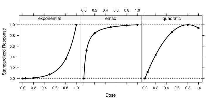
We investigate three types of data: binary data, overdispersed count data using a negative binomial model and time-to-event data using a Cox PH model for estimation. Regarding dose response models, we will utilize an Emax model $\mu(x,\theta)=\theta_{0}+\theta_{1}x/(\theta_{2}+x)$, a quadratic model $\mu(x,\theta)=\theta_{0}+\theta_{1}x+\theta_{2}x^{2}$ and an exponential model $\mu(x,\theta)=\theta_{0}+\theta_{1}(\exp(x/\theta_{2})-1)$. In the simulations, we set $\theta_{2}=0.05$ for the Emax model, $\theta_{2}=0.2$ for the exponential model and $\theta_{1}/\theta_{2}=-5/8$ for the quadratic model; see Figure 2 for the underlying model shapes. The remaining parameters $\theta_{0}$ and $\theta_{1}$ are chosen such that the power for testing the dose with the maximum treatment effect against placebo at the 5% one-sided significance level is 80% for 30 patients per group. This ensures a realistic range of sample sizes (in terms of the signal to noise ratio) is investigated in the simulations.

Data type	Quadratic	Emax	Exponential
binary	$(-1.734,4.335,-2.7094)$	$(-1.734,1.8207,0.05)$	$(-1.734,0.01176,0.2)$
count	$(2,-2,1.25)$	$(2,-0.84,0.05)$	$(2,-0.005427,0.2)$
time-to-event	$(0,-1.8876,1.1797)$	$(0,-0.7928,0.05)$	$(0,-0.005122,0.2)$
normal	$(0,2.61,1.633)$	$(0,1.097,0.05)$	$(0,0.007089,0.2)$

Table 1: Dose Response Model Parameters $(\theta_{0},\theta_{1},\theta_{2})$ used for simulation

Table 1 summarizes the three dose response model specifications for each data type. For binary data, Table 1 gives the the mean on the logit scale. For count data, the logarithm of the mean is as specified in Table 1 and the overdispersion parameter is 1. For time-to-event data, we use an exponential distribution for data generation with the log-means specified in Table 1 and where observations larger than 10 are censored. The mean in the placebo group is 1, so that the log-mean is equal to the difference in log-hazard rates. The Cox PH model is formulated relative to the control group, so that, in this case, the placebo parameter is set to 0 when estimating the dose response model. In addition, we include normally distributed data with $\sigma=1$ as a benchmark comparison, since in this case the two-stage, generalized least squares (GLS) and ML estimates coincide.

We use the two-stage approach from Section 2 to obtain (i) an ANOVA-type model fit to the data by using either a generalized linear model (binary and count data) or a Cox PH model (time-to-event data) with “dose” treated as a factor and (ii) a dose response model fit to the resulting dose response estimates obtained via generalized least squares (7), together with the asymptotic results from Section 3.1. In the simulations, we compare this approach to nonlinear maximum likelihood (binary and count data) and maximum partial likelihood (time-to-event data) estimation using the same link functions as above. For the model fitting step, we assume lower and upper bounds for the $\theta_{2}$ parameter of 0.001 and 5 for the Emax and 0.05 and 5 for the exponential dose response model.

In addition, we assess the coverage probability for three different methods of constructing confidence intervals for the dose response model parameter ${\boldsymbol{\theta}}$. First, we use the generalized least squares (7) together with the asymptotic results from Section 3.1 (denoted below as GLS). Second, we use parametric bootstrap confidence intervals by sampling from the multivariate normal distribution underlying the first stage ANOVA-type estimates and then fitting the nonlinear model to each of these samples using the GLS criterion from (7). The bootstrap confidence intervals are then calculated by taking the 5% and 95% quantiles of the observed sample. For each simulation we used 500 bootstrap samples (denoted below as GLS-B). Finally, we use the maximum likelihood fits and calculate confidence intervals based on the inverse of the Hessian matrix and the usual asymptotic normality assumptions (denoted below as ML).

3.2.2 Results of simulation study

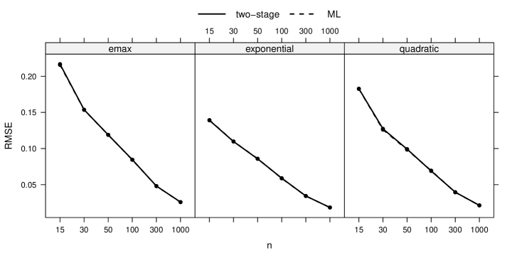
Simulations were run with 2000 replications, using the DoseFinding package version 0.9-1. To illustrate the performance of the GLS and ML methods with regard to dose response estimation, we calculated the root mean squared estimation error averaged over the available doses $\sqrt{\frac{1}{6}\underset{x\in\mathcal{D}}{\sum}(f(x,\widehat{{\boldsymbol{\theta}}})-f(x,{\boldsymbol{\theta}}))^{2}}$, where $\mathcal{D}=\{0,0.05,0.2,0.6,0.8,1\}$. Figures 9, 10 and 11 in the Appendix display the results. It is evident from these plots that both approaches can hardly be distinguished in terms of the mean squared error, indicating that, in terms of dose response estimation, both methods perform almost identically, even for small sample sizes.

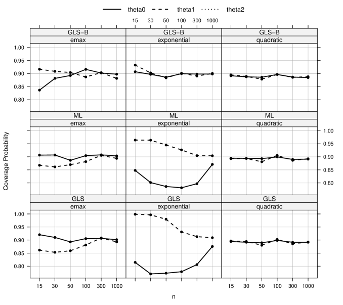
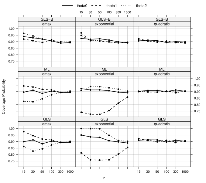
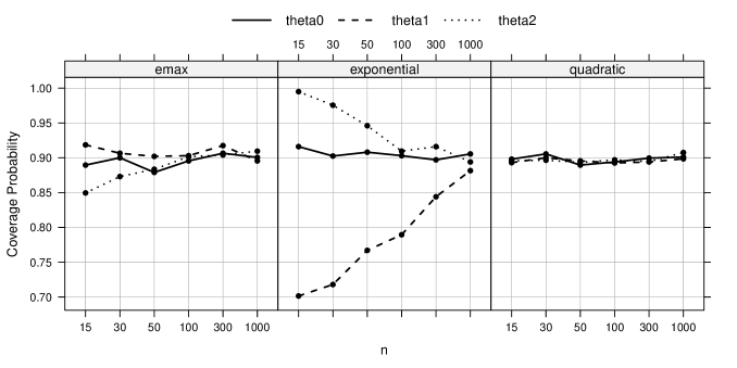
Next, we assess the coverage probability for the three different methods described at the end of Section 3.2.1. Figure 3 displays the results only for the count data case, because the results for the binary and time-to-event data are nearly indentical. We observe that the asymptotic confidence intervals for the GLS and ML methods perform very similarly for all three models under investigation (Emax, exponential, quadratic). Both methods achieve the nominal 90% coverage probability fairly well for the quadratic model, even for small sample sizes. For the Emax model, the nominal coverage probability is achieved at roughly 50-100 patients per group, whereas for the exponential model the coverage probability is achieved only at very large sample sizes (the poor performance of standard asymptotic confidence intervals for nonlinear regression models even for moderate sample sizes is well-known, see for example, [27]). The reason for the better performance under the quadratic model is the fact that it is linear in the model parameters. One reason for why the confidence intervals perform worse for the exponential model than for the Emax model might be that the dose design used in the simulations allows an easier identification of the model parameters under the Emax model, because there are more dose levels in the lower part of the dose range than the upper part.

In contrast, the parametric bootstrap approach GLS-B achieves the 90% nominal coverage probability fairly well for all three dose response models, even at sample sizes as small as 30 patients per group. The GLS-B method thus performs always at least as well as the GLS and ML methods, and the general recommendation is to use this in case of small sample sizes. The approach is computationally more expensive, as it requires repeated fitting of the dose response models, but the bootstrap-based on the GLS two-stage fitting is computionally much more efficient than a traditional bootstrap approach based on ML: The GLS two-stage approach only depends on the ANOVA type estimates and not the individual observations, which makes evaluation of $\widehat{{\boldsymbol{\Psi}}}(\widehat{{\boldsymbol{\theta}}})$ computationally much cheaper than evaluation of the full likelihood function.

Figure 3: Empirical coverage probability (based on 2000 simulations), of 90% confidence intervals.

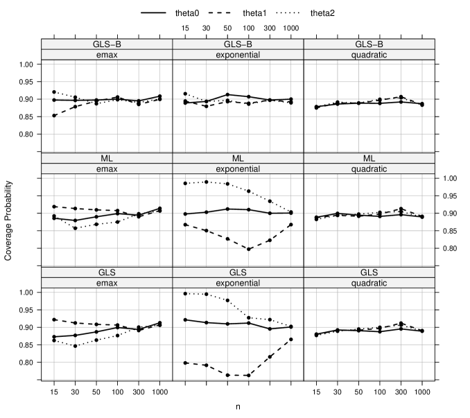
In summary, we conclude that both the GLS and ML methods perform similarly under the different dose response shapes, sample sizes, and data types investigated in the simulation study. This conclusion holds both for the coverage probabilities, as well as for the average estimation error. As mentioned previously, however, the GLS method is very general and computationally more efficient, which facilitates the usage of computationally expensive techniques such as the bootstrap approach.

4 Applications

4.1 Longitudinal modeling of neurodegenerative disease

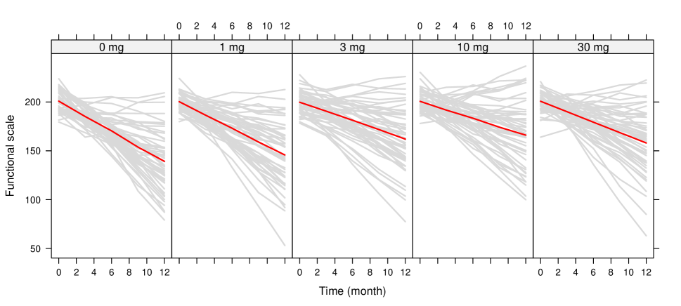
This example refers to a Phase 2 clinical study of a new drug for a neurodegenerative disease. The state of the disease is measured through a functional scale, with smaller values corresponding to more severe neurodeterioration. The goal of the drug is to reduce the rate of disease progression, which is measured by the linear slope of the functional scale over time.

The trial design includes placebo and four doses: 1, 3, 10, and 30 mg, with balanced allocation of $50$ patients per arm. Patients are followed up for one year, with measurements of the functional scale being taken at baseline and every three months thereafter. The study goals are to (i) test the dose-response signal, (ii) estimate the dose-response and (iii) select a dose to be brought into the confirmatory stage of the development program.

The functional scale response is assumed to be normally distributed and, based on historical data, it is believed that the longitudinal progression of the functional scale over the one year of follow up can be modeled by a simple linear trend. We use this example to illustrate the application of MCPMod in the context of mixed-effects models.

We consider a mixed-effects model representation for the functional scale measurement $y_{ij}$ on patient $i$ at time $t_{ij}$:

$$y_{ij}=\left(\beta_{0}+b_{0i}\right)+\left(\mu(x_{i})+b_{1i}\right)t_{ij}+\epsilon_{ij},\;\left[b_{0i},b_{1i}\right]^{\prime}{\sim}N\left({{\boldsymbol{0}}},{\boldsymbol{\Lambda}}\right)\;\mathrm{and}\;\epsilon_{ij}{\sim}N\left(0,\sigma^{2}\right),\mathrm{all\;stoch.\;independent}.$$ (8)

The DR parameter in this case is the linear slope of disease progression $\mu(x)$. If $\mu(x)$ is represented by a linear function of dose $x$, the model in (8) is a linear mixed-effects (LME) model, else it becomes a nonlinear mixed-effects (NLME) model. In particular, under the ANOVA parametrization discussed in Section 2.1, $\mu(x_{i})=\mu_{i}$, (8) is an LME model with different slopes for each dose.

The research interest in this study focuses on the treatment effect on the linear progression slope. At $t=1$ year this is numerically equal to the average change from baseline, and thus easily interpretable. At the planning stage of the trial, the following assumptions were agreed with the clinical team for the purpose of design:

• Natural disease progression slope = -5 points per year.

• Placebo effect = 0 (i.e., no change in natural progression).

• Maximum improvement over placebo within dose range = 2 points increase in slope over placebo.

• Target (clinically meaningful) effect = 1.4 points increase in slope over placebo.

Guesstimates for the variance-covariance parameters were obtained from historical data: $\mathrm{var}\left(b_{0i}\right)=100$, $\mathrm{var}\left(b_{1i}\right)=9$ $\mathrm{corr}\left(b_{0i},b_{1i}\right)=-0.5$, and $\mathrm{var}\left(\epsilon_{ij}\right)=9$. Under these assumptions, it is easy to see that the covariance matrix of the ANOVA-type estimate $\widehat{{\boldsymbol{\mu}}}$ of the slopes ${\boldsymbol{\mu}}=\left(\mu_{1mg},\mu_{3mg},\mu_{10mg},\mu_{30mg}\right)^{\prime}$ is compound-symmetric. With these concrete guesstimates, the diagonal element is $0.1451$ and the off-diagonal element $0.0092$.

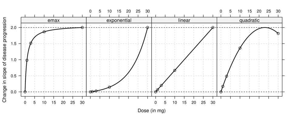
From discussions with the clinical team, the four candidate models displayed in Figure 4 were identified:

• Emax model with 90% of the maximum effect at 10 mg, corresponding to an ED${}_{50}=1.11$

• Quadratic model with maximum effect at 23 mg, corresponding to standardized model parameter $\delta=-0.022$

• Exponential model with 30% of the maximum effect occurring at 20 mg, corresponding to a standardized model parameter $\delta=8.867$

• Linear model

Figure 4: Candidate models for neurodenerative disease example.

For confidentiality reasons, the data from the actual trial cannot be used here, so we utilize a simulated dataset with characteristics similar to the original data with an Emax DR profile imposed on the linear slopes $\mu(x)$. Figure 5 shows the simulated data per dose, which is available in the DoseFinding package, in the neurodeg data set.

Figure 5: Simulated data for neurodegenerative disease example. Gray lines correspond to individual patient profiles, black line to loess smoother.

In what follows we illustrate the individual steps of MCPMod along with its implementation in DoseFinding package (version 0.9-6).

The $\widehat{{\boldsymbol{\mu}}}$ vector is estimated via an LME fit of data, which can be done, for example, using the lme function in the nlme R package, as illustrated below.

data(neurodeg)
head(neurodeg, n=3)
>       resp id dose time
> 1 191.7016  1    0    0
> 2 178.3995  1    0    3
> 3 167.3385  1    0    6
fm <- lme(resp ~ as.factor(dose):time, neurodeg, ~time|id)
muH <- fixef(fm)[-1] # extract estimates
covH <- vcov(fm)[-1,-1]

The estimated slopes are $\widehat{{\boldsymbol{\mu}}}=\left(-5.099,-4.581,-3.220,-2.879,-3.520\right)^{\prime}$ with corresponding estimated variance-covariance matrix with compound symmetry structure with diagonal elements $0.149$ and off-diagonal elements $0.0094$.

The optimal contrasts corresponding to the candidate models are calculated using the formula in (3), with ${{\boldsymbol{S}}}$ given by the estimated variance-covariance matrix of $\widehat{{\boldsymbol{\mu}}}$. The DoseFinding package includes the function optContr to calculate optimal contrasts based on (3) as follows.

doses <- c(0, 1, 3, 10, 30)
mod <- Mods(emax = 1.11, quadratic=-0.022, exponential = 8.867, linear = NULL,
            doses = doses) # definition of candidate shapes
contMat <- optContr(mod, S=covH) # calculate optimal contrasts

The MCTtest function in the DoseFinding package implements the optimal model contrast tests for $\widehat{{\boldsymbol{\mu}}}$ based on the multiple comparison approach described in Section 2.2.

MCTtest(doses, muH, S=covH, type = "general", critV = T, contMat=contMat)
> . . .
> Multiple Contrast Test:
>             t-Stat  adj-p
> emax         4.561 <0.001
> quadratic    3.680 <0.001
> linear       2.274 0.0249
> exponential  1.277 0.1818
>
> Critical value: 2.275 (alpha = 0.025, one-sided)

The Emax, quadratic and linear model contrasts are all significant, but the exponential model failed to reach significance. Therefore, the significance of a dose-response signal is established and we can move forward to estimating the dose-response profile and the target dose.

Two approaches can be used for model fitting in this example: the two-stage GLS non-linear dose-response fitting method described in Section 3, or mixed-effects modeling (linear and nonlinear) incorporating a parametric dose response model for the progression slope $\mu(x)$. We consider first the two-stage GLS method, which is implemented in the fitMod function in DoseFinding, illustrated in the call below for the Emax model.

fitMod(doses, muH, S=covH, model="emax", type = "general", bnds=c(0.1, 10))
> Dose Response Model
>
> Model: emax
> Fit-type: general
>
> Coefficients dose-response model
>     e0   eMax   ed50
> -5.181  2.180  1.187

The gAIC values (as discussed in Section 3.1) corresponding to the fits for the Emax, quadratic, and linear models are, respectively: 10.66, 11.07 and 24.22, indicating the better adequacy of the Emax model. Note that the DoseFinding package also includes an MCPMod function that performs MCTtest, model selection and model fitting in one step.

The mixed-effects model fit approach in this case is illustrated below for the Emax model using the nlme function

nlme(resp ~ b0 + (e0 + eM * dose/(ed50 + dose))*time, neurodeg,
     fixed = b0 + e0 + eM + ed50 ~ 1, random = b0 + e0 ~ 1 | id,
     start = c(200, -4.6, 1.6, 3.2))
...
  Fixed: b0 + e0 + eM + ed50 ~ 1
        b0         e0         eM       ed50
200.451303  -5.178739   2.181037   1.198791

The estimated fixed effects from the NLME model are quite close to the estimates obtained via the GLS two-stage method. The AIC values corresponding to the Emax, quadratic and linear models under the mixed-effects model fit are, respectively: 8352.60, 8353.10 and 8365.79 confirming the Emax as the best fitting model. It is intriguing to see how similar the differences in AIC between the different models are to the differences in gAIC values.

Estimates for the target dose, that is, the smallest dose producing an effect greater than or equal to the target value of 1.4, can be obtained with either of the model fitting approaches. The resulting estimated target doses are 2.13 under the two-stage GLS method and 2.15 under the NLME model. Alternatively, model averaging methods could have been used to estimate the target dose and the dose-response profile.

4.2 Binary and placebo-adjusted data

In this section we will go through two concrete examples on how to use the DoseFinding R package to apply MCPMod to binary data and placebo-adjusted normal data. Only the required R commands are given here, but not the output.

4.2.1 Binary endpoint

This example is based on trial NCT00712725 from clinicaltrials.gov. This was a randomized, placebo-controlled dose response trial for the treatment of acute migraine, with a total of 7 active doses ranging between 2.5mg and 200mg and placebo. The primary endpoint was “being pain free at 2 hours postdose”, i.e., a binary endpoint. The analysis presented here is a post-hoc analysis.

As a reasonable set of candidate models and contrasts, we select 4 different shapes of the sigmoid Emax model $f(x,{\boldsymbol{\theta}})=E_{0}+E_{max}x^{h}/(x^{h}+ED_{50}^{h})$, which cover a very wide range of monotonic shapes and a quadratic model to safeguard against the possibility of a unimodal dose response relationship. The Mods function is used for that, and one can also plot the candidate shapes.

doses <- c(0,2.5,5,10,20,50,100,200)
models <- Mods(sigEmax = rbind(c(2.5, 1),c(10,1),c(50, 3),c(100,2)),
               quadratic = -1/250, doses=doses)
plot(models)

The first stage of the two-step MCPMod approach consists of fitting a model with ANOVA-type parametrization to the data to obtain estimates $\widehat{{\boldsymbol{\mu}}}$ and its asymptotic covariance matrix ${\boldsymbol{S}}$. The logistic regression model is used here, which means that the candidate models are formulated on the logit scale (other scales could be used). The ANOVA logistic regression model can be fitted as follows.

## data from NCT00712725 study
dosesFact <- as.factor(doses) ## treat dose as categorical variable
N <- c(133, 32, 44, 63, 63, 65, 59, 58)
## % of patients painfree at 2h post-dose
RespRate <- c(13,4,5,16,12,14,14,21)/N
## fit logistic regression (without intercept)
logfit <- glm(RespRate~dosesFact-1, family = binomial, weights = N)
muHat <- coef(logfit)
S <- vcov(logfit)

Now all subsequent inference only depends on muHat and S obtained from the logistic regression. The multiple contrast test from 2.2 using optimal trend contrasts can be produced as follows

MCTtest(doses, muHat, S=S, models = models, type = "general")

All contrasts are significant. The modeling step can now be performed using the fitMod function. Here for illustration we fit the sigmoid Emax model and the quadratic model.

modSE <- fitMod(doses, muHat, S=S, model = "emax", type="general")
modQuad <- fitMod(doses, muHat, S=S, model = "quadratic", type = "general")
gAIC(modSE);gAIC(modQuad)

A comparison of the gAIC values reveals that the sigmoid Emax model provides a better fit than the quadratic model.

Above we performed the different steps of the MCPMod procedure separately. One could alternatively have used

MCPMod(doses, muHat, S=S, models=models, type = "general", Delta = 0.2)

directly.

4.2.2 Fitting on placebo-adjusted scale

For this example we use the IBScovars data set from the DoseFinding package, taken from [3]. The data are part of a dose ranging trial on a compound for the treatment of irritable bowel syndrome with four active doses 1, 2, 3, 4 equally distributed in the dose range $[0,4]$ and placebo. The primary endpoint was a baseline adjusted abdominal pain score with larger values corresponding to a better treatment effect. In total 369 patients completed the study, with nearly balanced allocation across the doses.

The endpoint is assumed to be normally distributed and it is of interest to adjust for the additive covariate gender. While the DoseFinding package can deal with this situation exactly, here we illustrate using the placebo-adjusted (effect) estimates. Note that, in the case of time-to-event data, one would proceed similarly. Here we only illustrate fitting an emax model, using the MCTtest and MCPMod functions is analogous to the calls in Section 4.2.1, but using the additional argument placAdj = TRUE. We plot the fitted model together with confidence intervals for the model fit and the ANOVA type effect estimates.

data(IBScovars)
anovaMod <- lm(resp~factor(dose)+gender, data=IBScovars)
drFit <- coef(anovaMod)[2:5] # placebo adjusted (=effect) estimates at doses
S <- vcov(anovaMod)[2:5,2:5] # estimated covariance
dose <- sort(unique(IBScovars$dose))[-1] # vector of active doses
## now fit an emax model to these estimates
gfit <- fitMod(dose, drFit, S=S, model = "emax", placAdj = TRUE,
               type = "general", bnds = c(0.01, 2))
plot(gfit, CI = TRUE, plotData = "meansCI")

5 Conclusions

The extended MCPMod methodology, together with its corresponding software implementation in the DoseFinding package in R, greatly broaden the scope of application of the original MCPMod approach. Most type of endpoints, and associated model-based analyses, utilized in dose finding studies can be handled in the context of the extended approach.

Further extensions of the approach discussed here are possible and of interest in practice. An increasing number of indications and drugs require regimen selection, in addition to the more traditional dose selection. Different approaches can be considered in the context of MCPMod, or its extension, discussed here. One could focus on estimating the exposure-response relationship, for example, combing dose and regimen into one model covariate. The much larger number of exposure values, compared to dose levels, could pose a problem for the derivation of optimal model contrasts and for the MCP step, more generally. Dose-time response modeling in the context of model uncertainty provide another venue for extending MCPMod. Further research is needed in those topics.

Model-based dose finding methods, such as the extended MCPMod, provide better understanding of the dose-response relationship, generally translating into more accurate dose selection for confirmatory trials. Realizing the full potential that these methods have to offer, however, requires changes in the way Phase II studies are traditionally designed. By and large, dose finding studies are planned as mini Phase III trials, using hypothesis tests to select the dose, or doses, to bring forward to the confirmatory stage. Relatively few doses (typically two active treatment arms and placebo) are used in such Phase II studies, making it hard to entertain any type of modeling. The sample size derivation in this type of studies is based on power calculations for detecting at least one dose significantly different from placebo. The resulting number of subjects is typically inadequate for proper estimation of target doses (and dose response modeling). A discussion of a different balance in resource allocation between Phases II and III, taking into account the overall probability of program success, is long overdue. Utilization of larger number of doses (e.g., 4 or 5), coupled with larger sample sizes, would go along way in enabling model-based methods to improve dose selection in Phase II and, as a result, the probability of success in Phase III.

Appendix A Derivation of Optimal Contrasts

In this section the closed form solution for the optimal contrasts for the case of a general covariance structure is derived. Optimality here refers to maximum power of the univariate contrast test, if a specified mean vector ${\boldsymbol{\mu}}$ (with corresponding positive definite covariance matrix ${\boldsymbol{S}}$) is true, which means that the non-centrality parameter

$$g(\mathbf{c},\boldsymbol{\mu})=\frac{\mathbf{c}^{\prime}{\boldsymbol{\mu}}}{\sqrt{{\boldsymbol{c}}^{\prime}{\boldsymbol{S}}{\boldsymbol{c}}}},$$

needs to be maximized with respect to ${\boldsymbol{c}}$, subject to ${\boldsymbol{c}}^{\prime}{\boldsymbol{1}}=0$.

Writing ${\boldsymbol{C}}_{0}=\left(-\mathbf{1}_{K-1}\vdots\mathbf{I}_{K-1}\right)$, the constrained maximization problem is equivalent to the unconstrained maximization of $\frac{\left(\mathbf{c}^{\prime}\mathbf{C_{0}\mu}\right)^{2}}{\mathbf{c}^{\prime}\mathbf{C_{0}SC_{0}}^{\prime}\mathbf{c}}$. This, however, is the solution to the generalized eigenvalue problem

$${\boldsymbol{C}}_{0}{\boldsymbol{\mu}}{\boldsymbol{\mu}}^{\prime}{\boldsymbol{C}}_{0}^{\prime}{\boldsymbol{x}}=\lambda\mathbf{C_{0}SC_{0}}^{\prime}{\boldsymbol{x}},$$

see e.g. [1], formula (2.66). As ${\boldsymbol{C}}_{0}{\boldsymbol{\mu}}{\boldsymbol{\mu}}^{\prime}{\boldsymbol{C}}_{0}^{\prime}$ is of rank 1, it has only a single non-zero eigenvalue. Thus, it is immediately clear that $\mathbf{c}=const\cdot(\mathbf{{\boldsymbol{C}}_{0}S{\boldsymbol{C}}_{0}^{\prime}})^{-1}{\boldsymbol{C}}_{0}{\boldsymbol{\mu}},const\neq 0$ is the only solution to the generalized eigenvalue problem. We further note that $\mathbf{c}=const\cdot(\mathbf{{\boldsymbol{C}}_{0}S{\boldsymbol{C}}_{0}^{\prime}})^{-1}{\boldsymbol{C}}_{0}{\boldsymbol{\mu}}=const\cdot{{\boldsymbol{S}}}^{-1}({\boldsymbol{\mu}}-\frac{{\boldsymbol{\mu}}^{\prime}{{\boldsymbol{S}}}^{-1}{\boldsymbol{1}}}{{\boldsymbol{1}}^{\prime}{{\boldsymbol{S}}}^{-1}{\boldsymbol{1}}}{\boldsymbol{1}})$. It is clear that the optimal solution is invariant with respect to addition or multiplication of any scalar constant to the vector ${\boldsymbol{\mu}}$, which is why one can also use the standardized mean vectors ${\boldsymbol{\mu}}^{0}_{m}$ instead of ${\boldsymbol{\mu}}$, which then gives the result in formula (3).

Appendix B Placebo-adjusted dose response modeling

In a few cases one would like to perform MCPMod on placebo-adjusted estimates, for example when there are (additive) covariates in the model, or when using a Cox PH model (where one can only obtain control-adjusted estimates). In what follows we will first demonstrate the equality of test statistics, and calculate optimal contrasts. Then

B.1 Test statistics and optimal contrasts

If we want to test a linear contrast of the responses per dose group, it does not matter whether we fit a placebo adjusted curve or include the placebo group as a response and then test contrasts to placebo.

To see this, consider the ANOVA estimate

$$\widehat{{\boldsymbol{\mu}}}\sim N({\boldsymbol{\mu}},{\boldsymbol{S}})$$ (9)

where the first component $\widehat{\mu}_{0}$ of the vector $\widehat{{\boldsymbol{\mu}}}$ corresponds to the placebo response. The test contrasts can then be produced by multiplication of $\widehat{{\boldsymbol{\mu}}}$ with the $(K-1)\times K$ contrast matrix ${\boldsymbol{C}}_{0}=\left(-\mathbf{1}_{K-1}\vdots\mathbf{I}_{K-1}\right)$, where ${\boldsymbol{1}}_{K-1}$ is a column vector of ones of size $K-1$ and ${\boldsymbol{I}}_{K-1}$ the $K-1$ dimensional identity matrix. We obtain the corresponding contrast

$$\widehat{{\boldsymbol{\mu}}}_{C}\sim N({\boldsymbol{\mu}}_{C},{\boldsymbol{S}}_{C})$$ (10)

with $\widehat{{\boldsymbol{\mu}}}_{C}={\boldsymbol{C}}_{0}\widehat{{\boldsymbol{\mu}}}$, ${\boldsymbol{\mu}}_{C}={\boldsymbol{C}}_{0}{\boldsymbol{\mu}}$ and ${\boldsymbol{S}}_{C}={\boldsymbol{C}}_{0}{\boldsymbol{S}}{\boldsymbol{C}}_{0}$.

The contrast test statistic in model (9) is of the form

$$m_{C}=\max\frac{\mathbf{c}^{\prime}\widehat{{\boldsymbol{\mu}}}}{\sqrt{\mathbf{c}^{\prime}\mathbf{S}\mathbf{c}}}\mbox{ subject to }\mathbf{c}^{\prime}\mathbf{1}_{K}=0,$$ (11)

with $\mathbf{c}$ such that $m_{C}$ attains a maximum. In model (10), the restriction on $\mathbf{c}$ is already absorbed in the matrix ${\boldsymbol{C}}_{0}$ and the test statistic takes the form

$$m_{P}=\max\frac{\mathbf{d}^{\prime}\mathbf{C}_{0}{\boldsymbol{\mu}}}{\sqrt{\mathbf{d}^{\prime}{\boldsymbol{C}}_{0}\mathbf{SC}_{0}^{\prime}\mathbf{d}}},$$ (12)

where $\mathbf{d}$ is no longer a contrast and again $\mathbf{d}$ is chosen such that $m_{P}$ is at its maximum. Now, it can be seen that $\mathbf{c}={\boldsymbol{C}}_{0}^{\prime}\mathbf{d}$: Setting $\mathbf{c}=\mathbf{C}_{0}^{\prime}\mathbf{d}$ implies $\mathbf{c}^{\prime}\mathbf{1}_{K}=0$, as ${\boldsymbol{C}}_{0}\mathbf{1}_{K}=0$. Hence, $m_{C}\geq m_{P}$. On the other hand, if $\mathbf{c}^{\prime}\mathbf{1}_{K}=0$, then there must be some $\mathbf{d}\in\mathbf{R}^{K-1}$ such that $\mathbf{c}$ can be written as $\mathbf{c}=\mathbf{C}_{0}^{\prime}\mathbf{d}$, since the rows of the $(K-1)\times K$-matrix $\mathbf{C}_{0}$ provide a base of the $(K-1)$-dimensional hyperspace orthogonal to $\mathbf{1}_{K}$ in $\mathbf{R}^{K}$. Consequently, $m_{C}\leq m_{P}$. It follows that $m_{C}=m_{P}$ and that if $\mathbf{d}$ maximizes (12), then $\mathbf{C}_{0}^{\prime}\mathbf{d}$ maximizes (11).

Specifically the optimal $\mathbf{d}^{opt}$ can be calculated as $\mathbf{d}^{opt}={\boldsymbol{S}}_{C}^{-1}{\boldsymbol{\mu}}_{C}$, as the sum to 0 constraint is removed.

B.2 Dose Response Model Fitting

In the two-stage generalized least squares fitting procedure one minimizes the criterion

$$(f({\boldsymbol{x}},{\boldsymbol{\theta}})-\widehat{{\boldsymbol{\mu}}})^{\prime}{\boldsymbol{S}}^{-1}(f({\boldsymbol{x}},{\boldsymbol{\theta}})-\widehat{{\boldsymbol{\mu}}}).$$ (13)

When we only have $\widehat{{\boldsymbol{\mu}}}_{C}$ one would not fit a full dose response model $\theta_{0}+\theta_{1}f^{0}(x,{\boldsymbol{\theta}}^{0})$ but work with a model without the intercept $\theta_{0}$. $f_{C}(x,{\boldsymbol{\theta}})=\theta_{1}f(x,{\boldsymbol{\theta}}^{0})$. The optimization criterion proposed for placebo-adjusted is then

$$(f_{C}(x,{\boldsymbol{\theta}})-\widehat{{\boldsymbol{\mu}}}_{C})^{\prime}{\boldsymbol{S}}_{C}^{-1}(f_{C}(x,{\boldsymbol{\theta}})-\widehat{{\boldsymbol{\mu}}}_{C}).$$ (14)

When $f^{0}(0,{\boldsymbol{\theta}}^{0})=0$ one can see that (13) and (14) are equal. This follows from the fact that (14) is equal to

$$({\boldsymbol{C}}_{0}(f({\boldsymbol{x}},{\boldsymbol{\theta}})-\widehat{{\boldsymbol{\mu}}}))^{\prime}({\boldsymbol{C}}_{0}{\boldsymbol{S}}{\boldsymbol{C}}_{0}^{\prime})^{-1}({\boldsymbol{C}}_{0}(f({\boldsymbol{x}},{\boldsymbol{\theta}})-\widehat{{\boldsymbol{\mu}}})),$$

and because ${\boldsymbol{C}}_{0}^{\prime}({\boldsymbol{C}}_{0}{\boldsymbol{S}}{\boldsymbol{C}}_{0}^{\prime})^{-1}{\boldsymbol{C}}_{0}={\boldsymbol{S}}^{-1}$ (which follows from multiplication from the left with ${\boldsymbol{C}}_{0}{\boldsymbol{S}}$).

Appendix C Proof of the result in section 3.1

Let ${\boldsymbol{\theta}}_{0}$ denote the true value of the parameter ${\boldsymbol{\theta}}$ and ${\boldsymbol{\mu}}_{0}={\boldsymbol{f}}({\boldsymbol{x}},{\boldsymbol{\theta}}_{0})$ where ${\boldsymbol{x}}$ is a known vector of fixed values. Assume that the following conditions are satisfied:

• There exists a symmetric, positive definite estimate ${\boldsymbol{S}}$ of the covariance matrix of $\widehat{{\boldsymbol{\mu}}}$ with $a_{n}{\boldsymbol{S}}\overset{P}{\rightarrow}{\boldsymbol{\Sigma}}$ for a positive nondecreasing sequence $a_{n}$ converging to $\infty$ as $n\rightarrow\infty$, and a positive definite, symmetric matrix ${\boldsymbol{\Sigma}}\in\mathbb{R}^{d\times d}$.

• If $N(0,{\boldsymbol{\Sigma}})$ denotes the multivariate normal distribution with mean 0 and covariance matrix ${\boldsymbol{\Sigma}}$, then ${a_{n}}^{1/2}(\widehat{{\boldsymbol{\mu}}}-{\boldsymbol{\mu}}_{0})\overset{d}{\rightarrow}N(0,{\boldsymbol{\Sigma}})$, where $\overset{d}{\rightarrow}$ denotes convergence in distribution. As a consequence of $a_{n}\rightarrow\infty$, the estimate $\widehat{{\boldsymbol{\mu}}}$ is consistent, i.e., $\widehat{{\boldsymbol{\mu}}}\overset{P}{\rightarrow}{\boldsymbol{\mu}}_{0}$ (see e.g. Serfling, 1980, p.26).

• The mapping ${\boldsymbol{\Theta}}\mapsto\mathbb{R}^{k}$, ${\boldsymbol{\theta}}\mapsto{\boldsymbol{f}}({\boldsymbol{x}},{\boldsymbol{\theta}})$, with ${\boldsymbol{x}}\in\mathbb{R}^{k}$ is a bijective function of ${\boldsymbol{\theta}}$ which is twice differentiable in an open region around ${\boldsymbol{\theta}}_{0}$.

Under these assumptions $\widehat{{\boldsymbol{\theta}}}$ is a consistent estimator of ${\boldsymbol{\theta}}$, i.e., $\widehat{{\boldsymbol{\theta}}}\overset{P}{\rightarrow}{\boldsymbol{\theta}}$ and $\sqrt{a_{n}}(\widehat{{\boldsymbol{\theta}}}-{\boldsymbol{\theta}}_{0})\overset{d}{\rightarrow}N({\boldsymbol{0}},{\boldsymbol{B}}({\boldsymbol{\theta}}_{0})^{\prime}{\boldsymbol{M}}({\boldsymbol{\theta}}_{0}){\boldsymbol{B}}({\boldsymbol{\theta}}_{0}))$, where ${\boldsymbol{M}}({\boldsymbol{\theta}})={\boldsymbol{F}}({\boldsymbol{\theta}})^{\prime}{\boldsymbol{A}}{\boldsymbol{\Sigma}}{\boldsymbol{A}}{\boldsymbol{F}}({\boldsymbol{\theta}})$ and ${\boldsymbol{B}}({\boldsymbol{\theta}})=({\boldsymbol{F}}({\boldsymbol{\theta}})^{\prime}{\boldsymbol{A}}{\boldsymbol{F}}({\boldsymbol{\theta}}))^{-1}$.

Proof:

Let $\widehat{{\boldsymbol{\Psi}}}({{\boldsymbol{\theta}}})=(\widehat{{\boldsymbol{\mu}}}-{\boldsymbol{f}}({\boldsymbol{x}},{\boldsymbol{\theta}}))^{\prime}{{\boldsymbol{A}}_{n}}(\widehat{{\boldsymbol{\mu}}}-{\boldsymbol{f}}({\boldsymbol{x}},{\boldsymbol{\theta}}))$ and ${{\boldsymbol{\Psi}}}({{\boldsymbol{\theta}}})=({{\boldsymbol{\mu}}}-{\boldsymbol{f}}({\boldsymbol{x}},{\boldsymbol{\theta}}))^{\prime}{{\boldsymbol{A}}}({{\boldsymbol{\mu}}}-{\boldsymbol{f}}({\boldsymbol{x}},{\boldsymbol{\theta}}))$.

First we note that consistency of the estimator is easy to establish using standard theory for the consistency of M-estimators. For example the three conditions in Theorem 5.7 from [39] are easy to verify (A1)-(A3).

The proof of the distribution of $\sqrt{a_{n}}(\widehat{{\boldsymbol{\theta}}}-{\boldsymbol{\theta}}_{0})\overset{d}{\rightarrow}N({\boldsymbol{0}},{\boldsymbol{B}}({\boldsymbol{\theta}}_{0})^{\prime}{\boldsymbol{M}}({\boldsymbol{\theta}}_{0}){\boldsymbol{B}}({\boldsymbol{\theta}}_{0}))$ works along the lines of [33, ch. 12.2.3], which we restate here with the modifications needed for our situation.
As $\widehat{{\boldsymbol{\theta}}}$ minimizes $\widehat{{\boldsymbol{\Psi}}}({\boldsymbol{\theta}})$, we have$\frac{d\widehat{{\boldsymbol{\Psi}}}(\widehat{{\boldsymbol{\theta}}})}{d{\boldsymbol{\theta}}}=0$. Thus, by the mean value theorem, there is a $\widetilde{{\boldsymbol{\theta}}}$ between ${\boldsymbol{\theta}}_{0}$ and $\widehat{{\boldsymbol{\theta}}}$ such that

$$0=\frac{d\widehat{{\boldsymbol{\Psi}}}({\boldsymbol{\theta}}_{0})}{d{\boldsymbol{\theta}}}+\frac{d^{2}\widehat{{\boldsymbol{\Psi}}}(\widetilde{{\boldsymbol{\theta}})}}{d{\boldsymbol{\theta}}d{\boldsymbol{\theta}}^{\prime}}({\boldsymbol{\theta}}_{0}-\widehat{{\boldsymbol{\theta}}}).$$

Hence

$$\sqrt{a_{n}}(\widehat{{\boldsymbol{\theta}}}-{\boldsymbol{\theta}}_{0})=\sqrt{a_{n}}(\frac{d^{2}\widehat{{\boldsymbol{\Psi}}}(\widetilde{{\boldsymbol{\theta}})}}{d{\boldsymbol{\theta}}d{\boldsymbol{\theta}}^{\prime}})^{-1}(\frac{d\widehat{{\boldsymbol{\Psi}}}({\boldsymbol{\theta}}_{0})}{d{\boldsymbol{\theta}}}).$$ (15)

We now show that (i) $\sqrt{a_{n}}\frac{d\widehat{{\boldsymbol{\Psi}}}({\boldsymbol{\theta}}_{0})}{d{\boldsymbol{\theta}}}$ is asymptotically normal, and that (ii) $\left(\frac{d^{2}\widehat{{\boldsymbol{\Psi}}}(\widetilde{{\boldsymbol{\theta}})}}{d{\boldsymbol{\theta}}d{\boldsymbol{\theta}}^{\prime}}\right)^{-1}$ converges in probability to a non-singular matrix.

(i)

$$\frac{d\widehat{{\boldsymbol{\Psi}}}({{\boldsymbol{\theta}}})}{d{\boldsymbol{\theta}}}=-2{\boldsymbol{F}}({\boldsymbol{\theta}}){\boldsymbol{A}}_{n}(\widehat{{\boldsymbol{\mu}}}-{\boldsymbol{f}}({\boldsymbol{x}},{\boldsymbol{\theta}})),$$

where ${\boldsymbol{F}}({\boldsymbol{\theta}})$ is the $d\times k$ matrix of partial derivatives $\frac{df(x_{i},{\boldsymbol{\theta}})}{d\theta_{h}}$. ($i=1,...,k$,$\quad h=1,...,d$).

Since $\sqrt{a_{n}}\left(\widehat{{\boldsymbol{\mu}}}-{\boldsymbol{f}}({\boldsymbol{x}},{\boldsymbol{\theta}}_{0})\right)\overset{d}{\rightarrow}N({\boldsymbol{0}},{\boldsymbol{\Sigma}})$,

$$\sqrt{a_{n}}\frac{d\widehat{{\boldsymbol{\Psi}}}({\boldsymbol{\theta}}_{0})}{d{\boldsymbol{\theta}}}=-2\sqrt{a_{n}}{\boldsymbol{F}}({\boldsymbol{\theta}}_{0}){\boldsymbol{A}}_{n}\left(\widehat{{\boldsymbol{\mu}}}-{\boldsymbol{f}}({\boldsymbol{x}},{\boldsymbol{\theta}}_{0})\right)\overset{d}{\rightarrow}N({\boldsymbol{0}},4{\boldsymbol{F}}({\boldsymbol{\theta}}_{0}){\boldsymbol{A}}{\boldsymbol{\Sigma}}{\boldsymbol{A}}^{\prime}{\boldsymbol{F}}({\boldsymbol{\theta}}_{0})^{\prime})$$

.

(ii) Differentiate the second term twice to get

$$\frac{d^{2}\widehat{{\boldsymbol{\Psi}}}(\widetilde{{\boldsymbol{\theta}})}}{d{\boldsymbol{\theta}}d{\boldsymbol{\theta}}^{\prime}}=-2({\boldsymbol{U}}-{\boldsymbol{F}}(\widetilde{{\boldsymbol{\theta}}}){\boldsymbol{A}}_{n}{\boldsymbol{F}}(\widetilde{{\boldsymbol{\theta}}})^{\prime}),$$

where ${\boldsymbol{U}}$ is the $d\times d$ matrix with $h$-th column given by

$$\frac{d^{2}f({\boldsymbol{x}},{\boldsymbol{\theta}})}{d\theta_{h}d{\boldsymbol{\theta}}^{\prime}}{\boldsymbol{A}}_{n}(\widehat{{\boldsymbol{\mu}}}-{\boldsymbol{f}}({\boldsymbol{x}},\widetilde{{\boldsymbol{\theta}})}).$$

Now $\widehat{{\boldsymbol{\mu}}}\overset{P}{\rightarrow}{\boldsymbol{f}}({\boldsymbol{x}},{\boldsymbol{\theta}}_{0})$ and $\widehat{{\boldsymbol{\theta}}}\overset{P}{\rightarrow}\widetilde{{\boldsymbol{\theta}}}\overset{P}{\rightarrow}{\boldsymbol{\theta}}_{0}$, so all entries of ${\boldsymbol{U}}$ converge to 0. In total we get

$$\frac{d^{2}\widehat{{\boldsymbol{\Psi}}}(\widetilde{{\boldsymbol{\theta}})}}{d{\boldsymbol{\theta}}d{\boldsymbol{\theta}}^{\prime}}\overset{P}{\rightarrow}2{\boldsymbol{F}}({\boldsymbol{\theta}}_{0}){\boldsymbol{A}}{\boldsymbol{F}}({\boldsymbol{\theta}}_{0})^{\prime}$$

Defining ${\boldsymbol{M}}({\boldsymbol{\theta}})={\boldsymbol{F}}({\boldsymbol{\theta}}){\boldsymbol{A}}{\boldsymbol{\Sigma}}{\boldsymbol{A}}^{\prime}{\boldsymbol{F}}({\boldsymbol{\theta}})^{\prime}$ and ${\boldsymbol{B}}({\boldsymbol{\theta}})=({\boldsymbol{F}}({\boldsymbol{\theta}}){\boldsymbol{A}}{\boldsymbol{F}}({\boldsymbol{\theta}})^{\prime})^{-1}$ and inserting the results from (i) and (ii) into (15), one obtains that the asymptotic distribution of $\sqrt{a_{n}}(\widehat{{\boldsymbol{\theta}}}-{\boldsymbol{\theta}}_{0})$ is $N({\boldsymbol{0}},{\boldsymbol{B}}({\boldsymbol{\theta}}_{0})^{\prime}{\boldsymbol{M}}({\boldsymbol{\theta}}_{0}){\boldsymbol{B}}({\boldsymbol{\theta}}_{0}))$. $\Box$

Appendix D Additional Plots

Figure 6: Time-To-Event endpoint

Figure 7: Binary endpoint

Figure 8: Normal endpoint

Figure 9: Root mean squared error for estimating the dose response (averaged over the doses available), count endpoint.

Figure 10: Root mean squared error for estimating the dose response (averaged over the doses available), time-to-event endpoint.

Figure 11: Root mean squared error for estimating the dose response (averaged over the doses available), binary endpoint.

References

- [1] H. Ahrens and J. Läuter. Mehrdimensionale Varianzanalyse. Akademie-Verlag, Berlin, 1981.
- [2] D. M. Bates and D. G. Watts. Nonlinear Regression Analysis and Applications. John Wiley and sons, New York, 1988.
- [3] E. Biesheuvel and L. A. Hothorn. Many-to-one comparisons in stratified designs. Biometrical Journal, 44:101–116, 2002.
- [4] B Bornkamp, F Bretz, H Dette, and J C Pinheiro. Response-adaptive dose-finding under model uncertainty. Annals of Applied Statistics, 5:1611–1631, 2011.
- [5] B Bornkamp, Frank Bretz, Alex Dmitrienko, Greg Enas, Brenda Gaydos, Chyi-Hung Hsu, Franz König, Michael Krams, Qing Liu, Beat Neuenschwander, Tom Parke, José C Pinheiro, Amit Roy, Rick Sax, and Frank Shen. Innovative approaches for designing and analyzing adaptive dose-ranging trials. Journal of Biopharmaceutical Statistics, 17:965–995, 2007.
- [6] Bjoern Bornkamp, Jose Pinheiro, and Frank Bretz. DoseFinding: Planning and Analyzing Dose Finding experiments, 2013.
- [7] Bj“orn Bornkamp, Jos’e C. Pinheiro, and Frank Bretz. MCPMod: An R package for the design and analysis of dose-finding studies. Journal of Statistical Software, 29(7):1–23, 2009.
- [8] F. Bretz and L. Hothorn. Statistical analysis of monotone or non-monotone dose-response data from in-vitro toxicological assays. Alternatives to Laboratory Animals, 31 Supplement 1:81–96, 2003.
- [9] F. Bretz, W. Maurer, W. Brannath, and M. Posch. A graphical approach to sequentially rejective multiple test procedures. Statistics in Medicine, 28:586–604, 2009.
- [10] Frank Bretz, José C. Pinheiro, and Michael Branson. Combining multiple comparisons and modeling techniques in dose-response studies. Biometrics, 61:738–748, 2005.
- [11] S. T. Buckland, K. P. Burnham, and N. H. Augustin. Model selection an integral part of inference. Biometrics, 53:603–618, 1997.
- [12] S. Chevret. Statistical methods for dose finding experiments. Wiley, 2006.
- [13] P Diggle, Patrick Heagerty, Kung-Yee Liang, and Scott Zeger. Analysis of Longitudinal Data. Oxford University Press, 1994.
- [14] A. J. Dobson. An introduction to generalized linear models. Chapman and Hall, Boca Raton, 2002.
- [15] V. Dragalin, F. Hsuan, and S. K. Padmanabhan. Adaptive designs for dose-finding studies based on the sigmoid emax model. Journal of Biopharmaceutical Statistics, 17:1051–1070, 2007.
- [16] Vladimir Dragalin, Björn Bornkamp, Frank Bretz, Frank Miller, S. Krishna Padmanabhan, Nitin Patel, Inna Perevozskaya, Jose Pinheiro, and Jonathan R. Smith. A simulation study to compare new adaptive dose-ranging designs. Statistics in Biopharmaceutical Research, 2:487–512, 2010.
- [17] A. Genz and F. Bretz. Computation of Multivariate Normal and t Probabilities. Springer, 2009.
- [18] D. Hoel and C. Portier. Nonlinearity of dose-response functions for carcinogenicity. Enrironmental Health Perspectives, 102 Supplement 1:109–113, 1994.
- [19] T Hothorn, F Bretz, and P Westfall. Simultaneous inference in general parametric models. Biometrical Journal, 50:346–363, 2008.
- [20] Chyi-Hung Hsu. Evaluating potential benefits of dose-exposure-response modeling for dose finding. Pharmaceutical Statistics, 8:203–215, 2009.
- [21] P. J. Huber. The behavior of maximum likelihood estimates under nonstandard conditions. Proceedings of the Fifth Berkeley Symposium on Mathematical Statistics and Probability, Vol. I, pages 221–233, 1967.
- [22] ICH. ICH Topic E4: Dose-response information to support drug registration, E4 1994.
- [23] B Jones, G Layton, H Richardson, and N Thomas. Model-based Bayesian adaptive dose-finding designs for a phase II trial. Statistics in Biopharmaceutical Research, 3:276–287, 2011.
- [24] R. Krishna. Dose optimization in drug development. Informa Healthcare, 2006.
- [25] Dan Lin, Ziv Shkedy, Daniel Yekutieli, Dhammika Amaratunga, and Luc Bijnens. Modeling Dose-response Microarray Data in Early Drug Development Experiments With R. Spinger, 2012.
- [26] B. Neuenschwander, M. Branson, and T. Gsponer. Critical aspects of the Bayesian approach to phase I cancer trials. Statistics in Medicine, 27:2420–2439, 2008.
- [27] S. D. Peddada and J. K. Haseman. Analysis of nonlinear regression models: A cautionary note. Dose-Response, pages 342–352, 2005.
- [28] J Pinheiro, F Sax, Z Antonijevic B Bornkamp, F Bretz, C Chuang-Stein, V Dragalin, P Fardipour, P Gallo, W Gillespie, C Hsu, F Miller S Padmanabhan, N Patel, I Perevozskaya, A Roy, A Sanil, and J Smith. Adaptive and model-based dose-ranging trials: Quantitative evaluation and recommendations. white paper of the phrma working group on adaptive dose-ranging studies (with discussion). Statistics in Biopharmaceutical Research, 2:435–454, 2010.
- [29] J. C. Pinheiro, B. Bornkamp, and F. Bretz. Design and analysis of dose finding studies combining multiple comparisons and modeling procedures. Journal of Biopharmaceutical Statistics, 16:639–656, 2006.
- [30] J. C. Pinheiro, F. Bretz, and M. Branson. Analysis of dose-response studies – modeling approaches. In Naitee Ting, editor, Dose Finding in Drug Development, pages 146–171. Springer, New York, 2006.
- [31] Stephen J. Ruberg. Dose response studies. I. Some design considerations. Journal of Biopharmaceutical Statistics, 5(1):1–14, 1995.
- [32] Stephen J. Ruberg. Dose response studies. II. Analysis and interpretation. JBS, 5(1):15–42, 1995.
- [33] G. A. F. Seber and C. J. Wild. Nonlinear Regression. John Wiley and Sons, 1989.
- [34] W. H. Stewart and S. Ruberg. Detecting dose-response with contrasts. Statistics in Medicine, 19:913–921, 2000.
- [35] A. C. Tamhane, Yosef Hochberg, and C. W. Dunnett. Multiple test procedures for dose finding. Biometrics, 52:21–37, 1997.
- [36] Neal Thomas. Hypothesis testing and Bayesian estimation using a sigmoid Emax model applied to sparse dose designs. Journal of Biopharmaceutical Statistics, 16:657–677, 2006.
- [37] Naitee Ting. Dose finding in drug development. Spinger, 2006.
- [38] J. W. Tukey, J. L. Ciminera, and J. F. Heyse. Testing the statistical certainty of a response to increasing doses of a drug. Biometrics, 41:295–301, 1985.
- [39] A. W. van der Vaart. Asymptotic Statistics. Cambridge University Press, 1998.