Warm Spitzer Photometry of Three Hot Jupiters: HAT-P-3b, HAT-P-4b and HAT-P-12b

Abstract

We present Warm Spitzer/IRAC secondary eclipse time series photometry of three short-period transiting exoplanets, HAT-P-3b, HAT-P-4b and HAT-P-12b, in both the available 3.6 and 4.5 $\mu$m bands. HAT-P-3b and HAT-P-4b are Jupiter-mass, objects orbiting an early K and an early G dwarf stars, respectively. For HAT-P-3b we find eclipse depths of $0.112\%^{+0.015\%}_{-0.030\%}$ (3.6 $\mu$m) and $0.094\%^{+0.016\%}_{-0.009\%}$ (4.5 $\mu$m). The HAT-P-4b values are $0.142\%^{+0.014\%}_{-0.016\%}$ (3.6 $\mu$m) and $0.122\%^{+0.012\%}_{-0.014\%}$(4.5 $\mu$m). The two planets’ photometry is consistent with inefficient heat redistribution from their day to night sides (and low albedos), but it is inconclusive about possible temperature inversions in their atmospheres. HAT-P-12b is a Saturn-mass planet and is one of the coolest planets ever observed during secondary eclipse, along with hot Neptune GJ 436b and hot Saturn WASP-29b. We are able to place 3$\sigma$ upper limits on the secondary eclipse depth of HAT-P-12b in both wavelengths: $<0.042\%$ (3.6 $\mu$m) and $<0.085\%$ (4.5 $\mu$m). We discuss these results in the context of the Spitzer secondary eclipse measurements of GJ 436b and WASP-29b. It is possible that we do not detect the eclipses of HAT-P-12b due to high eccentricity, but find that weak planetary emission in these wavelengths is a more likely explanation. We place 3$\sigma$ upper limits on the $|e\,\cos\omega|$ quantity (where $e$ is eccentricity and $\omega$ is the argument of periapsis) for HAT-P-3b ($<0.0081$) and HAT-P-4b ($<0.0042$), based on the secondary eclipse timings.

1. Introduction

There are about 177 confirmed exoplanets with orbital periods of less than 10 days and masses greater than 0.1 Jupiter mass, which are often referred to as “hot Jupiters”. About 145 of them transit their host stars. Hot Jupiters have high equilibrium temperatures, often over 1000 K, due to their proximity to their parent stars. These planets make ideal targets for the Spitzer Space Telescope, which can directly detect their thermal emission via time series photometry in the infra-red during secondary eclipse.

The drop of total light from the planet-star system as the planet moves behind the star was first measured independently by Charbonneau et al. (2005) and Deming et al. (2005). By measuring the eclipse depth in several photometric bands, one can construct a very low resolution emergent spectrum of the observed planet in the infrared (Charbonneau et al., 2008; Grillmair et al., 2008). Comparison of similar spectra with models has suggested that there are two types of hot Jupiter atmospheres based on the presence or absence of temperature inversions in their upper layers (e.g., Knutson et al., 2008; Machalek et al., 2009; Todorov et al., 2010; Beerer et al., 2011; Deming et al., 2011; Todorov et al., 2012).

The mechanisms that create such inversions are not well established, but it is generally believed that planets with an inverted atmosphere have an additional opacity source in their atmospheres’ upper layers, where the pressure falls below $\sim 0.01$ bar (Burrows et al., 2008; Fortney et al., 2008). In the past, this opacity source has been suggested to be gas phase TiO (Hubeny et al., 2003; Burrows et al., 2007, 2008; Fortney et al., 2006a, 2008). However, this molecule may form grains on the night sides and in cold traps deep in the atmospheres on the day sides of some hot Jupiters with inversions such as HD 209458b, where the pressure-temperature profiles are expected to cross the condensation curve of TiO (Spiegel et al., 2009). In addition, TrES-3 is sufficiently heated to have gas phase TiO in its atmosphere, yet has no temperature inversion (Fressin et al., 2010), while XO-1b is too cool to maintain it, but appears to have an inverted atmosphere (Machalek et al., 2008). On the other hand, a more recent 3D mixing study of hot Jupiter atmospheres (Parmentier et al., 2013) has shown that TiO may stay aloft in HD 209458b’s atmosphere due to strong vertical mixing, if it forms grains no larger than several microns. According to this investigation, TiO in the form of larger particles should be depleted by the day-night cold trap. Thus, the role of TiO in the formation of temperature inversions remains controversial.

There are at least two alternative explanations for the presence or absence of temperature inversions. Zahnle et al. (2009) suggested that sulfur compounds may account for the stratospheric opacity in some hot Jupiter atmospheres. Another hypothesis is that the presence or absence of temperature inversions is correlated with the magnetic activity and related UV flux from the host star (Knutson et al., 2010). According to this idea, the increased UV flux received by planets orbiting active stars destroys the molecule responsible for the formation of temperature inversions.

We can test these hypotheses by building up a large sample of hot Jupiters with secondary eclipse measurements and search for correlations with other system parameters, such as stellar activity or the Ti abundance in the stellar photosphere. Although the Spitzer Space Telescope exhausted the last of its cryogen in May 2009, it still remains the best facility for carrying out these observations. The observatory has continued operating at a higher temperature of approximately 29 K, cooled by passive radiation. Only two photometric bands are still available, the 3.6 and 4.5 $\mu$m channels of the Infra-Red Array Camera (IRAC, Fazio et al., 2004). Fortunately, measurements in these two bands are often sufficient to constrain the presence or absence of temperature inversion in the upper layers of hot Jupiters (Knutson et al., 2010).

The energy budget is another aspect of transiting hot Jupiters that can be studied via secondary eclipse photometry. These planets are expected to tidally evolve within $\sim 1$ Gyr of their formation, and their rotation periods should become equal to their orbital periods, assuming zero eccentricity (Correia & Laskar, 2010). The transfer of heat from the day side to the night side can have strong influence on the emergent wavelength dependent flux of the day side of the planet, which is measured directly by estimating the secondary eclipse depth at a given wavelength. Relating observations to atmospheric models can place constraints on the heat redistribution efficiency and the Bond albedo of the planet (Cowan & Agol, 2011). The authors of this study suggest that planets with very high equilibrium temperatures have a narrow range of $\rm T_{d}/T_{0}$, where $\rm T_{d}$ is the effective dayside temperature and $\rm T_{0}$ is the equilibrium temperature at the substellar point. This ratio is a measure of the redistribution efficiency of the atmosphere, which Cowan & Agol (2011) find to be uniformly low for the hottest planets, while cooler planets appear to exhibit higher range of heat redistribution efficiencies and/or albedos.

In this paper we present Warm Spitzer time series photometry of three short period transiting exoplanets – HAT-P-3b (Torres et al., 2007), HAT-P-4b (Kovács et al., 2007) and HAT-P-12b (Hartman et al., 2009). The physical properties of the systems are listed in Table 1. In a previous paper (Todorov et al., 2012), we focused on Warm Spitzer secondary eclipse photometry of three planets (XO-4b, HAT-P-6b and HAT-P-8b) with masses comparable to Jupiter’s, orbiting F dwarfs. The magnetic activity of stars as indicated by the Ca II H&K line strengths is uncalibrated for effective temperatures over 6200 K or under 4200 K (Noyes et al., 1984). Since the host stars of all three of these targets were above or close to the 6200 K boundary, our results did not reliably test the correlation between magnetic activity of the host star and the atmospheric inversions proposed by Knutson et al. (2010), which relies on Ca II H&K line measurements for assessing the magnetic activity of the stars.

Therefore, in order to better cover the available parameter space, for this analysis we have chosen planets that orbit host stars with effective temperatures within the 4200—6200 K range. Our targets are less massive than Jupiter (the least massive, HAT-P-12b, has a mass similar to Saturn’s), but have radii similar to Jupiter’s. In addition to the secondary eclipse depth measurements, we combine their timings with the most precise ephemerides available (HAT-P-3, HAT-P-4: Sada et al. (2012), HAT-P-12: this paper) to constrain the orbital eccentricity of the planets.

For this analysis, we update the code developed by Todorov et al. (2012), to make use of full array mode observations (in the cases of HAT-P-4 and HAT-P-12) and variable aperture photometry (Lewis et al., 2013). We estimated the uncertainty of the eclipse depth and timing with the Markov Chain Monte Carlo and prayer-bead algorithms. It is in principle possible to use this code to analyze all available Spitzer secondary eclipse data sets in a single investigation, but we find that every data set has peculiarities that need to be addressed on individual basis. We analyze and report eclipse results for hot Jupiters in groups of three because this allows for the efficiency of analyzing data for multiple exoplanets, while retaining the ability to cope with the quirks of individual data sets.

In Section 2 we present the Spitzer observations and our photometry procedures. The details of the time series analysis and the uncertainty estimation are presented in Section 3. We discuss our results in the context of previous studies in Section 4.

2. Observations and Photometry

2.1. Secondary Eclipse Observations with Spitzer

We observed the secondary eclipses using the Infra-Red Array Camera (IRAC) on the Spitzer Space Telescope in both the 3.6 $\rm{\mu}$m and the 4.5 $\rm{\mu}$m channels. The observations on the HAT-P-3 system in both pass-bands utilized the IRAC subarray mode, resulting in $32\times 32$ pixel (39″$\times 39$″) images, centered on the planet’s host star. The HAT-P-4 and HAT-P-12 data are in full array mode, where each image is taken has the full IRAC resolution of $256\times 256$ pixels (5.2′$\times$5.2′).

The subarray mode images are stacked in FITS data cubes that contain 64 exposures taken in a sequence. Our HAT-P-3 observations have effective exposure times per image of 1.92 s in both pass-bands. The full array data have effective exposure times of 4.4 s (HAT-P-4) and 10.4 s (HAT-P-12) per image respectively in both wavelengths. Each secondary eclipse observation of HAT-P-3b lasted for 7 h 42 min resulting in 13,760 images (215 data cubes). The observations of HAT-P-4b covered 7 h 38 min, resulting in 3,871 images in each wavelength, while those of HAT-P-12b lasted almost as long – 7 h 37 min – but resulted in only 2,097 images per pass-band, due to the longer exposure time.

Complete information about the time span of the observations is presented in Table 3.

2.2. Photometry and Time Information Extraction

Our time-stamp extraction routine is very similar to the one used by Todorov et al. (2012). In all data sets, we perform the extraction on the Basic Calibrated Data (BCD) files produced by version S18.18.0 of the Spitzer pipeline. For timing of the photometric points, we rely on the $\rm{MJD\_OBS}$ keyword in the FITS headers, corrected to indicate the mid-exposure time. We convert this time stamp, given in modified Julian date, based on the Coordinated Universal Time (UTC) standard ($\rm MJD_{UTC}$), to Barycentric Julian Date based on the Terrestrial Time standard (BJD_TT) using Jason Eastman’s IDL routine get_spitzer_bjd (Eastman et al., 2010). We prefer to use the TT standard rather than UTC, because the latter is discontinuous and has leap seconds introduced occasionally. At the time of our observations, $\rm TT\approx UTC+$66.184$\,s$.

We convert the pixel intensities from $\rm MJy/sr$ to electron counts using the the information provided in the image headers, in order to be able to estimate the Poisson noise of the photometry. The data are filtered for energetic particle hits by following each pixel through time. This is done in two passes, first flagging all pixels 8 $\sigma$ or more away from a boxcar median through time with width 5. Their values are replaced with the local boxcar median value. In the second pass, all values more than 4 $\sigma$ away from the boxcar median through time (again with width 5) are flagged and their values are replaced with the local median value. For the HAT-P-3 data, this procedure is performed separately for each data cube instead of for the whole time series in order to avoid pixel rejection due to the sharp changes in background that occur between the last frame from one cube and the first frame from the next. This effect is similar to the one seen by Deming et al. (2011). The fraction of corrected pixels is about 0.53% (HAT-P-3, at 3.6 $\rm{\mu}$m), 0.12% (HAT-P-3, at 4.5 $\rm{\mu}$m), 0.13% (HAT-P-4, at both channels), 0.22% (HAT-P-12, at 3.6 $\rm{\mu}$m) and 0.24% (HAT-P-12, at 4.5 $\rm{\mu}$m).

We estimate the background flux from the full-array images by creating a histogram of all pixel values for each frame and fitting a Gaussian function. We correct for contamination by field stars and energetic particle hits by fitting only to the central portion of the histogram and excluding the regions that account for the high photon count pixels. We test for variable background across the full-array images by measuring the background based on 30$\times$30, 50$\times$50, and 100$\times$100 pixel boxes centered on the star-planet system (which was always positioned in the center of the array). Removing the background from the photometry in this manner produces at most 0.7% change in the photometric scatter around a running median of width 20 of the photometry compared to data reduction using the whole array to estimate background, in all data sets. This is marginal, therefore, we elect to maximize our background determination precision and use the whole array to determine the background levels. Since the subarray mode observations of HAT-P-3 result in only $32\times 32$ pixel images, we exclude a $5\times 5$ pixel square centered on the star from the histograms for these data, in order to avoid biasing the background estimation to higher values.

In order to locate the centroid of the stellar point response function (PRF) we experiment with fitting a two-dimensional Gaussian function to the core of the stellar image (Agol et al., 2010) and with flux-weighted centroiding (e.g., Charbonneau et al., 2008; Knutson et al., 2008). We find that in most cases there is an improvement in the standard deviation of the residuals that remain after we subtract our best fit model from the photometry, if we adopt flux-weighted centroiding. The only exception is the HAT-P-3b 4.5$\mu$m data set, where the difference in the resulting scatter is marginal ($\sim 0.1\%$). Therefore, we adopt flux-weighted centroiding for all data sets in this analysis.

We experiment with two different photometry approaches. First, we perform aperture photometry, using the IDL routine aper, varying the aperture radius in increments of 0.5 pixels between 1.5 and 6.5 pixels. We select the best photometry aperture radius by measuring the true scatter it produces around a boxcar median of the raw light curve with width 20. The scatter is not strongly correlated with aperture radius. For the HAT-P-3 subarray mode data, the minimum scatter is found at 2.5px (3.6 $\mu$m) and 3.0px (4.5 $\mu$m) pixel radii. For the full array mode data we find that the smallest scatter occurs at pixel radii of 4.0px (HAT-P-4, 3.6 $\mu$m), 3.0px (HAT-P-4, 4.5 $\mu$m), 5.0px (HAT-P-12, 3.6 $\mu$m) and 2.5px (HAT-P-12, 4.5 $\mu$m).

Separately, we perform photometry on all data by using time-variable aperture. For each image, we estimate the noise-pixel parameter (Mighell, 2005; Knutson et al., 2012; Lewis et al., 2013), which is a measure of the width of the stellar point spread function (PSF). It is defined in Section 2.2.2 of the Spitzer/IRAC instrument handbook as:

$$\tilde{\beta}=\frac{(\Sigma_{i}{I_{i}})^{2}}{\Sigma_{i}{I_{i}^{2}}},$$ (1)

where $I_{i}$ is the intensity detected by the $i^{th}$ pixel. The noise pixel parameter, $\tilde{\beta}$, is proportional to the full-width-half-maximum of the stellar PSF (Mighell, 2005). For each image, we calculate the photometric aperture radius:

$$r=\sqrt{\tilde{\beta}}b+c,$$ (2)

where b is a scaling factor and c is a constant. In each image frame, we measure the flux used to determine $\tilde{\beta}$ using circular aperture radii between 1.0 and 6.5 pixels. If any part of a pixel falls within the aperture radius, it is fully included in the $\tilde{\beta}$ calculation. For each of these values, we vary $b$ and $c$ in steps of 0.05. We fit each of the resulting light curves with our “systematics-and-eclipse” model and find the combination of photometric parameters that yields the smallest standard deviation of the residuals.

For the 3.6$\mu$m data sets, the variable aperture photometry approach yields lower residual scatter values (between 3 and 7%), reduces the amplitude of the periodic flux oscillation in the raw data by about 50% and reduces the levels of correlated noise in the residuals after the best fits to the data are subtracted from the photometry. This is particularly evident in the HAT-P-12b 3.6$\mu$m light curve, where fixed aperture photometry yields significantly different eclipse depths (between $-0.07\%$ and $0.07\%$, which is above our final 3$\sigma$ eclipse depth limit) based on the radius of the photometric aperture and the method for decorrelation of the intra-pixel effect.

In the 4.5$\mu$m light curves, the residual scatter values are consistently, but marginally smaller for the variable aperture than for fixed aperture (between 0.1 and 1%). There is also a slight improvement in the residual correlated noise levels in the light curves after decorrelation. Therefore, we adopt variable aperture in the final analysis for all data sets. The photometry parameters we used are summarized in Table 2. The raw photometry during secondary eclipse for the three planets is presented in Figure 1.

3. Data Analysis

3.1. Ephemerides

The data analysis routines fit the eclipse models to the light curves as a function of orbital phase. Therefore, the best available estimates of the ephemerides of the planets are needed in order to calculate the orbital phase with minimum uncertainty. For HAT-P-3b and HAT-P-4b, we use the ephemerides given in Sada et al. (2012). The ephemeris provided in that paper for HAT-P-12b, however, does not include the transits observed recently by Lee et al. (2012), and vice versa. We combine the transit timings provided by both groups with other transit timings from the literature (Table 4). The results are $\rm T_{0}=2454187.85559\pm 0.00011$ in $\rm BJD_{TT}$ and $\rm P=3.21305929\pm 0.00000034$ days. The offsets in minutes between the best fit ephemeris and the transit timings are shown in Figure 2, and they are consistent with an unperturbed orbit.

3.2. Secondary Eclipse Fits

3.2.1 Data Examination

The secondary eclipse depth is only measurable in Spitzer time series photometry after careful removal of any instrumental effects. We normalize the light curve so that the mean brightness of the target system during eclipse is unity, corresponding to the light of the star only. We remove any data that have high backgrounds or are outliers (9 frames for HAT-P-3 at 3.6 $\mu$m, 5 frames for HAT-P-3 at 4.5 $\mu$m, 22 frames for HAT-P-4 at 3.6 $\mu$m, 42 frames for HAT-P-4 at 4.5 $\mu$m, 75 frames for HAT-P-12 at 3.6 $\mu$m and 26 frames for HAT-P-12 at 4.5 $\mu$m). Like previous investigators (e.g. Harrington et al., 2007; Agol et al., 2010; Deming et al., 2011; Cowan et al., 2012; Todorov et al., 2012), we find that the 57^th frame in each data cube in the subarray mode exhibits a relatively high background value, and we exclude all these images from the analysis (215 frames in each HAT-P-3b band).

Previous time series photometry with the Spitzer/IRAC instrument, both during the cryogenic and warm missions, has revealed two different transient instrumental effects. First, it often takes tens of minutes for the target star’s position on the detector to stabilize (e.g., Anderson et al., 2011). This initial position instability causes apparent changes in intensity because it involves portions of the detector that have different intrapixel sensitivity variations than the ones used the most during the observation. The second effect, seen by e.g., Campo et al. (2011); Deming et al. (2011); Todorov et al. (2012), causes the apparent brightness at the start of some observations at 3.6 $\mu$m to increase or decrease in an exponential-like manner before stabilizing, without correlation with the position of the stellar image on the detector. This behavior is similar to that observed in the longer-wavelength IRAC arrays and is believed to be due to charge-trapping (e.g., Knutson et al., 2007; Agol et al., 2010). The simplest way of correcting for these effects is to clip the initial portion of the time series. Therefore, we discard the initial 48 min 42 sec from the HAT-P-3 data at 4.5 $\mu$m, corresponding to 1423 frames taken before orbital phase of 0.44. We do not find it necessary to clip the HAT-P-3 at 3.6 $\mu$m data, or the HAT-P-4 and HAT-P-12 time series in either wavelength. The corrected light curves are shown in Figure 3.

3.2.2 Initial Fitting Procedure

Our procedure for determining the most suitable systematics and eclipse model is similar to that of Todorov et al. (2012) – we assume a central phase of the eclipse and perform a simultaneous linear regression fit for all free parameters to the unbinned light curve. We make incremental increases to the initial assumed phase to scan a wide range of possible central phases of the eclipse, and fit a new model to the data, after each step in phase. We track the $\chi^{2}$ values of the best regression fits as we make the scan. The step size in phase is $10^{-5}$ for all data sets, and we cover the phase intervals between 0.48 and 0.52. We experiment with larger phase ranges, especially in the case of HAT-P-12b, but without an improvement in the results.

We employ a computational model describing the systematic and astrophysical effects observed in our data sets similar to the one used by Todorov et al. (2012). Similarly to previous studies (e.g., Knutson et al., 2009; Beerer et al., 2011; Deming et al., 2011), we find a correlation between the X and Y position of the stellar image on the pixels and the measured brightness of the star. As in Todorov et al. (2012), for a given eclipse central phase, we adopt a model of the systematics with a quadratic dependence between X and Y in intrapixel coordinates without cross-terms and the intensity and a linear ramp with time:

$$I(t)=at+b_{1}X+b_{2}X^{2}+c_{1}Y+c_{2}Y^{2}+I_{0}+e_{1}M,$$ (3)

where I(t) is the intensity as a function of time, t is time in units of phase, X and Y are the positions of the stellar centroid on the pixel in the x and y directions, M eclipse shape model, and $a,b_{1},b_{2},c_{1},c_{2},I_{0}$ (the ordinate axis intercept) and $e_{1}$ (the eclipse depth) are the free parameters. We also experimented with adding the noise pixel parameter, $\tilde{\beta}$, as a third dimension in the spatial fit, but we noticed no improvement in the quality of the fits. Thus, we have not included $\tilde{\beta}$ in the fit. Multiple previous studies have also settled on quadratic X and Y decorrelation (e.g., Charbonneau et al., 2008; Knutson et al., 2008; Christiansen et al., 2010; Anderson et al., 2011; Cochran et al., 2011; Demory et al., 2011; Désert et al., 2011). We experiment by setting all combinations of $a,b_{2}$ and $c_{2},$ to 0 and examine the residuals, but we find that the lowest residual scatter occurs when all parameters are left free (as expected).

We, therefore, attempt to use the Bayesian information criterion test (BIC) to determine the optimal number of free parameters. We find that for HAT-P-3b (both wavelengths) and HAT-P-12b at 3.6 $\mu$m setting $b_{2}=0$ results in minimum BIC. The BIC for HAT-P-4b at 4.5 $\mu$m is minimized by setting all parameters free. The minimum BICs for HAT-P-4b at 3.6 $\mu$m and HAT-P-12b at 4.5 $\mu$m are found when $b_{2}$ and $c_{2},$ are set to 0. However, for these data sets, this results in red noise with large amplitude in the residuals, and an unrealistically large eclipse depth value for HAT-P-4b at 3.6 $\mu$m. Setting $b_{2}$ and $c_{2},$ free minimizes the red noise amplitudes in these light curves. For all other data sets, regardless of the choice of parameters, the eclipse depth and central phase values are within one sigma of each other. We experiment with adding higher order terms to Equation 3, but this does not lead to improvements in the red noise reduction or the BIC values, and to only to marginal improvements in the scatter of the residuals. Therefore, we conclude that the BIC test is not ideally suited for the correction of the systematic noise in our data.

To further motivate this, suppose we found two curves that accounted for the intra-pixel effect, and their best-fits were essentially the same curve (i.e. they lay on top of each other), but one used many more parameters. We certainly would not be justified in identifying the additional parameters with the physical properties of the detector (lacking a priori information on the physics of the effect). However, as far as removing the effect from the photometry, we could use either curve because they would produce the same decorrelated photometry, although their BIC values might be very different. Thus, the BIC is not necessarily relevant, because we’re not seeking information about the detector. The BIC would be valuable in distinguishing various decorrelation models if they did not overlap each other, and one curve produced a significantly smaller $\chi^{2}$ value. However, in our data adding cubic and higher terms to the decorrelation polynomial produces only marginal decreases in the $\chi^{2}$.

Thus, we elect not to use the BIC to determine the optimal number of free parameters and choose to keep all parameters in Equation 3 free, while not adding any higher order terms.

The measured eclipse depths for the HAT-P-12 data sets are consistent with zero. We experiment by removing various portions of the data at the start and the end of the observations. The resulting fits have central phases covering the whole explored range, and the eclipse depths take small negative or positive values. We conclude that our photometric precision is insufficient to detect the eclipse in these data sets and we place upper limits on its depth.

For completeness, we experiment with substituting the quadratic dependencies of intensity on X and Y with a weighting function, as described by Ballard et al. (2010a), which essentially multiplies each photometric point by a “weight”, dependent on the X and Y positions of the stellar image on the detector. The apparent brightness of the star is smoothed as a function of X and Y on the IRAC array, with smoothing widths $\rm\sigma_{x}$ and $\rm\sigma_{y}$. The in-eclipse data are excluded to prevent the decorrelation from removing it as a systematic effect. We optimize the smoothing widths to minimize the scatter in the residuals of the data after subtracting the best fit model. For the 3.6 $\mu$m data we settle on $\rm\sigma_{x}=0.00425,0.00638$, and $0.00723$ and $\rm\sigma_{y}=0.00723,0.00638$, and $0.01064$ for HAT-P-3b, HAT-P-4b and HAT-P-12b, respectively. For the 4.5 $\mu$m data, we use $\rm\sigma_{x}=0.00894,0.03404$, and $0.03404$ and $\rm\sigma_{y}=0.00936,0.02085$, and $0.03574$, again for HAT-P-3b, HAT-P-4b and HAT-P-12b, respectively. In this case, the BIC is not an adequate measure to compare the resulting fits, since this is a non-parametric correction of systematic effects (for more details on the applicability of the BIC, see e.g., Stevenson et al., 2012). Therefore, we compare the mean standard deviations of the residuals after subtracting the models from the photometry. We find that the scatters produced by weighting function fits are comparable or slightly larger than the ones from our polynomial fits, and using the weighting function decorrelation does not improve the correlated noise removal. Therefore, we elect to use quadratic fits in X and Y for all data.

3.2.3 Best Parameter Values and Uncertainty Estimates

In order to determine the best parameter values and their uncertainties, we utilize two approaches – Markov Chain Monte Carlo (MCMC) and prayer-bead Monte Carlo (PBMC). We first discuss our implementation of these algorithms, and then focus on our best fit parameter determination approach.

We implement a Markov Chain Monte Carlo (MCMC) code in order to quantify the uncertainties on the eclipse depths and central phases that we measure. We follow the recipe suggested by Ford (2005, 2006), taking steps in one parameter at a time, and drawing the steps from a Gaussian probability distribution. We perform $10^{6}$ iterations per free parameter. Here, we add central phase as a formal free parameter. Before running the main chain, we run several shorter chains to optimize the most likely step size for each parameter result in acceptance rates between 35% and 55%. A typical acceptance rate for all parameters and all data sets is $\sim 45$%, which is near the ideal rate suggested by Ford (2006, and references therein). We run the MCMCs for $7\times 10^{6}$ steps.

Using the steps from the Markov chains, we create histograms of the eclipse depth and central phase values during a given run. These have shapes close to Gaussian (for the eclipse depth histograms, see Figure 4) and we estimate the uncertainties on the astrophysical parameters by calculating their standard deviations from the best fit values. MCMC histograms tend to be close to Gaussians even for data sets dominated by correlated noise, since this algorithm assumes white noise.

The MCMC fails to converge on a solution for the two HAT-P-12 data sets, due to the undetectable eclipses. Hence, we report the upper limit for the eclipse depths based on the regression analysis uncertainty, assuming central phase of 0.50007. This number includes the light travel time delay assuming $ecos(\omega)=0$, but does not include any apparent delay that may be due to the hottest point on the planet trailing behind the substellar point along the orbit. This effect causes a typically small delay, about $20-30$ s (e.g., Knutson et al., 2007; Agol et al., 2010).

Similarly to, e.g., Désert et al. (2011); Deming et al. (2011); Todorov et al. (2012), we obtain an estimate of the systematic uncertainties due to correlated red noise by performing a “prayer-bead” analysis (Gillon et al., 2007a). In this method the residuals of the best regression fit are shifted right by one frame (last frame becomes first) and added back to the best fit model, thus creating a simulated data set with the red noise preserved. We perform a fit to the simulated data set using the algorithm described in Section 3.2.2. We record the resulting eclipse depth and central phase, and simulate another data set by shifting the residuals of the original best fit again. The histograms of the resulting eclipse depth distributions are presented in Figure 4. They are non-Gaussian, as expected for red noise dominated data sets, but begin to approach a Gaussian for data where the white noise dominates.

The smallest $\chi^{2}$ value of a fit represents the best fit value only in data sets dominated by Gaussian noise. The Spitzer light curves, however, are often dominated by red noise, which is not correlated in time with the astrophysical signal. Therefore, for a red noise dominated light curve, any of the data sets simulated in the PBMC simulation run could have been the observed data set. Hence, for both eclipse depth and central phase, we elect to report our best fit value to be the median in the histogram of a parameter from the MCMC or PBMC fit simulations, whichever yields the larger uncertainty range. We adopt the corresponding uncertainties (Figure 4). If the data sets are dominated by Gaussian noise, our approach reduces to adopting the parameter values that yield the smallest $\chi^{2}$.

The best fit eclipse depths from the original data are very close to the medians from the Monte Carlo runs. For the HAT-P-3 data, the original data best fits are 0.108% and 0.096% versus Monte Carlo median eclipses of $0.112^{+0.015}_{-0.030}$ and $0.094^{+0.016}_{-0.009}$ at 3.6 and 4.5 $\mu$m, respectively. In both cases, this is a difference of about 0.13$\sigma$. The HAT-P-4b original data eclipses are 0.142% and 0.124% versus $0.142^{+0.014}_{-0.016}$ and $0.122^{+0.012}_{-0.014}$ from the Monte Carlo runs at 3.6 and 4.5 $\mu$m, respectively. The difference between these values is 0$\sigma$ (3.6 $\mu$m) and 0.17$\sigma$ (4.5 $\mu$m). Thus, the exact choice of “best values” has no impact on our results.

We summarize the Monte Carlo results we adopt as final in Table 5. The uncertainties in central phase in that table include an uncertainty contribution from the ephemeris, but this is small ($\sim 1\%$ of the total timing uncertainty). The eclipse central times in $\rm BJD_{TT}$ are independent of any uncertainty in the ephemeris.

4. Discussion

4.1. Comparison to Models

We compare our eclipse depth measurements to two sets of models, by Burrows et al. (2007, 2008) and Fortney et al. (2005, 2006a, 2006b, 2008), in order to better understand their implications for the thermal structures and heat transport efficiency of the planetary atmospheres (Figure 5). The chemical equilibrium and opacities in the Burrows models are based on studies by Burrows & Sharp (1999) and Sharp & Burrows (2007), respectively. The parameters in these models that are relevant to us are $\kappa_{\rm abs}$, the absorption coefficient of the unknown stratospheric absorber, and $\rm P_{n}$, the heat redistribution parameter, which describes the amount of stellar flux transported from the day side of the planet to its night side. $\kappa_{\rm abs}$ has units of $\rm cm^{2}\,g^{-1}$, while $\rm P_{n}$ is unitless and varies between 0 (no redistribution) and 0.5 (complete redistribution).

In the Fortney models, essentially, only the heat redistribution efficiency, $f$, is a free parameter. The high altitude TiO and VO at equilibrium abundances serve as absorbers causing temperature inversions when needed to explain the data. The heat redistribution efficiency varies between $f=0.25$ (indicating that the flux is evenly distributed over the whole planet) and $f=0.67$ (corresponding to no flux redistribution at all, even within day-side regions of different temperature). The value $f=0.5$ signifies that flux is evenly redistributed on the day-side of the planet, but no heat leaks to the night side. The atmospheres in the Fortney models have solar compositions, except the $f=0.6$ HAT-P-12b model (shown in red in Figure 5), which has a 30$\times$ solar metallicity. Neither the Fortney nor Burrows models account for the presence of clouds or disequilibrium chemical processes.

“Fitting” these models in the mathematical sense is not practical. In the Fortney models one can vary $f$ and the presence or absence of TiO and VO, while the Burrows models have $\kappa_{\rm abs}$ and $\rm P_{n}$ as free parameters, but neither set of models is intended to include an algorithm to adjust these parameters according to the data as part of the model calculation. The best approach available with the current state of the model codes is to compute a range of models for a given planet covering the parameter space, and then to select manually the one that accounts best for the data. For HAT-P-3b, we visually examine Burrows models with $\kappa_{\rm abs}$ between $0$ and $0.1\,cm^{2}\,g^{-1}$, and $\rm P_{n}$ between $0.1$ and $0.3$; for HAT-P-4b we look at $\kappa_{\rm abs}$ between $0$ and $0.2\,cm^{2}\,g^{-1}$, and $\rm P_{n}$ between $0.1$ and $0.3$; and for HAT-P-12b we experiment with $\kappa_{\rm abs}$ between $0$ and $0.1\,cm^{2}\,g^{-1}$, keeping $\rm P_{n}$ at a moderate value of $0.3$. We also examine Fortney models with and without TiO and VO in the upper layers of the atmosphere, with $f$ between 0.25 and 0.6. Below, we discuss models that match the data well, and our conclusions for the atmosphere of each planet.

4.2. HAT-P-3b and HAT-P-4b

HAT-P-3 displays a slightly enhanced level of chromospheric activity, with calcium H&K activity index $\rm log(R^{\prime}_{HK})=-4.904$ (Knutson et al., 2010). This could explain some of the red noise evident in the light curves and PBMC runs for this planet (Figures 3 and 4).

For HAT-P-3b (top panels in Figure 5), we adopt the Burrows model with $\kappa_{\rm abs}=0.1\,cm^{2}\,g^{-1}$ and $\rm P_{n}=0.1$, indicating an atmosphere with a temperature inversion and modest heat redistribution. We find that the atmosphere of HAT-P-3b is matched by a Fortney model with $f=0.6$. This planet, like HAT-P-12b, is cool enough that the presence of TiO and VO has practically no effect on the shape of the spectra, and the Fortney models cannot be used to distinguish between inverted and non-inverted temperature profiles. HAT-P-3b’s eclipse depths are matched equally well by the almost identical inverted and non-inverted spectral models.

Both sets of models, however, agree on low redistribution efficiency, in apparent contradiction of the hypothesis of Perna et al. (2012) that hot Jupiters with irradiation temperature, $\rm T_{irr}\lesssim 2000$ K have efficient flux redistribution. In their convention, $\rm T_{irr}=T_{eff}(R_{\star}/a)^{1/2}$, where $\rm T_{eff}$ is the effective temperature of the star, $\rm R_{\star}$ is the radius of the star and $\rm a$ is the semimajor axis. For HAT-P-3b, $\rm T_{irr}=1600$ K. Our result does not contradict (but does not support either) the hypothesis by Cowan & Agol (2011), who suggest that a wide range of redistribution efficiencies are possible for planets with $\rm T_{\epsilon=0}\lesssim 2400$ K, since $\rm T_{\epsilon=0}=1300$ K for HAT-P-3b.

HAT-P-4 is chromospherically quiet, with an activity index of $\rm log(R^{\prime}_{HK})=-5.082$ (Knutson et al., 2010), and we find no significant perturbations to the light curves other than the eclipses. This planet is hotter than HAT-P-3b and HAT-P-12b and therefore has deeper eclipses, despite the fact that its host star is more luminous than the host stars of the other two.

The HAT-P-4b models are presented in the middle panels in Figure 5. We find that a Burrows model that describes the data well has $\kappa_{\rm abs}=0.2\,cm^{2}\,g^{-1}$ and $\rm P_{n}=0.1$, corresponding to an inverted atmosphere with inefficient heat redistribution. The Fortney models with and without TiO and VO absorption in the upper atmosphere and $f=0.5$ also seem to be close to the observations. As in the HAT-P-3b case, the models appear to be ambiguous about any temperature inversions, but agree that the planet’s atmosphere has moderate to low efficiency in redistributing heat to the night side.

For HAT-P-4b, $\rm T_{irr}=2400$ K. Therefore, the inefficient flux redistribution we observe is consistent with the idea that planets with $\rm T_{irr}$ above 2200-2400 K should have little flux transfer to their night sides (Perna et al., 2012; Cowan & Agol, 2011).

Knutson et al. (2010) hypothesize that while chromospherically active stars have planets with non-inverted atmospheres, planets around quiet stars have temperature inversions. The difference between the activity indices of the host stars HAT-P-3 and HAT-P-4 is minimal ($\rm\Delta log(R^{\prime}_{HK})=0.1$), and both fall in the tentative border region where hot Jupiters can have inverted or non-inverted atmospheres and so predictions for the presence or absence of an inversion are difficult. Due to this and the ambiguity of the models of the planetary atmospheres, we cannot make claims that support or contradict this idea based on our data on these two planets.

4.3. HAT-P-12b

In principle, it is possible that we have failed to detect the HAT-P-12b eclipses due to a relatively large orbital eccentricity. The discovery paper by Hartman et al. (2009) fixes the eccentricity at 0, which is what we have assumed in our determination of the upper limit of the eclipse depth. However, their initial fit results in a best value of $e\,\cos\omega=0.052\pm 0.025$, which is insignificant. We estimate that we would have detected eclipses centered between phases of 0.45 and 0.55 (the range of our data in units of orbital phase), corresponding to $|e\,\cos\omega|<0.08$. This is only about 1$\sigma$ from the insignificant value by Hartman et al. (2009). Using the Exoplanet Orbit Database (http://exoplanets.org, Wright et al., 2011), we find that out of the 188 known transiting planets with periods less than 10 days, only 23 ($\sim 12\%$) have orbital eccentricity over 0.08. Thus, we conclude that it is possible that we have missed the eclipse due to eccentricity larger than $\sim 0.08$, but that weak eclipses are a more likely explanation.

Despite the formal non-detection, the HAT-P-12b 4.5 $\mu$m light curve in Figure 3 appears to the eye to contain an eclipse. Allowing for a quadratic out-of-eclipse variation (due to, e.g., stellar spots or phase-variation), then we find a non-zero eclipse depth of $\sim 0.049\%\pm 0.021\%$ (a $\sim 2.5\sigma$ result; still not a detection). This result is well within one sigma of the best value in Figure 4, but is in better agreement with the non-inverted Burrows model. However, none of the other light curves requires anything but a flat out-of-eclipse baseline. Using a quadratic curve to allow for phase variation will naturally cause any eclipse in the data to look deeper, since the assumed maximum of the quadratic curve is near mid-eclipse, above what is expected for a flat baseline. On the other hand, the appearance of an eclipse and a phase curve variation is likely to be caused by instrumental red noise, given the lack of similar signatures in the other two 4.5 $\mu$m curves. HAT-P-3b and HAT-P-4b are hotter than HAT-P-12b and have deeper eclipses, so any phase curve variability should be higher for them. In addition, the HAT-P-12 host star has a Ca II H&K activity index, $\rm log(R^{\prime}_{HK})$, of about $-5.1$ (Knutson et al., 2010), so stellar spots should be a less important factor than in the light curve than they are, e.g., in the Sun ($\rm log(R^{\prime}_{HK})=-4.9$, Noyes et al., 1984). Hence, we conclude that a quadratic out-of-eclipse variation does not improve our results.

We are only able to place upper limits on the secondary eclipses of HAT-P-12b, (assuming $|e\,\cos\omega|=0$), however, we can still compare these results to atmospheric models (lower panels in Figure 5). Both the inverted Burrows ($\rm 0.1\,cm^{2}\,g^{-1}$, $\rm P_{n}=0.3$) and the Fortney ($f=0.5$ and $0.6$, with 30 times solar metallicity for the latter, with the presence or absence of TiO irrelevant to the shape of the spectrum, due to the low temperature of the planet) models are poor fits to the data. The non-inverted Burrows model ($\kappa_{\rm abs}=0$, $\rm P_{n}=0.3$) appears close to the $3\sigma$ eclipse depth upper limits, consistent with a lack of temperature inversion.

The non-detections of thermal emission at both Spitzer channels, may suggest that heat is relatively efficiently redistributed to the night side of HAT-P-12b and/or that the albedo is high. However, it is difficult to claim this with any certainty, given the poor match that the models provide for the HAT-P-12b measurements. For this planet, $\rm T_{irr}=1350$ K, but its surface gravity is $\sim 5.7$ m s^-2, significantly less than the value of 10 m s^-2, assumed for “typical” hot Jupiters by Perna et al. (2012). For these two reasons, we do not consider the possible high heat redistribution efficiency of HAT-P-12b to be evidence in favor of the Perna et al. (2012) hypothesis.

The non-detection of thermal flux from HAT-P-12b is intriguing since neither the Burrows nor the Fortney models can account well for this. Searching the literature, we find two other cool low-mass planets observed with Spitzer at 3.6 and 4.5 $\mu$m – GJ 436b (Butler et al., 2004; Gillon et al., 2007b; Stevenson et al., 2010) and WASP-29b (Hardin et al., 2012). GJ 436b, WASP-29b and HAT-P-12b are the three coolest planets observed during secondary eclipse with Spitzer. They have equilibrium temperatures of $\sim 600$ K, $\sim 980$ and $\sim 950$ K, respectively, assuming complete redistribution of the stellar flux to the night side and zero albedo. Assuming no flux redistribution and zero albedo, the average equilibrium temperatures of their day sides are $\sim 700$ K, $\sim 1110$ K and $\sim 1120$ K, respectively. For these calculations, we assume that the planets are always at a distance of 1 semi-major axis away from their host stars, which is relevant for GJ 436b, since it has non-zero eccentricity, $e=0.16$. GJ 436b orbits an M2.5 V star with effective temperature, $\rm T_{\rm eff}=3350\pm 300$ K (Maness et al., 2007), and $\rm[M/H]=-0.32\pm 0.12$ (Bean et al., 2006). The HAT-P-12b and WASP-29b host stars are larger – K4 dwarfs with $\rm T_{\rm eff}=4650\pm 60$ K, and $4800\pm 150$ K, respectively. The metallicity of HAT-P-12 is almost identical to that of GJ 436: [Fe/H]$=-0.29\pm 0.05$, but for WASP-29, [Fe/H]$=0.11\pm 0.014$ (Hartman et al., 2009; Hellier et al., 2010). WASP-29b, like HAT-P-12b has a mass similar to Saturn’s, while GJ 436b is a hot Neptune.

WASP-29b and GJ 436b exhibit a measurable eclipse depth at 3.6 $\mu$m, while none is detected at 4.5 $\mu$m. This, in combination with Spitzer secondary eclipse measurements for GJ 436b at 5.8, 8.0, 16 and 24 $\mu$m, prompts Stevenson et al. (2010) to suggest that the planet has a non-inverted atmosphere with large concentrations of CO at the expense of $\rm CH_{4}$. They argue that the small eclipse depth at 4.5 $\mu$m is a result of a strong absorption feature of CO, while the strong 3.6 $\mu$m eclipse is caused by lack of $\rm CH_{4}$ absorption. $\rm CH_{4}$ is expected to begin to dominate as a carbon bearing molecule below temperatures of about 1100 K (for pressures of 1 bar and solar metallicity) (Lodders & Fegley, 2002; Fortney et al., 2008), and so the suggested abundance of CO would require thermochemical disequilibrium in the GJ 436b’s atmosphere. Hardin et al. (2012) suggest that a similar explanation is possible for WASP-29b.

Despite their similar host stars, irradiation levels, planetary masses and planetary equilibrium temperatures, HAT-P-12b exhibits a completely different behavior from WASP-29b, since it produces prominent eclipses at neither 3.6, nor 4.5 $\mu$m. The reasons for this disparity are unclear and additional atmospheric modeling and extensive observations are needed to investigate the atmospheres of planets with temperatures $\lesssim 1000$ K, which appear to be very dissimilar to those of traditional hot Jupiters.

4.4. Orbital Eccentricity Constraints

The measured time of secondary eclipse can be used to constrain the orbital eccentricity, $e$, as part of the quantity $|e\,\cos\omega|$, where $\omega$ is the argument of periastron. For a detailed discussion, see, e.g., Charbonneau et al. (2005). For HAT-P-3b and HAT-P-4b, we average the timed eclipse central phases, weighing them by the inverse of their variance and derive central phases of $0.50292\pm 0.00076$ (HAT-P-3b) and $0.49951\pm 0.00070$ (HAT-P-4b). The individual timings for HAT-P-4b agree within 0.1 $\sigma$, but the ones for HAT-P-3b disagree at the 2.8 $\sigma$ level. We suggest that this discrepancy may be due to residual red noise, potentially due to stellar activity artifacts in the light curves for this planet that has not been taken into account by our data analysis procedures.

Even for a circular orbit, or for an argument of periastron of 0/180^∘, the central phase of the eclipse is not expected to be exactly 0.5. The light travel time delay is 19 s, 22 s and 19 s, corresponding to to expected central phases of 0.50008, 0.50008 and 0.50007 for HAT-P-3b, HAT-P-4b and HAT-P-12b, respectively. Another source of apparent delay could be an off-centered hottest point on the planet’s face, closer to the trailing side of the planet than to its leading limb (e.g., Charbonneau et al., 2005; Cooper & Showman, 2005; Knutson et al., 2007; Agol et al., 2010). Orbital perturbations due to previously undetected planets can cause the secondary eclipse to occur earlier or later than expected. Our timing precision is not sufficient to detect any of these effects.

Taking the light travel time delay into account, and following the discussion in Charbonneau et al. (2005), we find that for HAT-P-3b, $|e\,\cos\omega|<0.0081$ within 3$\sigma$. Similarly, within 3$\sigma$, $|e\,\cos\omega|<0.0042$ for HAT-P-4b. These values are consistent with the value of $e=0$ adopted by the discovery studies (Torres et al., 2007; Kovács et al., 2007) for all three planets. Since we do not detect the eclipses of HAT-P-12b, we cannot constrain its eccentricity.

5. Conclusion

We measure secondary eclipse depths in the 3.6 and 4.5 $\mu$m bands of Warm Spitzer for three exoplanets, HAT-P-3b, HAT-P-4b and HAT-P-12b. We find that HAT-P-3b and HAT-P-4b have inefficient heat transfer from their day to night sides, but the models we compare to the data are ambiguous with respect to possible temperature inversions in their atmospheres. We detect the eclipses of HAT-P-12b neither at 4.5 $\mu$m, nor at 3.6 $\mu$m. This result is in contrast with Spitzer eclipse measurements of hot Neptune GJ 436b by Stevenson et al. (2010) and hot Saturn WASP-29b by (Hardin et al., 2012), two planets in the same temperature regime as HAT-P-12b. This is a confirmation that current models need further development to explain observations of planets with effective temperatures below $~{}1200$ K. Additional infra-red secondary eclipse observations of “warm Jupiters” are urgently needed to constrain these models. Even non-detections, as in this study, combined with accurate estimates of the $|e\,\cos\omega|$ quantity would be invaluable in assessing the plausibility of atmospheric models. Currently, the Spitzer Space Telescope remains the best available observatory to perform these studies.

In addition, we find that the eccentricities of HAT-P-3b and HAT-P-4b are consistent with zero. This is in agreement with previously published radial velocity measurements. We compile transit timing measurements from the literature and improve the ephemeris of HAT-P-12b. We see no obvious transit timing variations that could indicate additional objects in the HAT-P-12b system.

Future eclipse depth observations will benefit from the experience that the community has gained from the study of exoplanets with the Warm Spitzer mission. The pointing oscillation observed for long time series observations with IRAC has been a problem because it causes apparent brightness changes of the target stars due to intrapixel response variations (the pixel-phase effect). This effect has been mitigated, for observations after October 17, 2010, by adjusting the operation of a heater designed to keep a battery within its operating temperature range. Both the amplitude and the period of the pointing wobble have been reduced, resulting in smaller brightness changes over shorter periods (from $\sim 60$ min to $\sim 40$ min), making them more distinguishable from astrophysical phenomena like exoplanet transits and eclipses. As a result, the removal of the pointing oscillation effect can be done more efficiently and precisely. In December 2011, improved pointing using the Pointing Calibration and Reference Sensor (PCRS) was added to the warm-mission IRAC time series photometric observations. This option was available and frequently used during the cryogenic mission and, when it is possible to utilize it, can be expected to help reduce the pixel-phase effect for staring observations of point sources longer than $\sim 12$ hours. These improvements increase the value of the observatory as one of the best currently available tools to study exoplanet atmospheres.

Table 1Adopted Stellar and Planetary Parameters

	HAT-P-3b	HAT-P-4b	HAT-P-12b
M⋆ (M☉)	$0.917\pm 0.030$	$1.271^{+0.120}_{-0.070}$	$0.733\pm 0.018$
R⋆ (R☉)	$0.799\pm 0.039$	$1.600^{+0.117}_{-0.042}$	$0.701^{+0.017}_{-0.012}$
$\rm K_{s}$ (mag)	$9.448\pm 0.025$	$9.770\pm 0.020$	$10.108\pm 0.016$
Teff (K)	$5185\pm 80$	$5990$	$4650$
bimpact	$0.530\pm 0.075$	$0.084^{+0.014}_{-0.026}$	$0.211\pm 0.012$
Mp (MJ)	$0.591\pm 0.018$	$0.680^{+0.038}_{-0.025}$	$0.211^{+0.066}_{-0.078}$
Rp (RJ)	$0.827\pm 0.055$	$1.337^{+0.079}_{-0.036}$	$0.959^{+0.029}_{-0.021}$
P (days)	$2.8997382\pm 0.0000009$	$3.0565254\pm 0.0000012$	$3.21305929\pm 0.00000034$
ap (AU)	$0.03866\pm 0.00042$	$0.04465\pm 0.00111$	$0.03842\pm 0.00031$

Table 2Photometry Parameters

	HAT-P-3b		HAT-P-4b		HAT-P-12b
	$3.6\,\mu$m	$4.5\,\mu$m	$3.6\,\mu$m	$4.5\,\mu$m	$3.6\,\mu$m	$4.5\,\mu$m
$\rm r_{fix}$ (pixels)	2.5	3.0	4.0	3.0	5.0	2.5
$\rm R_{I}$ (pixels)	3.5	6.5	4.0	6.5	6.0	6.5
b	0.40	0.30	0.85	0.50	0.95	0.50
c (pixels)	1.30	1.60	0.35	1.05	1.05	1.10
median $\rm r_{var}$	2.21	2.33	2.24	2.55	3.10	2.46
maximum $\rm r_{var}$	2.33	2.39	2.47	2.64	3.24	2.58
minimum $\rm r_{var}$	2.16	2.25	2.09	2.41	2.96	2.37

Table 3Observation Details

	HAT-P-3b		HAT-P-4b		HAT-P-12b
	$3.6\,\mu$m	$4.5\,\mu$m	$3.6\,\mu$m	$4.5\,\mu$m	$3.6\,\mu$m	$4.5\,\mu$m
Observation start (UTC)	17-03-2010,02:45	20-03-2010,00:04	12-04-2010,02:21	02-09-2010,18:49	16-03-2010,13:58	26-03-2010,05:09
Observation end (UTC)	17-03-2010,10:28	20-03-2010,07:46	12-04-2010,09:59	03-09-2010,02:27	16-03-2010,21:35	26-03-2010,12:47
Orbital phase coverage	0.433 – 0.544	0.428 – 0.539	0.439 – 0.543	0.448 – 0.552	0.445 – 0.544	0.443 - 0.542
Image count	13,760	13,760	3,871	3,871	2,097	2,097

Table 4HAT-P-12b Ephemerides

N	Observation Date	Primary Transit ($\rm BJD_{TT}$)	Uncertainty	Notes
0	2007 Mar 28	2454187.85655	0.00020	Hartman et al. (2009)
9	2007 Apr 26	2454216.77265	0.00014	Hartman et al. (2009)
212	2009 Feb 06	2454869.02397	0.00017	Hartman et al. (2009)
221	2009 Mar 07	2454897.94225	0.00024	Hartman et al. (2009)
238	2009 May 01	2454952.56398	0.00080	ETD
242	2009 May 13	2454965.41639	0.00046	ETD
242	2009 May 13	2454965.41748	0.00090	ETD
248	2009 Jun 02	2454984.69368	0.00060	ETD
350	2010 Apr 25	2455312.42673	0.00032	ETD
361	2010 May 31	2455347.76929	0.00021	Sada et al. (2012)
449	2011 Mar 10	2455630.51896	0.00049	ETD
454	2011 Mar 26	2455646.58477	0.00059	ETD
454	2011 Mar 26	2455646.58486	0.00040	ETD
455	2011 Mar 29	2455649.79769	0.00020	Lee et al. (2012)
458	2011 Apr 07	2455659.43563	0.00038	ETD
460	2011 Apr 14	2455665.86234	0.00031	Lee et al. (2012)
463	2011 Apr 23	2455675.49947	0.00064	ETD
464	2011 Apr 27	2455678.71445	0.00045	Sada et al. (2012)
469	2011 May 13	2455694.78089	0.00024	Lee et al. (2012)
472	2011 May 22	2455704.42185	0.00038	ETD
These 20 transits yield:
$\rm P=3.21305929\pm 0.00000034$ days
$\rm T_{0}=2454187.85559\pm 0.00011$ in $\rm BJD_{TT}$
Note: ETD transits were taken from the Exoplanet Transit Database, http://var2.astro.cz/ETD/ and compiled by Lee et al. (2012).
For observations after 31 Dec 2008 and before 30 June 2012, $\rm TT\approx UTC+$66.184$\,s$, while for the two 2007 transits
$\rm TT\approx UTC+$65.184$\,s$.

Table 5Secondary Eclipse Results

	Eclipse Depth (%)	Brightness Temperature (K)	Eclipse Central Phase	${\rm BJD_{\rm TT}\tablenotemark{b}-2\,450\,000}$	$\rm O-C$ (min)
HAT-P-3b, $3.6\,\mu$m	$0.112^{+0.015}_{-0.030}$	$1575^{+75}_{-162}$	$0.50515^{+0.00092}_{-0.00110}$	$5272.82936^{+0.00264}_{-0.00316}$	$21.2^{+3.8}_{-4.6}$
HAT-P-3b, $4.5\,\mu$m	$0.094^{+0.016}_{-0.009}$	$1268^{+77}_{-45}$	$0.50084^{+0.00106}_{-0.00071}$	$5275.71660^{+0.00304}_{-0.00203}$	$3.2^{+4.4}_{-3.0}$
HAT-P-4b, $3.6\,\mu$m	$0.142^{+0.014}_{-0.016}$	$2194^{+98}_{-116}$	$0.49945^{+0.00091}_{-0.00081}$	$5298.78653^{+0.00275}_{-0.00245}$	$-2.8^{+4.0}_{-3.5}$
HAT-P-4b, $4.5\,\mu$m	$0.122^{+0.012}_{-0.014}$	$1819^{+83}_{-100}$	$0.49960^{+0.00110}_{-0.00102}$	$5442.44368^{+0.00333}_{-0.00309}$	$-2.1^{+4.8}_{-4.5}$
HAT-P-12b, $3.6\,\mu$m	$<0.042$	$<970$	$\cdots$	$\cdots$	$\cdots$
HAT-P-12b, $4.5\,\mu$m	$<0.085$	$<980$	$\cdots$	$\cdots$	$\cdots$

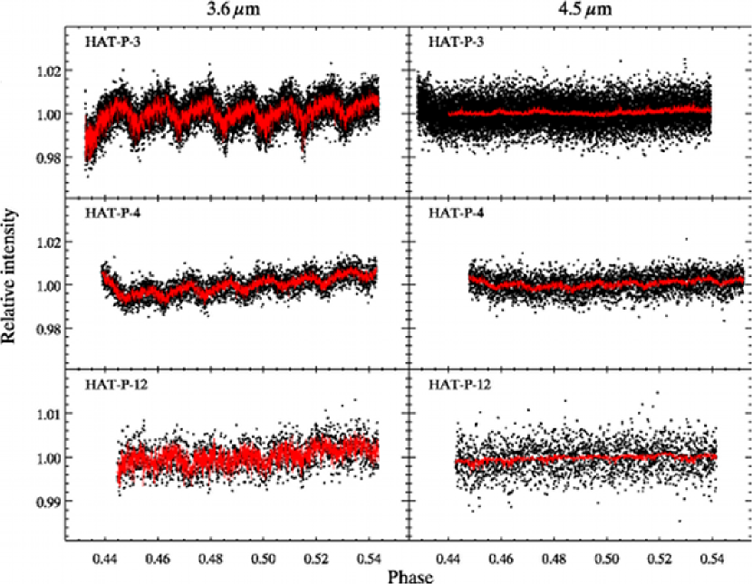
Figure 1.— The uncorrected time series photometry for HAT-P-3, HAT-P-4 and HAT-P-12 at 3.6 and 4.5 $\mu$m during secondary eclipse (dots), with the best fit eclipse model we obtain (red lines). These models include the astrophysical eclipse, and the instrumental effects: a linear ramp and the dependence of the measured intensity on the x and y-position of the stellar image on the detector. All photometric points are shown here, including the initial 49min of HAT-P-3 photometry, which we later reject. The best fit models only cover data that we have adopted for the fits. We discuss the data models in detail in Section 3.2. The HAT-P-12 photometry is shown on a smaller scale, since these data have the longest exposure time, and therefore the highest signal to noise per point. We do not detect the secondary eclipses of HAT-P-12b, and in these panels their depths are set to zero.

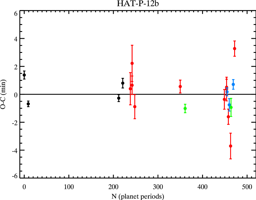
Figure 2.— The difference between the best fit transit times and the observed transit times for HAT-P-12b. The black symbols represent transit timings from the discovery paper for this planet (Hartman et al., 2009). Also included are timings from the Exoplanet Transit Database (ETD, http://var2.astro.cz/ETD/) compiled by Lee et al. (2012) (red symbols), and the measurements made by Lee et al. (2012) (blue) and Sada et al. (2012) (green). The horizontal axis shows the number of periods after the $\rm T_{0}$ transit. We do not see any obvious correlation in the residuals that may suggest a transit timing variation, and hence the presence of an additional companion in the system. On the other hand, the number of outliers on this plot may imply that the timing uncertainties in some of these studies are underestimated.

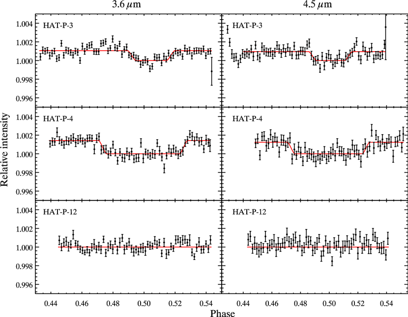
Figure 3.— The binned time series photometry for HAT-P-3, HAT-P-4 and HAT-P-12 at 3.6 and 4.5 $\mu$m during secondary eclipse after correction for instrumental effects (dots). The bin width is 0.0015 in units of orbital phase, corresponding to about 6 min 16 sec (HAP-P-3b), 6 min 36 sec (HAT-P-4b) and 6 min 56 sec (HAT-P-12b). The red lines represent the best fit eclipse model. The best fit coefficients were used to correct all data for instrumental effects, but we have only fitted to the data covered by the eclipse model. The HAT-P-12b eclipse depths have been set to zero in this plot.

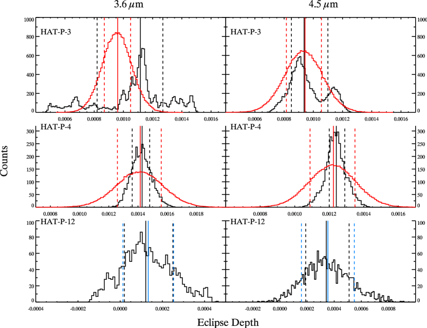
Figure 4.— We show the histograms of eclipse depth values that result from the prayer-bead technique (black) and the MCMC iterations (red). The vertical solid lines indicate the best values from the PBMC (black), MCMC (red) and linear regression (blue), which we take to be the median of the eclipse depth values of the prayer-bead and MCMC runs. The dashed lines bracket the regions centered on the medians that contain 68% of the recorded values for prayer-bead (black) and MCMC (red). Since MCMC and PBMC address different noise effects, we adopt as final best values and uncertainties the results from the technique which yields the larger uncertainty region. For HAT-P-12, since there is no secondary eclipse detected, the MCMC does not converge, and the prayer-bead is performed with the central phase fixed at 0.50007. The blue dashed lines indicate the $1\sigma$ estimates, based on the linear regression used to determine the eclipse depth in the original data sets. We conservatively adopt these as final best values since they are larger than the prayer-bead uncertainties.

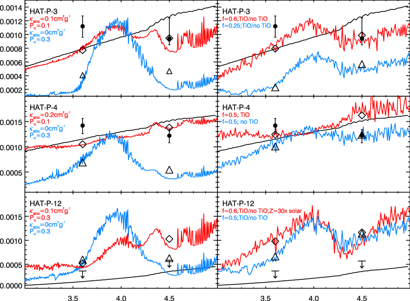
Figure 5.— The measured eclipse amplitudes as a function of wavelengths (filled circles) compared to different atmospheric models: a blackbody planet with a Kurucz model for the spectrum of the star (black lines Kurucz, 1979), Burrows planetary atmospheric models (left panels, Burrows et al., 2007, 2008), and similar atmospheric models by Fortney et al. (right panels, 2005, 2006a, 2006b, 2008). The downward arrows represent $3\sigma$ upper limits for the HAT-P-12b eclipse depths. We have assumed effective stellar temperatures for HAT-P-3 from Chan et al. (2011) and from Knutson et al. (2010) for HAT-P-4 and HAT-P-12. Left panels: The red lines represent the inverted models, with absorption coefficient of the unknown absorber in the upper atmosphere $\rm\kappa_{abs}=0.1,~{}0.2,~{}$and$~{}0.1$ $\rm cm^{2}\,g^{-1}$ and heat redistribution parameter $\rm P_{n}=0.1,~{}0.1,~{}$and$~{}0.3$ for HAT-P-3b, HAT-P-4b and HAT-P-12b, respectively. The blue lines are models with no inversion ($\rm\kappa_{abs}=0$ $\rm cm^{2}\,g^{-1}$) and $\rm P_{n}=0.3$ for all three planets. We over-plot the theoretical eclipse depths resulting from integrating the model stellar and planetary fluxes over the IRAC pass-bands (diamonds for the inverted models and triangles for the inverted ones). Right panels: In the Fortney model paradigm, where the stratospheric absorbers are assumed to be TiO and VO, HAT-P-3b and HAT-P-12b are sufficiently cool, so that the inverted and non-inverted (i.e., containing or not TiO and VO in the upper layers of the atmosphere) models are indistinguishable, due to TiO and VO condensation and rain-out. For HAT-P-3b, we show models with $f=0.6$ (red line) and $f=0.25$ (blue line); for HAT-P-4b, both models shown have $f=0.5$, but the red model has TiO in the upper layers of the atmosphere, while the blue one does not. For HAT-P-12b, the red line represents a model with $f=0.6$, while the blue line shows a model with $f=0.5$. All Fortney model atmospheres have solar composition, except the red model for HAT-P-12, which has metallicity 30 times higher than solar. For a more detailed explanation on the models see Section 4.1.

References

- Agol et al. (2010) Agol, E., Cowan, N. B., Knutson, H. A., Deming, D., Steffen, J. H., Henry, G. W., & Charbonneau, D. 2010, ApJ, 721, 1861
- Anderson et al. (2011) Anderson, D. R., Smith, A. M. S., Lanotte, A. A., et al. 2011, MNRAS, 416, 2108
- Ballard et al. (2010a) Ballard, S., Charbonneau, D., Deming, D., et al. 2010, PASP, 122, 1341
- Bean et al. (2006) Bean, J. L., Benedict, G. F., & Endl, M. 2006, ApJ, 653, L65
- Beerer et al. (2011) Beerer, I. M., et al. 2011, ApJ, 727, 23
- Burrows & Sharp (1999) Burrows, A., & Sharp, C. M. 1999, ApJ, 512, 843
- Burrows et al. (2007) Burrows, A., Hubeny, I., Budaj, J., Knutson, H. A., & Charbonneau, D. 2007, ApJ, 668, L171
- Burrows et al. (2008) Burrows, A., Budaj, J., & Hubeny, I. 2008, ApJ, 678, 1436
- Butler et al. (2004) Butler, R. P., Vogt, S. S., Marcy, G. W., et al. 2004, ApJ, 617, 580
- Campo et al. (2011) Campo, C. J., et al. 2011, ApJ, 727, 125
- Chan et al. (2011) Chan, T., Ingemyr, M., Winn, J. N., et al. 2011, AJ, 141, 179
- Charbonneau et al. (2005) Charbonneau, D., et al. 2005, ApJ, 626, 523
- Charbonneau et al. (2008) Charbonneau, D., Knutson, H. A., Barman, T., Allen, L. E., Mayor, M., Megeath, S. T., Queloz, D., & Udry, S. 2008, ApJ, 686, 1341
- Christiansen et al. (2010) Christiansen, J. L., et al. 2010, ApJ, 710, 97
- Cochran et al. (2011) Cochran, W. D., et al. 2011, ApJS, 197, 7
- Cooper & Showman (2005) Cooper, C. S. & Showman, A. P. 2005, ApJ, 629, L45
- Correia & Laskar (2010) Correia, A. C. M. & Laskar, J. 2010, in Exoplanets, ed. S. Seager, (Tucson: Univ. Arizona Press), 239
- Cowan & Agol (2011) Cowan, N. B., & Agol, E. 2011, ApJ, 729, 54
- Cowan et al. (2012) Cowan, N. B., Machalek, P., Croll, B., et al. 2012, ApJ, 747, 82
- Deming et al. (2005) Deming, D., Seager, S., Richardson, & L. J., Harrington, J. 2005, Nature, 434, 740
- Deming et al. (2011) Deming, D., et al. 2011, ApJ, 726, 95
- Demory et al. (2011) Demory, B.-O., et al. 2011, A&A, 533, A114
- Désert et al. (2011) Désert, J.-M., Charbonneau, D., Fortney, J. J., et al. 2011, ApJS, 197, 11
- Eastman et al. (2010) Eastman, J., Siverd, R. & Gaudi, B. S. 2010, PASP, 122, 935
- Fazio et al. (2004) Fazio, G. G., et al. 2004, ApJS, 154, 10
- Ford (2005) Ford, E. B. 2005, AJ, 129, 1706
- Ford (2006) Ford, E. B. 2006, ApJ, 642, 505
- Fortney et al. (2005) Fortney, J. J., Marley, M. S., Lodders, K., Saumon, D., & Freedman, R. S. 2005, ApJ, 627, L69
- Fortney et al. (2006a) Fortney, J. J., Saumon, D., Marley, M. S., Lodders, K., & Freedman, R. S. 2006a, ApJ, 642, 495
- Fortney et al. (2006b) Fortney, J. J., et al. 2006b, ApJ, 652, 746
- Fortney et al. (2008) Fortney, J. J., Lodders, K., Marley, M. S., & Freedman, R. S. 2008, ApJ, 678, 1419
- Fressin et al. (2010) Fressin, F., et al. 2010, ApJ, 711, 374
- Gillon et al. (2007a) Gillon, M., et al. 2007, A&A, 471, L51
- Gillon et al. (2007b) Gillon, M., Pont, F., Demory, B.-O., et al. 2007, A&A, 472, L13
- Grillmair et al. (2008) Grillmair, C. J., et al. 2008, Nature, 456, 767
- Hardin et al. (2012) Hardin, M., Harrington, J., Stevenson, K., et al. 2012, AAS/Division for Planetary Sciences Meeting Abstracts, 44, #200.09
- Harrington et al. (2007) Harrington, J., Luszcz, S., Seager, S., Deming, D., & Richardson, L. J. 2007, Nature, 447, 691
- Hartman et al. (2009) Hartman, J. D., Bakos, G. Á., Torres, G., et al. 2009, ApJ, 706, 785
- Hellier et al. (2010) Hellier, C., Anderson, D. R., Collier Cameron, A., et al. 2010, ApJ, 723, L60
- Hubeny et al. (2003) Hubeny, I., Burrows, A., & Sudarsky, D. 2003, ApJ, 594, 1011
- Knutson et al. (2007) Knutson, H. A, et al. 2007, Nature, 447, 183
- Knutson et al. (2008) Knutson, H. A., Charbonneau, D., Allen, L. E., Burrows, A., & Megeath, S. T. 2008, ApJ, 673, 526
- Knutson et al. (2009) Knutson, H. A., Charbonneau, D., Burrows, A., O’Donovan, F. T., & Mandushev, G. 2009, ApJ, 691, 866
- Knutson et al. (2010) Knutson, H. A., Howard, A. W., & Isaacson, H. 2010, ApJ, 720, 1569
- Knutson et al. (2012) Knutson, H. A., Lewis, N., Fortney, J. J., et al. 2012, ApJ, 754, 22
- Kovács et al. (2007) Kovács, G., Bakos, G. Á., Torres, G., et al. 2007, ApJ, 670, L41
- Kurucz (1979) Kurucz, R. L. 1979, ApJS, 40, 1
- Lee et al. (2012) Lee, J. W., Youn, J.-H., Kim, S.-L., Lee, C.-U., & Hinse, T. C. 2012, AJ, 143, 95
- Lewis et al. (2013) Lewis, N. K., Knutson, H. A., Showman, A. P., et al. 2013, ApJ, 766, 95
- Lodders & Fegley (2002) Lodders, K., & Fegley, B. 2002, Icarus, 155, 393
- Machalek et al. (2008) Machalek, P., et al. 2008, ApJ, 684, 1427
- Machalek et al. (2009) Machalek, P., McCullough, P. R., Burrows, A., Burke, C. J., Hora, J. L., & Johns-Krull, C. M. 2009, ApJ, 701, 514
- Maness et al. (2007) Maness, H. L., Marcy, G. W., Ford, E. B., et al. 2007, PASP, 119, 90
- Mighell (2005) Mighell, K. J. 2005, MNRAS, 361, 861
- Noyes et al. (1984) Noyes, R. W., Hartmann, L. W., Baliunas, S. L., Duncan, D. K., & Vaughan, A. H. 1984, ApJ, 279, 763
- Parmentier et al. (2013) Parmentier, V., Showman, A. P., & Lian, Y. 2013, A&A, submitted
- Perna et al. (2012) Perna, R., Heng, K., & Pont, F. 2012, ApJ, 751, 59
- Sada et al. (2012) Sada, P. V., Deming, D., Jennings, D. E., et al. 2012, PASP, 124, 212
- Sharp & Burrows (2007) Sharp, C. M., & Burrows, A. 2007, ApJS, 168, 140
- Southworth (2011) Southworth, J. 2011, MNRAS, 417, 2166
- Spiegel et al. (2009) Spiegel, D. S., Silverio, K. & Burrows, A. 2009, ApJ, 699, 1487
- Stevenson et al. (2010) Stevenson, K. B., et al. 2010, Nature, 464, 1161
- Stevenson et al. (2012) Stevenson, K. B., Harrington, J., Fortney, J. J., et al. 2012, ApJ, 754, 136
- Todorov et al. (2010) Todorov, K. O., Deming, D., Harrington, J., Stevenson, K. B., Bowman, W. C., Nymeyer, S., Fortney, J. J., & Bakos, G. A. 2010, ApJ, 708, 498
- Todorov et al. (2012) Todorov, K. O., Deming, D., Knutson, H. A., et al. 2012, ApJ, 746, 111
- Torres et al. (2007) Torres, G., Bakos, G. Á., Kovács, G., et al. 2007, ApJ, 666, L121
- Wright et al. (2011) Wright, J. T., Fakhouri, O., Marcy, G. W., et al. 2011, PASP, 123, 412
- Zahnle et al. (2009) Zahnle, K., Marley, M. S., Freedman, R. S., Lodders, K., & Fortney, J. J. 2009, ApJ, 701, L20