The Observed Squeezed Limit of Cosmological Three-Point Functions
Abstract
The squeezed limit of the three-point function of cosmological perturbations is a powerful discriminant of different models of the early Universe. We present a conceptually simple and complete framework to relate any primordial bispectrum in this limit to late time observables, such as the CMB temperature bispectrum and the scale-dependent halo bias. We employ a series of convenient coordinate transformations to capture the leading non-linear effects of cosmological perturbation theory on these observables. This makes crucial use of Fermi Normal Coordinates and their conformal generalization, which we introduce here and discuss in detail. As an example, we apply our formalism to standard slow-roll single-field inflation. We show explicitly that Maldacena’s results for the squeezed limits of the scalar bispectrum [proportional to in comoving gauge] and the tensor-scalar-scalar bispectrum lead to no deviations from a Gaussian universe, except for projection effects. In particular, the primordial contributions to the squeezed CMB bispectrum and scale dependent halo bias vanish, and there are no primordial “fossil” correlations between long-wavelength tensor perturbations and small-scale perturbations. The contributions to observed correlations are then only due to projection effects such as gravitational lensing and redshift perturbations.
I Introduction
In this paper we present a simple and complete framework to derive the late-time physical observables produced by the squeezed limit of primordial three-point functions, in particular those produced during inflation. These observables include the squeezed limit of the CMB bispectrum and the scale-dependent bias for large-scale structure tracers which crucially depends on the bispectrum in the squeezed limit Dalal et al. (2008); Matarrese and Verde (2008); Schmidt and Kamionkowski (2010). The main obstacle one encounters is the fact that, in order to calculate the bispectrum consistently, one has to work to second order in perturbation theory throughout. We show how this obstacle is overcome when one is interested in the squeezed limit. We take advantage of the fact that different sets of coordinates are convenient in different cosmological epochs and there is a careful choice that makes the computation easy and transparent. In the remainder of the introduction, we present a convenient way to choose coordinates by discussing the different steps that are summarized in Fig. 1.
A first step consists in computing the primordial correlators generated during the phase of primordial inflation. For this purpose, coordinates are used that are comoving with respect to some unperturbed universe (see e.g. Maldacena (2003)). A second step consists in describing the local late-time physical processes, such as for example the decoupling of photons during recombination or the formation of a dark matter halo, that lead to the generation of some light signal that eventually will reach the Earth. Since these processes take place in regions that are smaller in size than the curvature of the background metric (horizon scale ), they are best described in Fermi Normal Coordinates (FNC Manasse and Misner (1963)): this is the unique frame (up to three Euler angles) constructed along a timelike geodesic passing through a point in which the metric is Minkowski with corrections going as the spatial distance from the central geodesic squared. In an unperturbed FRW Universe, the corrections thus scale as , while in the presence of a metric perturbation the corrections involve second derivatives of (in particular, a constant or pure gradient metric perturbation is removed on all scales). The last step consists in relating the signals from the point of emission, for example the last scattering surface, or the position of a halo, to the observables measured on Earth, where scientists most naturally use FNC centered on the Earth’s world line.
|
|
|
|
|
|
|
In general, calculating the evolution of the bispectrum of perturbations in any coordinate frame including modes outside the horizon requires a full second-order relativistic calculation in cosmological perturbation theory, including gravity, baryon physics, radiation transfer, etc. This is in general a very complicated problem. However, a drastic simplification takes place when we limit ourselves to a particular configuration of the bispectrum in which two of the momenta, say and are much larger than the third, . This is often referred to as the squeezed limit with being the long mode and being the short modes.
Then, as described above, we can make use of the fact that in a expansion, the leading and next-to-leading order gravitational effects of the long-wavelength perturbation on the short modes can be removed by transforming to the local FNC frame, as was emphasized in Baldauf et al. (2011); Creminelli et al. (2012); Senatore and Zaldarriaga (2012a, b). The first non-trivial effect comes from the second spatial and time derivatives of the perturbation, which are suppressed by (see Sec. III for a more precise statement). We will ignore terms of this order in this paper, as they correspond to actual physical interactions, which will need to be treated in detail. However, up to this order, in the local FNC frame we can simply use linear theory. The non-Gaussian correlation will then be captured by averaging over an ensemble of FNC, each constructed to remove a different long mode.
In going from comoving coordinates to FNC, one subtlety arises from the fact that FNC are affected not only by perturbations but also by the expansion of the Universe. Because of this, no matter when the change of coordinates is performed, when using FNC we cannot avoid a period when the evolution at second order in perturbations becomes relevant. To see this, consider an expanding universe with a single long-wavelength perturbation, in addition to short-wavelength modes as in Fig. 2. The metric in standard FNC takes a simple flat space form only on scales smaller than the Hubble scale or the physical wavelength of the long mode , whichever is smaller. Therefore for the FNC metric to be valid in a region larger than the short modes, which is what we want to describe, we need ( being always true by assumption). But as soon as the short modes re-enter the horizon, , they start evolving, and acquire a non-trivial transfer function. In order to see that the evolution needs to be followed at non-linear order, consider our result for a general squeezed bispectrum Eq. (9). This expression contains terms involving the derivatives with respect to scale and time of the short mode power spectrum, which in general become non-trivial when and the short modes start evolving with time. It is clear that these terms cannot be accounted for by just multiplying each of the perturbations with the respective transfer function as linear perturbation theory would suggest.
A nice way out of this complication is to use conformal Fermi Normal Coordinates (), in which the metric is locally in the FLRW form, i.e. a homogeneous isotropic expanding Universe, rather than in the Minkowski form. These coordinates are valid up to a scale , where denotes the wavenumber of the long-wavelength perturbation considered. At late times, the small-wavelength modes are well inside the horizon and have in general been subject to non-linear evolution. Then, transforming from the frame to the usual FNC frame at a given spacetime point simply corresponds to a rescaling of the spatial coordinates.
The final step is to relate quantities defined in the local FNC frame (e.g. temperature of the gas, or halo mass) to the photons actually measured on Earth. This involves the photon propagation (“projection”) effects, such as lensing and redshift-space distortions Creminelli and Zaldarriaga (2004); Boubekeur et al. (2009); Creminelli et al. (2011a); Bartolo et al. (2012); Schmidt and Jeong (2012a); Lewis (2012). Here, we will adopt the “standard ruler” approach Schmidt and Jeong (2012a); Jeong and Schmidt (2013) since it conveniently encompasses all projection effects for various observables. Specifically, the derivation in Schmidt and Jeong (2012a) assumes that a ruler, such as a const contour, corresponds to a fixed physical spatial scale on a constant-proper-time hypersurface for a comoving observer, equivalent to a fixed spatial scale in FNC at emission.
Finally, at leading order, any physical (and necessarily non-gravitational) correlations between long-wavelength modes and small scale modes imprinted at early times and present in then simply add to these projection effects. The framework discussed above, which we summarize in Fig. 1, thus connects the bispectrum calculated in any convenient gauge during inflation with late-time observables such as the CMB bispectrum or the large-scale clustering of tracers. It can be applied to any model, and we will give some examples for single clock inflation and the “fossil” scenarios studied in Masui and Pen (2010); Giddings and Sloth (2011a, b); Jeong and Kamionkowski (2012). We should mention that the importance of in applications to the calculation of inflationary perturbations has been recognized and crucially used previously in the literature, e.g. in deriving various consistency relations Senatore and Zaldarriaga (2012b), in proving that is constant at large distances at all loop orders Senatore and Zaldarriaga (2012a) and in deriving the subleading corrections in to Maldacena’s consistency condition Creminelli et al. (2012). The issue of gauge artifacts in the squeezed limit of the bispectrum was also discussed in Tanaka and Urakawa (2011).
The outline of the paper is as follows: in Sec. II we derive some useful formulae to transform correlators from one set of coordinates to another. In Sec. III we introduce , and show how the squeezed-limit three-point correlations calculated in the standard way transform to this frame. In Sec. IV we derive how correlations in translate to observables, illustrating that, apart from projection effects such as lensing, the squeezed-limit three-point function in conformal Fermi coordinates is in fact the observed squeezed limit. In other words, if squeezed-limit correlations vanish in , then the observed squeezed limit is only due to projection effects. We conclude in Sec. V and leave some technical details to the appendices. App. A and App. B derive the transformation of the two and three point function in the squeezed limit, respectively, as one moves from one set of coordinates to another. In App. C we review the derivation of FNC and discuss their uniqueness in App. D.
II Transformation of small-scale correlations and the squeezed bispectrum
In this section we present some useful formulae to transform the two-point correlation function, Eq. (4), and three-point function and bispectrum in the squeezed limit, Eq. (9), from any one set of coordinates to another. The details of the derivation are left to appendix App. A and App. B.
Consider a scalar field , where denotes the spacetime position. We work in comoving coordinates throughout, so that is the conformal time. Under a general coordinate transformation , the field transforms as
| (1) |
Consider a patch on a const surface centered around the position . We would like to derive the correlation within that patch (defined with respect to the mean density over the patch) in terms of the two-point correlation function of in the unprimed coordinate system. Throughout the paper, we are considering the case where the coordinate transformation varies slowly over the spatial patch, that is where we can expand in terms of as
| (2) |
where , and
| (3) |
Note that and are functions of and . Here we have separated into a zeroth and first order piece (the sign is chosen so that maps to at linear order). The expansion to linear order in is sufficient, since we will only be interested in Fourier space contributions to the coordinate transformations up to order (see App. A). As shown in App. A, the correlation function of then becomes
| (4) |
The dependence on of the time shift Eq. (2) does not contribute at leading order.
We now turn to the squeezed limit of the three-point function , where denotes the fractional perturbation to (the results are identical when considering instead of ). This limit corresponds to the case where . Here, stands for any other field ( is not necessarily a scalar, but we suppress all tensor indices), such as for example density perturbations or tensor modes. Strictly speaking, is to be understood as coarse-grained on a scale . In the following, we will drop the primes on coordinates for clarity, since we will not employ the unprimed coordinates anymore. Further, we adopt the notation , that is, the long-wavelength (coarse-grained) field is not modified under the small-scale coordinate transformation within the patch. In the squeezed limit, the three-point function describes the modulation of the local two-point function at the location by the long-wavelength field evaluated at the distant point :
| (5) |
The precise location of the point in fact does not matter in the squeezed limit (as we prove in App. B), but we have chosen the midpoint as the most natural choice. We can now express in terms of the three-point function in unprimed coordinates and contributions from the transformation of small-scale correlations [Eq. (4)]. This yields
| (6) |
where denotes the cross-correlation between and . This expression gives the squeezed-limit three-point function of and (in the primed coordinates) in terms of derivatives of and the three-point function of and in the unprimed coordinate frame. As shown in App. B, we can derive an analogous expression in Fourier space, corresponding to the squeezed limit of the bispectrum:
| (7) |
As before, denote cross-power spectra between and , while denotes the power spectrum of . We can now further decompose as
| (8) |
where is the dimensionality of the space in which we define the correlations, and is traceless. Allowing , in particular will become useful when dealing with projected observables such as the CMB. We then obtain
| (9) |
Note that the contribution of the trace of scales as the logarithmic derivative of , while the trace-free component couples to the logarithmic derivative of itself. Instead of writing the bispectrum in terms of , one can also expand in , yielding zeroth order terms (with ) and first-order terms . The corresponding expression is given in App. B.
The results of this section are useful when, say, is easy to calculate, while is more readily related to observations. This will be the case we encounter below.
III Conformal Fermi Normal Coordinates
Our goal is to derive what the observable consequences are (as opposed to coordinate artifacts) of a given primordial bispectrum. For this purpose we follow the steps in Fig. 1, starting with conformal Fermi Normal Coordinates (). As we discussed in the introduction, if we want to avoid studying second order cosmological perturbation theory, it is not possible to directly connect the statistics of perturbations in the standard FNC frame of galaxies or the CMB (at the time when the photons we observe were emitted) with the statistics calculated when all perturbations are superhorizon. The reason is that the perturbative corrections to the Fermi frame metric are of order , where are the physical FNC coordinates, so that the metric in FNC is not approximately flat on the scales of superhorizon perturbations. On the other hand, if we were to move from the global coordinates to FNC at a later time when the short wavelength modes have long re-entered the horizon, we would have to take into account their evolution after horizon entry at second order in the global coordinates.
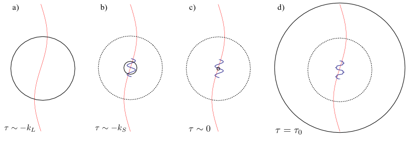
To overcome this obstacle, in this section we introduce a new coordinate frame which is valid throughout inflation and the hot big bang era (assuming nothing dramatic happens to superhorizon perturbations during this time), and further connects easily with the FNC frame at late times. This provides a well-defined framework for studying observables related to primordial non-Gaussianities in the squeezed limit. To visualize the advantage of , consider Fig. 2. Each one of the four panels shows the Hubble scale (solid circle) and the region of validity of the (dashed line) at a different moment in time. The long (red line) and short (blue line) modes are also shown for comparison. One can immediately appreciate the fact that from very early time when the long mode is still inside (or about to leave) the horizon all the way until late time when the long mode has re-entered the horizon, the region of validity of amply encompasses the short modes. This is in contrast with standard for which the presence of the Hubble scale makes this impossible. The primordial correlators, typically computed in comoving coordinates, take a simple form once both the short and long modes have left the horizon and cease to evolve. Any time after that moment and before the small-scale modes reenter the horizon constitutes a good time to transform from global conformal coordinates to .
Let us assume we are given the primordial correlations during inflation in some gauge, where the metric is written as
| (10) |
Here we have denoted the conformal metric with a bar. In the absence of perturbations, and . We will work up to linear order in metric perturbations.
As in the usual Fermi normal coordinate construction, we consider a central timelike geodesic of a comoving observer. However, instead of constructing the FNC with respect to , we construct conformal Fermi normal coordinates () with respect to . That is, within a region around the central geodesic, the metric in these coordinates is approximately . The corrections to this metric, which determine the size of this region which we will call “ patch”, are given by second derivatives of the metric perturbations. Correspondingly, the size of the patch is linked to the wavelength of the metric perturbations considered. In the following, we will be interested in (long-wavelength) perturbations with wavenumber , so that the size of the patch is of order .
The transformation from coordinates to , for a patch centered at the spatial origin at time is given by (see App. C.2)
| (11) | ||||
| (12) |
The inverse of this transformation is at linear order
| (13) | ||||
The metric in then becomes
| (14) | ||||
Here, , , and primes denote derivatives with respect to , while spatial derivatives are with respect to . The linear and quadratic coefficients in the coordinate transform Eq. (12) are uniquely determined by the requirement that the lowest order contribution to is order . However, given that the quadratic corrections are determined by the cubic order terms in the coordinate transformation, one might wonder whether the quadratic corrections to are unique. One can show (see App. D) that and are indeed unique. However, there is freedom to change the quadratic term in if one allows the spatial coordinate lines to be non-geodesic at order .
In summary,
| (15) |
Let us disregard the corrections for the moment. The remaining corrections to the conformal Fermi frame metric scale as second derivatives of the metric perturbation multiplied by the spatial coordinate squared. Thus, instead of being order as the usual FNC corrections , they are of order , where is the comoving wavenumber of the perturbation (in slight abuse of notation, we drop the bar over since we will only be dealing with comoving Fourier wavenumbers). Within the patch of size , we can remove the effects of the long-mode perturbation (in comoving coordinates) at all times — through horizon exit and reentry.
This very useful result only holds if are of order or smaller, which is the case for all models of single field inflation in which the background is an attractor solution. In principle one can engineer a model in which, for a short period of time, the background is not close to an attractor solution, but rather it is evolving towards one. In this case, the superhorizon modes can have, for a short period of time, sizable time derivatives Namjoo et al. (2013); Chen et al. (2013). For example, if is larger than , corresponding to significant superhorizon evolution of the spatial metric perturbation, then we cannot follow the conformal Fermi frame through the entire duration of inflation. In case the evolving part of is isotropic (or can be made so by a suitable change of coordinates),
| (16) |
where denotes the origin in comoving coordinates around which we construct the frame, then we can absorb its effect into a modified scale factor,
| (17) |
In a modified frame constructed with the scale factor the rapidly evolving part now disappears. We thus see that in this case, a long-wavelength metric perturbation does not simply shift the time and rescale spatial coordinates, but rather corresponds to a change in the entire background cosmology. This is possible only because the original “unperturbed” background cosmology, namely , was unstable (i.e. not an attractor). Given that the generation of small-scale perturbations depends on the background cosmology, we in general expect a non-trivial coupling between very long wavelength metric perturbations and small-scale modes in this case. If is not isotropic, then we cannot absorb its effect into a modified scale factor. Instead, the different spatial coordinates are rescaled differently, leading to an anisotropically expanding Universe of Bianchi I type.
Similar arguments apply to the case where is larger than . Here the lowest order effect will be a Bianchi I-type Universe, since isotropy is necessarily violated.
III.1 Bispectra in global and coordinates
Let us assume that we can calculate the statistics of a scalar field in the global coordinates Eq. (10). Specifically, we consider fluctuations at a given epoch during inflation, typically evaluated right after horizon crossing. For simplicity, we will restrict to a scalar field, although the extension to other spins is straightforward. Given the results from Sec. II and the coordinate transform Eqs. (12)–(13), we can then immediately derive the transformation of the two-point correlation measured in a patch around position at conformal time from the global coordinates to the frame. Note that if is non-Gaussian, then the correlation function measured in a given patch will correlate with long-wavelength perturbations.
In the present case, the primed coordinate system of Sec. II is , while denote the global coordinates in the gauge chosen. We can then read off and from Eq. (13):
| (18) | ||||
| (19) |
With this, Eq. (4) yields
| (20) | ||||
where denotes the correlation function of in the local frame. Now consider the bispectrum , where is any perturbation. The results from Sec. II immediately show how this bispectrum transforms into . Denoting quantities as , we obtain
| (21) |
where all correlations on the r.h.s. are evaluated at . Here is the trace of the spatial metric perturbation while is the trace-free part. The significance of this result will become clear in the application to single-field inflation which we will consider next.
III.2 Single-field inflation in comoving gauge
In the following, we restrict to comoving gauge. In the notation of Maldacena (2003), we have
| (22) |
where is tranverse-traceless and contains the tensor perturbations. For the attractor solution of single-field inflation, the constraint equations in this gauge yield Maldacena (2003)
| (23) |
To order , we can thus neglect the contribution from the time shift . Note that this is merely a consequence of the particular gauge chosen. The only remaining contribution to the transformation of the bispectrum [Eq. (21)] then comes from and the tensors . For the scalar contribution, which we indicate with and “S” over the equal sign, we obtain
| (24) |
where throughout . We are in particular interested in the bispectrum of the curvature perturbation , i.e. . Since is not a scalar, our derivation in Sec. II does not strictly apply. However, it is straightforward to show that for the purposes of this transformation, the small-scale modes behave as a scalar. Recall that only the spatial transformation is relevant at the order we are interested. The comoving gauge condition, where is the inflaton perturbation is thus still satisfied in the frame. Further, the spatial components of the metric transform as
| (25) |
We now write , separating into long- and short-wavelength pieces on the scale of the patch within which the correlation function is measured. Then, the transformation to removes up to second derivatives, while is not affected since it does not contain any long-wavelength components. We thus obtain
| (26) |
Thus, the short-wavelength perturbations transform effectively as a scalar [Eq. (1)]. We obtain for the bispectrum of curvature perturbations in the frame:
| (27) |
where is the three-point function calculated in comoving gauge. As shown in Maldacena (2003); Creminelli et al. (2011b), this is in the squeezed limit given by
| (28) |
where is defined through . Eq. (28) is usually referred to as the consistency relation. We now see that the first term in Eq. (27) exactly cancels the contribution from , leading to
| (29) |
We thus conclude that in single-field inflation, the bispectrum in the squeezed limit is zero in the conformal Fermi frame, with corrections going as .
The case for non-scalar metric perturbations follows analogously. Decomposing the long-wavelength metric perturbation into polarization states,
| (30) |
we obtain (the “T” over the equal sign now stands for tensor)
| (31) |
Assuming that the different polarization states are statistically independent, we obtain for the tensor-scalar-scalar bispectrum [again using the transformation property Eq. (26)]
| (32) |
The squeezed-limit bispectrum in comoving gauge was also derived in Maldacena (2003):
| (33) |
We again see that the two terms in Eq. (32) cancel in single-field inflationary models. Thus, in single-field inflation, the tensor-scalar-scalar bispectrum vanishes in the squeezed limit in , so that there are no correlations between long-wavelength tensor modes and small-scale fluctuations in this frame. The lowest correction are again of order .
We can phrase the main result of this section as follows: at leading order, the squeezed-limit three-point correlations in single-field inflation, which obey the “consistency relation”, are equivalent to the statement that there is no correlation between infinitely long and short wavelength modes in the conformal Fermi frame, specifically,
| (34) |
where stands for any component of , and .
Since this latter is a physical, gauge-invariant statement, it is expected to hold not only at leading order in spacetime perturbations but at higher orders as well. The FNC approach can also help elucidate why there is no such correlation up to order in single field models. One might wonder why such a correlation cannot be imprinted at early times when the long wavelength perturbation was inside the horizon, . Far inside the horizon, we can neglect gravity and are essentially dealing with a scalar field in vacuum which adiabatically tracks the slowly evolving background, and a given mode is only excited once its wavelength becomes of order the horizon. Contributions to correlations from within the horizon are exponentially suppressed Senatore and Zaldarriaga (2012a, b) (see also Flauger et al. (2013)). On the other hand, when , the long-wavelength mode is far outside the horizon and its effects can be removed by a coordinate transformation up to order .
IV Connection to late-time observations
As explained in Sec. III, we can follow the patch all the way through the end of inflation and horizon re-entry of both long and short modes, provided that perturbations do not evolve significantly when they are outside the horizon. In this section, we show how the squeezed-limit correlations in the frame can be related to observations made from Earth today.
Let us assume we observe correlations of some field at late times, i.e. at or after recombination. In linear theory, assuming adiabatic initial conditions, we can relate to the curvature perturbation through some transfer function ,
| (35) |
For matter density perturbations, is defined in Eq. (73) below. Similarly, we assume the long-wavelength perturbation is evolved with some transfer function,
| (36) |
where we have assumed the limit (the lowest order dependence of will be ; of course, will differ for scalar and tensor perturbations). As long as superhorizon perturbations evolve slowly (in the sense that are smaller than or of order ), the conformal Fermi coordinate patch, i.e. the region over which corrections to the metric are small, is essentially constant in (comoving) size throughout horizon exit and reentry of the short-wavelength modes. As we have seen, this applies in particular to single-field inflation models. Thus, at the conformal time at which the photons we observe today were emitted, the metric in is
| (37) |
If we transform coordinates through
| (38) |
the metric in the coordinates becomes
| (39) |
In other words, are the usual Fermi coordinates (FNC) defined around the same timelike geodesic as the . Depending on whether the long-wavelength modes for which we constructed the patch have entered the horizon, either the order or the order corrections will be dominant; however, this is not relevant for the discussion that follows. Eq. (38) corresponds to a rescaling of the time coordinate, leaving the timelike unit vector and const hypersurfaces unchanged, and a time-dependent rescaling of the spatial coordinates. Since the spatial rescaling is the same everywhere on a const hypersurface, this implies that, for models that obey the consistency condition, Eq. (34) is still valid at late times in the FNC frame:
| (40) |
where denote perturbations in the FNC frame. Recall that the squeezed limit of three-point functions corresponds to the modulation of local two-point functions by long-wavelength perturbations. Thus, another way of phrasing this result is that a surface of constant correlation in the frame, const, defines a standard ruler—a fixed spatial scale—as considered in Schmidt and Jeong (2012a), with corrections proportional to second derivatives of only. Hence, in standard single-field inflation and any other case where Eq. (34) holds, the ruler scale is statistically the same everywhere on a const hypersurface, and there is no correlation with long-wavelength perturbations.
The apparent correlations induced between long-wavelength modes and small-scale correlations are then given by the ruler perturbations derived in Schmidt and Jeong (2012a). We can use their results together with Sec. II to derive these contributions to observed squeezed-limit three-point functions, and make the connection with known results.
In general, there are two effects modifying the observed two-point correlation within a given patch. First, there is the transformation from the local FNC to the observed comoving coordinates , which are inferred from the observed position of the source in the sky and its redshift through , , where is the comoving distance-redshift relation in the background (in case of the CMB, this is slightly modified, as we will discuss in Sec. IV.1). Let us assume we observe a scalar field (whose perturbation is ). Then, as described in Sec. II, is given in terms of the field in the Fermi frame as
| (41) |
At fixed observed redshift, we can write the transformation from to as
| (42) |
Here , is the perturbation in proper time from a constant observed redshift surface Jeong and Schmidt (2013), and can be seen as the generalization to three dimensions of the magnification matrix. Note that and are gauge-invariant. Specifically, using the notation of Schmidt and Jeong (2012a), is given by
| (43) |
where is the projection operator perpendicular to the line of sight. and are the gauge-invariant ruler perturbations derived in terms of the metric perturbations in Schmidt and Jeong (2012a). For example, the transverse matrix contains the magnification and shear.
The second effect is a rescaling of the observed field by projection effects. If there are multiplicative projection effects, then we have
| (44) |
Here we think of as averaged over the patch within which we measure the correlation function of small-scale perturbations. For example, in case is the number density of some tracer, then projection effects such as gravitational lensing modify the physical volume that corresponds to a fixed region in the observed coordinates , thus rescaling the number density. Gravitational redshift and ISW effect lead to an analogous rescaling in case of the CMB. The factor also rescales the fluctuations in within the region considered, and correspondingly rescales the correlation function by , leading to
| (45) |
where we have used Eq. (4) in the second line. Straightforward application of the results of Sec. II then yields the bispectrum of the observed density perturbation in the squeezed limit, in terms of the projection effects and the bispectrum of in the frame:
| (46) |
where . The bispectrum of a two-dimensional projected field (in the flat-sky limit) correspondingly becomes
| (47) |
where again .
The bispectrum in FNC frame is equivalent up to transfer functions (and radial projection, in the 2D case) to the bispectrum in , which as we have seen vanishes in the squeezed limit for single-field inflation. In this case, the terms due to “projection effects” are the only remaining contributions.
In the following we present two applications of Eqs. (46)–(47): the CMB bispectrum in the squeezed limit, and the scale-dependent non-Gaussian halo bias.
IV.1 CMB bispectrum
In this section, we illustrate the main result of the previous section on the observed squeezed-limit bispectrum, Eq. (47), with the CMB. We will make direct connection with the results of Creminelli et al. (2011a); Bartolo et al. (2012). A more sophisticated and accurate treatment which is based on an closely related approach has been presented in Lewis (2012).
We assume single-field inflation so that the frame contribution vanishes. We will adopt the conformal-Newtonian gauge in this section,
| (48) |
although it is straightforward to derive the results in a general gauge.
The observed CMB photons originate from the last scattering surface, which occurred at a fixed physical age of the Universe, that is, at constant proper time for the comoving primordial plasma. The proper time of a comoving source passing through at coordinate time is given in the metric convention Eq. (48) by
| (49) |
where and are the physical-time – conformal time relations in the background.
The value of is obtained by combining atomic physics with the mean observed temperature of the CMB today. The CMB temperature perturbations on scales that were super-horizon at recombination () originate entirely from projection effects; in other words, the large-scale CMB temperature perturbations can be seen as a special case of the evolving ruler described in Jeong and Schmidt (2013). Essentially, the standard ruler is in this case given by the photon occupation number . In fact, since lensing conserves surface brightness, the only contribution to the fractional CMB temperature perturbation is the redshift perturbation on a fixed proper time surface, which is equivalent to minus the quantity defined in Jeong and Schmidt (2013):
| (50) |
where have used that for a free-streaming blackbody. As shown in Jeong and Schmidt (2013), this immediately yields the CMB temperature perturbation in the gauge Eq. (48) as
| (51) | ||||
| (52) |
In the second line, we have assumed that the relevant perturbations are superhorizon, const (since we are interested in where the acoustic contributions can be neglected), and that recombination happened long after matter-radiation equality so that .
IV.1.1 Transforming from to observer coordinates
As we have seen, the CMB temperature on large scales is modified by the temperature perturbation Eq. (51), which is entirely due to the effects on photons as they propagate from the last scattering surface to the observer. Thus, the CMB temperature that would be measured in the local Fermi frame at emission is rescaled by in the observer frame, so that in the notation of Sec. IV, .
The second ingredient is the coordinate transformation from to the observer frame. Projected onto the sky, the matrix becomes the usual weak lensing distortion tensor , which we can write to linear order as
| (55) |
In particular, . The magnification (a gauge-invariant quantity) is easily adapted from the results of Schmidt and Jeong (2012a). The key difference is the meaning of the perturbation to the logarithm of the scale factor at emission, which here we call . By definition,
| (56) |
Whereas the quantity of Schmidt and Jeong (2012a) is derived for photons arriving with a fixed observed redshift, in the present case we need the corresponding expression for a constant proper time at emission. This is easily derived from the expression for the proper time Eq. (49). Requiring and solving for yields
| (57) |
which leads to
| (58) |
so that
| (59) |
We now use this result in the general-gauge expression Eq. (51) of Schmidt and Jeong (2012a),
| (60) |
In Eq. (60), is the coordinate convergence, i.e. the transverse (with respect to the line of sight) divergence of the transverse displacements, and is the displacement along the line of sight. In the metric Eq. (48) we have Schmidt and Jeong (2012a)
| (61) | ||||
| (62) | ||||
| (63) |
where , and we have made the same assumptions about superhorizon perturbations and matter domination as in Eq. (51). The magnification then becomes
| (64) |
Here we have used that during matter domination.
Using the relation between convergence and shear in -space, we then have in the flat-sky approximation
| (65) | ||||
| (66) |
In Eq. (65), we have approximated as the CMB temperature power spectrum without ISW contribution, and neglected the contribution from the line-of-sight displacement . The latter is small due to cancelation along the line of sight except for the very smallest for the time delay [first term in Eq. (62)], and suppression by in case of the second term of Eq. (62) (the third term in Eq. (62) only contributes to the monopole). See Lewis (2012) for a quantitative evaluation of these contributions. Finally, for the contribution from the time shift, since . However, the CMB power spectrum observed today only evolves on the Hubble scale today, so that
| (67) |
Thus, this contribution is suppressed by with respect to the leading contributions, and we will neglect it in what follows.
IV.1.2 Squeezed-limit CMB bispectrum
Inserting these results into Eq. (47) then yields
| (68) |
where , and . Apart from the very small contribution from , this is an exact result for the squeezed-limit CMB bispectrum as long as the approximation of the Sachs-Wolfe limit is accurate for modes of wavenumber (). Note that no such assumption has been made about the short-wavelength modes . The cross-correlation between CMB temperature and can further be decomposed as
| (69) |
i.e. an early-time correlation with the potential , and a late-time correlation between and the ISW contribution. The latter contribution has recently been detected by the Planck satellite Planck Collaboration et al. (2013).
In order to compare with Creminelli et al. (2011a); Bartolo et al. (2012), we neglect the ISW-lensing correlation, and use the result of Boubekeur et al. (2009) for early-time correlations in the Sachs-Wolfe regime,
| (70) |
Further, we neglect the distinction between and . We then have
| (71) |
This agrees with the final result of Creminelli et al. (2011a), while it differs from Bartolo et al. (2012) because a subset of the lensing contributions was neglected there.
One can show (App. C of Schmidt and Jeong (2012a)) that the contribution of metric perturbations with wavenumber to the CMB temperature as well as the ruler perturbations scale as in the limit . The contributions in the low- limit can be interpreted as the lowest order corrections to our local conformal Fermi patch. Unless there is some physical coupling between currently superhorizon and subhorizon modes Schmidt and Hui (2012), the observable imprint of any superhorizon perturbation (scalar or tensor) is suppressed by .
IV.2 Non-Gaussian halo bias
For Gaussian initial conditions, the distribution of large-scale structure tracers (such as galaxies, clusters, etc.) in the large-scale limit follows the distribution of matter. More accurately, this holds on a constant proper time slice Baldauf et al. (2011); Schmidt et al. (2012). While the abundance of tracers depends on the amplitude and shape of local small-scale fluctuations, in the Gaussian case these are statistically the same everywhere. That is, at fixed proper time in their respective FNC frame, all observers see statistically the same small-scale fluctuations. These then do not contribute to correlations in the tracer abundance on large scales. Non-Gaussianity in the primordial perturbations can however couple small-scale fluctuations to large-scale perturbations. As we discussed in Sec. II, this in fact precisely corresponds to the squeezed limit of (at lowest order) the three-point function. Thus, neglecting for the time being any projection effects in going from the FNC frame to the observed positions and redshifts of tracers, there is a non-Gaussian scale-dependent bias if and only if the amplitude of small-scale fluctuations in the FNC frame correlates with long-wavelength perturbations—that is, if there is a non-zero squeezed-limit bispectrum , where denotes the matter density perturbation in the FNC frame.
Using Eqs. (35)–(36), the bispectrum of is related to the bispectrum of curvature perturbations in the frame through
| (72) |
where
| (73) |
is the relation in Fourier space between the density and the curvature perturbation, is the matter transfer function normalized to unity as , and is the linear growth rate of the gravitational potential normalized to unity during the matter dominated epoch.
In order to derive the scale-dependent bias, we now assume that the tracer abundance is mostly sensitive to the variance of the density field on a scale , typically chosen to correspond to the Lagrangian scale of the tracer. See Schmidt et al. (2012); Schmidt (2013a) for a more general and detailed discussion. The contribution to the tracer two-point function is then proportional to , where denotes the FNC-frame density field smoothed on scale . As shown in, e.g. Desjacques et al. (2011); Scoccimarro et al. (2012), the large-scale scale-dependent bias is then given by
| (74) |
where is the filter function in Fourier space, and we have dropped the arguments for brevity. As long as is much less than the typical values of in the integrand (), the bispectrum here is evaluated in the squeezed limit Schmidt (2013b). Let us perform a leading order expansion in this limit,
where is as defined before. Here, we have assumed a scale-invariant bispectrum (otherwise, the coefficients are in general functions of ), and no dependence on the angle between and as is typically the case (but see Endlich et al. (2012) for a counterexample). The lowest order piece leads to a scale dependence of
| (75) |
which corresponds to the usual scale-dependent bias from local non-Gaussianity. The second part leads to a scale-dependence of
| (76) |
which is much weaker and only relevant on scales where the transfer function departs from unity. Since in single field inflation [Eq. (34)], we conclude there is no scale-dependent bias induced on scales in these models.
The scale-dependent bias discussed here refers to the FNC frame of the tracers; there are contributions to the observed scale-dependent bias from projection effects, i.e. from transforming from the tracer FNC frame to observed positions and redshifts (in our own FNC frame). Those have been derived in Yoo et al. (2009); Challinor and Lewis (2011); Bonvin and Durrer (2011); Baldauf et al. (2011); Jeong et al. (2012), but are generally quite small. Matching to the scale-dependent bias from local non-Gaussianity, they correspond to for a wide range of tracer parameters Jeong et al. (2012).
V Conclusions
In this work we have presented a simple and complete framework to translate the squeezed limit of any primordial three-point function into observables such as the squeezed limit of the CMB temperature bispectrum and the scale-dependent halo bias. In Fig. 1 we have spelled out the various steps of the computation and the respective choices of gauge. The different gauges have been chosen in such a way that the whole computation from horizon exit during inflation until observation on earth can be performed using only linear perturbation theory. This required the introduction of a conformal version of the well known Fermi Normal Coordinates (used in Senatore and Zaldarriaga (2012a, b) for inflationary correlators), in which the spacetime is locally FLRW as opposed to Minkowski. As an example we have applied our formalism to standard single-field slow-roll inflation. We have shown that Maldacena’s consistency condition Maldacena (2003) in the squeezed limit of the scalar bispectrum implies that the signal in the CMB bispectrum and halo bias vanishes exactly. Although this result was already known, our approach provides a simple, concise and physically clear derivation. This calculation can straightforwardly be generalized to higher N-point functions in the squeezed limit.
In addition, our approach sheds light on the proposal that there are observable correlations between long wavelength tensor modes and short wavelength scalar perturbations Masui and Pen (2010); Giddings and Sloth (2011a, b) (see also Jeong and Kamionkowski (2012)). These authors state that the correlation vanishes as long as the long tensor mode is outside of the Hubble radius . This can be understood using the results of our section Sec. III, where we show that a constant and a pure gradient mode of the metric are absorbed by the change of coordinates when going to the Fermi Normal frame. The physical effects of a long mode that a local observer can measure are hence suppressed at least by and are therefore small for superhorizon perturbations. Notice in particular that the standard result for the tensor-scalar-scalar bispectrum in single field inflation Maldacena (2003) is just a restatement of this fact but using comoving coordinates. In these coordinates the tensor-scalar-scalar bispectrum takes exactly the right form such that, changing to Fermi Normal coordinates, one finds vanishing correlation up to corrections of order as we saw in Sec. III.2. After the tensor mode enters the horizon, it starts oscillating and decays. During the epoch around horizon crossing, , the tensor mode can induce some tidal effects on the short scale scalar power spectrum (see Schmidt and Jeong (2012b) for an evaluation of this effect for the shear). We did not compute this effect here, and leave this interesting possibility for future work. Further, as discussed in Sec. IV, there are projection (photon propagation) effects induced by the long-wavelength tensor mode Kaiser and Jaffe (1997); Dodelson et al. (2003); Schmidt and Jeong (2012b). However, these are again suppressed by in the limit. In summary, just as for the scalar bispectrum, a detection of a squeezed-limit tensor-scalar-scalar bispectrum through the measurements described in Masui and Pen (2010); Jeong and Kamionkowski (2012), at a level larger than expected from tidal and projection effects, would rule out single-field inflation.
The framework we have developed in this paper is also useful in other classes of models that have not yet been directly related to observations. One example is resonant non-Gaussianity Chen et al. (2007, 2008); Flauger and Pajer (2011); Leblond and Pajer (2011); Hannestad et al. (2010), which is a generic prediction of many models of axion inflation (see Pajer and Peloso (2013) and references therein), in particular inflation from axion monodromy McAllister et al. (2010); Flauger et al. (2010); Berg et al. (2010). In these models the inflationary potential has sinusoidal modulations, which lead to oscillations in the time evolution of the background. Since these oscillations average to zero over a period, they can give corrections to the slow-roll parameter that are larger than is usually allowed and nevertheless be perfectly compatible with current power spectrum data (see e.g. Flauger et al. (2010); Aich et al. (2013); Peiris et al. (2013)). The resonant bispectrum satisfies Maldacena’s consistency condition Flauger and Pajer (2011); Creminelli et al. (2011), but because of oscillations the amplitude of the primordial bispectrum in the squeezed limit is not suppressed by small slow-roll corrections. In light of this, one might wonder whether these models lead to some detectable signal in the scale dependent halo bias. Cyr-Racine and Schmidt (2011) showed that indeed resonant non-Gaussianity produces oscillations in the mass dependence of the non-Gaussian halo bias, which is a very unique signature. However, the leading contribution in the large-scale limit to the effect derived in that paper is only a coordinate artefact as shown here. While the halo bias thus has to asymptote to a scale-independent value in the large-scale limit, we expect some interesting effects on intermediate scales. To compute the actual size of this effect it is important to re-write the primordial resonant bispectrum in terms of FNC. It would be very interesting to perform this analysis using the framework constructed in this paper. There are also other models of the early universe (both inflationary and not) in which the metric perturbations do not freeze outside of the horizon. For example, it has been argued in Namjoo et al. (2013); Chen et al. (2013) (see also Kinney (2005)) that this allows one to violate Maldacena’s consistency condition. Another interesting model with a peculiar behavior in the squeezed limit is Khronon inflation, studied in Creminelli et al. (2012). It would be interesting to use our approach to derive the observational prediction of these and similar models.
On the other hand, multifield inflationary models in general feature a non-trivial bispectrum in the squeezed limit. In this case, curvature perturbations evolve outside the horizon, and the small-scale fluctuations are sensitive to their presence as they essentially evolve in a different FRW background (or, more generally, in a homogeneous anisotropic Universe). This reasoning can be used to connect the squeezed-limit correlators in multifield inflation to late-time observables in a similar way as outlined here for single-field inflation.
Acknowledgments
We acknowledge useful discussions with Liang Dai, Raphael Flauger, Steven Giddings, Donghui Jeong, Marc Kamionkowski, Justin Khoury, Kiyoshi Masui, Ue-Li Pen, and Martin Sloth. E. P. is supported in part by the Department of Energy grant DE-FG02-91ER-40671. F. S. is supported by NASA through Einstein Postdoctoral Fellowship grant number PF2-130100 awarded by the Chandra X-ray Center, which is operated by the Smithsonian Astrophysical Observatory for NASA under contract NAS8-03060. M. Z. is supported in part by the National Science Foundation grants PHY-0855425, AST-0907969, PHY-1213563 and by the David & Lucile Packard foundation.
Appendix A Coordinate transformation of two-point correlations
Consider a scalar field . Under a general coordinate transformation , transforms as
| (77) |
We define the unequal-time two-point correlation of , measured within a patch through
| (78) |
where a subscript indicates an average over the patch, and we have defined , so that by construction the average over the patch of vanishes. The correlation function introduced above is then defined as
| (79) |
We will consider an alternative definition, the correlation function of , below and show that it transforms in the same way. Further, we will denote the equal time correlation function as in the following for simplicity.
Now let us consider the equal-time two-point correlation for , measured in the same patch:
| (80) |
where , and we have defined for convenience , and analogously for . By assumption, the coordinate transform is slowly varying over the patch. We then Taylor expand the coordinate transformations around the center point ,
| (81) |
where , and . We will discuss below why going to linear order in is sufficient. We then have
| (82) |
since is symmetric in and . Thus, at linear order in , the equal time correlator in primed coordinates is an equal time correlator in unprimed coordinates. We thus have
| (83) |
We now define the correlation function of in the same way as that for [Eq. (78)], which yields
| (84) |
where
| (85) |
The second equality again holds to linear order in , at which order the average of over the patch at fixed is just . We will discuss this definition of in App. A.1 below. Thus, the first term in each of Eqs. (83)–(84) agrees, and hence so must the second term:
| (86) |
We can similarly derive what happens to , which is the correlation function defined in terms of . In this case, we have
| (87) |
For , this yields
| (88) |
Now we define the correlation function of in the same way as that for [Eq. (78)], which yields
| (89) |
Thus, we see that transforms in the same way as , namely
| (90) |
There are thus two ways in which the general affine coordinate transform affects the correlation function in primed coordinates: first, there is the spatial transformation of the separation vector, ; second, the primed correlation function is evaluated at a different point in space and time (here, we have only made the time shift explicit in the notation, but note that the corrrelation function on the right hand side is to be evaluated within a patch centered on ).
The linear order expansion in Eq. (81) neglects higher derivative terms in the coordinate transformation, i.e. it is valid in the limit that the transformation is slowly varying over the patch. The terms we are neglecting in Eq. (81) correspond to terms of order and higher, where is the wavenumber of the long-wavelength mode that contributes to the coordinate transformation. Since we are neglecting terms of order throughout this paper, it is sufficient to expand to linear order.
A second simplification occurs because we are only considering three-point correlations in this paper. In this case, it is sufficient to consider the linear response of to the coordinate transformation. We thus write
| (91) |
and work to linear order in and . Further, we can neglect the effect of the spatial shift in the position at which is evaluated. This is because the contribution from this shift,
| (92) |
is second order, since both the spatial shift and the location dependence of are at least linear order in the long-wavelength perturbations. Eq. (86) then simplifies to Eq. (4),
| (93) |
A.1 Coordinate transformations in the presence of non-trivial backgrounds
There is a conceptual point to clarify about the transformation properties of perturbations under changes of coordinates. There are two different but equivalent ways to work with coordinate transformations when studying perturbations on top of some non-trivial background. The first one consists in changing every field in the same way, whether it is going to be treated as a background or not in the rest of the computation. This “democratic” approach is conceptually very simple. For example, if a scalar field transforms as , so does its background . Using this point of view, perturbation of the scalar field around that same background must transform in the same way as well. To see this, consider (notice that ). Then
| (94) |
In the second approach to the problem one splits the field in perturbation and background in such a way that the latter is invariant under coordinate transformations, i.e. (in the cosmological context, the background quantity is only a function of ). This simplification comes at the cost of more complicated transformation laws for the perturbations, which now do not transform as a scalar field. Considering the same example as above and a transformation , at linear order in one gets
Notice that in both approaches , while the two different conventions above concern only the transformations of background and perturbations. A similar discussion can be given for tensor fields such as the metric. Again one has two choices: either one defines metric perturbations that transform like the component of a tensor, in which case the metric background changes when one changes coordinates or the background is assumed fixed in any coordinates and metric perturbations have additional terms in their transformations.
We warn the reader that in the derivation of App. A we have used the “democratic convention” as opposed to the fixed background convention which is standard in the cosmological literature (e.g. Weinberg (2008)). However, it should be kept in mind that around a homogeneous background with a long wavelength perturbation, the additional contribution in the last term of Eq. (A.1) is just a constant or a pure gradient at the order we are working in, and hence does not contribute to the correlation function evaluated on much smaller scales . This means that our final result Eq. (93) is valid independently of the convention used for defining the perturbations.
Appendix B Squeezed-limit three-point function from transformed two-point correlation
This section derives the squeezed-limit three-point function and bispectrum from a coordinate transformation of the two-point function given by Eq. (93),
| (96) |
where we have dropped the prime on coordinates since we will only deal with primed coordinates in this section. Specifically, we want to derive the three point function in the limit where (squeezed limit). Here, and stand for any perturbation variables with mean zero (of course, the auto-three-point function is a special case). In this limit, the three-point function quantifies the modulation of the local two-point function by a long-wavelength perturbation (modes with wavelength much less than will not contribute to this correlation). As discussed in Sec. II, the coordinate transformation only acts on the small-scale fluctuations, so that we set . Thus,
| (97) |
where we have defined the point of evaluation of the long-wavelength perturbation as
| (98) |
Choosing along the axis connecting and is necessary since Eq. (97) describes a homogeneous and isotropic three-point function. The midpoint corresponds to . We will see that the choice of does not influence the final result below. Using Eq. (96), this yields
| (99) |
This expression gives the squeezed-limit three-point function of and (in the primed coordinates) in terms of derivatives of and the three-point function of and in the unprimed coordinate frame.
The left-hand side of Eq. (99) is clearly symmetric under . For a general choice of , this does not hold for the right-hand side, so we should symmetrize:
| (100) |
where . Of course, if we choose to be the midpoint of and , the two permutations are identical.
We now derive the Fourier-space analog of Eq. (100). In terms of the cross-power spectra and the auto power spectrum , we have
| (101) |
The bispectrum in the squeezed limit becomes
| (102) |
Thus, the transformed bispectrum has the proper delta function ensuring the triangle condition, and we can identify the bispectrum in the squeezed limit as
| (103) |
Since we are working in the squeezed limit, we can expand in . We have
| (104) |
We already see that all corrections are linear in , so that the two permutations add up to 1. Thus, the result becomes independent of the choice of , and the squeezed limit bispectrum in terms is, to order ,
| (105) |
Since , this expression can be equivalently written in terms of instead of . Since the choice of is arbitrary, we will use the most natural choice, , in which case Eq. (103) becomes simply
| (106) |
While this expression is equivalent to Eq. (105) up to order , we will work with this result since it is more compact and convenient.
Including the effect of a mean density modulated by following Eq. (44) in Sec. IV is now an obvious generalization. We obtain
| (107) |
We can now further decompose as
| (108) |
where is the dimensionality of the space in which we define the correlations, and is traceless. In particular for three-dimensional observables such as galaxy densities or 21cm flux, and for projected quantities on the sky such as the CMB. We then obtain
| (109) |
Note that the contribution of the trace of scales as the logarithmic deerivative of , while the trace-free component couples to the logarithmic derivative of itself.
Appendix C Fermi Normal Coordinates
C.1 FNC construction and metric
In this section, we show how for a general metric, the coordinates defined through Eq. (111) below in fact do lead to a metric of the form
| (110) |
To quadratic order, the Fermi coordinate transformation is given by
| (111) |
Straightforward algebra yields the transformation matrix as
| (112) |
where a subscript denotes the evaluation at the point on the central geodesic specified by . Here,
| (113) |
Using the fact that the unit vectors are assumed to be parallel-transported along the central geodesic, we have
which can be used to bring into a uniform expression:
| (114) |
Next, we expand
| (115) |
Finally, using that
| (116) |
by construction of the orthonormal tetrad (note that this holds for any velocity at order ), we obtain
| (117) |
Assuming that we have a metric connection so that
| (118) |
we see that the order correction to the metric vanishes.
So far, we have not used the condition that the central curve whose tangent vector is is a geodesic. However, if we want the metric in FNC to be of the form Eq. (110) at more than just one point along the central curve, we clearly need at lowest order
| (119) |
This in particular implies
| (120) |
along the curve, which is precisely the condition for the central curve to be a geodesic.
C.2 Transformation from general coordinates to
We now explicitly derive the transformation Eqs. (12)–(13) into the frame. We write the conformal metric as
| (121) |
and work to linear order in . The tetrad around is given by
| (122) |
Note that we treat as here, as we are assuming comoving observers. Since and , we have for the transformation into at lowest order in :
| (123) |
where are the global coordinates of the central geodesic, so that and we define analogously for . The conformal proper time defines the time coordinate of , namely . Without loss of generality, we can choose the spatial origin so that at some fixed proper time . To lowest order in and , the conformal proper time is related to the global time by
| (124) |
The Christoffel symbols are given by
| (125) |
where indices are raised and lowered with . Thus,
| (126) | ||||
| (127) |
Here all terms linear in perturbations, namely and , should be evaluated along the central geodesic . For , the spatial position of the geodesic differs from the origin in the coordinate system by an amount , which is linear in perturbations (we will shortly find from the geodesic equation). Therefore, up to terms quadratic in metric perturbations, we can evaluate and at the origin of the FNC .
At linear order in , the inverse transformation is very easily derived:
| (128) | ||||
| (129) |
Note that when there is no solution in which the observer is at rest. We now focus on this case now, where we can set , since their effect is simply additive and was considered above. For , one needs to know the relation between and that is enforced by the geodesic equation for P. Assuming as we did previously that the velocity is of the same order as , the geodesic equations at linear order in perturbations in global coordinates are given by
where we used the fact that is at least linear in metric perturbations. The first equation tells us that proper time coincides with the global time coordinate at this order, up to two arbitrary integration constants, which we fix by choosing . This is no surprise since we are assuming . Then, from the second equation, we find , where we have set another integration constant to zero following the assumption that is linear in . Specifically, for close to , we have
| (130) |
so that to leading order
| (131) | ||||
| (132) |
Appendix D Uniqueness of Fermi Normal Coordinates
In this section we investigate what residual coordinate freedom remains when requiring that the metric be of “FNC form”:
| (133) |
Here, in general depends on the affine parameter along the central geodesic, i.e. the Fermi-frame time coordinate . Let us consider a general inertial frame constructed around point . Without loss of generality, we let be at the origin of both the and coordinate systems. The requirement that be inertial, i.e. that at and that at , restricts the relation between the coordinates to be at least of cubic order:
| (134) |
Here,
| (135) |
which implies
| (136) |
i.e. the last equality states that . The metric in the primed frame then becomes to order :
| (137) |
By assumption, obeys the “FNC condition”
| (138) |
Imposing the same restriction on leads to the condition
| (139) |
Using the symmetry properties Eq. (136), we obtain
| (140) |
This says that there is no freedom in the order corrections to the Fermi-frame metric components and for coordinates satisfying the condition Eq. (133) (but see below). However, there is some freedom in choosing the spatial part , since a non-zero is allowed by Eq. (133).
Finally, there is an additional freedom in the choice of coordinates which does not affect the metric at order . Namely, we can choose . Specifically,
| (141) |
where we have introduced a 3-vector and a symmetric 3-tensor . By construction, . This corresponds to a coordinate transform of (note that )
| (142) |
In other words, this coordinate transform is a spatially location-dependent Lorentz boost with a velocity given by
| (143) |
which vanishes quadratically on the central geodesic. This type of coordinate transform leaves the Fermi frame metric entirely invariant at order .
References
- Dalal et al. (2008) N. Dalal, O. Doré, D. Huterer, and A. Shirokov, Phys. Rev. D 77, 123514 (2008), eprint 0710.4560.
- Matarrese and Verde (2008) S. Matarrese and L. Verde, Astrophys. J. Lett. 677, L77 (2008), eprint 0801.4826.
- Schmidt and Kamionkowski (2010) F. Schmidt and M. Kamionkowski, Phys. Rev. D 82, 103002 (2010), eprint 1008.0638.
- Maldacena (2003) J. Maldacena, Journal of High Energy Physics 5, 013 (2003), eprint arXiv:astro-ph/0210603.
- Manasse and Misner (1963) F. K. Manasse and C. W. Misner, Journal of Mathematical Physics 4, 735 (1963).
- Schmidt and Jeong (2012a) F. Schmidt and D. Jeong, Phys. Rev. D 86, 083527 (2012a), eprint 1204.3625.
- Baldauf et al. (2011) T. Baldauf, U. Seljak, L. Senatore, and M. Zaldarriaga, JCAP 10, 031 (2011), eprint 1106.5507.
- Creminelli et al. (2012) P. Creminelli, J. Noreña, and M. Simonović, JCAP 7, 052 (2012), eprint 1203.4595.
- Senatore and Zaldarriaga (2012a) L. Senatore and M. Zaldarriaga (2012a), eprint 1210.6048.
- Senatore and Zaldarriaga (2012b) L. Senatore and M. Zaldarriaga, JCAP 1208, 001 (2012b), eprint 1203.6884.
- Creminelli and Zaldarriaga (2004) P. Creminelli and M. Zaldarriaga, Phys. Rev. D 70, 083532 (2004), eprint arXiv:astro-ph/0405428.
- Boubekeur et al. (2009) L. Boubekeur, P. Creminelli, G. D’Amico, J. Noreña, and F. Vernizzi, JCAP 8, 029 (2009), eprint 0906.0980.
- Creminelli et al. (2011a) P. Creminelli, C. Pitrou, and F. Vernizzi, JCAP 11, 025 (2011a), eprint 1109.1822.
- Bartolo et al. (2012) N. Bartolo, S. Matarrese, and A. Riotto, JCAP 1202, 017 (2012), eprint 1109.2043.
- Lewis (2012) A. Lewis, JCAP 1206, 023 (2012), eprint 1204.5018.
- Jeong and Schmidt (2013) D. Jeong and F. Schmidt, ArXiv e-prints (2013), eprint 1305.1299.
- Masui and Pen (2010) K. W. Masui and U.-L. Pen, Physical Review Letters 105, 161302 (2010), eprint 1006.4181.
- Giddings and Sloth (2011a) S. B. Giddings and M. S. Sloth, JCAP 1, 023 (2011a), eprint 1005.1056.
- Giddings and Sloth (2011b) S. B. Giddings and M. S. Sloth, Phys. Rev. D 84, 063528 (2011b), eprint 1104.0002.
- Jeong and Kamionkowski (2012) D. Jeong and M. Kamionkowski, Physical Review Letters 108, 251301 (2012), eprint 1203.0302.
- Tanaka and Urakawa (2011) T. Tanaka and Y. Urakawa, JCAP 1105, 014 (2011), eprint 1103.1251.
- Namjoo et al. (2013) M. H. Namjoo, H. Firouzjahi, and M. Sasaki, Europhys.Lett. 101, 39001 (2013), eprint 1210.3692.
- Chen et al. (2013) X. Chen, H. Firouzjahi, M. H. Namjoo, and M. Sasaki (2013), eprint 1301.5699.
- Creminelli et al. (2011b) P. Creminelli, G. D’Amico, M. Musso, and J. Noreña, JCAP 11, 038 (2011b), eprint 1106.1462.
- Flauger et al. (2013) R. Flauger, D. Green, and R. A. Porto, ArXiv e-prints (2013), eprint 1303.1430.
- Planck Collaboration et al. (2013) Planck Collaboration, P. A. R. Ade, N. Aghanim, C. Armitage-Caplan, M. Arnaud, M. Ashdown, F. Atrio-Barandela, J. Aumont, C. Baccigalupi, A. J. Banday, et al., ArXiv e-prints (2013), eprint 1303.5079.
- Schmidt and Hui (2012) F. Schmidt and L. Hui, ArXiv e-prints (2012), eprint 1210.2965.
- Schmidt et al. (2012) F. Schmidt, D. Jeong, and V. Desjacques, ArXiv e-prints (2012), eprint 1212.0868.
- Schmidt (2013a) F. Schmidt, ArXiv e-prints (2013a), eprint 1304.1817.
- Desjacques et al. (2011) V. Desjacques, D. Jeong, and F. Schmidt, Phys. Rev. D 84, 063512 (2011), eprint 1105.3628.
- Scoccimarro et al. (2012) R. Scoccimarro, L. Hui, M. Manera, and K. C. Chan, Phys. Rev. D 85, 083002 (2012), eprint 1108.5512.
- Schmidt (2013b) F. Schmidt, ArXiv e-prints (2013b), eprint 1304.1817.
- Endlich et al. (2012) S. Endlich, A. Nicolis, and J. Wang, ArXiv e-prints (2012), eprint 1210.0569.
- Yoo et al. (2009) J. Yoo, A. L. Fitzpatrick, and M. Zaldarriaga, Phys. Rev. D 80, 083514 (2009), eprint 0907.0707.
- Challinor and Lewis (2011) A. Challinor and A. Lewis, ArXiv e-prints (2011), eprint 1105.5292.
- Bonvin and Durrer (2011) C. Bonvin and R. Durrer, ArXiv e-prints (2011), eprint 1105.5280.
- Jeong et al. (2012) D. Jeong, F. Schmidt, and C. M. Hirata, Phys. Rev. D 85, 023504 (2012), eprint 1107.5427.
- Schmidt and Jeong (2012b) F. Schmidt and D. Jeong, Phys. Rev. D 86, 083513 (2012b), eprint 1205.1514.
- Kaiser and Jaffe (1997) N. Kaiser and A. Jaffe, Astrophys. J. 484, 545 (1997), eprint arXiv:astro-ph/9609043.
- Dodelson et al. (2003) S. Dodelson, E. Rozo, and A. Stebbins, Physical Review Letters 91, 021301 (2003), eprint arXiv:astro-ph/0301177.
- Chen et al. (2007) X. Chen, R. Easther, and E. A. Lim, JCAP 0706, 023 (2007), eprint astro-ph/0611645.
- Chen et al. (2008) X. Chen, R. Easther, and E. A. Lim, JCAP 0804, 010 (2008), eprint 0801.3295.
- Flauger and Pajer (2011) R. Flauger and E. Pajer, JCAP 1101, 017 (2011), eprint 1002.0833.
- Leblond and Pajer (2011) L. Leblond and E. Pajer, JCAP 1101, 035 (2011), eprint 1010.4565.
- Hannestad et al. (2010) S. Hannestad, T. Haugbolle, P. R. Jarnhus, and M. S. Sloth, JCAP 1006, 001 (2010), eprint 0912.3527.
- Pajer and Peloso (2013) E. Pajer and M. Peloso (2013), eprint to appear.
- McAllister et al. (2010) L. McAllister, E. Silverstein, and A. Westphal, Phys.Rev. D82, 046003 (2010), eprint 0808.0706.
- Flauger et al. (2010) R. Flauger, L. McAllister, E. Pajer, A. Westphal, and G. Xu, JCAP 1006, 009 (2010), eprint 0907.2916.
- Berg et al. (2010) M. Berg, E. Pajer, and S. Sjors, Phys.Rev. D81, 103535 (2010), eprint 0912.1341.
- Aich et al. (2013) M. Aich, D. K. Hazra, L. Sriramkumar, and T. Souradeep, Phys. Rev. D87, 083526 (2013), eprint 1106.2798.
- Peiris et al. (2013) H. Peiris, R. Easther, and R. Flauger (2013), eprint 1303.2616.
- Creminelli et al. (2011) P. Creminelli, G. D’Amico, M. Musso, and J. Norena, JCAP 1111, 038 (2011), eprint 1106.1462.
- Cyr-Racine and Schmidt (2011) F.-Y. Cyr-Racine and F. Schmidt, Phys.Rev. D84, 083505 (2011), eprint 1106.2806.
- Kinney (2005) W. H. Kinney, Phys.Rev. D72, 023515 (2005), eprint gr-qc/0503017.
- Creminelli et al. (2012) P. Creminelli, J. Norena, M. Pena, and M. Simonovic, JCAP 1211, 032 (2012), eprint 1206.1083.
- Weinberg (2008) S. Weinberg (2008).