Fourier’s law from a chain of coupled anharmonic oscillators under energy conserving noise

Abstract

We analyze the transport of heat along a chain of particles interacting through anharmonic potentials consisting of quartic terms in addition to harmonic quadratic terms and subject to heat reservoirs at its ends. Each particle is also subject to an impulsive shot noise with exponentially distributed waiting times whose effect is to change the sign of its velocity, thus conserving the energy of the chain. We show that the introduction of this energy conserving stochastic noise leads to Fourier’s law. The behavior of thels heat conductivity for small intensities of the shot noise and large system sizes are found to obey a finite-size scaling relation. We also show that the heat conductivity is not constant but is an increasing monotonic function of temperature.

PACS numbers: 05.10.Gg, 05.70.Ln, 05.60.-k

I introduction

The derivation of Fourier’s law, or any other macroscopic law, from the microscopic underlying motion of particles constitutes a major task in condensed matter physics. This task comprises not only the derivation itself but also the problem of setting up the appropriate microscopic model. The simplest model one could conceive to derive Fourier’s law is a chain of particles interacting through harmonic potentials in contact with two heat reservoirs at each end. However, it has been shown by Rieder et al rieder67 that this model does not lead to Fourier’s law. Since then, several microscopic models have been introduced and studied lepri97 ; dhar01 ; narayan02 ; grassberger02 ; casati03 ; deutsch03 ; lepri03 ; eckmann04 ; pereira04 ; bonetto04 ; cipriani05 ; pereira06 ; delfini06 ; mai07 ; pereira08 ; lukkarinen08 ; dhar08 ; basile09 ; iacobucci10 ; gersch10 ; dhar11 some of them leading instead to the so called anomalous Fourier’s law.

Fourier’s law states that the heat flux $J$ is proportional to the gradient of the temperature $T$, that is,

$$J=-\kappa\frac{dT}{dx},$$ (1)

where $\kappa$ is the heat conductivity. If we consider a small bar of length $L$ subject to a difference in temperature $\Delta T$, then $J=\kappa\Delta T/L$. Thus a microscopic model for Fourier’s law should predict a heat flux that decreases with $L$, for a fixed value of $\Delta T$, according to

$$J\sim\frac{1}{L}.$$ (2)

This amounts to saying that $\kappa$ is finite. If, instead, we find that $J\sim L^{-\alpha}$ with $\alpha<1$, then we are faced with the anomalous Fourier’s Law. In this case we may say that $\kappa$ is infinite, as in the harmonic chain rieder67 , diverging according to $\kappa\sim L^{a}$, with exponent $a=1-\alpha$. Notice that $L$ should be macroscopically small, so that equation (2) is the expression of Fourier’s law, but microscopically large so that a microscopic model for this law should yield equation (2) for sufficiently large $L$.

The heat flux $J$ of the linear harmonic chain placed between two heat reservoirs has been shown rieder67 to be independent of the size $L$ of the chain, meaning that the heat conductivity $\kappa$ is infinite. This result is a direct consequence of the ballistic transmission of heat by the elastic waves, from one reservoir to the other. A consequence of this result is that a perfectly harmonic crystal has an infinite heat conductivity ashcroft76 . In real crystals the heat conductivity is manifestly finite. This is due to the presence of lattice imperfections, impurities, and other factors that act as scattering centers for the waves carrying energy, such as the Umklapp process peierls55 . These factors make the heat conduction a diffusion process which implies Fourier’s law. The crossover from ballistic do diffusive behavior can also be undertood in terms of the dephasing of the elastic waves caused by the scattering events just mentioned. This process is characterized by a dephasing length dubi09a ; dubi09b which, when smaller than the size of the system, gives the linear temperature profile expected from Fourier’s law. Thus, a possible ingredient in the microscopic derivation of Fourier’s law consists in the presence of a diffusive motion at the microscopic level.

One way of introducing this ingredient is by means of stochastic collisions that change the sign of the velocity of the particles. This can be accomplished in the form of impulsive shot noises with exponentially distributed waiting times dhar11 . Two key properties are required when devising such a noise. Firstly, it should conserve the total energy of the system because any variation of the energy of the system should only be due to the contact with the heat reservoirs. Changing the sign of the velocity does not alter the energy. Secondly, it should make the system ergodic even when it is not coupled to the heat baths. A harmonic chain with this type of shot noise has been indeed studied by Dhar et al dhar11 . They showed that this model can be mapped into the self consistent harmonic crystal introduced by Bolsteri et al bolsterli70 , and studied by Bonetto et al bonetto04 . In this model each particle is in contact with independent heat reservoirs, whose temperatures are chosen so that, in the steady state, there is no exchange of heat between these reservoirs and the chain. The contact with the reservoirs is regarded as a procedure to make the system ergodic bolsterli70 . This model predicts a linear profile for the temperature and a finite heat conductivity, which is independent of temperature.

Here we study a chain of particles interacting through anharmonic forces in addition to random reversals of the velocity. More specifically we consider a potential with quartic terms in addition to the harmonic quadratic terms. Without the stochastic shot noise, this is the well known Fermi-Pasta-Ulam model in contact with heat reservoirs at its ends, which was studied numerically by Lepri et al. lepri97 who found a superdiffusive transport of heat implying an anomalous Fourier’s law. This important result has been confirmed by other numerical studies and other approaches narayan02 ; lepri03 ; cipriani05 ; delfini06 ; mai07 ; dhar08 ; lukkarinen08 ; beijeren12 ; roy12 The impulsive stochastic shot noise that we use here can be regarded as a procedure that turns the superdiffusive transport of heat into a diffuse transport leading thus to Fourier’s law.

By numerically solving the Langevin equations for chains of several sizes, we determine the heat conductivity as a function of the system size $L$ and the rate of stochastic collisions $\lambda$. When $\lambda$ is nonzero, we obtain a finite heat conductivity and therefore Fourier’s law. For small values of $\lambda$, the heat conductivity is found to behave as as $\kappa\sim\lambda^{-b}$, diverging when $\lambda=0$. Our numerical results give $b=0.52\pm 0.06$. We have also determined the exponent $a$ related to the divergence of $\kappa$ with $L$ at $\lambda=0$ and found $a=0.42\pm 0.04$. These results are distinct from the harmonic case rieder67 ; dhar11 for which $a=1$ and $b=1$. Also, in contrast to the harmonic case, we have found that the heat conductivity depends on temperature. More precisely, for a fixed $\Delta T$, we found that it increases monotonically with the temperatures of the reservoirs.

II Model

We consider a chain of $L$ interacting particles with equal masses $m$ and denote by $x_{n}$ the position of the $n$-th particle. The total potential energy $V(x)=V(x_{1},x_{2},\ldots,x_{L}$) is considered to be a sum of anharmonic potential energies involving nearest-neighbor pairs of particles

$$V(x)=\sum_{n=0}^{L}\left[\frac{K_{1}}{2}(x_{n}-x_{n+1})^{2}+\frac{K_{2}}{4}(x_{n}-x_{n+1})^{4}\right],$$ (3)

where $K_{1}$ and $K_{2}$ are parameters. We consider fixed boundary conditions so that $x_{L+1}=x_{0}=0$. When $K_{2}=0$, the harmonic potential is recast. The force $F_{n}$ acting on the $n$-th particle due to the potential $V(x)$ is

$$F_{n}(x)=K_{1}(x_{n-1}+x_{n+1}-2x_{n})+$$

$$+K_{2}(x_{n-1}-x_{n})^{3}+K_{2}(x_{n+1}-x_{n})^{3}.$$ (4)

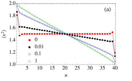
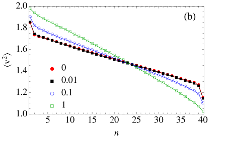
Figure 1: Average squared velocity $\langle v_{n}^{2}\rangle$ of the particles as a function of the position $n$ on the chain, which is in contact with heat reservoirs at temperatures $T_{A}=2$ and $T_{B}=1$. Results are given for a chain of $L=40$ particles for the values of $\lambda$ indicated, for the (a) harmonic case and (b) anharmonic case. In (a) the continuous lines are exact results.

The first and last particles are connected to heat baths at temperatures $T_{A}$ and $T_{B}$, and all particles are susceptive to stochastic collisions, here described by forces ${\cal F}_{n}(t)$. Denoting by $v_{n}=dx_{n}/dt$ the velocity of the $n$-th particle, the equations of motion are stochastic equations given by

$$m\frac{dv_{1}}{dt}=F_{1}+{\cal F}_{1}(t)-\alpha v_{1}+\sqrt{2\alpha k_{B}T_{A}}\xi_{A},$$ (5)

$$m\frac{dv_{n}}{dt}=F_{n}+{\cal F}_{n}(t),\qquad 2\leq n\leq L-1,$$ (6)

$$m\frac{dv_{L}}{dt}=F_{L}+{\cal F}_{L}(t)-\alpha v_{L}+\sqrt{2\alpha k_{B}T_{B}}\xi_{B},$$ (7)

where $k_{B}$ is Boltzmann constant and the last two terms in equations (5) and (7) represent the coupling to the heat reservoirs. The constant $\alpha$ represents the strength of the coupling and $\xi_{A}$ and $\xi_{B}$ are independent Gaussian white noises with zero mean and unit variance. The forces ${\cal F}_{n}(t)$ have the form of impulsive shot noises, given by

$${\cal F}_{n}=-2m\sum_{\ell=1}^{\infty}v_{n}(t_{n\ell}^{-})\delta(t-t_{n\ell}),$$ (8)

where $t_{n\ell},\ell=1,2,\ldots$ are uncorrelated exponentially distributed stochastic waiting times with a probability density distribution $\rho(t)=\lambda e^{-\lambda t}$. Here, the parameter $\lambda$ is the rate of collisions, which has been taken to be the same for all particles. After a collision occurring at time $t$, the $n$-th particle changes its velocity from $v_{n}(t^{-})$ to $v_{n}(t^{+})=-v_{n}(t^{-})$, thus conserving its kinetic energy and therefore the total energy

$$E=\sum_{n=1}^{L}\frac{m}{2}v_{n}^{2}+V(x).$$ (9)

Due to the contact with the reservoirs, the total energy $E$ is not a strictly conserved quantity. From the stochastic equations of motion we find

$$\frac{dE}{dt}={\cal J}_{A}+{\cal J}_{B},$$ (10)

where

$${\cal J}_{A}=-\alpha v_{1}^{2}+v_{1}\sqrt{2\alpha k_{B}T_{A}}\xi_{A},$$ (11)

and

$${\cal J}_{B}=-\alpha v_{L}^{2}+v_{L}\sqrt{2\alpha k_{B}T_{B}}\xi_{B}.$$ (12)

In the stationary state, $\langle E\rangle$ is a constant and the sum of the fluxes $J_{A}=\langle{\cal J}_{A}\rangle$ and $J_{B}=\langle{\cal J}_{B}\rangle$ vanishes, that is, $J_{B}=-J_{A}$. The heat flux $J=J_{A}$ can be calculated as the average of the right-hand side of equation (11) or in a equivalent way from the equation

$$J=K_{1}\langle(x_{n-1}-x_{n})v_{n}\rangle+K_{2}\langle(x_{n-1}-x_{n})^{3}v_{n}\rangle,$$ (13)

which we found to be numerically more accurate than the formula $J=\langle{\cal J}_{A}\rangle$.

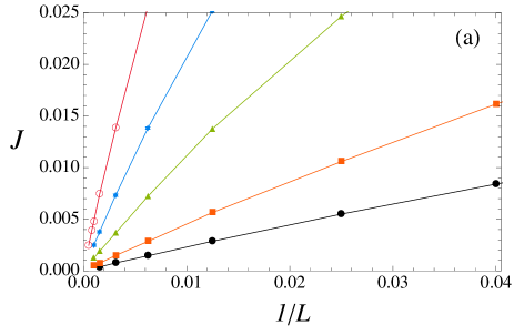
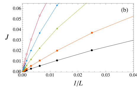
Figure 2: Heat flux $J$ as a function of the inverse of the system size $L$ for several values of $\lambda$ for (a) the harmonic chain and (b) the anharmonic chain. In both cases, from top to bottom, $\lambda=0.05,0.1,0.2,0.5$ and $1$. The temperatures of the reservoirs are $T_{A}=2$ and $T_{B}=1$. In (a) the continuous lines are exact results.

III Numerical solutions

The stochastic equations of motion were solved numerically for chains of several sizes $L$. This was done by discretizing the time in intervals $\Delta t$. We use an approach in which the deterministic part of the equations of motion of the inner particles are handled by the use of the Verlet algorithm verlet67 so as to ensure that, in the absence of the heat baths, energy is conserved. For the equations of motion of the first and last particles, which contain the stochastic forces due to the heat baths, we used the stochastic Verlet algorithm developed in paterlini98 . As for the stochastic shot noises we treat them as follows. At each time step, the sign of the velocity of each particle is changed with probability $p=\lambda\Delta t$. This procedure generates a Poisson process with discrete waiting time $t=\ell\Delta t$ that is distributed according to the probability distribution $p(1-p)^{\ell}$. In the continuous time limit, $\Delta t\to 0$, this yields the exponential distribution $\lambda e^{-\lambda t}$, as required.

For definiteness, our numerical calculations were performed with $k_{B}=1$, $m=1$, $\alpha=1$ and $\Delta t=0.01$. For the anharmonic potential all results reported in this paper were obtained for $K_{1}=1$ and $K_{2}=1$. The size of the system ranged from $L=10$ up to $L=5000$. We also present numerical results for the harmonic case ($K_{2}=0$), for $K_{1}=1$ and compare with the results of the anharmonic case. The existing exact solution dhar11 for harmonic case is used to check our numerical procedure. The exact solution is obtained by solving the equations for the pair correlations, which is possible because they consist of closed equations. However, this closure property does not happen for the anharmonic case.

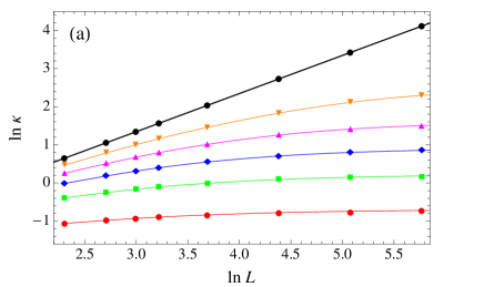
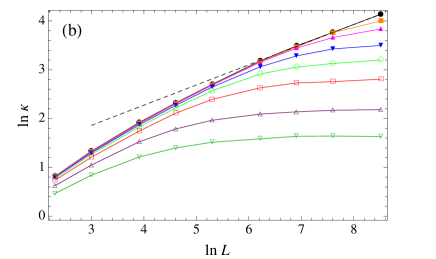
Figure 3: Log-log plot of the heat conductivity $\kappa$ as a function of the system size $L$ for (a) the harmonic chain and (b) the anharmonic chain. From top to bottom, $\lambda=0,0.02,0.05,0.1,0.2$ and $0.5$, for (a) and $\lambda=0,0.001,0.002,0.005,0.01,0.02,0.05$ and $0.1$, for (b). The temperatures of the reservoirs are $T_{A}=2$ and $T_{B}=1$. In (a), the continuous lines are exact results and the slope of the straight line corresponding to $\lambda=0$ is $a=1$. In (b), the slope of the straight line (dashed line) fitted to the data points with large $L$ corresponding to $\lambda=0$ gives $a=0.42$.

In Fig. 1 we show the results for the average kinetic energy for each particle as a function of the position $n$ on the chain for the harmonic and anharmonic cases. The temperatures of the reservoirs are considered to be distinct, $T_{A}\neq T_{B}$, and our numerical calculations were performed for $T_{A}=2$ and $T_{B}=1$. Without stochastic collisions ($\lambda=0$) the results of the harmonic case shows that the kinetic energy is almost constant, a result obtained by Rieder et al rieder67 , which does not lead to Fourier’s Law. The inclusion of the stochastic collisions ($\lambda\neq 0$) produces a drastically different result. The average kinetic energy as a function of $n$ displays now a nonzero slope as can be seen in Fig. 1. For the anharmonic case, all curves, including the case $\lambda=0$, show a nonzero slope. In spite of that, the $\lambda=0$ case does not lead to Fourier’s law.

We have calculated the flux $J$ at the stationary state by using equation (13) and the results are shown in Fig. 2 as a function of $1/L$ for several values of $\lambda$. From this figure we see clearly that $J\sim 1/L$, for sufficiently large values of $L$, in accordance with Fourier’s law, as long as $\lambda\neq 0$, for both harmonic and anharmonic cases. For sufficiently large values of $L$ the heat conductivity is given by $\kappa=JL/\Delta T$. This quantity is plotted as a function of $L$ for several values of the rate of stochastic collisions $\lambda$, including $\lambda=0$. The results are shown in Fig. 3. For both the harmonic and anharmonic cases, the heat conductivity $\kappa$ approaches a constant when $L\to\infty$, as long as $\lambda\neq 0$, and Fourier’s law is accomplished. When $\lambda=0$, our numerical results gives a superdiffusive behavior with $\kappa\to\infty$ when $L\to\infty$, according to

$$\kappa\sim L^{a},\qquad\qquad\lambda=0,$$ (14)

as shown in Fig. 3. For the harmonic case, $a=1$, which is in accordance with the result by Rieder et al rieder67 . For the anharmonic case we get $a=0.42\pm 0.04$. This is in agreement with the result $a=0.45\pm 5$ found by Lepri et al. lepri97 and in excelent agreement with the value $a=2/5$ lepri03 ; lukkarinen08 .

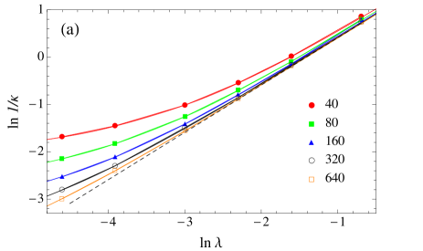
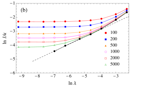
Figure 4: Log-log plot of the reciprocal of the heat conductivity $\kappa$ as a function of the collision noise $\lambda$ for (a) the harmonic chain and (b) the anharmonic chain, for several values of $L$ indicated. The temperatures of the reservoirs are $T_{A}=2$ and $T_{B}=1$. In (a) the continuous lines are exact results. The slope of the straight dashed lines is $b=1$ for (a) the harmonic case and $b=0.52$ for the (b) anharmonic case. The lowest curve in both cases are extrapolation obtained from finite values of $L$.

To analyze the behavior of the heat conductivity $\kappa=JL/\Delta T$ as $\lambda\to 0$ we have plotted this quantity as a function of $\lambda$ for several values of the system size $L$. The results are shown in Fig. 4. We have plotted also the extrapolated values of $\kappa$ when $L\to\infty$ for each $\lambda$. These extrapolated values were extracted from the plot of $1/\kappa$ versus $1/L$. The heat conductivity $\kappa$ diverges when $\lambda\to 0$ according to

$$\kappa\sim\lambda^{-b},\qquad\qquad L\to\infty.$$ (15)

For the harmonic case our results give $b=1$, a result obtained by Dhar et al dhar11 . For the anharmonic case we found $b=0.52\pm 0.06$, a result clearly distinct from the harmonic case.

The algebraic behavior of $\kappa$ with $L$ and $\lambda$ can be obtained by assuming the following finite-size scaling for the heat conductivity,

$$\kappa=L^{a}\psi(\lambda L^{c}),$$ (16)

where $\psi(s)$ is a universal function of $s=\lambda L^{c}$ such that $\psi(0)$ is a finite constant and $\psi(s)\sim s^{-b}$ when $s$ is large. To ensure a finite conductivity in the limt $L\to\infty$, the exponent $c$ must be related to the exponents $a$ and $b$ by $c=a/b$. In Fig. 5, we show the data collapse for the harmonic case by plotting $\kappa/L^{a}$ as a function of $\lambda L^{c}$, where in this case $a=1$ and $c=1$. The data collapse is well described by the expression

$$\psi(s)=\frac{A}{B+s},$$ (17)

as can be seen in Fig. 5. This function was obtained by numerically solving the exact equations for the pair correlations from which we found $A=1/4$ and $B=3/2$. For large values of $s$, this result gives $\psi\sim s^{-1}$ so that $\kappa\sim\lambda^{-1}$, independent of $L$, which is the behavior of the conductivity for the harmonic chain when $L\to\infty$ bolsterli70 ; bonetto04 ; dhar11 . For the anharmonic case, the data colapse, shown in Fig. 5, was obtained by using the exponents $a$ and $b$ obtained previously.

It is worth mentioning that Lepri et al. lepri09 in their study of a one-dimensional harmonic crystal with energy conservative noise consisting of elastic collisions between neighboring particles reported a conductivity that behaves as $(L/\lambda)^{1/2}$ for large values of $L$. Assuming for this system a scaling function of the form (16) and keeping in mind that $a=1$, because the conductivity behaves as $\kappa\sim L$ when $\lambda=0$, we may conclude that $b=1/2$ and $c=1$. Notice, however, that $c\neq a/b$ so that $\kappa$ is not finite but diverges when $L\to\infty$.

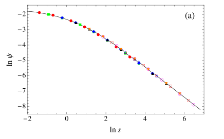
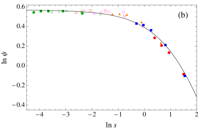
Figure 5: Data colapse obtained from the numerical results of the heat conductivity $\kappa$ obtained from several values of $\lambda$ and $L$ corresponding to the harmonic case (a) and the anharmonic case (b), where $\Psi=\kappa/L^{a}$ and $s=\lambda L^{a/b}$. The continuous line in case (a) is described by the expression (17) with $A=1/4$ and $B=3/2$. In case (b), the continous line is a guide to the eyes. The temperatures of the reservoirs are $T_{A}=2$ and $T_{B}=1$. Points with the same symbol correspond to the same value of $\lambda$.

A relevant feature of the present anharmonic chain with random reversal of velocities is the dependence of the heat conductivity with temperature. For the harmonic case the heat conductivity is temperature independent bolsterli70 ; dhar11 , a result that can be understood by using the following reasoning. If we rescale the temperature of the reservoirs by a factor $r$, that is, $T_{A}\to rT_{A}$ and $T_{B}\to rT_{B}$, and the positions and velocities by a factor $r^{1/2}$, that is, $v_{n}\to r^{1/2}v_{n}$ and $x_{n}\to r^{1/2}x_{n}$, the equations of motions for the case $K_{2}=0$ become invariant. In addition, according to Eq. (13) with $K_{2}=0$, the heat flux changes as the temperature, that is, $J\to rJ$. From this relation it follows that $J$ is a homogeneous function of $T_{A}$ and $T_{B}$, so that $J=T_{A}\phi(T_{B}/T_{A})$. Writing $T_{B}=T_{A}+\Delta T$, then for small values of $\Delta T$ it follows that $J\sim\Delta T$ leading to a heat conductivity $\kappa$ independent of temperature, a result that we have also checked numerically.

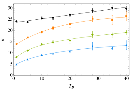
Figure 6: Heat conductivity $\kappa=JL/\Delta T$ as a function of the temperature $T=T_{B}$ of the colder reservoir, for several values of $\lambda$. From top to bottom $\lambda=0,0.02,0.05$ and $0.1$. All results were obtained for a chain of size $L=500$ and by using the same value of the difference in temperature of the reservoirs, $\Delta T=1$. The continuous lines are guide to the eyes.

For the anharmonic case we have found that the heat conductivity $\kappa$ is an increasing function of temperature. In Fig. 6 we show $\kappa$ as a function of the temperature $T=T_{B}$ of the colder reservoir, The heat conductivity was determined from $\kappa=JL/\Delta T$, for the same value of $\Delta T=1$ and for several values of the noise parameter $\lambda$. We used $L=500$, a value high enough so that the values of $\kappa$ may be considered the asympototic values (see Fig. 3), with the exception of the case $\lambda=0$. Our results indicate a monotonic increase of the heat conductivity with temperature as can be seen in Fig. 6. We have found that our results are consistent with the result of Aoki and Kusnezov aoki01 and with the upper bounds of Bernardin and Olla bernardin11 .

IV Conclusion

In conclusion, we have considered a chain of particles interacting through anharmonic potentials and subject to heat reservoirs at its ends. In addition, the chain is subject to a shot noise that changes the sign of the velocities of the particles at random times, distributed according to an exponential distribution. The shot noise does not change the energy so that the changes in energy are only due to the contact with the reservoirs. We have shown that, when the chain is connected to reservoirs at different temperatures, the heat flux is inversely proportional to the size of the system, as long as the shot noise parameter $\lambda$ is nonzero, and therefore in accordance with Fourier’s law. Our results suggest, in accordance with bolsterli70 , that the ergodicity may play a crucial role in the derivation of Fourier’s law.

We have also obtained the behavior of $\kappa$ with $L$ when $\lambda=0$ and $\kappa$ with $\lambda$ when $L\to\infty$. Both behaviors are found to be algebraic, characterized by exponents $a=0.42\pm 0.04$ and $b=0.52\pm 0.06$. This allows us to introduce a finite-size scaling in which the noise parameter scales with the inverse of the system size to the power $a=b/c$. For the harmonic case, we have shown that a finite size scaling exists, a result that has been also obtained by numerically solving the equations for the correlations.

References

- (1) Z. Rieder, J. L. Lebowitz and E. Lieb, J. Math. Phys. 8, 1073 (1967).
- (2) S.Lepri, R. Livi and A. Politi, Phys. Rev. Lett. 78, 1896 (1997).
- (3) A. Dhar, Phys. Rev. Lett. 86, 3554 (2001).
- (4) O. Narayan and S. Ramaswamy, Phys. Rev. Lett. 89, 200601 (2002).
- (5) P. Grassberger, W. Nadler and L. Yang, Phys. Rev. Lett. 89, 180601 (2002).
- (6) G. Casati and T. Prozen, Phys. Rev. E 67, 015203R (2003).
- (7) J. M. Deutsch and O. Narayan, Phys. Rev. E 68, 010201R (2003).
- (8) S. Lepri, R. Livi and A. Politi, Phys. Rep. 377, 1 (2003).
- (9) J.-P. Eckmann and L.-S. Young, Europhys. Lett. 68, 790 (2004).
- (10) E. Pereira and R. Falcão, Phys. Rev. E 70, 046105 (2004).
- (11) F. Bonetto, J. L. Lebowitz and J. Lukkarinen, J. Stat. Phys. 116, 783 (2004).
- (12) P. Cipriani, S. Denisov and A. Politi, Phys. Rev. Lett. 94, 244301 (2005).
- (13) E. Pereira and R. Falcão, Phys. Rev. Lett. 96, 100601 (2006).
- (14) L. Delfini, S. Lepri, R. Livi and A. Politi, Phys. Rev. E 73, 060201 (2006).
- (15) T. Mai, A. Dhar and O. Narayan, Phys. Rev. Lett. 98, 184301 (2007).
- (16) E. Pereira and H. C. F. Lemos, Phys. Rev. E 78, 031108 (2008).
- (17) J. Lukkarinen and H. Spohn, Commun. Pure Appl.Math. 61, 1753 (2008).
- (18) A. Dhar, Adv. Phys. 57, 457 (2008).
- (19) G. Basile, C. Bernardin and S. Olla, Commun. Math. Phys. 287, 67 (2009).
- (20) A. Iacobucci, F. Legoll, S. Olla and G. Stolz, J. Stat. Phys. 140, 336 (2010).
- (21) A. Gerschenfeld, B. Derrida and J. L. Lebowitz, J. Stat. Phys. 141, 757 (2010).
- (22) A. Dhar, K. Venkateshan and J. L. Lebowitz, Phys. Rev. E 83, 021108 (2011).
- (23) H. van Beijeren, Phys. Rev. Lett. 108, 180601 (2012).
- (24) N. W. Ashcroft and N. D. Mermin, Solid State Physics (Holt, Rinehart and Winston, New York, 1976).
- (25) R. E. Peierls, Quantum Theory of Solids (Clarendon Press, Oxford, 1955).
- (26) Y. Dubi and M. Di Ventra, Phys. Rev. E 79, 042101 (2009).
- (27) Y. Dubi and M. Di Ventra, Phys. Rev. B 79, 115415 (2009).
- (28) M. Bolsterli, M. Rich and W. M. Visscher, Phys. Rev. A 1, 1086 (1970).
- (29) D. Roy, Phys. Rev. E 86, 041102 (2012).
- (30) L. Verlet, Phys. Rev. 159, 98 (1967).
- (31) M. G. Paterlini and D. M. Ferguson, Chem. Phys. 236, 243 (1998).
- (32) S. Lepri, C. Mejía-Monasterio and A. Politi, J. Phys. A: Math. Theor. 42, 025001 (2009).
- (33) K. Aoki and D. Kusnezov, Phys. Rev. Lett. 86, 4029 (2001).
- (34) C. Bernardin and S. Olla, J. Stat. Phys. 145, 1244 (2011).