Cell body rocking is a dominant mechanism for flagellar synchronization in a swimming alga

Abstract

The unicellular green algae Chlamydomonas swims with two flagella, which can synchronize their beat. Synchronized beating is required to swim both fast and straight. A long-standing hypothesis proposes that synchronization of flagella results from hydrodynamic coupling, but the details are not understood. Here, we present realistic hydrodynamic computations and high-speed tracking experiments of swimming cells that show how a perturbation from the synchronized state causes rotational motion of the cell body. This rotation feeds back on the flagellar dynamics via hydrodynamic friction forces and rapidly restores the synchronized state in our theory. We calculate that this ‘cell body rocking’ provides the dominant contribution to synchronization in swimming cells, whereas direct hydrodynamic interactions between the flagella contribute negligibly. We experimentally confirmed the coupling between flagellar beating and cell body rocking predicted by our theory. We propose that the interplay of flagellar beating and hydrodynamic forces governs swimming and synchronization in Chlamydomonas.

This work appeared also in the Proceedings of the National Academy of Science of the U.S.A as:

Geyer et al., Proc. Natl. Acad. Sci. U.S.A., 110(45), p. 18058(6), 2013.

Eukaryotic cilia and flagella are long, slender cell appendages that can bend rhythmically and thus represent a prime example of a biological oscillator Alberts:cell . The flagellar beat is driven by the collective action of dynein molecular motors, which are distributed along the length of the flagellum. The beat of flagella, with typical frequencies ranging from $20-60\,\mathrm{Hz}$, pumps fluids, e.g. mucus in mammalian airways Sanderson:1981 , and propels unicellular micro-swimmers like Paramecium, spermatozoa, or algae Gray:1928 . The coordinated beating of collections of flagella is important for efficient fluid transport Sanderson:1981 ; Osterman:2011 and fast swimming Brennen:1977 . This coordinated beating represents a striking example for the synchronization of oscillators, prompting the question of how flagella couple their beat. Identifying the specific mechanism of synchronization can be difficult as synchronization may occur even for weak coupling Pikovsky:synchronization . Further, the effect of the coupling is difficult to detect once the synchronized state has been reached.

Hydrodynamic forces were suggested to play a significant role for flagellar synchronization already in 1951 by G.I. Taylor Taylor:1951 . Since then, direct hydrodynamic interactions between flagella were studied theoretically as a possible mechanism for flagellar synchronization Gueron:1999 ; Vilfan:2006 ; Niedermayer:2008 ; Golestanian:2011 . Another synchronization mechanism that is independent of hydrodynamic interactions was recently described in the context of a minimal model swimmer Friedrich:2012c ; Bennett:2013 ; Polotzek:2013 . This mechanism crucially relies on the interplay of swimming motion and flagellar beating.

Here, we address the hydrodynamic coupling between the two flagella in a model organism for flagellar coordination Ruffer:1985a ; Ruffer:1998a ; Polin:2009 ; Goldstein:2009 , the unicellular green algae Chlamydomonas. Chlamydomonas propels its ellipsoidal cell body, which has typical diameter $10\,{\mu\mathrm{m}}$, using a pair of flagella, whose lengths are about $10\,{\mu\mathrm{m}}$ Ruffer:1985a . The two flagella beat approximately in a common plane, which is collinear with the long axis of the cell body. In that plane, the two beat patterns are nearly mirror-symmetric with respect to this long axis. The beating of the two flagella of Chlamydomonas can synchronize, i.e. adopt a common beat frequency and a fixed phase relationship Ruffer:1985a ; Ruffer:1998a ; Polin:2009 ; Goldstein:2009 . In-phase synchronization of the two flagella is required for swimming along a straight path Goldstein:2009 . The specific mechanism leading to flagellar synchrony is unclear.

Here, we use a combination of realistic hydrodynamic computations and high-speed tracking experiments to reveal the nature of the hydrodynamic coupling between the two flagella of free swimming Chlamydomonas cells. Previous hydrodynamic computations for Chlamydomonas used either resistive force theory Tam:2011 ; Bayly:2011 , which does not account for hydrodynamic interactions between the two flagella, or computationally intensive finite element methods Malley:2012 . We employ an alternative approach and represent the geometry of a Chlamydomonas cell by spherical shape primitives, which provides a computationally convenient method that fully accounts for hydrodynamic interactions between different parts of the cell. Our theory characterizes flagellar swimming and synchronization by a minimal set of effective degrees of freedom. The corresponding equation of motion follows naturally from the framework of Lagrangian mechanics, which was used previously to describe synchronization in a minimal model swimmer Friedrich:2012c . These equations of motion embody the basic assumption that the flagellar beat speeds up or slows down according to the hydrodynamic friction forces acting on the flagellum. This assumption is supported by previous experiments, which showed that the flagellar beat frequency depends on the viscosity of the surrounding fluid if the concentration of the chemical fuel ATP is sufficiently high Brokaw:1975 . The simple force-velocity relationship for the flagellar beat employed by us coarse-grains the behavior of thousands of dynein molecular motors that collectively drive the beat. Similar force-velocity properties have been described for individual molecular motors Hunt:1994 and reflect a typical behavior of active force generating systems.

Our theory predicts that any perturbation of synchronized beating results in a significant yawing motion of the cell, reminiscent of rocking of the cell body. This rotational motion imparts different hydrodynamic forces on the two flagella, causing one of them to beat faster and the other to slow down. This interplay between flagellar beating and cell body rocking rapidly restores flagellar synchrony after a perturbation. Using the framework provided by our theory, we analyze high-speed tracking experiments of swimming cells, confirming the proposed two-way coupling between flagellar beating and cell body rocking.

Previous experiments restrained Chlamydomonas cells from swimming, holding their cell body in a micropipette Ruffer:1998a ; Polin:2009 ; Goldstein:2009 . Remarkably, flagellar synchronization was observed also for these constrained cells. This observation seems to argue against a synchronization mechanism that relies on swimming motion. However, the rate of synchronization observed in these experiments was faster by an order of magnitude than the rate we predict for synchronization by direct hydrodynamic interactions between the two flagella in the absence of any motion. In contrast, we show that rotational motion with a small amplitude of a few degrees only, which may result from either a residual rotational compliance of the clamped cell or an elastic anchorage of the flagellar pair, provides a possible mechanism for rapid synchronization, which is analogous to synchronization by cell body rocking in free-swimming cells.

I Results and Discussion

I.1 High-precision tracking of confined Chlamydomonas cells

To study the interplay of flagellar beating and swimming motion, we recorded single wild-type Chlamydomonas reinhardtii cells swimming in a shallow observation chamber using high-speed phase-contrast microscopy (1000 fps). The chamber heights were only slightly larger than the cell diameter so that the cells did not roll around their long body axis, but only translated and rotated in the focal plane. This confinement of cell motion to two space dimensions and the fact that the approximately planar flagellar beat was parallel to the plane of observation greatly facilitated data acquisition and analysis. From high-speed recordings, we obtained the projected position and orientation of the cell body as well as the shape of the two flagella, see figure 1A.

In a reference frame of the cell body, each flagellum undergoes periodic shape changes. To formalize this observation, we defined a flagellar phase variable by binning flagellar shapes according to shape similarity, see figure 1B. A time-series of flagellar shapes is represented by a point cloud in an abstract shape space. This point cloud comprises an effectively one-dimensional shape cycle, which reflects the periodicity of the flagellar beat. Each shape point can be projected on the centerline of the point cloud. We define a phase variable $\varphi$ running from $0$ to $2\pi$ that parametrizes this limit cycle by requiring that the phase speed $\dot{\varphi}$ is constant for synchronized beating. Approximately, we determine this parametrization from the condition that the averaged phase speed is independent of the location along the limit cycle. This defines a unique flagellar phase for each tracked flagellar shape. The width of the point cloud shown in figure 1B is a measure for the variability of the flagellar beat during subsequent beat cycles. We find that the variations of flagellar shapes for the same value of the phase variable are much smaller than the shape changes during one beat cycle. For our analysis, we therefore neglect these variations of the flagellar beat. In this way, we characterize a swimming Chlamydomonas cell by $5$ degrees of freedom: its position $(x,y)$ in the plane, the orientation angle $\alpha$ of its cell body, and the two flagellar phase variables $\varphi_{L}$ and $\varphi_{R}$ for the left and right flagellum, respectively. Our theoretical description will employ the same $5$ degrees of freedom and use flagellar shapes tracked from experiment for the hydrodynamic computations.

I.2 Hydrodynamic forces and interactions

For a swimming Chlamydomonas cell, inertial forces are negligible (as characterized by a low Reynolds number of $\mathrm{Re}\sim 10^{-3}$ Malley:2012 ), which implies that the hydrodynamic friction forces exerted by the cell depend only on its instantaneous motion Happel:hydro . To conveniently compute hydrodynamic friction forces and hydrodynamic interactions, we represented the geometry of a Chlamydomonas cell by $N=300$ spherical shape primitives, see figure 2A. The spheres constituting the cell body are treated as a rigid cluster. For simplicity, we consider free swimming cells and do not include wall effects in our hydrodynamic computations. Flagellar beating and swimming corresponds to a simultaneous motion of all $300$ spheres of our cell model. The dependence of the corresponding hydrodynamic friction forces and torques on the velocities of the individual spheres is characterized by a grand hydrodynamic friction matrix $\mathrm{G}$. We computed this friction matrix $\mathrm{G}$ using a Cartesian multipole expansion technique Hinsen:1995 , see ‘Materials and Methods’ for details. Figure 2C,D shows a sub-matrix that relates force and velocity components parallel to the long axis of the cell. The entries of the color matrix depict the force exerted by any of the flagellar spheres or by the cell body cluster (row index), if a single flagellar sphere or the cell body cluster is moved (column index). The indexing of flagellar spheres is indicated by cartoon drawings of the cell next to the color matrix. The diagonal entries of this friction matrix are positive and account for the usual Stokes friction of a single ‘flagellar sphere’ (or of the cell body). Off-diagonal entries are negative and represent hydrodynamic interactions. We find considerable hydrodynamic interactions between spheres of the same flagellum, as well as between each flagellum and the cell body. However, interactions between the two flagella are comparably weak.

I.3 Theoretical description of flagellar beating and swimming

We present dynamical equations for the minimal set of 5 degrees of freedom shown in figure 1A to describe flagellar beating, swimming, and later flagellar synchronization in Chlamydomonas. These equations of motion follow naturally from the framework of Lagrangian mechanics of dissipative systems, which defines generalized forces conjugate to effective degrees of freedom.

Motivated by our experiments, we describe the progression through subsequent beat cycles of each of the two flagella by respective phase angles $\varphi_{L}$ and $\varphi_{R}$, see figure 1A. The angular frequency $\omega_{j}$ of flagellar beating is given by the time-averaged phase speed $\langle\dot{\varphi}_{j}\rangle$, so we can think of the phase speed as the instantaneous beat frequency. We are interested in variations of the phase speed that can restore a synchronized state after a perturbation. We introduce the key assumption that changes in hydrodynamic friction during the flagellar beat cycle can increase or decrease the phase speed of each flagellum. Specifically, we assume that for both the left and right flagellum, $j=L,R$, the respective flagellar phase speed $\dot{\varphi}_{j}$ is determined by a balance of an active driving force $Q_{j}$ that coarse-grains the active processes within the flagellum and a generalized hydrodynamic friction force $P_{j}$, which depends on $\dot{\varphi}_{j}$. Note that in addition to hydrodynamic friction, dissipative processes within the flagella may contribute to the friction forces $P_{L}$ and $P_{R}$. We do not consider such internal friction in our description as it does not change our results qualitatively. The hydrodynamic friction forces $P_{j}$ have to be computed self-consistently for a swimming cell. We restrict our analysis to planar motion in the ‘$xy$’-plane and thus consider the position $(x,y)$ and the orientation $\alpha$ of the cell body with respect to a fixed laboratory frame, see figure 1A.

Any change of the degrees of freedom $x$, $y$, $\alpha$, $\varphi_{L}$, $\varphi_{R}$ results in the dissipation of energy into the fluid at some rate $\mathcal{R}$. This dissipation rate $\mathcal{R}$ characterizes the mechanical power output of the cell and plays the role of a Rayleigh dissipation function known in Lagrangian mechanics; it can be written as $\mathcal{R}=\dot{x}P_{x}+\dot{y}P_{y}+\dot{\alpha}P_{\alpha}+\dot{\varphi}_{L}P_{L}+\dot{\varphi}_{R}P_{R}$, which defines the generalized friction forces conjugate to the different degrees of freedom. The forces $P_{L}$, $P_{R}$, $P_{\alpha}$ are conjugate to an angle and have physical unit $\mathrm{pN}\,\mu\mathrm{m}$. We compute the generalized friction forces using the grand hydrodynamic friction matrix $\mathrm{G}$ introduced above. In brief, the superposition principle of low Reynolds number hydrodynamics relevant for Chlamydomonas swimming Happel:hydro implies that the generalized friction forces relate linearly to the generalized velocities, $P_{j}=\Gamma_{jx}\dot{x}+\Gamma_{jy}\dot{y}+\Gamma_{j\alpha}\dot{\alpha}+\Gamma_{jL}\dot{\varphi}_{L}+\Gamma_{jR}\dot{\varphi}_{R}$. This defines the generalized hydrodynamic friction coefficients $\Gamma_{ji}$, which are suitable linear combinations of the entries of the grand hydrodynamic friction matrix $\mathrm{G}$, see ‘Materials and Methods’.

The friction force $P_{x}$ conjugate to the $x$-coordinate of the cell position represents just the $x$-component of the total force exerted by the cell on the fluid, an analogous statement applies for $P_{y}$; $P_{\alpha}$ is the total torque associated with rotations around an axis normal to the plane of swimming. If the swimmer is free from external forces and torques, we have $P_{x}=P_{y}=0$ and $P_{\alpha}=0$. Together with the proposed balance of flagellar friction and driving forces, $P_{L}=Q_{L}$ and $P_{R}=Q_{R}$, we have a total of 5 force balance equations, which allow us to solve for the time derivatives of the 5 degrees of freedom. We obtain an equation of motion that combines swimming and flagellar phase dynamics

$$(\dot{x},\dot{y},\dot{\alpha},\dot{\varphi}_{L},\dot{\varphi}_{R})^{T}=\Gamma^{-1}(0,0,0,Q_{L},Q_{R})^{T}.$$ (1)

The phase dependence of the active driving forces $Q_{j}(\varphi_{j})$ is uniquely specified by the condition that the phase speeds should be constant, $\dot{\varphi}_{j}=\omega_{0}$, for synchronized flagellar beating with zero flagellar phase difference $\delta=0$, where $\delta=\varphi_{L}-\varphi_{R}$.

In essence, this generic description implies that the phase speed of one flagellum is determined by hydrodynamic friction forces, which in turn depend on the swimming motion of the cell. Since the swimming motion is determined by the beating of both flagella, equation 1 effectively defines a feedback loop that couples the two flagellar oscillators.

I.4 Theory and experiment of Chlamydomonas swimming

Using the equation of motion (equation 1), we can compute the swimming motion of our model cell. For mirror-symmetric flagellar beating with zero flagellar phase difference $\delta=0$, the model cell follows a straight path with an instantaneous velocity that is positive during the effective stroke, but becomes negative during a short period of the recovery stroke (figure 3A, left panel). The cell swims two steps forward, one step back. This saltatory motion is also observed experimentally by us (figure 3A, middle panel) and others Racey:1981 ; Ruffer:1985a ; Guasto:2010 . In our computation, the instantaneous swimming velocity reaches values up to $200\,\mu\mathrm{m}/\mathrm{s}$, which agrees with experimental measurements for free-swimming cells Guasto:2010 , but overestimates the observed translational swimming speeds in shallow chambers, in which wall effects are expected to reduce the speed of translational motion (compare left and right panels in figure 3A). If the two flagella are beating out of phase, the cell will not swim straight anymore, but the cell body yaws, see figure 3B. Cell body yawing is observed experimentally (right panel), with measured yawing rates that agree well with our computations (left panel). The proximity of boundary walls is known to reduce translational motion, but to affect rotational motion to a much lesser extent for a given distance from the wall Bayly:2011 . This is indeed observed in our experiments with cells swimming in shallow chambers: while the observed translational speed is smaller than predicted (figure 3A), the observed yawing rates are very similar to the predicted ones (figure 3B). The good agreement between theory and experiment for the yawing rate supports our hydrodynamic computation as well as our description of flagellar beating using a single phase variable. In the next section, we show that rotational motion is crucial for flagellar synchronization, while translational motion is less important.

I.5 Theory of flagellar synchronization by cell body yawing

We now demonstrate how yawing of the cell body leads to flagellar synchronization. We first examine the flagellar phase dynamics after a perturbation of in-phase flagellar synchrony. Figure 4A shows numerical results for a free swimming cell obtained from solving the equation of motion (equation 1). The initial flagellar asynchrony causes a yawing motion of the model cell, which is characterized by periodic changes of the cell’s orientation angle $\alpha(t)$. The phase difference $\delta$ between the left and right flagellum decays approximately exponentially as $\delta(t)\sim\exp(-\lambda t/T)$ with a rate constant $\lambda$ [measured in beat periods $T=2\pi/\omega_{0}$] that will serve as a measure of the strength of synchronization.

To mimic experiments where external forces constrain cell motion, we now consider the idealized case of a cell that cannot translate, while cell body yawing is constrained by an elastic restoring force $Q_{\alpha}=-k\alpha$. Again, the two flagella synchronize in-phase, provided some residual cell body yawing is allowed, see figure 4B. In the absence of an elastic restoring force ($k=0$), when the model cell cannot translate, but can still freely rotate, its yawing motion and synchronization behavior is very similar to the case of a free swimming cell that can rotate and translate. For a fully clamped cell body, however, the synchronization strength is strongly attenuated, and is solely due to the direct hydrodynamic interactions between the two flagella. In this case of synchronization by hydrodynamic interactions, the time-constant for synchronization is decreased approximately 20-fold compared to the case of free swimming. These numerical observations point at a crucial role of cell body yawing for flagellar synchronization. The underlying mechanism of synchronization can be explained as follows. For in-phase synchronization, the flagellar beat is mirror-symmetric and the cell swims along a straight path. If, however, the left flagellum has a small head-start during the effective stroke, this causes a counter-clockwise rotation of the cell, see figure 3B. This cell body yawing increases (decreases) the hydrodynamic friction encountered by the left (right) flagellum, causing the left flagellum to beat slower and the right one to beat faster. As a result, flagellar synchrony is restored.

Next, we present a formalized version of this argument using a reduced equation of motion. We thus arrive at a simple theory for biflagellar synchronization, which will later allow for quantitative comparison with experiments. As in figure 4B, we assume that the cell is constrained such that it cannot translate ($\dot{x}=\dot{y}=0$). The cell can still yaw, possibly being subject to an elastic restoring force $Q_{\alpha}=-k\alpha$. This leaves only three degrees of freedom: $\varphi_{L}$, $\varphi_{R}$, and $\alpha$. Neglecting direct hydrodynamic interactions between the flagella, we can reduce the equations of motion for a clamped cell (equation 1 with constraint $\dot{x}=\dot{y}=0$) to a set of three coupled equations for the three remaining degrees of freedom

$$\dot{\varphi}_{L} =\omega_{L}-\mu(\varphi_{L})\dot{\alpha},$$ (2)

$$\dot{\varphi}_{R} =\omega_{R}+\mu(\varphi_{R})\dot{\alpha},$$ (3)

$$k\,\alpha+\rho(\varphi_{L},\varphi_{R})\,\dot{\alpha} =-\nu(\varphi_{L})\dot{\varphi}_{L}+\nu(\varphi_{R})\dot{\varphi}_{R}.$$ (4)

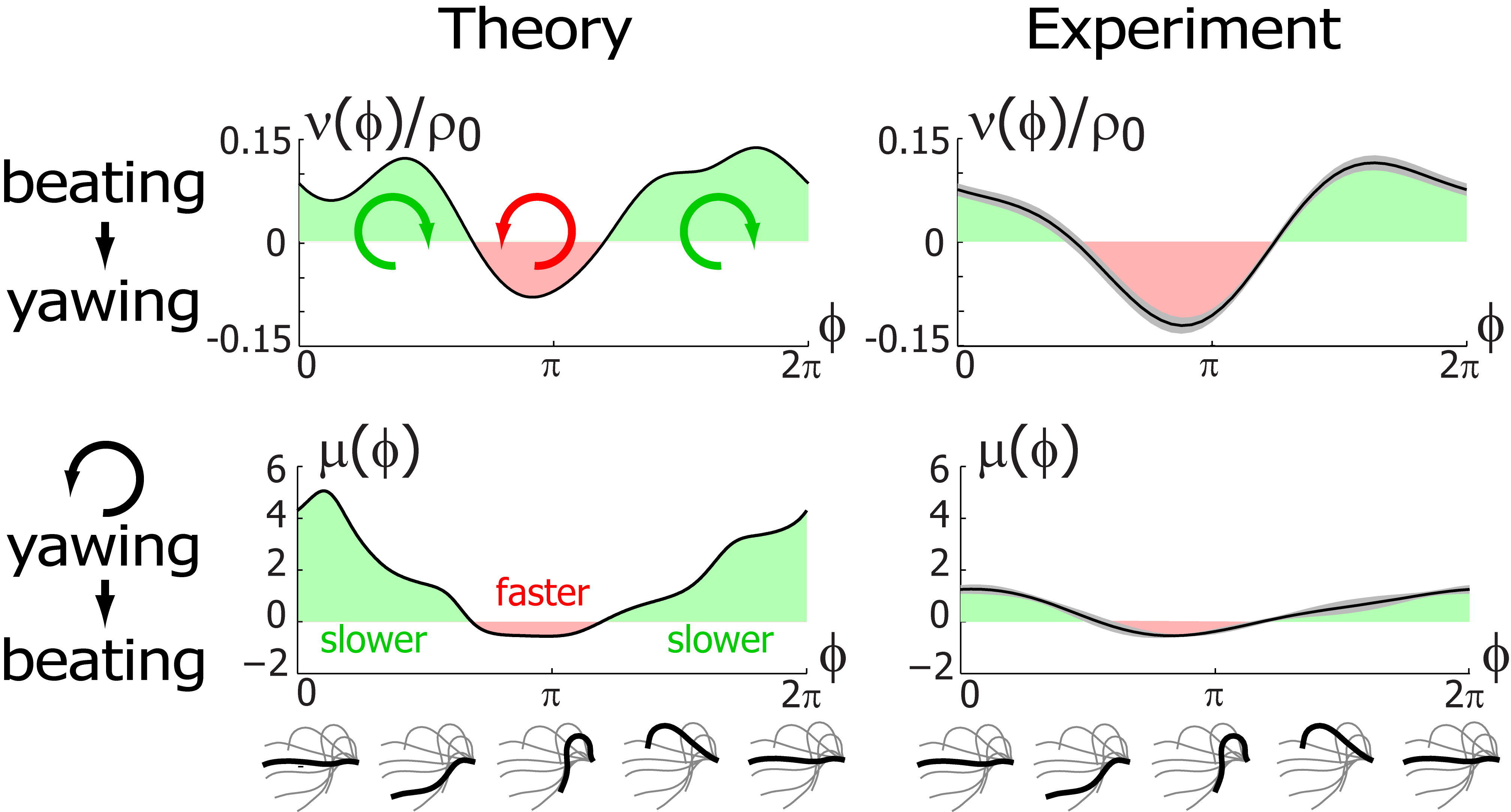
Figure 5: Flagellar beating and cell body yawing are coupled in a bidirectional way. Theory (left): In our theory, the beat of the left flagellum generates a torque, which, in the absence of the right flagellum, has to be counterbalanced by a yawing motion of cell body, see eqn. 4. This effect is quantified by the coupling function $\nu(\varphi)$ shown in the upper panel, normalized here by $\rho_{0}=\langle\rho\rangle$: the effective stroke ($\varphi_{L}\sim 0^{\circ}$) of the left flagellum causes the cell to yaw clockwise. Conversely, yawing of the cell changes the hydrodynamic friction force that opposes the flagellar beat, which, in our theory, speeds up or slows down the beat, see eqn. 2. This effect is quantified by the coupling function $\mu(\varphi)$ shown in the lower panel: a counter-clockwise yawing during the effective stroke of the left flagellum slows down its beat. The coupling of beating and yawing allows for flagellar synchronization in a free swimming cell. Experiment (right): By fitting eqns. 2 and 4 to experimental time series data, we can recover the coupling functions $\mu(\varphi)$ and $\nu(\varphi)/\rho_{0}$ (1 cell, $n=5$ time series of $0.5\,\mathrm{s}$ duration, gray regions denote mean$\pm$s.e.).

The coupling function $\mu$ in equation 2 characterizes the effect of cell body yawing on the flagellar beat as detailed below, while $\nu$ describes how asynchronous flagellar beating results in yawing; $\rho$ is the hydrodynamic friction coefficient for yawing of the whole cell. The coupling functions $\mu$, $\nu$, and $\rho$ can be computed using our hydrodynamic model. Their dependence on the flagellar phase is shown in figure 5 (left panels). The physical significance of equations 2-4 can be explained as follows: Equation 2 implies that during the effective stroke of the left flagellum ($\varphi\sim 0^{\circ}$), a counter-clockwise rotation of the whole cell slows down the flagellar beat, while a clockwise rotation speeds it up (figure 5B, $\mu>0$). Equation 3 implies the converse for the right flagellum. During the recovery stroke ($\varphi\sim 180^{\circ}$), the effect is opposite and a counter-clockwise rotation of the cell would speed up the beat of the left flagellum ($\mu<0$). Equation 4 states that flagellar beating causes the cell body to yaw: if the right flagellum were absent, the model cell rotates clockwise ($\dot{\alpha}<0$) during the effective stroke of the left flagellum (figure 5A, $\nu>0$), and counter-clockwise during its recovery stroke ($\nu<0$). This swimming behavior is observed for uniflagellar mutants Bayly:2011 . For synchronized beating of the two flagella, the right-hand side of equation 4 cancels to zero and the model cell swims straight. For asynchronous flagellar beating with a finite phase-difference $\delta=\varphi_{L}-\varphi_{R}$, the phase-dependence of the coupling function $\nu(\varphi)$ results in an imbalance of the torques generated by the left and right flagellum, respectively, which is balanced by a rotation of the whole cell. A similar situation arises for an elastically anchored flagellar pair as detailed in the Supporting Information (SI). In that scenario, the flagellar pair pivots as a whole when the two flagella beat asynchronously, which causes rapid synchronization analogous to synchronization by cell body yawing considered here.

We study the dynamical system given by equations 2-4 after a small perturbation of the synchronized state at $t=0$ with initial flagellar phase difference $0<\delta(0)\ll 1$. For simplicity, we assume intrinsic beat frequencies, $\omega_{L}=\omega_{R}=\omega_{0}$. For small initial perturbations, the flagellar phase difference will either decay or grow exponentially, if we average its dynamics over a beat cycle, $\delta(t)\approx\delta(0)\exp(-\lambda t/T)$. A positive value of the synchronization strength $\lambda$ implies that the perturbation decays, and that the in-phase synchronized state with $\delta=0$ is stable. The synchronization strength is given by $\lambda=-\int_{0}^{T}dt\,\dot{\delta}/\delta$. In the limit of a small elastic constraint, we find (see SI for details)

$$\lambda=-\oint_{0}^{2\pi}\!\!d\varphi\,\,\frac{2\mu(\varphi)\nu^{\prime}(\varphi)}{\rho(\varphi,\varphi)-2\mu(\varphi)\nu(\varphi)}\text{ for }k\ll\rho\omega_{0},$$ (5)

where a prime denotes differentiation with respect to $\varphi$. Using the coupling functions $\mu$, $\nu$, $\rho$ computed above, we obtain $\lambda>0$, which implies stable in-phase synchronization, see figure 4.

In the case of a stiff elastic constraint, we obtain a different result for the synchronization strength $\lambda$

$$\lambda=-\oint_{0}^{2\pi}\!\!d\varphi\,\,\frac{\mu(\varphi)\nu^{\prime\prime}(\varphi)}{k/\omega_{0}}\text{ for }k\gg\rho\omega_{0}.$$ (6)

Synchronization in the absence of an elastic restoring force as characterized by equation 5, and synchronization involving a strong elastic coupling as characterized by equation 6 show interesting differences, which relate to the fact that in the first case the flagellar phase dynamics depends only on the yawing rate $\dot{\alpha}$, but not on $\alpha$ itself. The difference between these two synchronization mechanisms is best illustrated in a special case, in which both the ratio $\sigma=\mu/\nu$ and $\rho$ are constant. A constant $\sigma$ correspond to an active flagellar driving force that does not depend on the flagellar phase, whereas for constant $\rho$, the angular friction for yawing would not depend on the flagellar configuration. In the limit of a stiff elastic constraint, $k\gg\rho\omega_{0}$, we readily find $\lambda=-\sigma\omega_{0}\oint\!\nu\nu^{\prime\prime}/k=\sigma\omega_{0}\oint\!(\nu^{\prime})^{2}/k>0$, which indicates stable in-phase synchronization. In the limit of a weak elastic constraint, $k\ll\rho\omega_{0}$, however, the integral on the right-hand side of equation 5 evaluates to zero, which implies that synchronization does not occur. Hence, synchronization in the absence of an elastic restoring force requires that either $\mu/\nu$ or $\rho$ depend on the flagellar phase.

For our realistic Chlamydomonas model, $\mu$ and $\nu$ differ (figure 5A), and also $\rho$ is not constant (figure S3 in the SI). This allows for rapid synchronization also in the absence of elastic forces. Previous work on synchronization in minimal systems showed that elastic restoring forces can facilitate synchronization Reichert:2005 ; Niedermayer:2008 . Here, we have shown that elastic forces can increase the synchronization strength (figure 4), but they are not required for flagellar synchronization in swimming Chlamydomonas cells, even if hydrodynamic interactions are neglected.

Our discussion of flagellar synchronization can be extended to the case, where the intrinsic beat frequencies of the two flagella do not match. If the frequency mismatch $|\omega_{L}-\omega_{R}|$ is small compared to the inverse time-scale of synchronization $\lambda/T$, a general result implies that the two flagellar oscillators will still synchronize Pikovsky:synchronization . For a frequency mismatch that is too large, however, the two flagella will display phase drift with monotonously increasing phase difference.

I.6 Experiments show coupling of beating and yawing

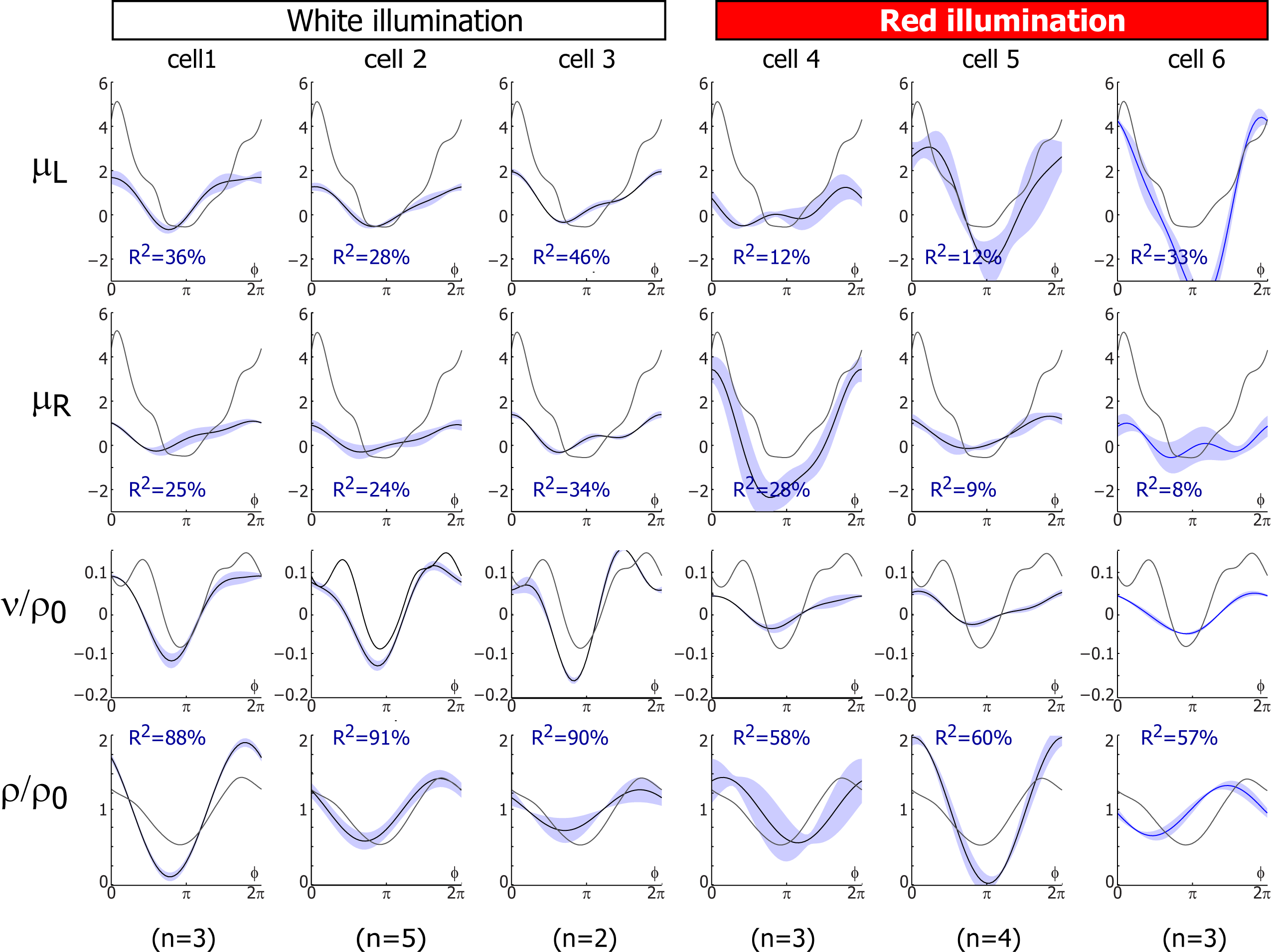
Figure S7: Experimental fits for the coupling functions $\mu$, $\nu$, and $\rho$ introduced in eqns. 2-4 (blue curves, shaded regions indicate mean$\pm$s.e.) and theoretical predictions (black). The coupling functions $\mu$, $\nu$, and $\rho$ relate flagellar beating and cell body yawing. Fitting results are shown for 6 different cells illuminated by either white or red light as indicated. For each cell, we employed $n$ fits using $n$ non-overlapping time series of duration $0.4-0.5\,\mathrm{s}$ with $n$ as indicated. The blue curves represent the average of the fitted coupling functions for the $n$ fits; the averaged coefficient of determination $R^{2}$ is stated.

We reconstructed the coupling functions $\mu(\varphi)$ and $\nu(\varphi)$ between beating and yawing from experimental data using the theoretical framework developed in the previous section. In brief, (1) we extracted the instantaneous yawing rate $\dot{\alpha}$ and flagellar phase speeds $\dot{\varphi}_{L}$ and $\dot{\varphi}_{R}$ from high-speed videos of swimming Chlamydomonas cells, (2) we represented the coupling functions by a truncated Fourier series, and (3) we obtained the unknown Fourier coefficients by linear regression using equations 2-4. The high temporal resolution of our imaging enabled us to accurately determine phase speeds as time-derivatives of flagellar phase angle data. Figure 5B displays averaged coupling functions obtained by fitting for a typical Chlamydomonas cell. We find a significant coupling between flagellar phase speeds and yawing rates, which are in good qualitative agreement with the theoretical predictions. Figure S7 in the SI shows fits for 5 more cells.

For the experimental conditions used, we commonly observed cells that displayed a large frequency mismatch between the two flagella. In the cells selected for analysis, this frequency mismatch exceeded $30\%$. This large frequency mismatch caused flagellar phase drift, which resulted in pronounced cell body yawing and enabled us to accurately measure the coupling of yawing and flagellar beating. Experiments were done using either white light illumination, which gave maximal image quality, or red light illumination, which reduces a possible phototactic stimulation of the cells.

The observed modulation of flagellar phase speed according to the rate of yawing is consistent with a force-velocity dependence of flagellar beating, for which the speed of the beat decreases, if the hydrodynamic load increases. We propose that a similar load characteristic of the flagellar beat holds also in cases of small frequency mismatch, where it allows for flagellar synchronization.

II Conclusion and Outlook

We have presented a theory on the hydrodynamic coupling underlying flagellar synchronization in swimming Chlamydomonas cells. We have shown that direct hydrodynamic interactions between the two flagella as considered in refs. Gueron:1999 ; Vilfan:2006 ; Niedermayer:2008 give only a minor contribution to the computed synchronization strength and are unlikely to account for the rapid synchronization observed in experiments Ruffer:1985a ; Ruffer:1998a ; Polin:2009 ; Goldstein:2009 . In contrast, rotational motion of the swimmer caused by asynchronous beating imparts different hydrodynamic friction forces on the two flagella, which rapidly brings them back in tune: Chlamydomonas rocks to get into synchrony.

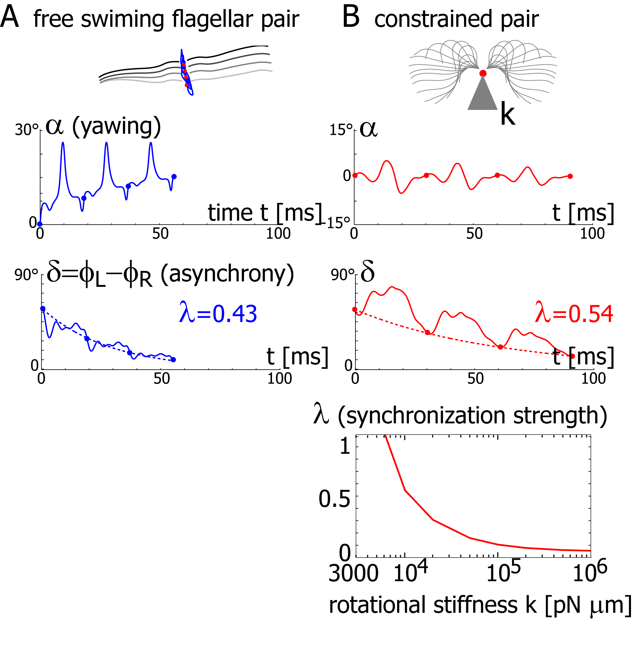
Figure S8: Theory of flagellar synchronization for an isolated flagellar pair. Inspired by experiments by Hyams et al. Hyams:1975 reporting synchronization in isolated flagellar pairs, we computed the swimming and synchronization behavior of a flagellar pair with cell body removed. For the computations, we used flagellar shapes and flagellar driving forces $Q_{j}(\varphi)$, $j=L,R$, determined from an intact cell, see figure 1. A. For a free swimming flagellar pair, we observe a characteristic yawing motion of the flagellar pair characterized by $\alpha(t)$, if the two flagella are initially out of synchrony. The flagellar phase difference $\delta$ is found to decrease with time (solid line), approximately following an exponential decay (dotted line). This implies that the in-phase synchronized state is stable with respect to perturbations. Each completion of a full beat cycle of the left flagellum is marked by a dot. B. To mimic experiments where external forces constrain the motion of the flagellar pair, we simulated the idealized case of a pair that cannot translate, while yawing of the pair is constricted by an elastic restoring torque $Q_{\alpha}=-k\alpha$ that acts at the basal apparatus (red dot). As in the case of a free-swimming pair, the flagellar phase difference $\delta$ decays with time, indicating stable synchronization. In the case of a constrained cell, the synchronization strength $\lambda$ strongly depends on the clamping stiffness $k$. Parameters: $2\pi/\omega_{0}=30\,\mathrm{ms}$, $k=10^{4}\,\mathrm{pN}\,\mu\mathrm{m/rad}$. To enhance numerical stability, we added a small constant $\kappa=10\,\mathrm{pN}\,\mu\mathrm{m}\,\mathrm{ms}$ to the flagellar friction coefficients, $\Gamma_{jj}(\varphi_{L},\varphi_{R})$, $j=L,R$, which corresponds to internal dissipation Friedrich:2012c .

Using high-speed tracking experiments, we could confirm the two-way coupling between flagellar beating and cell body yawing predicted by our theory. The striking reproducibility of our fits for the corresponding coupling functions and their favorable comparison to our theory is highly suggestive for a regulation of flagellar phase speed by hydrodynamic friction forces that depends on rotational motion. Thus, coupling of flagellar beating and cell body yawing provides a strong candidate for the mechanism that underlies flagellar synchronization of swimming Chlamydomonas cells. A similar mechanism may account for synchronization in isolated flagellar pairs Hyams:1975 , see figure S8.

To explain a previously observed synchronization for cells held in a micropipette Ruffer:1998a ; Polin:2009 ; Goldstein:2009 , we propose a finite clamping compliance that still allows for residual cell body yawing with an amplitude of a few degrees, which is sufficient for rapid synchronization. Alternatively, a compliant basal anchorage of the flagellar pair or bending deformations of the elastic cell body would allow for flagellar synchronization by a completely analogous mechanism. The simple theory for biflagellar synchronization by rotational motion presented in this manuscript (equations 2-4) is generic and applies also to the pivoting motion of an elastically anchored flagellar pair as shown in the Supporting Information. From the observed value $\lambda=0.3$ for the synchronization strength in clamped cells Goldstein:2009 , we estimate a rotational stiffness of $k\sim 10^{4}\,\mathrm{pN}\,{\mu\mathrm{m}}$ for either of these two cases.

Finally, the coupling of two phase oscillators by a third degree of freedom, in this case rotational motion, could allow for synchronization also in other contexts. For example, one may consider that synchronization in ciliar arrays Sanderson:1981 is mediated by an elastic coupling through the matrix with elastic deformations playing the role of the third degree of freedom.

III Hydrodynamic computation of swimming Chlamydomonas

We represent a Chlamydomonas cell by an ensemble of $300$ spheres of radius $a=0.25\,{\mu\mathrm{m}}$, see Figure 2A, and use a freely available hydrodynamic library based on a Cartesian multipole expansion technique Hinsen:1995 to compute the grand hydrodynamic friction matrix $\mathrm{G}$ Happel:hydro for this ensemble of spheres. We assume a rigid cell body, and hence that the spheres constituting the cell body move as a rigid unit, which results in $n=2\cdot 14+1$ independently moving objects. The matrix $\mathrm{G}$ has dimensions $6n\times 6n$ and relates the components of the translational and rotational velocities, $\mathrm{v}_{i}$ and $\Omega_{i}$, of each of the $n$ objects to the hydrodynamic friction forces and torques, $\mathrm{F}_{j}$ and $\mathrm{T}_{j}$, exerted by the $j$-th object on the fluid, $(F_{1x},F_{1y},F_{1z},T_{1x},T_{1y},T_{1z},F_{2x},F_{2y},\ldots,T_{ny},T_{nz})=\mathrm{G}\dot{\mathrm{q}}_{0}$ with $\dot{\mathrm{q}}_{0}=(v_{1x},v_{1y},v_{1z},\Omega_{1x},\Omega_{1y},\Omega_{1z},v_{2x},v_{2y},\ldots,\Omega_{ny},\Omega_{nz})$. Figure 2C,D shows the sub-matrix $G_{ij,yy}=G_{6i-4,6j-4}$, which relates $y$-components of velocities and $y$-components of hydrodynamic forces. The reduced friction matrix $\Gamma$ for a set of $m$ effective degrees of freedom $q$ is computed from $\mathrm{G}$ as $\Gamma=\mathrm{L}^{T}\mathrm{G}\mathrm{L}$ with $6n\times m$ transformation matrix $L_{ij}=\partial{\dot{q}_{0,i}}/\partial{\dot{q}_{j}}$, where $\mathrm{q}=(x,y,\alpha,\varphi_{L},\varphi_{R})$ Friedrich:2012c . Initial tests confirmed that the friction matrix of only the cell body gave practically the same result as the analytic solution for the enveloping spheroid; similarly the computed friction matrix of only a single flagellum matched the prediction of resistive force theory Happel:hydro .

IV Imaging Chlamydomonas swimming in a shallow observation chamber

Cell Culture: Chlamydomonas reinhardtii cells (CC-125 wild type mt+ 137c, R.P. Levine via N.W. Gillham, 1968) were grown in 300 ml TAP+P buffer Gorman:1965 (with 4 x phosphate) at $24^{\circ}$ C for 2 days under conditions of constant illumination (2x75 W, fluorescent bulb) and constant air bubbling to a final density of $10^{6}$ cells/ml.

High Speed Video Microscopy: An assay chamber was made of pre-cleaned glass and sealed using Valap, a 1:1:1 mixture of lanolin, paraffin, and petroleum jelly, heated to $70^{\circ}\,\mathrm{C}$. The surface of that chamber was blocked using casein solution (solution of casein from bovine milk 2 mg/ml, for 10 min) prior to the experiment. Single, non interacting cells were visualized using phase contrast microscopy set up on a Zeiss Axiovert 100 TV Microscope using a 63x Plan-Apochromat NA1.4 PH3 oil lens in combination with an 1.6x tube lens and an oil phase-contrast condenser NA 1.4. The sample was illuminated using a 100 W Tungsten lamp. For red-light imaging, an e-beam driven luminescent light pipe (Lumencor, Beaverton, USA) with spectral range of 640-657 nm and power of 75 mW was used. The sample temperature was kept constant at $24^{\circ}\,\mathrm{C}$ using an objective heater (Chromaphor, Oberhausen, Germany). For image acquisition, an EoSens Cmos high-speed camera was used. Videos were acquired at a rate of 1000 fps with exposure times of 1 ms (white light) and 0.6 ms (red light). Finally, cell positions and flagellar shapes were tracked using custom-build Matlab software, see SI for details.

V Figures

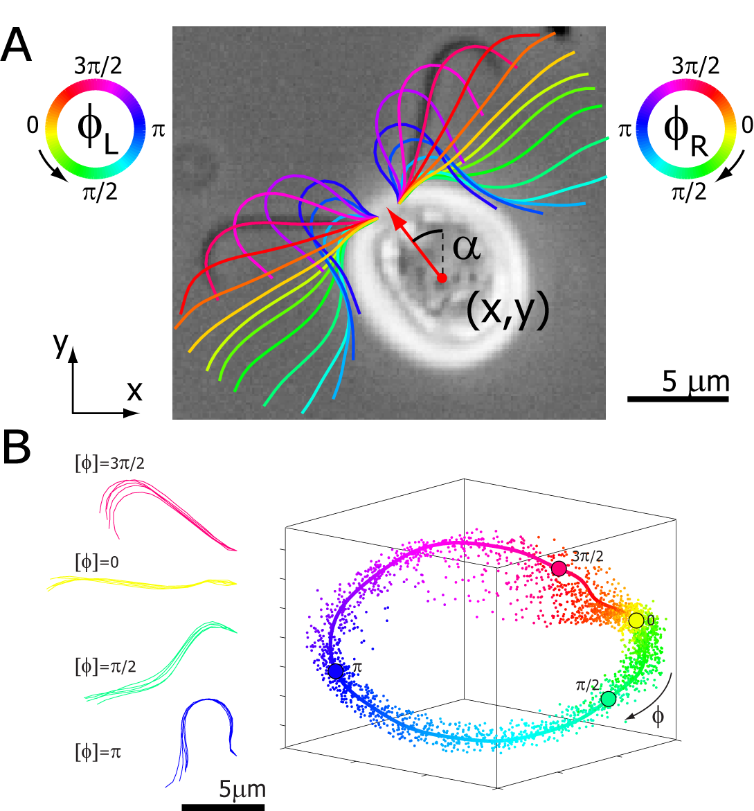
Figure 1: Five degrees of freedom for Chlamydomonas. A. In our experiments, conducted in shallow observation chambers, Chlamydomonas cells swim in a plane. At each time, the position and orientation of the cell body is characterized by its center position $(x,y)$ and the angle $\alpha$ of its long axis with respect to the laboratory frame. The beating of each flagellum is characterized by a single periodic phase variable, $\varphi_{L}$ and $\varphi_{R}$ for the left and right flagellum, respectively. The flagellar shapes shown in different colors were tracked from high-speed recordings and correspond to a time-difference of $2\,\mathrm{ms}$. This beat pattern was used for all computations. B. Binning of tracked flagellar shapes according to shape similarity defines a flagellar phase angle as shown on the left. More precisely, we employed a nonlinear dimensionality reduction technique as specified in the Supporting Information to represent each tracked planar flagellar shape as a point in an abstract shape space. This representation reveals the periodicity of the flagellar beat and supports our description of the flagellar beat as a fixed sequence of flagellar shapes parameterized by a single phase variable $\varphi$.

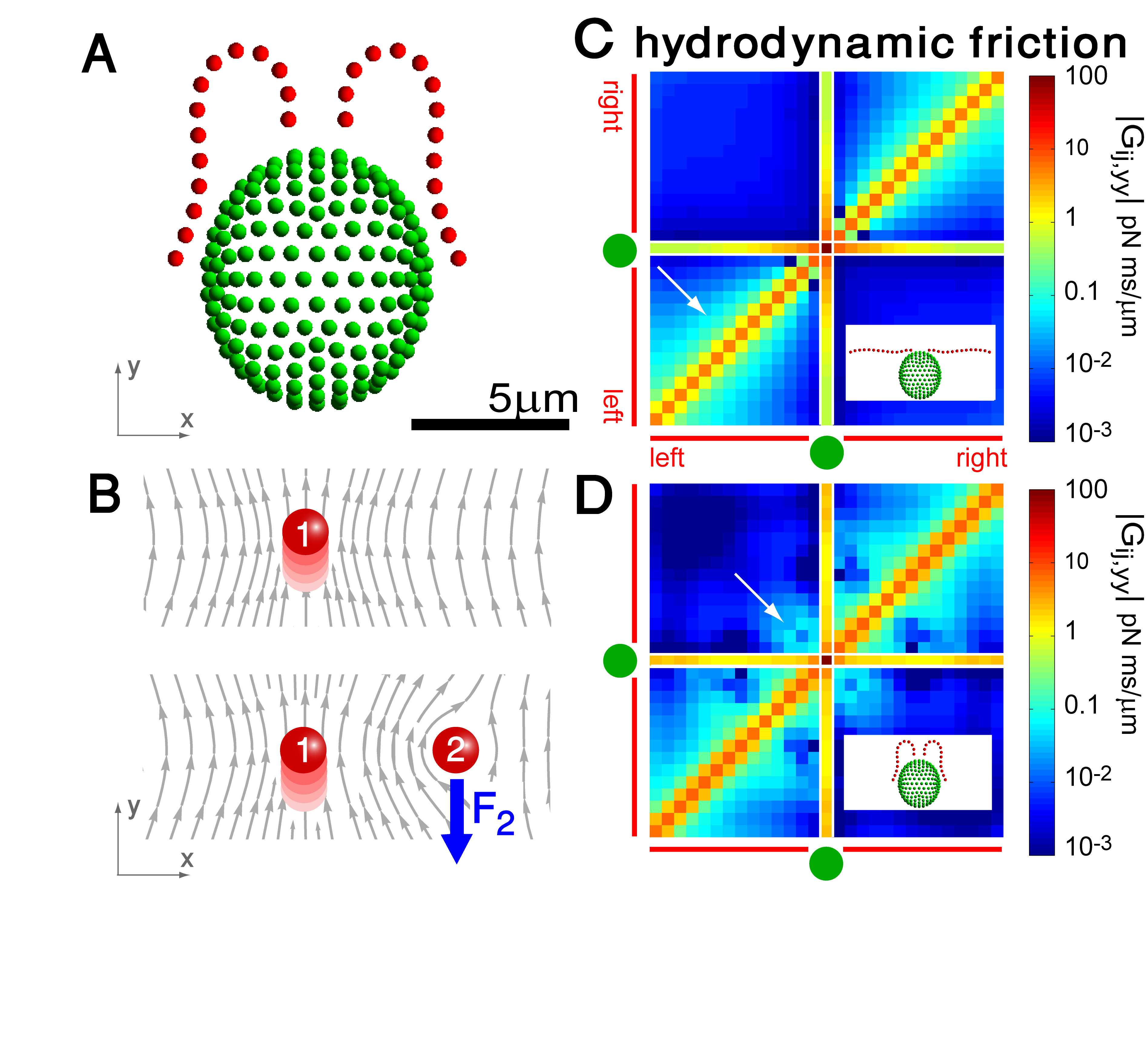
Figure 2: Hydrodynamic interactions between the two flagella are weak. A. Model Chlamydomonas cell represented by an ensemble of $300$ spheres used to compute hydrodynamic friction forces at low Reynolds numbers. In our calculations, the model cell was assumed to be far from any surfaces. B. Illustration of hydrodynamic interactions between spheres. A single sphere (labeled $1$) moving with velocity $v_{1y}>0$ along the $y$-axis will drag fluid alongside and thus exert a total hydrodynamic friction force $F_{1y}=G_{11,yy}v_{1y}>0$ on the fluid. If a second sphere (labeled $2$) is held fixed close to the first one, it will locally slow down this fluid flow. The force $\mathrm{F}_{2}$ required to hold the second sphere equals the force exerted by this sphere on the fluid; its $y$-component $F_{2y}=G_{21,yy}v_{1y}<0$ defines a friction coefficient $G_{21,yy}$ that characterizes hydrodynamic interactions between the two spheres. C. Hydrodynamic interactions between different parts of the model cell. Analogous to panel B, one defines a matrix $G_{ij,yy}$ of hydrodynamic friction coefficients for the ensemble of $2\cdot 14$ flagellar spheres and the rigid sphere cluster constituting the cell body that together represent a Chlamydomonas cell (inset). Each column of the color coded matrix shows the magnitude of hydrodynamic friction exerted by a flagellar sphere (or the cell body), if a single sphere or the cell body is moved parallel to the long cell body axis. Off-diagonal entries characterize hydrodynamic interactions, which are particularly pronounced along a single flagellum (white arrow), or between one flagellum and the cell body (central column). Hydrodynamic interactions between the two flagella are very weak and partly screened by the cell body. D. Same as in panel C, but for a recovery stroke configuration. There are weak hydrodynamic interactions between the proximal segments of the two flagella (white arrow). All friction coefficients shown scale with the viscosity of the fluid, which was taken as the viscosity of water at $20^{\circ}$ Celsius, $\eta=1\,\mathrm{pN\,ms}/{\mu\mathrm{m}}^{2}$.

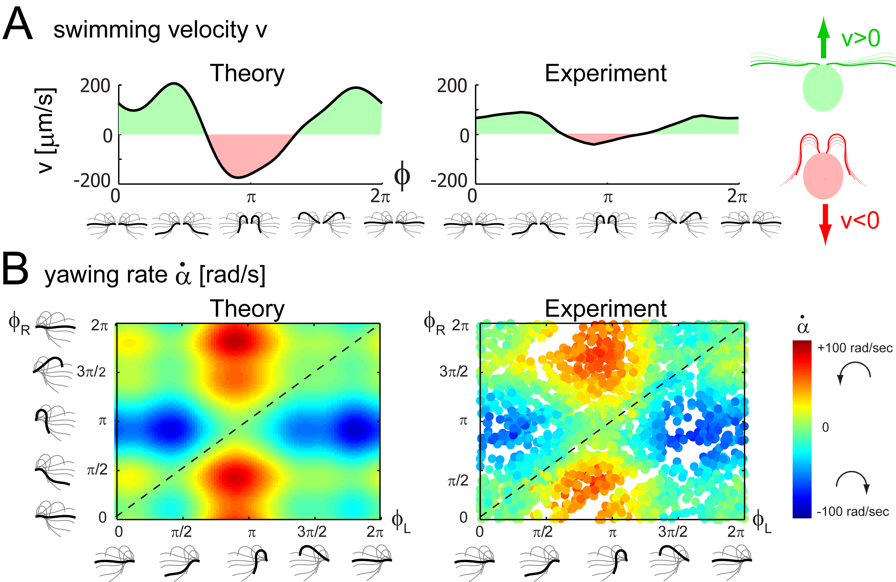
Figure 3: A. For synchronized flagellar beating, we compute saltatory forward swimming with positive instantaneous velocity during effective stroke beating, and a backward motion during the recovery stroke (left panel); this behavior is summarized by cartoon drawings to the very right. A typical experimental velocity profile of a Chlamydomonas cell in a shallow observation chamber measured during a cycle of synchronized beating is shown for comparison in the middle panel. B. Flagellar asynchrony causes cell body yawing, both in theory and experiment. Shown is the instantaneous rotation rate $\dot{\alpha}$ of the cell body in color code as a function of the respective phase of the two flagella. For in-phase synchronized flagellar beating (dashed line), the cell body does not rotate (green). For out-of-phase flagellar beating, however, we find significant cell body rocking (blue: clockwise, red: counter-clockwise).

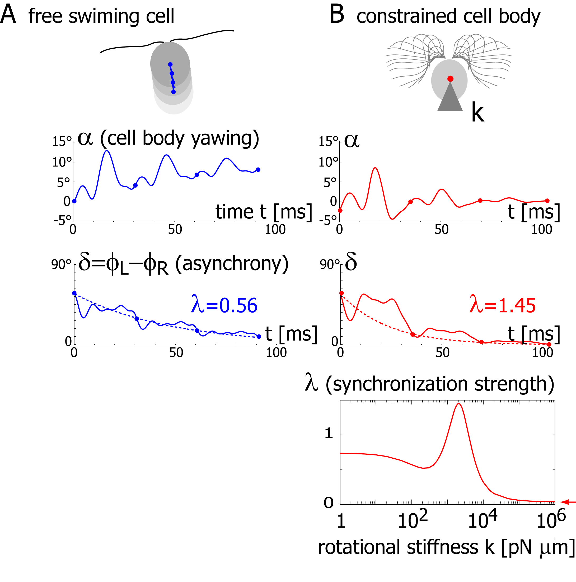
Figure 4: Flagellar synchronization by cell body yawing. A. For a free swimming cell (top panel), the equation of motion 1 predicts a yawing motion of the cell body characterized by $\alpha(t)$ if the two flagella are initially out of synchrony (middle panel). The flagellar phase difference $\delta$ is found to decrease with time (lower panel, solid line), approximately following an exponential decay $\sim\exp(-\lambda t/T)$ (dotted line), where $T$ is the period of the flagellar beat and $\lambda$ defines a dimensionless synchronization strength. Thus, in-phase synchronized beating is stable with respect to perturbations. Dots mark the completion of a full beat cycle of the left flagellum. B. To mimic experiments where external forces constrain cell motion, we simulated the idealized case of a cell that cannot translate, while cell body yawing is constricted by an elastic restoring torque $Q_{\alpha}=-k\alpha$ that acts at the cell body center (upper panel). Again, the two flagella synchronize ($3^{\mathrm{rd}}$ panel) with a synchronization strength $\lambda$ that can become even larger than in the case of a free swimming as shown here for $k=2\cdot 10^{3}\,\mathrm{pN}\,\mu\mathrm{m}$, which is close to the rotational stiffness for which the synchronization strength $\lambda$ is maximal (lowest panel). For very large clamping stiffness $k$, the cell body cannot move and the synchronization strength $\lambda$ attenuates to a basal value $\lambda\approx 0.03$, which arises solely from direct hydrodynamic interactions between the two flagella (arrow). Parameters: $2\pi/\omega_{0}=30\,\mathrm{ms}$.

VI Supporting Information

VI.1 Image analysis

High-speed movies were analyzed using custom-made Matlab software (The MathWorks Inc., Natnick, MA, USA); our image analysis pipeline is illustrated in figure S1: In a first step, estimates for position and orientation of the cell body in a movie frame were obtained by a cross-correlation analysis using rotated template images. In a second step, these position and orientation estimates were refined by tracking the bright phase halo surrounding the cell. The first and second area moments of the cell rim provide accurate estimates for the center of the cell body and its long orientation axis: While the tracking precision of the first step amounts to $<500\mathrm{nm}$ for the position and a few degrees for the orientation, these values are reduced to $<50\mathrm{nm}$ and $<0.5^{\circ}$ after the second step, respectively. Special care was taken to reduce any potential bias of the flagellar phase on the cell body tracking; for example, the cell rim close to the flagellar bases was obtained by interpolation instead of direct tracking. The flagellar base is visible as a continuous, parabola-shaped curve that connects the proximal ends of the two flagella; tracking of this flagellar base was done by a combination of line-scans and local fitting of a Gaussian line model (step 3). Flagella were tracked by advancing along their length using exploratory line-scans in a successive manner (step 4). Flagellar tracking can be refined by local fitting of a Gaussian line model. A movie consisting of thousand frames can be analyzed in an automated manner within 10 hours on a standard PC. Movies from red light illumination conditions were of lower quality and required manual correction of the automated tracking results for each frame.

VI.2 Flagellar shape analysis

We employ a non-linear dimension reduction technique to represent tracked flagellar shapes as points in a low-dimensional abstract shape space. In a first step, smoothed tracked flagellar shapes corresponding to one cycle of synchronized flagellar beating (shown in figure 1A) were used to define the basis of the shape space. Flagellar shapes can be conveniently represented with respect to the material frame of the cell using a tangent angle representation Riedel:2007 ; Friedrich:2010 . In terms of this tangent angle $\theta(s)$, the $x(s)$ and $y(s)$ coordinates of the flagellar midline as functions of arclength $s$ along the flagellum can be expressed as

$$x(s)=x(0)+\int_{0}^{s}d\xi\,\cos[\alpha+\theta(\xi)]\text{ and }y(s)=y(0)+\int_{0}^{s}d\xi\,\sin[\alpha+\theta(\xi)].$$ (S1)

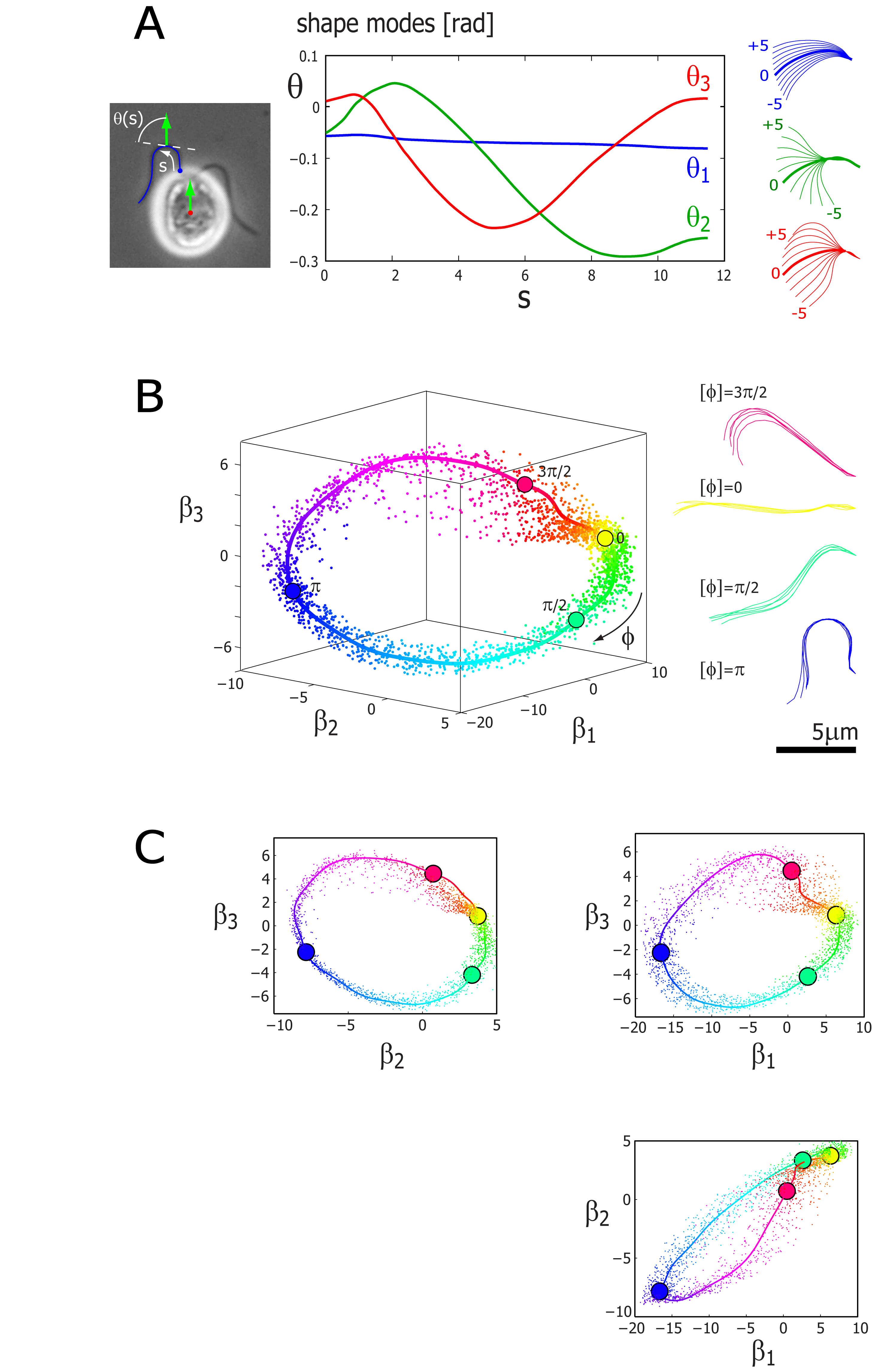
Figure S2: We represent a single flagellar shape by $n=3$ shape coefficients as a point in an abstract shape space that is spanned by $3$ principal shape modes. A. The principal shape modes were determined by employing a kernel principal component analysis (PCA) to the tangent angle representation $\theta(s)$ of smoothed flagellar shapes that were tracked from the left flagellum of cell no. 2 during one beat cycle of synchronized flagellar beating. From the PCA, we obtained three dominant shape modes with respective tangent angle representations $\theta_{1}(s)$, $\theta_{2}(s)$, $\theta_{3}(s)$ as shown. Together, these principal shape modes account for $97\%$ of the variance of this tangent angle data set. For sake of illustration, exemplary flagellar shapes corresponding to the superposition of the mean flagellar shape and just one shape mode with tangent angle $\overline{\theta}(s)+\beta_{i}\theta_{i}(s)$, $i=1,2,3$ are shown to the right ($-5\leq\beta_{i}\leq 5$). B. Each tracked flagellar shape from one flagellum can be represented by a single point in an abstract shape space that is spanned by the three principal shape modes. More specifically, the coordinates $(\beta_{1},\beta_{2},\beta_{3})$ of this point are obtained by approximating the tracked flagellar shape by a superposition of a previously computed mean flagellar shape and the three principal shape modes, see equation S2. The set of flagellar shapes from an entire experimental movie thus corresponds to a point cloud. This point cloud scatters around a closed curve (solid line), which reflects the periodic nature of the flagellar beat. This closed curve has been obtained by a simple fit to the point cloud of flagellar shapes and can be considered as a limit cycle of flagellar beating. Deviations from this limit cycle measure the variability of the flagellar beat. We can use this representation to define a distinct flagellar phase angle $\varphi$ (modulo $2\pi$) for each tracked flagellar shape as indicated by the color code by mapping each flagellar shape onto the limit cycle. A time-series of flagellar shapes thus yields a time-series of the flagellar phase angle $\varphi(t)$. As an illustration of this assignment, superpositions of flagellar shapes are shown to the right, each of which correspond to flagellar shapes that were assigned the same flagellar phase modulo $2\pi$. C. Two-dimensional projections corresponding to the three-dimensional shape space representation in panel B.

Here, $\alpha$ is the orientation angle of the long axis of the cell body (figure 1A), which implies that $\theta(\xi)$ characterizes flagellar shapes with respect to a material frame of the cell body. By averaging the tangent angle profiles $\theta(s,t)$ over a full beat cycle, we define a time-averaged flagellar shape characterized by a tangent angle $\overline{\theta}(s)$. To characterize variations from this mean flagellar shape, we employed a kernel principal component analysis (PCA) Scholkopf:kernel . The kernel used to compute the Gram matrix $\mathrm{D}$ for the kernel PCA must account for the $2\pi$-periodicity of the tangent angle data and was taken as $D_{ij}=\int_{0}^{L}ds\,\cos[\theta(s,t_{i})-\theta(s,t_{j})]$. The first three shape eigenmodes account for 97% of the spectrum of $\mathrm{D}$ and are shown in figure S2A. The relative contributions to the spectrum read $67\%$ (first mode), $18\%$ (second mode), $12\%$ (third mode). While the first mode $\theta_{1}(s)$ (blue) describes nearly uniform bending of the flagellum, the second mode $\theta_{2}(s)$ (green) and the third mode $\theta_{3}(s)$ (red) together comprise the components of a traveling bending wave.

Next, any flagellar shape can be projected onto the shape space spanned by these three shape modes: Given a flagellar midline with coordinates $x(s)$ and $y(s)$, we seek the optimal approximating shape with coordinates $\hat{x}(s)$, $\hat{y}(s)$ whose tangent angle $\hat{\theta}(s)$ is a linear combination of the fundamental shape modes

$$\hat{\theta}(s)=\overline{\theta}(s)+\beta_{1}\theta_{1}(s)+\beta_{2}\theta_{2}(s)+\beta_{3}\theta_{3}(s).$$ (S2)

The coefficients $\beta_{1}$, $\beta_{2}$, $\beta_{3}$ are obtained by a non-linear fit that minimizes the squared Euclidean distance $\int_{0}^{L^{\prime}}ds|x(s)-\hat{x}(s)|^{2}+|y(s)-\hat{y}(s)|^{2}$. This procedure is robust and works even if flagellar shapes could only be tracked partially with tracked length $L^{\prime}$ shorter than the total flagellar length $L$. Note that for non-smoothed flagellar shapes, the tangent angle representations can be noisy and are thus less suitable for fitting as compared to $x,y$ coordinates.

A time sequence of tracked flagellar shapes thus results in a point cloud in the shape space parametrized by the shape mode coefficients $\beta_{1}$, $\beta_{2}$, $\beta_{3}$. We fitted a closed curve to the torus-like point cloud, see the solid line in figure S2B. This closed curve represents a limit cycle of periodic flagellar beating. Each tracked flagellar shape can be assigned the ‘closest’ point on this limit cycle, i.e. the point for which the corresponding flagellar shape has minimal Euclidean distance. By choosing a phase angle parametrization for the limit cycle, the phase angle of each flagellar shape is determined modulo $2\pi$. A time-series of flagellar shapes thus yields a time-series of the flagellar phase angle $\varphi(t)$. The phase angle parametrization of the limit cycle had been chosen such that the flagellar phase angle $\varphi$ and its time derivative are not correlated. Finally, the zero point $\varphi=0$ was chosen such that the corresponding flagellar shape was nearly straight and perpendicular to the long cell axis.

VI.3 Computation of hydrodynamic friction forces

For our hydrodynamic computations, we represented a Chlamydomonas cell by an ensemble of $N=300$ equally sized spheres of radius $a=0.25\,{\mu\mathrm{m}}$. The cell body was chosen spheroidal and is represented by $272$ spheres that are arranged in a symmetric fashion to retain mirror symmetries. Each flagellum is represented by a chain of $14$ spheres that are aligned along a flagellar midline with equidistant spacing. The shapes of the flagellar midlines depend on respective phase angles $\varphi_{L}$ and $\varphi_{R}$ for the left and right flagellum. These flagellar shapes were taken from experiment for one full period of synchronized beating and are shown in figure 1A. We assume that the $272$ spheres constituting the cell body move as a rigid sphere cluster. Each of the flagellar spheres represents a cluster with just one sphere, which results in a total of $n=2\cdot 14+1=29$ sphere clusters. We then computed the $6n\times 6n$ grand hydrodynamic friction matrix $\mathrm{G}$ for this ensemble of $n$ spheres clusters using a freely available hydrodynamic library based on a Cartesian multipole expansion technique Hinsen:1995 . Recall that the grand hydrodynamic friction matrix $\mathrm{G}$ relates the forces and torques exerted by the $6n$ sphere clusters to their translational and rotational velocities Happel:hydro

$$\mathrm{P}_{0}=\mathrm{G}\cdot\dot{\mathrm{q}}_{0}.$$ (S3)

Here, $\dot{\mathrm{q}}_{0}$ denotes a $6n$-vector that combines the translational and rotational velocity components of the $n$ sphere clusters,

$$\dot{\mathrm{q}}_{0}=(v_{1x},v_{1y},v_{1z},\omega_{1x},\omega_{1y},\omega_{1z},\ldots,\omega_{nz}),$$ (S4)

while the $6n$-vector $\mathrm{P}_{0}$ combines the components of the resultant hydrodynamic friction forces and torques,

$$\mathrm{P}_{0}=(F_{1x},F_{1y},F_{1z},T^{\prime}_{1x},T^{\prime}_{1y},T^{\prime}_{1z},\ldots,T^{\prime}_{nz}).$$ (S5)

(Primed torques represent torques with respect to the center of the respective sphere cluster.) Figure 2C,D in the main text shows a sub-matrix of the grand friction matrix, which was defined as $G_{ij,yy}=G_{6i-4,6j-4}$, $i,j=1,\ldots,n$. In this figure, it was assumed that the long cell body axis is aligned with the $y$-axis of the laboratory frame, i.e. $\alpha=0$, which implies that the sub-matrix relates motion in the direction of the long cell axis and the hydrodynamic force components projected on this axis.

For our hydrodynamic computations, the multipole expansion order was chosen as $3$. An estimate for the accuracy of our computation could be obtained by increasing the expansion order parameter, which changed the computed friction coefficients by less than $1\,\%$. Initial tests confirmed that the friction matrix of only the cell body gave practically the same result as the analytic solution for the enveloping spheroid Perrin:1934 ; similarly the computed friction matrix of only a single flagellum matched the prediction of resistive force theory Gray:1955b assuming a flagellar radius equal to the sphere radius. Note that the precise value of the flagellar radius is expected to affect hydrodynamic friction coefficients only as a logarithmic correction Brennen:1977 .

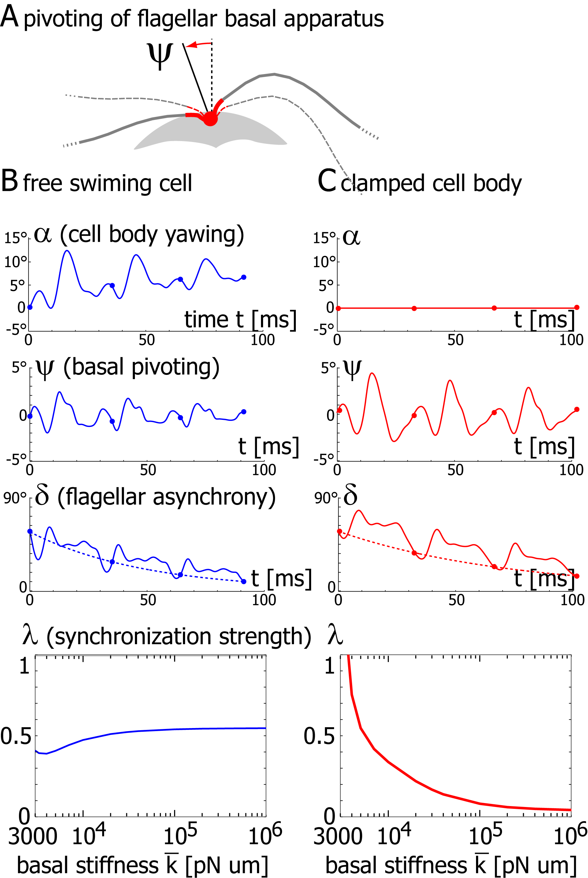
Figure S9: Theory of flagellar synchronization by basal pivoting. A. We consider the possibility of an elastically anchored flagellar basal apparatus (red), which allows for pivoting of the basal apparatus (solid lines) by an angle $\psi$ from its symmetric reference configuration (dashed). B. For a free swimming cell, the equation of motion S17 predicts both a yawing motion of the cell characterized by $\alpha(t)$ and a pivoting motion of the flagellar base characterized by $\psi(t)$, if the two flagella are initially out of synchrony. The flagellar phase differences $\delta$ is found to decrease with time (solid line), approximately following an exponential decay (dotted line). This implies that the in-phase synchronized state is stable with respect to perturbations. Each completion of a full beat cycle of the left flagellum is marked by a dot. The synchronization behavior in the case of an elastically anchored flagellar basal apparatus is nearly identical to the case of a stiff anchorage as shown in the main text in figure 4. The lowest panel shows typical amplitudes of basal pivoting ($\delta\psi$, solid line) and cell body yawing ($\delta\alpha$, dashed) as a function of basal stiffness $\overline{k}$. Amplitudes were determined as half the range of variation during one beat cycle for an initial phase difference of $\delta(0)=\pi/2$. C. For a clamped cell that can neither translate nor rotate, the flagellar apparatus can still pivot and will do so if the two flagella are initially out of phase. As in the case of a free-swimming cell, the flagellar phase difference $\delta$ decays with time, indicating stable synchronization. In the case of a clamped cell, the synchronization strength $\lambda$ strongly depends on the stiffness $\overline{k}$ of the elastic anchorage of the basal flagellar apparatus, which sets the amplitude of basal pivoting. Parameters: $2\pi/\omega_{0}=30\,\mathrm{ms}$, $\overline{k}=10^{4}\,\mathrm{pN}\,\mu\mathrm{m/rad}$.

Below, we consider an extension of the theoretical description given in the main text that additionally considers the possibility of an elastically anchored flagellar base, which allows for pivoting of the flagellar basal apparatus, see figure S9. In this case, the flagellar midlines were rotated by an angle $\psi$.

A set of 2400 pre-computed configurations was then used to construct a spline-based lookup-table of the (reduced) hydrodynamic friction matrix as a function of the degrees of freedom $\varphi_{L}$, $\varphi_{R}$ and $\psi$. The interpolation error was confirmed to be on the order of $1\,\%$ or less. This lookup-table was then used for the numerical integration of the (stiff) equations of motion 1 and S17.

VI.4 Generalized hydrodynamic friction forces

We employ the framework of Lagrangian mechanics of dissipative systems Goldstein:mechanics to define generalized hydrodynamic friction forces and derive an equation of motion for the effective degrees of freedom in our theoretical description of Chlamydomonas swimming and synchronization. The $6n$ degrees of freedom $\mathrm{q}_{0}$ for the $n$ sphere clusters used in our hydrodynamic computations are enslaved by the 5 effective degrees of freedom in our coarse-grained theory, see figure 1. Below, one more degree of freedom $\psi$ is introduced to characterize pivoting of an elastically anchored flagellar basal apparatus. We thus have

$$\mathrm{q}_{0}=\mathrm{q}_{0}(\mathrm{q}),$$ (S6)

where we introduced the $6$-component vector $\mathrm{q}=(x,y,\alpha,\varphi_{L},\varphi_{R},\psi)$ that comprises the $6$ effective degrees of freedom. The reduced $6\times 6$ hydrodynamic friction matrix $\Gamma$ for these $6$ effective degrees of freedom can be computed from the grand hydrodynamic friction matrix $\mathrm{G}$ as

$$\Gamma=\mathrm{L}^{T}\cdot\mathrm{G}\cdot\mathrm{L}$$ (S7)

with a $6n\times 6$ transformation matrix $\mathrm{L}$ given by Friedrich:2012c

$$L_{ij}=\partial{\dot{q}_{0,i}}/\partial{\dot{q}_{j}}.$$ (S8)

The rate of hydrodynamic dissipation can now be equivalently written as a quadratic function of either $\dot{\mathrm{q}}_{0}$ or $\dot{\mathrm{q}}$

$$\mathcal{R}=\dot{\mathrm{q}}_{0}^{T}\cdot\mathrm{G}\cdot\dot{\mathrm{q}}_{0}=\dot{\mathrm{q}}^{T}\cdot\Gamma\cdot\dot{\mathrm{q}}.$$ (S9)

The generalized hydrodynamic friction coefficients $\Gamma_{ij}$ are depicted in figure S3. In this context, generalized hydrodynamic friction forces can be defined as

$$P_{j}=\Gamma_{jx}\dot{x}+\Gamma_{jy}\dot{y}+\Gamma_{j\alpha}\dot{\alpha}+\Gamma_{jL}\dot{\varphi}_{L}+\Gamma_{jR}\dot{\varphi}_{R}+\Gamma_{j\psi}\dot{\psi},\quad j=x,y,\alpha,L,R,\psi.$$ (S10)

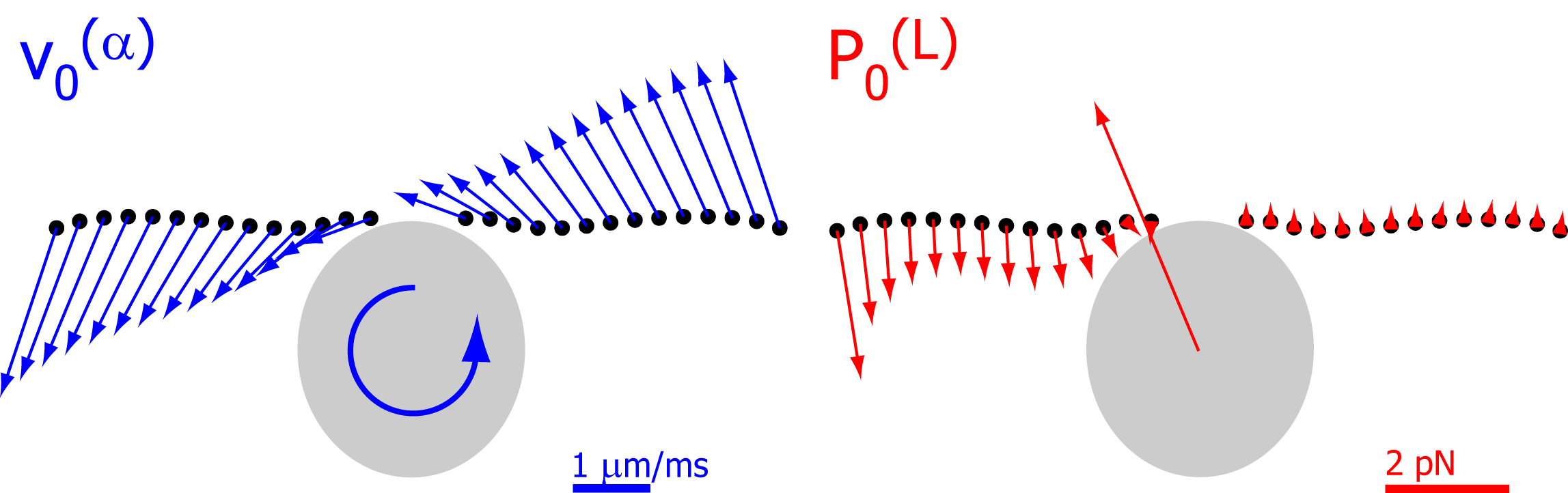
Figure S4: Coupling of cell body yawing and flagellar beating. (left) Translational velocities of the flagellar spheres used in our hydrodynamic computation associated with a pure yawing motion of the cell body with rate $\dot{\alpha}$. (right) Hydrodynamic friction forces exerted by the flagellar spheres (as well as by the cell body), if the left flagellum advances along its beat cycle with rate $\dot{\varphi}_{L}$. The generalized hydrodynamic friction coefficient $\Gamma_{\alpha L}$ that couples cell body yawing and beating of the left flagellum can be computed as a scalar product between the velocity profile resulting from yawing and the force profile resulting from flagellar beating and is found to be non-zero. Parameters: $\dot{\varphi}_{L}=\omega_{0}$, $\dot{\alpha}=0.2\omega_{0}$, $2\pi/\omega_{0}=30\,\mathrm{ms}$.

Interestingly, the generalized hydrodynamic friction force conjugated to one degree of freedom depends also on the rates of the change of the other degrees of freedom, which implies a coupling between the various degrees of freedom. This fact is illustrated by figure S4. Panel A depicts the translational velocities of the flagellar spheres caused by pure yawing of the cell body with rate $\dot{\alpha}$. This motion is characterized by a $6n$-vector of velocity components, $\dot{\mathrm{q}}_{0}^{(\alpha)}=\mathrm{L}\cdot(0,0,\dot{\alpha},0,0,0)^{T}$. Similarly, the beating of the left flagellum induces hydrodynamic friction forces as shown in figure S4B. The resultant force (and torque) components are combined in the $6n$-vector $\mathrm{P}_{0}^{(L)}=\mathrm{G}\cdot\mathrm{L}\cdot(0,0,0,\dot{\varphi}_{L},0,0)^{T}$. Figure S4 indicates that the scalar product $\dot{\mathrm{q}}_{0}^{(\alpha)}\cdot\mathrm{P}_{0}^{(L)}=\dot{\alpha}\Gamma_{\alpha L}\dot{\varphi}_{L}$ does not vanish, which implies a non-zero friction coefficient $\Gamma_{\alpha L}$ and thus a coupling between cell body yawing and flagellar beating.

In our theoretical description, the phase dynamics of the left flagellum, say, is governed by a balance of the generalized hydrodynamic friction force $P_{L}$ and an active driving force $Q_{L}$; similarly, $Q_{R}=P_{L}$ for the right flagellum. In the case of free swimming, force and torque balance imply $P_{x}=P_{y}=0$ and $P_{\alpha}=0$. Together with an equation for $P_{\psi}$, these equation allow to self-consistently solve for the rate of change $\dot{\mathrm{q}}$ of the $6$ degrees of freedom. If one degree of freedom were constrained, $q_{j}=0$, the corresponding force equation becomes void, since a constraining force $Q_{j}$ equal to $P_{j}$ then balances the generalized hydrodynamic friction force $P_{j}$ associated with this degree of freedom.

In general, the active driving forces $Q_{L}$ and $Q_{R}$ will depend on the flagellar phase. This phase-dependence is fully determined by the requirement that the flagellar phase speeds should be constant, $\dot{\varphi}_{j}=\omega_{0}$, in the case of synchronized flagellar beating with $\delta=0$. Here, $\omega_{0}$ denotes the angular frequency of synchronized flagellar beating. Explicitly, we find

$$Q_{L}(\varphi_{L})=\omega_{0}[\Gamma_{LL}(\varphi_{L},\varphi_{L})+\Gamma_{LR}(\varphi_{L},\varphi_{L})-2\Gamma^{2}_{Ly}(\varphi_{L},\varphi_{L})/\Gamma_{yy}(\varphi_{L},\varphi_{L})].$$ (S11)

An analogous expression holds for $Q_{R}(\varphi_{R})$. Note that the generalized active driving forces are conjugate to an angle, and therefore have the physical unit $\mathrm{pN}\,\mu\mathrm{m}/\mathrm{rad}$. These phase-dependent active driving forces can be written as potential forces $Q_{j}=-\partial U/\partial\varphi_{j}$, $j=L,R$, where the potential $U$ reads

$$U=-\int_{-\infty}^{\varphi_{L}}d\varphi_{L}\,Q_{L}(\varphi_{L})-\int_{-\infty}^{\varphi_{R}}d\varphi_{R}\,Q_{R}(\varphi_{R}).$$ (S12)

The potential $U$ continuously decreases with time, indicating the depletion of an internal energy store and the dissipation of energy into the fluid during flagellar swimming. The rate of hydrodynamic dissipation equals the rate at which potential energy is dissipated

$$\mathcal{R}=-\dot{U}=Q_{L}\dot{\varphi}_{L}+Q_{R}\dot{\varphi}_{R}.$$ (S13)

VI.5 Analytic expression for the flagellar synchronization strength

We present details on the derivation of equations 5 and 6 for the synchronization strength $\lambda$ in the case of the reduced equations of motion 2-4. We assume equal intrinsic beat frequencies, $\omega_{L}=\omega_{R}=\omega_{0}$ and a small initial phase difference, $0<\delta(0)\ll 1$. To leading order in $\delta$, we find relations that link the rotation rate $\dot{\alpha}$ and the rate $\dot{\delta}$ at which the phase difference changes,

$$k\alpha+\rho(\varphi,\varphi)\dot{\alpha} =-d[\nu(\varphi)\delta]/dt$$ (S14)

$$\dot{\delta} =-2\mu(\varphi)\dot{\alpha}.$$ (S15)

Here $\varphi\approx\omega_{0}t$ denotes the mean flagellar phase. The first equation describes how flagellar asynchrony causes a yawing motion of the cell body, while the second equation describes how this yawing motion then changes the flagellar phase difference. In the absence of any elastic constraint for yawing, $k=0$, we can solve for $\dot{\delta}$

$$(\rho-2\mu\nu)\dot{\delta}=2\mu\nu^{\prime}\omega_{0}\delta.$$ (S16)

Now, equation 5 follows from equation S16 using $\lambda=-\int_{0}^{T}dt\,\dot{\delta}/\delta$ and a variable transformation $\varphi(t)=\omega_{0}t+\mathcal{O}(\delta)$.

In the case of a very stiff elastic constraint with $k\gg\rho\omega_{0}$, we make use of the fact that variations of the phase difference $\delta$ during one beat cycle will be small compared to its mean value $\delta_{0}=\langle\delta\rangle$. As a consequence, equation S14 can be approximated as $k\alpha=-\nu^{\prime}\omega_{0}\delta_{0}$. Using this approximation and equation S15, equation 6 follows.

VI.6 Comparison of experiment and theory

We can compare instantaneous swimming velocities predicted by our hydrodynamic computation with experimental measurements and find favorable agreement, see figures 3 and S5. Note that wall effects present in our experiments, but not accounted for by our hydrodynamic computations, are expected to reduce translational velocities (but less so rotational velocities) Bayly:2011 . The hydrodynamic computations are based on a fixed flagellar beat pattern parametrized by a flagellar phase angle, which was obtained experimentally for one beat cycle with synchronized beating (shown in figure 1A). The good agreement between theoretical predictions and experimental measurements for the instantaneous swimming velocities further validate our reductionist description of the flagellar shape dynamics by just a single phase variable for each flagellum. Next, we tested the applicability of the reduced equations of motion eqs. 2-4 in the experimental situation. For this aim, we reconstructed the coupling functions $\mu(\varphi)$, $\nu(\varphi)$ and $\rho(\varphi)$ from experimental time series data for $\dot{\alpha}$, $\dot{\varphi}_{L}$, and $\dot{\varphi}_{R}$. The coupling functions were represented by truncated Fourier series and the unknown Fourier coefficients determined by a linear regression of equation 2, 3, or 4, respectively, see figure S6. Repeating this fitting procedure for data from 6 different cells gave consistent results, see S7. Moreover, the phase-dependence of the fitted coupling functions agrees qualitatively with our theoretical predictions. Note that our simple theory does not involve any adjustable parameters.

VI.7 An elastically anchored flagellar basal apparatus

In the main text, we had assumed for simplicity that the flagellar base is rigidly anchored to the cell body. While the proximal segments of the two flagella are tightly mechanical coupled with each other by so-called striated fibers to form the flagellar basal apparatus, the flagellar basal apparatus itself is only connected to an array of $16$ long microtubules spanning the cell Ringo:1967 . We now consider the possibility that this anchorage allows for some pivoting of the flagellar basal apparatus as a whole by an angle $\psi$, see figure S9A. In addition to the five degrees of freedom of Chlamydomonas beating and swimming considered in the main text (see figure 1), we now include this pivot angle $\psi$ as a $6^{\mathrm{th}}$ degree of freedom. The rate of hydrodynamic dissipation is now given by $\mathcal{R}=\dot{x}P_{x}+\dot{y}P_{y}+\dot{\alpha}P_{\alpha}+\dot{\varphi}_{L}P_{L}+\dot{\varphi}_{R}P_{R}+\dot{\psi}P_{\psi}$, with $P_{\psi}$ being the generalized hydrodynamic friction force conjugate to the pivot angle $\psi$. Assuming Hookean behavior for the elastic basal anchorage with rotational pivoting stiffness $\overline{k}$, we readily arrive at an equation of motion that reads in the case of free swimming

$$(\dot{x},\dot{y},\dot{\alpha},\dot{\varphi}_{L},\dot{\varphi}_{R},\dot{\psi})^{T}=\Gamma^{-1}(0,0,0,Q_{L},Q_{R},-\overline{k}\psi)^{T}.$$ (S17)

Figure S9B shows flagellar synchronization for a free swimming cell with elastically anchored flagellar base: Although some basal pivoting occurs as a result of flagellar asynchrony, the swimming and synchronization behavior is very similar to the case of a rigidly anchored flagellar base as shown in figure 4A. For a cell that can neither translate nor yaw, however, the situation is different, see figure S9C. We find strong flagellar synchronization provided the elastic stiffness $\overline{k}$ is not too large. Flagellar synchronization by basal pivoting is thus effective also for a fully clamped cell. In contrast, for a rigidly anchored flagellar base, the synchronization strength $\lambda$ would be relatively weak in this case, being due only to direct hydrodynamic interactions between the two flagella.

Flagellar synchronization by basal pivoting is conceptually very similar to synchronization by cell body yawing as discussed in the main text. In the case of a fully clamped cell, we can approximate the synchronization dynamics by virtually the same generic equation of motion as eqs. 2-4, when we substitute $\psi$ for $\alpha$

$$\dot{\varphi}_{L} =\omega_{0}-\overline{\mu}(\varphi_{L})\dot{\psi},$$ (S18)

$$\dot{\varphi}_{R} =\omega_{0}+\overline{\mu}(\varphi_{R})\dot{\psi},$$ (S19)

$$\overline{k}\psi+\overline{\rho}(\varphi_{L},\varphi_{R})\dot{\psi} =-\overline{\nu}(\varphi_{L})\dot{\varphi}_{L}+\overline{\nu}(\varphi_{R})\dot{\varphi}_{R}.$$ (S20)

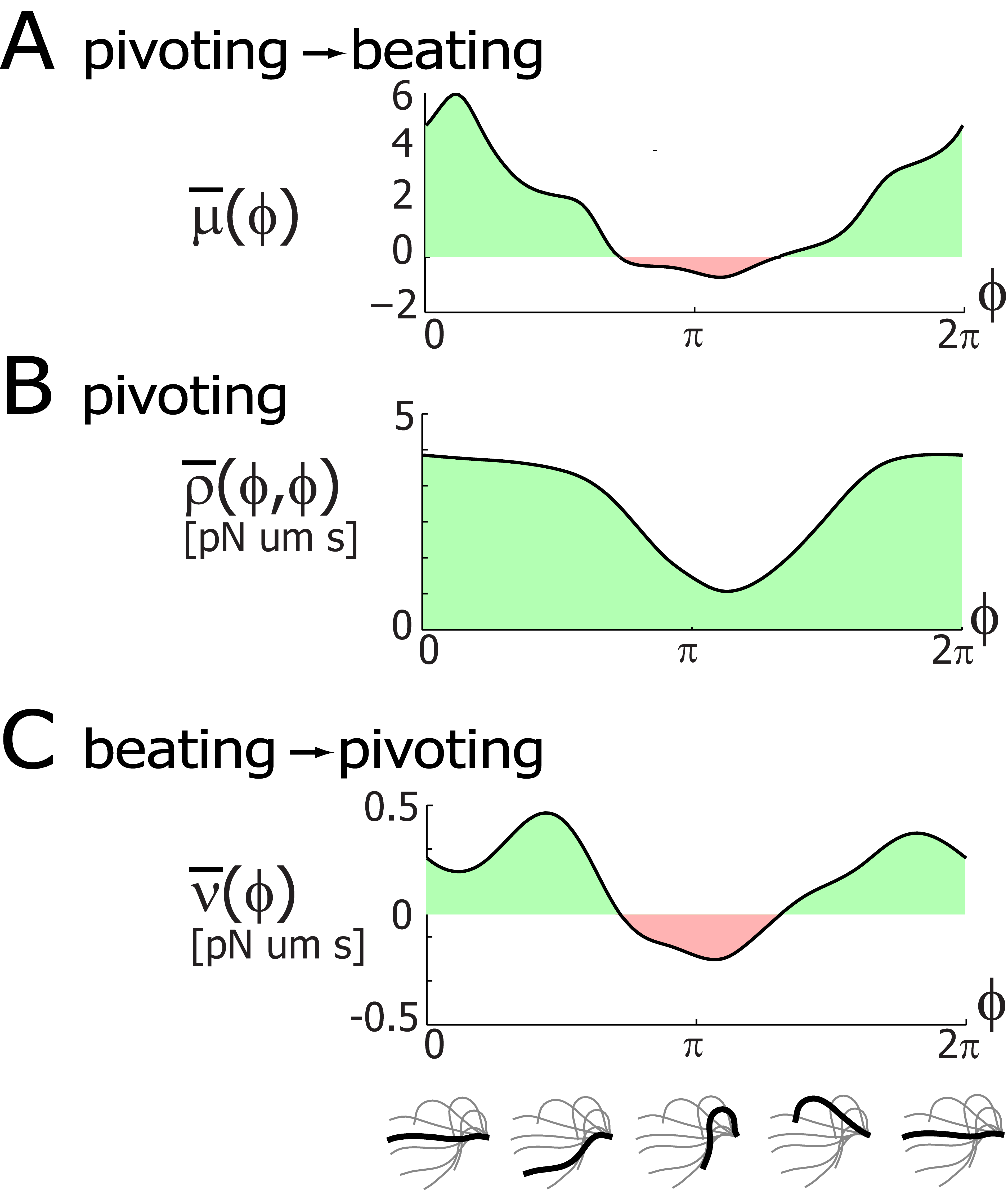
Figure S10: Theoretical coupling functions for the case of a pivoting flagellar base. A. A pivoting motion of the flagellar base changes the hydrodynamic friction force associated with flagellar beating and thereby speeds up or slows down the flagellar beat cycle in our theory. This effect is quantified by a coupling function $\overline{\mu}$, see equation S18. B. Hydrodynamic friction associated with pivoting of the flagellar base (and the attached flagella) is characterized by a friction coefficient $\overline{\rho}$, see equation S20. This friction coefficient is maximal when the two flagella extend maximally from the cell body during their effective stroke. C. The beat of the left flagellum causes pivoting of the flagellar base. This effect is quantified by a coupling function $\overline{\nu}$, see eqn. S20.

Here, the coupling functions $\overline{\mu}$, $\overline{\nu}$ and $\overline{\rho}$ play a similar role as the previously defined $\mu$, $\nu$ and $\rho$ for equation 2-4 and show a qualitatively similar dependence on the flagellar phase, see figure S10. To derive equations S18-S20, we neglected direct hydrodynamic interactions between the two flagella and approximated the active driving forces by $Q_{L}(\varphi)=\omega_{0}\Gamma_{LL}(\varphi,\varphi)_{|\psi=0}$ and $Q_{R}(\varphi)=\omega_{0}\Gamma_{RR}(\varphi,\varphi)_{|\psi=0}$. The coupling functions are defined as $\overline{\mu}(\varphi)=-\Gamma_{L\psi}(\varphi,\varphi)/\Gamma_{LL}(\varphi,\varphi)_{|\psi=0}$, $\overline{\nu}(\varphi)=-\Gamma_{\psi L}(\varphi,\varphi)_{|\psi=0}$, and $\overline{\rho}(\varphi,\varphi)=\Gamma_{\psi\psi}(\varphi_{L},\varphi_{R})_{|\psi=0}$. This choice retains the key nonlinearities of the full equation of motion, see also figure S3. Equation S18 states that pivoting of the flagellar basal apparatus with $\dot{\psi}>0$ slows down the effective stroke of the left flagellum (and speeds up the right flagellum). For synchronized flagellar beating, there will be no pivoting of the flagellar base. For asynchronous beating, however, the flagellar base will be rotated out of its symmetric rest position by an angle $\psi$ if the stiffness $\overline{k}$ is not too large. Any pivoting motion of the flagellar base during the beat cycle changes the hydrodynamic friction forces that oppose the flagellar beat, which in turn can either slow down or speed up the respective flagellar beat cycles, and thus restore flagellar synchrony.

To gain further analytical insight, we study the response of the dynamical system S18-S20 after a small perturbation $0<\delta(0)\ll 1$. To leading order in $\delta=\varphi_{L}-\varphi_{R}$, we find (with $\varphi\approx\omega_{0}t$)

$$\overline{k}\psi+\rho(\varphi,\varphi)\dot{\psi} =-d[\overline{\nu}(\varphi)\delta]/dt,$$ (S21)

$$\dot{\delta} =-2\overline{\mu}(\varphi)\dot{\psi},$$ (S22)

In the biologically relevant case of a relatively stiff basal anchorage of the flagellar basal apparatus with $\overline{k}\gg\rho\omega_{0}$, we find for the synchronization strength a result analogous to equation 6

$$\overline{\lambda}=-\oint_{0}^{2\pi}\!\!d\varphi\,\,\frac{\overline{\mu}(\varphi)\overline{\nu}^{\prime\prime}(\varphi)}{\overline{k}/\omega_{0}}.$$ (S23)

VII Supplementary Figures

Figure S1: Image analysis pipeline used to automatically track planar cell position and orientation as well as flagellar shapes in high-speed movies of swimming Chlamydomonas cells. 0. A typical movie frame 1. Rotated template images used for a cross-correlation analysis to estimate cell position and orientation in a movie frame. 2. The cell body outline was tracked by detecting intensity maxima (green) of line scans along rays (shown in blue), which emanate from the putative cell body center. From the cell body outline, we obtain refined estimates for cell position and orientation. 3. The position of the flagellar base was then determined using a fan of line-scans (along the blue lines), followed by a line-scan (green) in a direction perpendicular to the maximal intensity direction (red). 4. Finally, flagellar shapes were tracked in a successive manner using similar combinations of line-scans as in step 3.

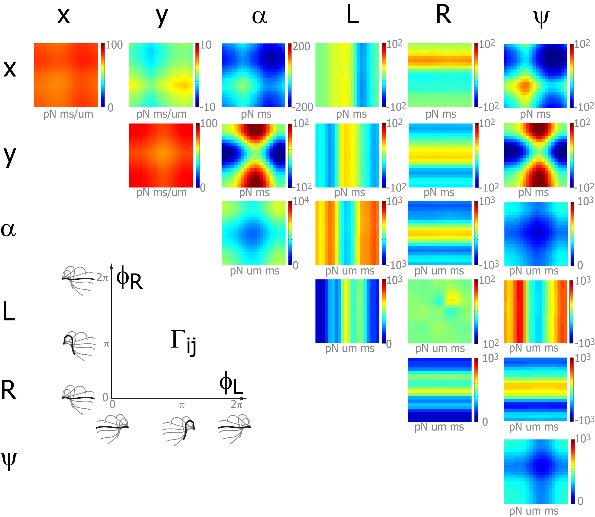
Figure S3: Generalized hydrodynamic friction matrix $\Gamma_{ij}$ associated with the effective degrees of freedom $x$, $y$, $\alpha$, $\varphi_{L}$, $\varphi_{R}$, $\psi$. This generalized friction matrix determines the generalized hydrodynamic friction forces $P_{i}$ conjugate to the degrees of freedom $\mathrm{q}=(x,y,\alpha,\varphi_{L},\varphi_{R},\psi)$ as $P_{i}=\Gamma_{ij}\dot{q}_{j}$, and is computed as a projection of the grand hydrodynamic friction matrix, see equation S7. Each friction coefficient $\Gamma_{ij}$ is a periodic function of the two phase angles $\varphi_{L}$ and $\varphi_{R}$, $\Gamma_{i,j}=\Gamma_{i,j}(\varphi_{L},\varphi_{R})$ and is represented as a colorplot with axes as indicated. Here, $\alpha$ is set to zero; different values of $\alpha$ would correspond to a simple rotation of the matrix shown. By Onsager symmetry, $\Gamma_{ij}=\Gamma_{ji}$ Landau:hydro . Several features are note-worthy: The coefficient $\Gamma_{LR}$ characterizes hydrodynamic interactions between the two flagella, and is found to be small compared to e.g. $\Gamma_{LL}$. The other coefficients $\Gamma_{Lj}=\Gamma_{jL}$, which set the friction force $P_{L}$ conjugate to $\varphi_{L}$, depend strongly on $\varphi_{L}$, but almost not on $\varphi_{R}$. This is yet another manifestation of the fact that direct hydrodynamic interactions between the two flagella are comparably weak. Analogous statements hold for the coefficients $\Gamma_{Rj}$. A counter-clockwise rotation of the cell, $\dot{\alpha}>0$, will increase the friction force $P_{L}$ during the effective stroke of the left flagellum ($\Gamma_{L\alpha}>0$), but decrease the corresponding the respective friction force $P_{R}$ for the right flagellum during its effective stroke ($\Gamma_{R\alpha}<0$). Mirror-symmetry of the swimmer amounts to invariance of the friction matrix under the substitution $(x,y,\alpha,\varphi_{L},\varphi_{R})\rightarrow(-x,y,-\alpha,\varphi_{R},\varphi_{L})$, which implies a number of symmetry relations, e.g. $\rho=\Gamma_{\alpha\alpha}$ must be symmetric in $\varphi_{L}$ and $\varphi_{R}$. Finally, this rotational friction coefficient $\rho=\Gamma_{\alpha\alpha}$ depends on the flagellar phases in a more pronounced way than the translational friction coefficients $\Gamma_{xx}$, $\Gamma_{yy}$. This is inline with the general fact that rotational friction coefficients depend stronger (as $\sim l^{3}$) on the effective linear dimension $l$ of an object than translational friction coefficients ($\sim l$). The coefficients $\Gamma_{j\alpha}$ and $\Gamma_{j\psi}$ associated with yawing of the whole cell and pivoting of the flagellar apparatus, respectively, show a similar dependence on the flagellar phases.

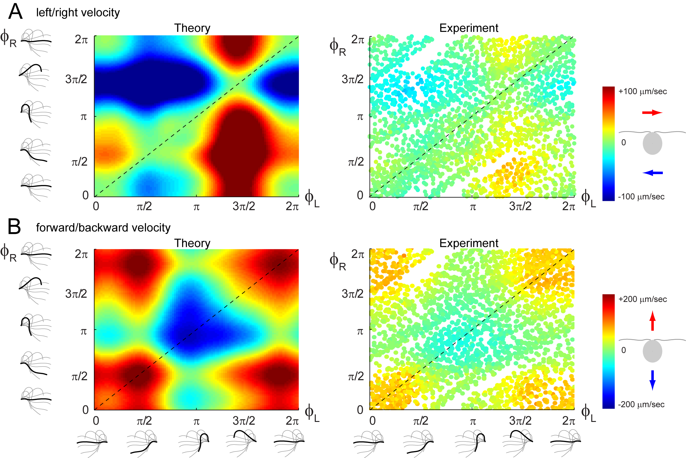
Figure S5: A. Instantaneous swimming velocity in the direction perpendicular to the long cell axis as a function of the flagellar phase angles $\varphi_{L}$ and $\varphi_{R}$. For synchronized flagellar beating (dashed line), this velocity vanishes in our theory for symmetry reasons (green). If the two flagella are out of synchrony, however, significant sidewards motion of the cell is observed, both in theory and experiment. Note that wall effects present in the experiments, but not considered in the computations, reduce translational velocities. B. Instantaneous swimming velocity in the direction of the long cell axis, again as a function of the flagellar phase angles.

Figure S6: The reduced equations of motion 2-4 were fitted to experimental time series data for the yawing rate $\dot{\alpha}$ of the cell, as well as the flagellar phase speeds $\dot{\varphi}_{L}$ and $\dot{\varphi}_{R}$. This provided experimental estimates for the phase-dependent coupling functions $\mu$, $\nu$, and $\rho$. Specifically, we represented each coupling function as a truncated Fourier series and determined the unknown Fourier coefficients by a linear regression using eqs. 2-4. A. Linear regression of equation 2. Shown to the left in black is the instantaneous flagellar phase speed of the left flagellum $\dot{\varphi}_{L}$ (smoothed with a span of $15\,\mathrm{ms}$). Shown in red is a reconstructed phase speed $\omega_{L}-\mu_{L}(\varphi_{L})\dot{\alpha}$ that depends on the instantaneous cell body yawing rate $\dot{\alpha}$, as well as the intrinsic flagellar frequency $\omega_{L}$ and phase-dependent coupling function $\mu_{L}$ for the left flagellum, which were obtained by the fit. The coefficient of determination was $R^{2}=30\%$. The estimate for $\mu_{L}$ obtained from this fit is shown to the right (blue), together with a theoretical prediction (black), see also figure 5A. B. Linear regression of equation 4. Shown to the left is the measured instantaneous yawing rate $\dot{\alpha}$ of the cell body (black), and a yawing rate reconstructed from the flagellar phase dynamics, $[-\nu(\varphi_{L})\dot{\varphi}_{L}+\nu(\varphi_{R})\dot{\varphi}_{R}]/\rho(\varphi_{L},\varphi_{R})$ (red). The coefficient of determination was $R^{2}=93\%$. From this fit, we obtain an experimental estimate for the coupling functions $\nu(\varphi)$ and $\rho(\varphi_{L},\varphi_{R})$ (blue); theoretical predictions are shown in black.

References

- (1) Alberts B, et al. (2002) Molecular Biology of the Cell (Garland Science, New York), 4th edition, p 1616.
- (2) Sanderson MJ, Sleigh MA (1981) Ciliary activity of cultured rabbit tracheal epithelium: beat pattern and metachrony. J. Cell Sci. 47:331–47.
- (3) Gray J (1928) Ciliary Movements (Cambridge Univ. Press, Cambridge).
- (4) Osterman N, Vilfan A (2011) Finding the ciliary beating pattern with optimal efficiency. Proc. Natl. Acad. Sci. U.S.A. 108:15727–32.
- (5) Brennen C, Winet H (1977) Fluid mechanics of propulsion by cilia and flagella. Ann. Rev. Fluid Mech. 9:339–398.
- (6) Pikovsky A, Rosenblum M, Kurths J (2001) Synchronization (Cambridge UP).
- (7) Taylor GI (1951) Analysis of the swimming of microscopic organisms. Proc. Roy. Soc. Lond. A 209.:447–461.
- (8) Gueron S, Levit-Gurevich K (1999) Energetic considerations of ciliary beating and the advantage of metachronal coordination. Proc. Natl. Acad. Sci. U.S.A. 96:12240–5.
- (9) Vilfan A, Jülicher F (2006) Hydrodynamic flow patterns and synchronization of beating cilia. Phys. Rev. Lett. 96:58102.
- (10) Niedermayer T, Eckhardt B, Lenz P (2008) Synchronization, phase locking, and metachronal wave formation in ciliary chains. Chaos 18:037128.
- (11) Golestanian R, Yeomans JM, Uchida N (2011) Hydrodynamic synchronization at low Reynolds number. Soft Matter 7:3074.
- (12) Friedrich BM, Jülicher F (2012) Flagellar synchronization independent of hydrodynamic interactions. Phys. Rev. Lett. 109:138102.
- (13) Bennett RR, Golestanian R (2013) Emergent Run-and-Tumble Behavior in a Simple Model of Chlamydomonas with Intrinsic Noise. Phys. Rev. Lett. 110:148102.
- (14) Polotzek K, Friedrich BM (2013) A three-sphere swimmer for flagellar synchronization. New J. Phys. 15:045005.
- (15) Rüffer U, Nultsch W (1985) High-speed cinematographic analysis of the movement of Chlamydomonas. Cell Mot. 5:251–263.
- (16) Rüffer U, Nultsch W (1998) Flagellar coordination in Chlamydomonas cells held on micropipettes. Cell Motil. Cytoskel. 41:297–307.
- (17) Polin M, Tuval I, Drescher K, Gollub JP, Goldstein RE (2009) Chlamydomonas swims with two “gears” in a eukaryotic version of run-and-yumble. Science 325:487–490.
- (18) Goldstein RE, Polin M, Tuval I (2009) Noise and synchronization in pairs of beating eukaryotic flagella. Phys. Rev. Lett. 103:168103.
- (19) Tam D, Hosoi AE (2011) Optimal feeding and swimming gaits of biflagellated organisms. Proc. Natl. Acad. Sci. U.S.A. 108:1001–6.
- (20) Bayly PV, et al. (2011) Propulsive forces on the flagellum during locomotion of Chlamydomonas reinhardtii. Biophys. J. 100:2716–25.
- (21) O’Malley S, Bees MA (2012) The orientation of swimming biflagellates in shear flows. Bull. Math. Biol. 74:232–55.
- (22) Brokaw CJ (1975) Effects of viscosity and ATP concentration on the movement of reactivated sea-urchin sperm flagella. J. exp. Biol. 62:701–19.
- (23) Garcia M, Berti S, Peyla P, Rafaï S (2011) Random walk of a swimmer in a low-Reynolds-number medium. Physical Review E 83:1–4.
- (24) Hunt AJ, Gittes F, Howard J (1994) The force exerted by a single kinesin molecule against a viscous load. Biophys. J. 67:766–781.
- (25) Happel J, Brenner H (1965) Low Reynolds Number Hydrodynamics (Kluwer, Boston, MA).
- (26) K. Hinsen (1995) HYDR0LIB : a library for the evaluation of hydrodynamic interactions in colloidal suspensions. Comp. Phys. Comm. 88:327–340.
- (27) Racey TJ, Hallett R, Nickel B (1981) A quasi-elastic light scattering and cinematographic investigation of motile Chlamydomonas reinhardtii. Biophysical journal 35:557–71.
- (28) Guasto J, Johnson K, Gollub J (2010) Oscillatory flows induced by microorganisms swimming in two dimensions. Phys. Rev. Lett. 105:18–21.
- (29) Reichert M, Stark H (2005) Synchronization of rotating helices by hydrodynamic interactions. Eur. Phys. J. E 17:493–500.
- (30) Hyams JS, Borisy GG (1975) Flagellar coordination in Chlamydomonas reinhardtii: isolation and reactivation of the flagellar apparatus. Science 189:891–3.
-
(31)
Gorman D, Levine R
(1965) Cytochrome f and plastocyanin: their sequence in the
photosynthetic electron transport chain of Chlamydomonas reinhardii.
Proc. Natl. Acad. Sci. U.S.A. 54:1665–1669.
Supporting Information References
- (32) Riedel-Kruse IH, Hilfinger A, Howard J, Jülicher F (2007) How molecular motors shape the flagellar beat. HFSP J. 1:192–208.
- (33) Friedrich BM, Riedel-Kruse IH, Howard J, Jülicher F (2010) High-precision tracking of sperm swimming fine structure provides strong test of resistive force theory. J. exp. Biol. 213:1226–1234.
- (34) Scholkopf B, Smola AJ, Bernhard S (2002) Learning with Kernels: Support Vector Machines, Regularization, Optimization, and Beyond (Adaptive Computation and Machine Learning) (MIT Press, Cambridge, USA), p 648.
- (35) Perrin F (1934) Mouvement Brownien d’un ellipsoide (I). Dispersion dièlectrique pour des molécules ellipsoidales. Le Journal de Physique et le Radium 7:497–511.
- (36) Gray J, Hancock GT (1955) The propulsion of sea-urchin spermatozoa. J. exp. Biol. 32:802–814.
- (37) Goldstein H, Poole C, Safko J (2002) Classical Mechanics (Addison-Wesley, Reading, MA), 3rd edition, p 680.
- (38) Ringo DL (1967) Flagellar motion and the fine structure of the flagellar apparatus in Chlamydomonas. Cell 33:543–571.
- (39) Landau LD, Lifshitz EM (1987) Fluid Mechanics (Butterworth-Heinemann, New York).