Realistic Simulations of Stellar Surface Convection with ANTARES:
I. Boundary Conditions and Model Relaxation

Abstract

We have implemented open boundary conditions into the ANTARES code to increase the realism of our simulations of stellar surface convection. Even though we greatly benefit from the high accuracy of our fifth order numerical scheme (WENO5), the broader stencils needed for the numerical scheme complicate the implementation of boundary conditions. We show that the effective temperature of a numerical simulation cannot be changed by corrections at the lower boundary since the thermal stratification does only change on the Kelvin–Helmholtz time scale. Except for very shallow models, this time scale cannot be covered by multidimensional simulations due to the enormous computational requirements. We demonstrate to what extent numerical simulations of stellar surface convection are sensitive to the initial conditions and the boundary conditions. An ill-conceived choice of parameters for the boundary conditions can have a severe impact. Numerical simulations of stellar surface convection will only be (physically) meaningful and realistic if the initial model, the extent and position of the simulation box, and the parameters from the boundary conditions are chosen adequately.

1 Introduction

Nowadays, realistic simulations of stellar surface convection are a mature tool of computational astrophysics, and find a wide field of applications. An extensive review on this subject is given in Nordlund et al. (2009). Beeck et al. (2012) illustrate the usefulness and reliability of results obtained from simulations of solar surface convection with the codes CO5BOLD, MURaM and Stagger. Despite the differences in numerical schemes and atomic physics between the simulations they compared, the overall stratification and other basic properties of the numerical models are similar.

For any numerical simulation which requires the solution of partial differential equations, the choice of the numerical method, the simulation domain, and appropriate boundary conditions are of major importance. For the simulation of convection at the surface of solar-type stars, the top boundary of the simulation domain is in the upper photosphere, and the bottom boundary is situated inside the convective envelope. The bottom boundary conditions determine the adiabat of the deep convection zone (the part interior to the simulation), and therefore the effective temperature $T_{\rm eff}$ of the simulation.

The ANTARES code was originally developed at the University of Vienna for the simulation of surface convection (Muthsam et al., 2007, 2010a; Lemmerer et al., 2013). Recently, the code was also applied to many other astrophysical problems (Kupka et al., 2009; Muthsam et al., 2010b; Kupka et al., 2012; Happenhofer et al., 2013; Zaussinger and Spruit, 2013; Mundprecht et al., 2013). In some of these applications problems arose due to the use of closed boundary conditions (Kupka et al., 2009; Mundprecht et al., 2013). Shock fronts were reflected at the top boundary, leading to numerical instabilities.

Robinson et al. (2003), Kupka and Robinson (2007) and Kupka (2009a, b) discussed, amongst others, the effect of boundary conditions on statistical properties of the flow. Unrealistic boundary conditions can lead to unphysical flow patterns in most of the simulation box. When the bottom boundary is situated in the convective region of the star, which usually is the case, e.g., for solar surface convection simulations, a vast majority of the energy is transported in the lower part of the simulation box by advection of enthalpy (the convective flux) and kinetic energy. Therefore, the boundary conditions should allow transport of energy by convective motions avoiding the need of feeding in the energy by an artificial radiative source term. At the bottom boundary, the entropy of the inflowing material is unknown and has to be specified somehow. At the top boundary, shock fronts should not be reflected, but be transmitted.

Even though a lot of literature exists on stellar surface convection simulations (e.g., Nordlund, 1982; Freytag et al., 2012; Vögler et al., 2005; Jacoutot et al., 2008), a thorough investigation of the boundary conditions effects on the simulations appears to be missing. This paper gives a detailed description of the numerical schemes of our surface convection simulations with ANTARES and investigates the sensitivity of the simulations to changes in the boundary conditions.

A two-dimensional geometry leads to systematic differences in the mean stratification such that, for instance, a different inflow entropy is required to obtain the same total flux at the stellar surface (Asplund et al., 2000). Meaningful tests of boundary conditions can ultimately only be done in three dimensions, with sufficient resolution and long relaxation time. Despite the nearly linear scaling of our code (Happenhofer et al., 2013), this makes this investigation very expensive in terms of computation time as well as in wall-clock time.

The results of the present paper provide a necessary extension to comparisons shown in Kupka (2009a) and Beeck et al. (2012), where simulations produced with independent codes were compared. Performing a systematic parameter-space exploration of our boundary conditions is simply not affordable. Instead we restrict ourselves to the most relevant and fruitful regions of parameter-space. In this paper, we show results from several working and non-working combinations and estimate the impact of inappropriately designed boundary conditions.

The remainder of the paper is organised as follows. In Section 2.1, we describe the details of our implementation of several boundary conditions inspired by those used in the CO5BOLD–, MURaM– and Stagger–codes. The numerical setup of our simulations, i.e. the starting model and the simulation box size, is described thoroughly in Section 2.2.

We then investigate the effect of using different boundary conditions and compare them, taking statistical properties of the flow into account, in Sections 3.1 and 3.2. We show the difficulties arising in the setup of the simulation, its dependence on the initial model (Section 3.3) and on the grid resolution (Section 3.4), and emphasize the importance of a careful choice of parameters. In Section 3.5, we describe differences between simulations with open and with closed boundary conditions. Finally, we compare two- and three-dimensional models in Section 3.6. A discussion of the results can be found in Section 4 followed by our conclusions in Section 5. Finally, in A we describe how oscillations can be damped, in B how boundary conditions on the gradient are implemented, and in C how energy fluxes are calculated.

2 Boundary Conditions and Initial Models

In this section, we describe the implementation of several boundary conditions in the code ANTARES as well as other modifications to the code we have performed in this context.

In this document, the ANTARES convention for spatial coordinates is used. The ANTARES code uses a right-handed coordinate system with the $x$–axis pointing into the star. $u$ is the vertical component of the velocity vector $(u,v,w)^{T}$. The grid is equidistant in every direction. The methods presented in the following section, however, are not limited to an equidistant grid.

The equations we solve are the Navier–Stokes equations

$$\frac{\partial\rho}{\partial t}+\nabla\cdot\left(\rho{\bf u}\right) =0,$$ (1a)

$$\frac{\partial\left(\rho{\bf u}\right)}{\partial t}+\nabla\cdot\left(\rho{\bf u}{\bf u}\right)+\nabla p =\rho{\bf g}+\nabla\cdot\tau,$$ (1b)

$$\frac{\partial E}{\partial t}+\nabla\cdot\left({\bf u}\left(E+p\right)\right) =\rho\left({\bf g}\cdot{\bf u}\right)+\nabla\cdot\left({\bf u}\cdot\tau\right)+Q_{\rm rad},$$ (1c)

where ${\bf g}$ is the gravity vector and $Q_{\rm rad}$ is the radiative heating rate describing the energy exchange between gas and radiation (cf. Muthsam et al. 2010a). The viscous stress tensor $\tau=\left(\tau_{i,j}\right)_{i,j=1,2,3}$ is given by

$$\tau_{i,j}=\eta\left(\frac{\partial u_{i}}{\partial x_{j}}+\frac{\partial u_{j}}{\partial x_{i}}-\frac{2}{3}\delta_{i,j}\left(\nabla\cdot{\bf u}\right)\right)+\zeta\,\delta_{i,j}\left(\nabla\cdot{\bf u}\right).$$ (2)

$\delta_{i,j}$ is the Kronecker symbol. $\eta$ and $\zeta$ are the first and second coefficients of viscosity. We use the LLNL equation of state from Rogers et al. (1996), the OPAL opacities from Iglesias and Rogers (1996) and the composition from Grevesse and Noels (1993). Our standard initial model is model S from Christensen-Dalsgaard et al. (1996) which is calibrated to match helioseismic inversions and uses the same equation of state, opacities, and chemical composition.

For the spatial discretisation of the advective part of the Navier–Stokes equations, ANTARES uses the weighted essentially non-oscillatory (WENO) algorithm as described, e.g., in Jiang and Shu (1996) and Shu (2003). WENO schemes exist for any order of accuracy. In ANTARES, we use the fifth order variant which will be called WENO5 in the following (Muthsam et al., 2010a), without any artificial stabilisation terms. The advantages of the WENO5 method are its high order of accuracy in smooth flow regions and its shock-capturing ability. This allows accurate modelling of surface convection where strong shock fronts are ubiquitous in the photosphere, whereas the granules themselves are rather smooth (cf. Nordlund et al. 2009). The appropriate treatment of diffusive and viscous terms in the context of WENO5 is discussed in detail in Happenhofer et al. (2013).

The high accuracy of a fifth-order scheme, combined with the stability of WENO into the WENO5 algorithm used in ANTARES as shown in Muthsam et al. (2007) and Muthsam et al. (2010a) justifies the use of broader stencils needed for any high-order method. In the design of the boundary conditions, we must keep in mind that the boundary extends over several vertical layers.

2.1 Boundary Conditions for Stellar Convection Simulations

For solar-like main-sequence stars, the characteristic scale of surface convection is small compared to the stellar radius and, hence, the “box–in–a–star” approximation is valid for the simulation of surface convection. When the turbulent kinetic energy of the simulation is unaffected by a further increase in aspect ratio of the domain, periodic boundary conditions can be used at the horizontal boundaries (Robinson et al., 2003).

In the vertical direction, the top boundary is typically placed above the photosphere whereas the bottom boundary is in the upper part of the convective envelope (Stein and Nordlund, 1998; Robinson et al., 2003; Wedemeyer-Böhm et al., 2004; Freytag et al., 2012; Vögler et al., 2005; Muthsam et al., 2007, 2010a). Numerical boundary conditions either force the fluid to stop its vertical motion (the so called closed boundary conditions) and hence not cross the vertical boundary, or they allow in-­ and outflow (open boundary conditions). In each of these two classes, there are many variants available for the design of specific boundary conditions.

Simulations from Stein et al. (2009) show that the dominant horizontal scale of the convection increases monotonically with increasing depth in the uppermost $\sim 20\,{\rm Mm}$ of the solar convection zone, whereas the area ratio of upflows to downflows is nearly independent of depth, and the average energy fluxes stay nearly constant. There is no physical reason why the vertical convective motions should stop at the boundary of the simulation domain situated significantly above the boundary of their simulations as it is forced by closed boundary conditions. To increase the physical realism of the simulation it is mandatory to allow free in- and outflow at the boundaries. But the design of stable and benign open boundary conditions is non-trivial, as we show in the following. Since we intend to use symmetric stencils at the boundary, the boundary conditions must be set on several layers corresponding to the width of the stencils.

2.1.1 Closed Boundaries

Slip (stress-free) boundary conditions are characterised by setting the vertical velocity component and the vertical derivative of the horizontal velocities to $0$, i.e.

$$u=0,\ \frac{\partial v}{\partial x}=\frac{\partial w}{\partial x}=0.$$ (3a)

Furthermore, since the bottom boundary can transport energy only by radiation, an artificial source term must be introduced to feed the required amount of energy into the simulation domain. This is done by modifying the thermal conductivity $k$ in the lowermost layers of the simulation domain such that

$$-k_{{\rm modified}}\frac{\partial T}{\partial x}=F_{\star}=\sigma T_{\rm eff}^{4},$$ (3b)

and imposing $\frac{\partial\rho}{\partial x}=0$. The detailed scheme is described, e.g., in Robinson et al. (2003) and Muthsam et al. (2010a).

Closed boundary conditions have the advantage of simplicity and high stability, at least for subsonic flows. On the other hand, they reflect shocks and disturb the velocity field in undesirable ways, as discussed by Robinson et al. (2003), Kupka et al. (2009), and Kupka (2009a). Effects on the thermodynamics are indirect at most, e.g. through the reflection of shocks. Nevertheless, there are applications where the use of closed boundary conditions is not problematic, such as the numerical simulation of the superadiabatic layer (SAL in the following) of the Sun (Kim and Chan, 1998; Robinson et al., 2003; Kupka and Robinson, 2007; Kupka, 2009a; Tanner et al., 2012, 2013). Moreover, for hotter main-sequence stars, e.g., the surface convection zone is shallow such that the whole convection zone can be contained in the simulation domain, and the lower boundary is in the underlying radiative zone. On the other hand, the top boundary should be open in their case, too, due to the ubiquity of shocks.

2.1.2 Open Top Boundary Conditions

The top boundary of simulations of surface convection typically is located in the photosphere, i.e. the region where the optical Rosseland depth $\tau$ is between $10^{-6}$ and $10$. We implemented the top boundary conditions presented in Cheung (2006) and Trampedach (1997) with some slight modifications which will be described in the following. Generally speaking, the boundary conditions should be designed in such a way that they do not influence the behaviour of the flow. For the top boundary layers, we assume a hydrostatic and isoenergetic stratification. For the Sun and the LLNL equation of state, this implies nearly isothermal stratification. As a difference to previous implementations, in the hydrostatic equilibrium we want to include the turbulent pressure since it amounts to $\sim 10\,\%$ of the total mean pressure in the photosphere, which is of similar magnitude as in the SAL (the maximum of $\sim 15\,\%$ is reached around $100\,{\rm km}$ below the stellar surface). The velocities are constantly extrapolated according to

$$\frac{\partial u}{\partial x}=\frac{\partial v}{\partial x}=\frac{\partial w}{\partial x}=0$$ (4a)

to make the boundary transmissive for waves. In order to use the symmetric stencils of the fifth order WENO method at the boundary, the boundary conditions must extend over three fiducial layers.

We assign the indices $-2$, $-1$ and $0$ to the fiducial layers and number the domain layers starting with $1$ at the top of the domain. The mean density in layer $0$, $\langle\rho\rangle_{0}$, is advanced in time by the continuity equation (1a) setting the mean mass flux from the top to $0$, i.e.

$$\langle\rho\rangle_{0}^{(n+1)}=\langle\rho\rangle_{0}^{(n)}-\frac{{\Delta t}_{\rm stg}}{\Delta x}\langle\rho u\rangle_{\frac{1}{2}}^{(n)},$$ (4b)

where ${\Delta t}_{\rm stg}$ is the time step size of the current Runge–Kutta stage and $\Delta x$ is the (constant) vertical grid spacing. $n$ is the number of the current time step. $\langle\rho u\rangle_{\frac{1}{2}}^{(n)}$, the mean density flux at the mid-point between the layers $0$ and $1$, can be computed using the standard symmetric stencils. With the mean density in layer $0$ obtained using (4b), the density profile layer in $0$ is just copied from layer $1$ scaled by the ratio $\frac{\langle\rho\rangle_{0}^{(n+1)}}{\langle\rho\rangle_{1}^{(n+1)}}$, i.e.

$$\rho_{0}^{(n+1)}(y,z)=\frac{\langle\rho\rangle_{0}^{(n+1)}}{\langle\rho\rangle_{1}^{(n+1)}}\rho_{1}^{(n+1)}(y,z).$$ (4c)

The specific internal energy $\langle\epsilon\rangle_{0}$ in all boundary layers is assumed to be constant in space. It is initialised by the mean specific internal energy in the outermost domain layer $\langle\epsilon\rangle_{1}$ and is furthermore advanced in time by

$$\langle\epsilon\rangle_{0}^{(n+1)}=(1.0-\delta)\langle\epsilon\rangle_{0}^{(n)}+\delta\langle\epsilon\rangle_{1}^{(n+1)}.$$ (4d)

Cheung (2006) set $\delta$ constantly to $10^{-3}$, but we reset $\langle\epsilon\rangle_{0}$ only at the end of each Runge–Kutta step with $\delta$ given by the formula

$$\delta=\frac{\Delta t\cdot\langle v_{\rm snd}\rangle_{1}}{c_{\rm f}\cdot\langle H\rangle_{1}},$$ (4e)

where $\Delta t$ is the time step of one Runge-Kutta integration, $\langle v_{\rm snd}\rangle_{1}$ is the mean sound speed in layer $1$ and $\langle H\rangle_{1}$ the mean pressure scale height in that layer. With the parameter $c_{\rm f}$ we can control $\delta\in[0,1]$, i.e. the time scale on which the heat content of the boundary layers varies. Higher values of $c_{\rm f}$ lead to slower changes. By using $\langle H\rangle_{1}$ instead of the geometrical height of the computational cell, we keep $\delta$ unchanged when the vertical resolution of the simulation is changed. Since $c_{\rm f}$ has to be adjusted anyway, it is sufficient to use the gas pressure to compute $\langle H\rangle_{1}$ for the approximate time scale underlying (4e).

The idea behind equation (4e) is to make the procedure independent of different time integration methods and spatial resolution. With a constant value of $\delta$, the time scale of changing $\langle\epsilon\rangle_{0}$ would be different, if a two- or a three-stage Runge–Kutta method is used, or if the Courant number is changed. Furthermore, we choose $\delta$ independent of the grid spacing such that the time scale does not change if the grid is modified. Modifying $c_{\rm f}$ allows to control the stability and the stratification of the boundary layers.

The density in the layers above index $0$ is assumed to be pointwisely in hydrostatic equilibrium

$$\frac{\partial(p+p_{\rm turb})}{\partial x}=-\rho g,$$ (4f)

where $p=p_{\rm rad}+p_{\rm gas}$ and $p_{\rm turb}=\rho\left(u-\langle u\rangle\right)^{2}$ is the turbulent pressure. By the chain rule and due to equation (4a),

$$\frac{\partial(p+p_{\rm turb})}{\partial x}=\frac{\partial\left(p+p_{\rm turb}\right)}{\partial\rho}\frac{\partial\rho}{\partial x}=\left(\frac{\partial p}{\partial\rho}+\left(u-\langle u\rangle\right)^{2}\right)\frac{\partial\rho}{\partial x}.$$ (4g)

For a perfect gas, constant $\epsilon$ implies an isothermal stratification. The slight deviations of $T$, evaluated from the LLNL equation of state, from its horizontal mean therefore show the deviation from the perfect gas equation. Since in our simulations, these deviations rarely exceed $5\,\%$, it is reasonable to assume the simplification of a perfect gas in the boundary layers, considering the other simplifications like constant velocity and constant $\epsilon$. In this case, $\frac{\partial p}{\partial\rho}=\left(\gamma-1\right)\epsilon$ is constant in the boundary layer.

Since $\left(u-\langle u\rangle\right)^{2}$ in the boundary layer is constant in the vertical direction due to (4a), the value $c_{\rho}:=\frac{\partial p}{\partial\rho}+\left(u-\langle u\rangle\right)^{2}$ is constant vertically, but varies horizontally. Therefore, we can integrate equation (4g) analytically and obtain

$$\rho(i,y,z)=\rho(0,y,z)\exp\left(\frac{-|i|\Delta x\cdot g}{c_{\rho}}\right),$$ (4h)

where $i=-1,-2$. With $\langle\epsilon\rangle_{0}$ and the velocities calculated by (4a), all values in all boundary layers can be calculated.

2.1.3 Open Bottom Boundary Conditions

We formulate two sets of boundary conditions, the first one based on Nordlund and Stein (1990) and Freytag et al. (2012), and the second one on Vögler et al. (2005).

Nordlund and Stein (1990) and Freytag et al. (2012) set density and internal energy such that the inflows have a certain entropy value. This entropy value is fixed in space and time and found by trial and error or by using previous simulations (see Fig. 3 in Ludwig et al. 1999 and Fig. 1 in Trampedach et al. 2013). Finally, the velocities in the outflows are scaled to obtain an average mass flux of $0$ at the lower boundary.

Instead of prescribing an entropy value, Vögler et al. (2005) chose to set the specific internal energy of an inflow through a feed-back loop. Since in a relaxed simulation, the radiative flux at the top of the domain corresponds to the amount of energy flowing through the bottom boundary, Vögler et al. (2005) decided to directly correlate the two values on the Kelvin–Helmholtz time scale. When the radiative flux at the top is too high, the amount of energy flowing in at the bottom is lowered which in principle leads to a lower radiative flux. This motivated the formula

$$\epsilon_{\rm inflow}^{(n+1)}=\epsilon_{\rm inflow}^{(n)}\cdot\left[1.0+\frac{\Delta t}{\tau_{\rm KH}}\left(1.0-\frac{F_{\rm rad}^{\rm top}}{F_{\star}}\right)\right],$$ (5)

where $F_{\star}=\sigma T_{\rm eff}^{4}$ is the energy flux of the star according to the Stefan–Boltzmann law and $\Delta t$ the time step size of one Runge–Kutta integration. The Kelvin–Helmholtz time scale $\tau_{\rm KH}$ can be calculated as

$$\tau_{\rm KH}=\frac{\int_{{\rm box}}\rho\epsilon\,dV}{\int_{\rm top}F_{\rm rad}\,dy\,dz}$$ (6)

(cf. formula (19) and (20) in Vögler et al. 2005). They correct the density at the lower boundary to keep the total mass in the simulation domain unaltered. The entropy of an inflow will vary with the changing density.

We implemented both approaches which define either $S_{\rm inflow}$ or $\epsilon_{\rm inflow}$ into our code and show results in Section 3.2. In those cases where we specify $S_{\rm inflow}$ at the bottom, we use an iterative correction procedure similar to (5), which is used for $\epsilon_{\rm inflow}$. In the first variant, we only change the time scale and define

$$S_{\rm inflow}^{(n+1)}=S_{\rm inflow}^{(n)}\cdot\left[1.0+\frac{\Delta t}{\tau_{\rm S}}\left(1.0-\frac{F_{\rm rad}^{\rm top}}{F_{\star}}\right)\right],$$ (7)

where $\tau_{\rm S}$ is the time scale of the correction. In general, $\tau_{\rm S}\neq\tau_{\rm KH}$ since we expect much smaller changes in $S$ than in $\epsilon$. In the limits $\tau_{\rm S}\to\infty$ and $F_{\rm rad}^{\rm top}\to F_{\star}$, $S_{\rm inflow}={\rm constant}$ as in Nordlund and Stein (1990) and Freytag et al. (2012).

In the second variant, it is guaranteed that the total flux at the bottom boundary is close to $F_{\star}$. Here,

$$S_{\rm inflow}^{(n+1)}=S_{\rm inflow}^{(n)}\cdot\left[1.0+\frac{\Delta t}{\tau_{\rm S}}\left(1.0-\frac{F_{\rm tot}^{\rm bot}}{F_{\star}}\right)\right],$$ (8)

where $F_{\rm tot}^{\rm bot}$ is the sum of the radiative, the kinetic, and the convective fluxes at the bottom of the domain. In this case, $\tau_{\rm S}$ must be set according to the time scale on which $F_{\rm tot}^{\rm bot}$ changes to avoid decoupling of the correction mechanism from the correction quantity.

None of these correction mechanisms should be applied during transients excited by any changes such as scaling of variables of the simulation. Both the radiative flux at the top and the total flux at the bottom require some time to reach the value which reflects the current thermal stratification. Therefore, we do not change $S_{\rm inflow}$ during the first five sound crossing times of a new model started from a one-dimensional stratification.

In the following, we describe our implementation of the boundary conditions following Freytag et al. (2012) in detail. We assume the velocities to be constant with depth

$$\frac{\partial u}{\partial x}=\frac{\partial v}{\partial x}=\frac{\partial w}{\partial x}=0.$$ (9)

Then, we calculate the density $\rho$ and the specific internal energy $\epsilon$ in the boundary layers. Superscript numbers in paranthesis denote different correction levels. In the first correction step of Freytag et al. (2012), $\rho$ and $\epsilon$ are reset by

$$\rho^{(1)} =\rho+\delta_{S}\frac{\Delta t}{t_{\rm char}}\frac{-\rho^{2}T(\Gamma_{3}-1)}{p\Gamma_{1}}\left(S_{\rm inflow}-S\right),$$ (10a)

$$\epsilon^{(1)} =\epsilon+\delta_{S}\frac{\Delta t}{t_{\rm char}}T\left(1-\frac{\Gamma_{3}-1}{\Gamma_{1}}\right)\left(S_{\rm inflow}-S\right),$$ (10b)

(cf. (34) and (35) from Freytag et al. 2012) with the parameter $\delta_{S}$ controlling the time scale of the correction step. $\Delta t$ is the time step size of the (Runge–Kutta) integration and the characteristic time-scale for the adjustments is given by

$$t_{\rm char}=\frac{\Delta x}{\langle v_{\rm snd}+\left|u\right|\rangle}$$ (10c)

(cf. (33) from Freytag et al. 2012). The adiabatic sound speed $v_{\rm snd}$ as well as the adiabatic coefficients $\Gamma_{1}$ and $\Gamma_{3}$ are evaluated from the equation of state as a function of the uncorrected values of $\rho$ and $\epsilon$.

In our implementation, however, we obtain $\epsilon^{(1)}$ and $\rho^{(1)}$ from performing an isobaric entropy change, i.e. we invert the equation of state such that

$$S(\rho^{(1)},\epsilon^{(1)})=S_{\rm inflow}^{(n+1)},$$ (11)

without changing $p$. $S_{\rm inflow}^{(n+1)}$ is determined either with (7) or (8). Entropy, internal energy, and density of an outflow are not changed. In this way, we delete the parameter $\delta_{S}$ from the formulation of the boundary conditions.

We then proceed with two additional correction steps proposed by Freytag et al. (2012) which avoid the generation of unwanted large pressure fluctuations by the inflow at the open bottom boundary, and fix the mean mass flux over the boundary to $0$. Thus, as in the second correction step from Freytag et al. (2012), density and specific internal energy throughout the entire boundary layers are reset by

$$\rho^{(2)} =\rho^{(1)}+\delta_{p}\frac{\Delta t}{t_{\rm char}}\frac{1}{v_{\rm snd}^{2}}\left(\langle p\rangle-\,p\right),$$ (12a)

$$\epsilon^{(2)} =\epsilon^{(1)}+\delta_{p}\frac{\Delta t}{t_{\rm char}}\frac{1}{\Gamma_{1}\rho}\left(\langle p\rangle-\,p\right)$$ (12b)

(cf. (36) and (37) from Freytag et al. 2012). The parameter $\delta_{p}$ governs the time scale on which pressure fluctuations are reduced.

Finally, $\rho$ and the vertical velocity $u$ are modified by

$$\rho^{(3)} =\rho^{(2)}+\langle\rho\rangle^{(0)}-\langle\rho^{(2)}\rangle,$$ (12c)

$$u^{(1)} =u-\frac{\langle\rho^{(3)}u\rangle}{\langle\rho\rangle^{(0)}}$$ (12d)

(cf. (38) and (39) from Freytag et al. 2012) to keep the total mass at the bottom boundary unaltered. Again, this correction is applied throughout the entire boundary layers.

As for the top boundary at the bottom three boundary layers are needed for the WENO scheme used in ANTARES. After the procedure described above is applied to the innermost boundary layer at the bottom, the two underlying layers are filled by exponentially extrapolating the density and by linearly extrapolating the specific internal energy (assuming adiabatic stratification instead would require to proceed as in Sect. 2.2.2 to recover the power law growth with depth, possibly with a correction for turbulent pressure as in (4f) and (4g), but we expect the difference to our simplified procedure along the two outer grid points to be acceptably small).

When implementing the boundary conditions which are similar to Freytag et al. (2012), care must be taken in the formulation of mass conservation. Instead of the variable $\rho u$, the numerical density flux situated at the half-integer node must be set to $0$. The system is not overdetermined when we enforce this condition, since it is only another numerical consequence of the (analytical) mass conservation requirement.

Furthermore, as another available alternative to the open bottom boundary conditions specified by (7) or (8), (9), (11), and (2.1.3), we implemented the full version of boundary conditions from Vögler et al. (2005) into our code. For the present paper these are used only for the case of Model 2 in Section 3.2. In these boundary conditions, in addition to specifying the inflow internal energy by (5), the pressure is assumed to be uniform across the lower boundary. Its value $p_{\rm tot}$ is determined to keep the mass in the simulation box unaltered (see equations (21) to (23) in the cited reference).In inflow regions, Vögler et al. (2005) force the inflow to be vertical (cf. (18) therein). In contrast, the velocities are set by (9) in our implementation. In downflow regions, the velocities and the entropy density $S$ are set according to

$$\frac{\partial u}{\partial x}=\frac{\partial v}{\partial x}=\frac{\partial w}{\partial x}=0,\,\frac{\partial S}{\partial x}=0,$$ (13)

(see equations (16) and (17) in the same reference).

Open bottom boundaries can lead to a strong increase in horizontal momenta since, due to (9), they do not conserve mass and momentum simultaneously. To mitigate this effect we usually damp the horizontal momenta with the procedure described in A in the layers where the bottom boundary condition is applied.

Table 1 provides a summary of models and boundary conditions which we test in Section 3.2.

Our standard initial model model S (Christensen-Dalsgaard et al., 1996) has been calibrated to give the right effective temperature for the Sun. Moreover, using the composition from Grevesse and Noels (1993), it also gives the same depth of the convection zone as obtained from helioseismology. This implies that if we use the entropy value from model S for $S_{\rm inflow}$ and the same chemical composition as well as opacity and EOS data, we can expect that the numerical simulation gives the correct effective temperature. Nevertheless, correction mechanisms like (5), (7) or (8) can change $S_{\rm inflow}$ for several reasons: to test if adjustments at the lower boundary can correct small errors in $T_{\rm eff}$ at the upper boundary (Vögler et al., 2005) or to control the total energy flux at the lower boundary (cf. equation (8)).

2.2 Simulation Domain Size and Initial Conditions

Numerical simulations of stellar surface convection are commonly initialised with one-dimensional models taken from stellar evolution calculations. These models often do not extend high enough into the atmosphere or exhibit other deficiencies as, e.g., unrealistic temperature profiles due to the use of the diffusion approximation, which do not allow to apply them directly. In general we have to extend the starting models both at the top and the bottom. In the following, we describe the procedures used for this purpose.

2.2.1 Extending the Simulation Box in the Photosphere

To decrease the influence of the top boundary on the simulation, it is desirable to move the top boundary away from the stellar surface towards the upper photosphere or even further above. In this paper, the term “stellar surface” designates the position where the mean temperature equals the effective temperature. Since the one-dimensional models used as an initial condition often do not contain data for sufficiently low optical depth and moreover since turbulent pressure and multidimensional radiative transfer cause an elevation of the stellar surface in comparison with one-dimensional models (Nordlund and Stein, 1999; Rosenthal et al., 1999), we developed a procedure to extend the simulation domain when setting up the initial conditions from such models.

For a given extension height, the pressure $p$ is exponentially extrapolated from the values in the initial model. Then, the density $\rho$ is set according to the equation of hydrostatic equilibrium

$$\frac{\partial p}{\partial x}=-\rho g,$$ (14)

where the derivative of $p$ is calculated numerically with fourth order centred differences (a negative sign for $g$ as $x$ increases with depth). By calling the equation of state, $T=T(p,\rho)$ is calculated. With the new values of $T$ and $\rho$ the corresponding pressure values are calculated again and the whole procedure is repeated several times to ensure consistency with the equation of state. The velocities are then set according to (4a).

In the end, the initial model for the new layers is only of minor importance, since due to the short time scales in the upper photosphere, the state variables change rapidly away from the initial values. It is indeed more important that this procedure is robust than it is an accurate physical model for those layers.

2.2.2 Deep Models

When we tried to calculate deeper solar granulation models which extend to a depth of about $4\,{\rm Mm}$ below the surface, we experienced stability problems when the values from the one-dimensional starting model were used for initialisation of the state variables. This probably stems from the fact that the 3D simulation obtained by interpolating the one-dimensional profile to the numerical grid is not numerically adiabatic and hydrostatic. The deviations from equilibrium and the ensuing instabilities get larger the deeper the model is. Robinson et al. (2003) experienced similar problems.

Therefore, in the solar case we re-integrate such initial models starting from around $2.5\,{\rm Mm}$ below the surface going inwards into the star using the classical, explicit 4^th order Runge–Kutta algorithm to solve the equations of adiabaticity and hydrostatic equilibrium, i.e.

$$\frac{\partial p}{\partial x}=-\rho g,$$ (15)

$$\frac{\partial T}{\partial x}=-\rho g\frac{T}{p}\nabla_{\rm ad},$$ (16)

with $\nabla_{\rm ad}$ and $\rho$ for given $p$ and $T$ taken from the equation of state.

Since we have assumed the turbulent pressure to be negligibly small here, the open bottom boundary has to be located sufficiently deep below the maximum of the $p_{\rm turb}/p$–ratio which is located in the SAL (cf., for instance, Tanner et al. 2012). For very deep extrapolations of more than about two pressure scale heights, $S_{\rm inflow}$ can no longer be considered a constant, since it will slightly increase even inside the nearly adiabatic part of the convection zone, in which case necessary changes to $S_{\rm inflow}$ would have to be estimated from solar (resp. stellar) structure models. Otherwise, with this procedure a stable initialisation of simulations of deep stellar surface convection such as that one of our Sun is readily possible.

3 Results

In the following, we show results from a couple of simulations of solar surface convection with ANTARES. With these simulations, we explore the merits of the methods presented in Section 2.

These results can be generalised to other main sequence stars without any fundamental complications. Nevertheless, care must be taken in choosing the boundary condition parameters adequately. Since this paper is focussed on validating the methods from Section 2, we restrict ourselves in the following to the solar case as the best-known example of stellar surface convection.

3.1 Top Boundary Conditions

There is one free parameter in the top boundary conditions described in Section 2.1.2. Changing the parameter $c_{\rm f}$ controls the speed at which $\langle\epsilon\rangle_{0}$, the value of the specific internal energy in the upper boundary layers, is adjusted towards the values inside the domain (cf., eqs. (4d) and (4e)).

In the solar case, typical values of the mean speed of sound $\langle v_{\rm snd}\rangle_{1}$ and the mean pressure scale height $\langle H\rangle_{1}$ in the uppermost domain layer are $7\,{\rm km}/{\rm s}$ and $100\,{\rm km}$, respectively. Given a time step size per Runge–Kutta integration of around $0.06\,{\rm s}$, the value of $10^{-3}$ given for $\delta$ in Cheung (2006) corresponds to $c_{\rm f}\approx 4.0$.

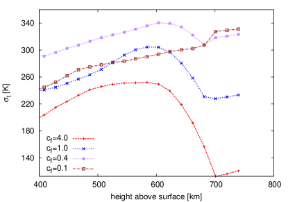
In two-dimensional numerical experiments we found that the value $c_{\rm f}=4.0$ leads to a very slow change in $\langle\epsilon\rangle_{0}$. We ran a simulation with $c_{\rm f}=4.0$ until convection was fully developed. From this point, we started the simulations with several values of $c_{\rm f}$ and relaxed them over half an hour. Subsequently, they were averaged over another half an hour simulation time. The (temporal) standard deviation of the mean temperature stratification $\sigma_{t}$ of these models,

$$\sigma_{t}\left(T\right)(x)=\langle\left[\langle T\rangle(x)-\langle\negthinspace\langle T\rangle\negthinspace\rangle_{t}(x)\right]^{2}\rangle_{t},$$ (17)

where $\langle T\rangle$ is the horizontal and $\langle\negthinspace\langle T\rangle\negthinspace\rangle_{t}$ the temporal and horizontal average of the temperature $T$, is plotted in Figure 1.

The rightmost three grid points in this figure show the boundary layers. A value of $c_{\rm f}=4.0$ decreases the variation to an undesirably small level at the top, which eventually leads to an unrealistic bump in the average $T(\tau)$ relation for layers near the top boundary due to a forced slow relaxation, whereas $c_{\rm f}=0.1$ leads to much stronger variations in the same region. We suggest to use a value of $c_{\rm f}\approx 0.4$ or less. Overall, the effect of $c_{\rm f}$ on the mean temperature stratification throughout the model domain is quite small and restricted to the upper layers of the simulation starting around $250\,{\rm km}$ above the surface. Nevertheless, the choice of large $c_{\rm f}$ can hinder a fast relaxation to a different statistically stationary temperature structure. On the other hand, very small values of $c_{\rm f}$ may lead to strong variations in the temperature which can decrease the numerical stability of the boundary condition. The value of $c_{\rm f}=0.4$ suggested here leads to reasonably fast time scales while keeping the simulation stable for the solar case. We do not expect this choice of $c_{\rm f}=0.4$ to be universal, and recommend to reassess it for other stellar parameters.

Figure 1: Vertical profiles of $\sigma_{t}$, quantifying the temporal variation of the mean temperature (see (17)), obtained for different values of $c_{\rm f}$ as defined in (4e).

3.2 Bottom Boundary Conditions

We compare three 3D solar models with the same simulation setup and different boundary conditions. The simulation boxes extend to $5.2\,{\rm Mm}$ in the vertical and $9.0\,{\rm Mm}$ in the horizontal direction. In the vertical direction, the resolution is $15.3\,{\rm km}$ whereas in the horizontal directions, we chose a resolution of $32.1\,{\rm km}$. The stellar surface is at a geometrical depth of around $0.6\,{\rm Mm}$ to $0.7\,{\rm Mm}$ from the top of the simulation box. For the radiative transfer equation, we use the grey approximation in the upper 30 % of the box, corresponding to a geometrical depth of around $1.6\,{\rm Mm}$, and the diffusion approximation elsewhere.

Model 2 using the BC 2 as in Vögler et al. (2005) was initialised with a one-dimensional profile and an initial perturbation. After two hours of simulation time, the total kinetic energy reached a quasi-constant state, and we considered the model to be relaxed. Models 3a and 3b using the boundary conditions BC 3a and BC 3b, respectively, were started from later snapshots of Model 2. After two additional convective turnover times, we started the production runs. All production runs cover one hour. In Table 1, the boundary conditions used for these models are summarised.

name	type	detailed description	equations	time scales $\left[{\rm h}\right]$	parameters
BC 1	closed	Muthsam et al. (2010a)	(3b)
BC 2	open	Vögler et al. (2005)	(9), (5) & (13)	$\tau_{\rm KH}\approx 550$
BC 3a	open	similar to Freytag et al. (2012)	(9), (8), (11) & (2.1.3)	$\tau_{\rm S}\approx 1000$	$\delta_{p}=1.0$
BC 3b	open		(9), (8), (11) & (2.1.3)	$\tau_{\rm S}\approx 100$	$\delta_{p}=0.1$

Table 1: Summary of bottom boundary conditions in ANTARES. In the fourth column, we refer to the equations constituting these boundary conditions. The time scales are approximate values since they are set in units of sound crossing times in the program.

3.2.1 Time Scales

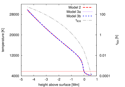
The radiative flux at the top of the domain depends on the amount of energy flowing through the simulation domain. The idea of formula (20) in Vögler et al. (2005), i.e. eq. (5) in this paper, therefore is to correct the (unknown) entropy of the inflow at the bottom boundary according to the radiative flux at the top of the domain until the radiative flux has reached the desired value. The correction works on the Kelvin–Helmholtz time scale $\tau_{\rm KH}$. $\tau_{\rm KH}$ increases rapidly with box depth, as shown in Figure 2. For our standard simulations of solar surface granulation with a domain reaching three to five ${\rm Mm}$ below the stellar surface, $\tau_{\rm KH}\approx 100\,{\rm h}$ to $600\,{\rm h}$. In contrast, the time scale for the surface granulation is several minutes.

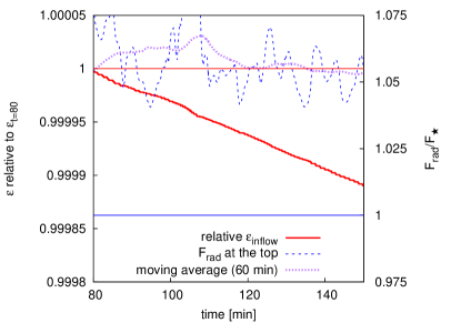
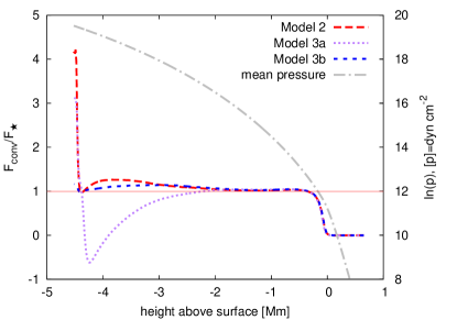
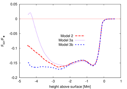
In Figure 3, the radiative flux at the top of the domain of Model 2 and $\epsilon_{\rm inflow}$ calculated with (5) are plotted. It is obvious from Figure 3 that the correction at the bottom boundary does not influence the radiative flux at the top of the domain during the time span covered by the simulation. But the increasingly strong correction leads to exorbitant changes and pathological energy fluxes, as shown in Figs. 4 and 5. We note that the time span covered by the simulation is less than $1\,\%$ of $\tau_{\rm KH}$.

$\tau_{\rm KH}$, the time scale of the correction, is around $600\,{\rm h}$ in Model 2. We can expect that after this time, the correction at the lower boundary will affect the radiative flux at the top of the domain. But performing simulations for such long times is not feasible with today’s computational resources. Common time scales in simulations of solar and stellar surface granulation are much shorter. The formulae (5) and (7) require a much longer relaxation time of the model to be effective. Therefore, we refrain from using this kind of corrections.

We note here that the simulations presented in Vögler et al. (2005) have much more shallow domains with a vertical extent of typically just $1.4\,{\rm Mm}$ of which only $0.8\,{\rm Mm}$ are located below a mean depth for which the optical depth is $1$. As a result, in their case $\tau_{\rm KH}\approx 1$ to $2\,{\rm h}$. For this special case we can expect a much tighter coupling of bottom boundary and $F_{\rm rad}^{\rm top}$ than we observe here for our much deeper models because the distance between the bottom boundary and the stellar surface is only about two pressure scale heights in which case a correction procedure as given by (5) can still be effective.

Figure 2: Temperature stratification of of Models 2, 3a and 3b, and $\tau_{\rm KH}$ as a function of depth. The effect of the boundary conditions on the mean stratification is rather small, at least after one hour of simulation time. The red horizontal line indicates the effective temperature.

Figure 3: Effect of calculating $\epsilon_{\rm inflow}$ by (5) as in Model 2 (red line). The radiative flux $F_{\rm rad}^{\rm top}$ is calculated as horizontal average of $F_{\rm rad}$ in layer $1$ and normalised by the nominal (desired) flux $F_{\star}=\sigma T_{\rm eff}^{4}$. The red horizontal line indicates the initial value of $\epsilon_{\rm inflow}$, and the blue horizontal line the nominal flux $F_{\star}$. $\tau_{\rm KH}=600\,{\rm h}$ for this model.

Figure 4: Convective flux of Models 2, 3a and 3b normalised by $F_{\star}=\sigma T_{\rm eff}^{4}$. The mean pressure profile from Model 2 is shown, too (the pressure profiles of the models do not differ significantly). The boundary conditions affect the lower $2\,{\rm Mm}$, or two pressure scale heights, of the domain. All time averages cover one hour of simulation time.

Figure 5: Kinetic flux of Models 2, 3a and 3b normalised by $F_{\star}=\sigma T_{\rm eff}^{4}$. For Model 3a, the kinetic flux changes sign indicating that the region covered by downflows is larger than the one covered by upflows.

Instead, we decided to set the inflowing entropy by formula (8) such that total flux at the lower boundary $F_{\rm tot}^{\rm bot}$ equals the nominal (desired) flux $F_{\star}=\sigma T_{\rm eff}^{4}$. In Models 3a and 3b, we use the boundary conditions BC 3a and BC 3b as specified in Table 1 which differ in their choice of $\tau_{\rm S}$ and $\delta_{p}$.

Figure 6: Effect of calculating $S_{\rm inflow}$ with (8) and $\tau_{\rm S}=1000\,{\rm h}$ as in Model 3a (red line). The radiative flux $F_{\rm rad}^{\rm top}$ is calculated as horizontal average of $F_{\rm rad}$ in layer $1$. $F_{\rm rad}$ and $F_{\rm tot}^{\rm bot}$ are normalised by $F_{\star}=\sigma T_{\rm eff}^{4}$. The red horizontal line indicates the initial value of $S_{\rm inflow}$, and the blue horizontal line the nominal flux $F_{\star}$.

Figure 7: Effect of calculating $S_{\rm inflow}$ with (8) and $\tau_{\rm S}=100\,{\rm h}$ as in Model 3b (red line). The radiative flux $F_{\rm rad}^{\rm top}$ is calculated as horizontal average of $F_{\rm rad}$ in layer $1$. $F_{\rm rad}$ and $F_{\rm tot}^{\rm bot}$ are normalised by $F_{\star}=\sigma T_{\rm eff}^{4}$. The red horizontal line indicates the initial value of $S_{\rm inflow}$, and the blue horizontal line the nominal flux $F_{\star}$.

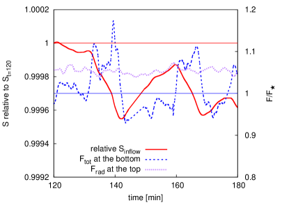
$\tau_{\rm S}$ must be set according to the time scale on which $F_{\rm tot}^{\rm bot}$ changes. As can be seen in Figure 6, the value of $1000\,{\rm h}$ chosen for $\tau_{\rm S}$ in Model 3a is much too large. The change in entropy is too slow to keep $F_{\rm tot}^{\rm bot}$ at the desired level. The resulting convective and kinetic fluxes are pathological, as can be seen in Figs. 4 and 5. On the other hand, the correction works perfectly with $\tau_{\rm S}=100\,{\rm h}$ as shown in Figure 7 for Model 3b. The overall changes in entropy and energy fluxes are small, and the resulting mean fluxes are reasonable.

In Figure 2, we show the temperature profile of these models. The influence of the drastic changes in the boundary conditions and in the energy fluxes is hardly visible on this time scale, but will increase with time. In any case, we prefer BC 3b as used in Model 3b, since these boundary conditions keep the energy fluxes in the lower part of the domain at the desired level and do not produce any serious artifacts even if the initial value of $S_{\rm inflow}$ is not chosen very well.

3.2.2 Dependence on Parameters of the Boundary Conditions

The parameter $\delta_{p}$ in Freytag et al. (2012) defines a time scale on which pressure fluctuations at the bottom boundary are damped. $\tau_{\rm S}$ controls the time scale on which $S_{\rm inflow}$ is changed. Models 3a and 3b differ only in the values chosen for these parameters: for Model 3a, we set $\delta_{p}=1.0$ and $\tau_{\rm S}\approx 1000\,{\rm h}$. For Model 3b, $\delta_{p}=0.1$ and $\tau_{\rm S}\approx 100\,{\rm h}$. Both use the formula (8) for the calculation of $S_{\rm inflow}$. Model 2 uses BC 2.

Figure 8: Velocity distribution $0.25\,{\rm Mm}$, $2.16\,{\rm Mm}$ and $4.45\,{\rm Mm}$ below the stellar surface (from top to bottom). The lowermost layer is only $0.1\,{\rm Mm}$ above the lower boundary and therefore strongly influenced by the boundary conditions. For these pictures, the velocities in each of the layers were grouped into $96$ equal-sized bins. The range of the bins depends on the maximum vertical velocity in this layer. Then, the distribution function was normalised by the number of nodes and time steps such that the total sum is $1$. Due to the coordinate system chosen for ANTARES upflows imply $u(x,y,z)<0$.

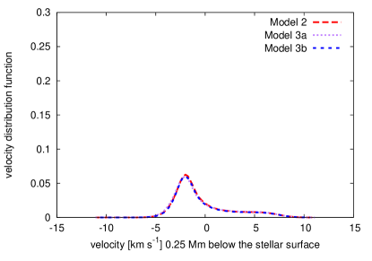
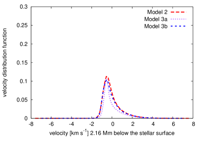
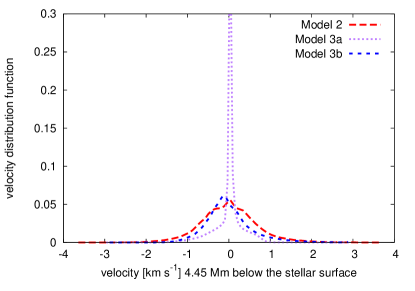
In Figure 8, we show the distribution of the vertical velocity of the three models at three depths. At the depth shown in the top panel of Figure 8, which is situated $0.25\,{\rm Mm}$ below the stellar surface, the differences between the three models are very small. As expected, the distribution has a significant skewness due to the asymmetry between the faster, narrow and turbulent downflows and the slower, more uniform upflows. Note the shift of the maximum induced by the broad upflows (and the fully compressible treatment of the flow). Going deeper and therefore closer to the bottom boundary the differences between the models become more prominent. In the bottom panel, the distribution of Model 3a has much narrower tails and its skewness is much smaller than in Model 2 or Model 3b, whereas the velocity distribution of Model 2 and Model 3b is in all three layers very similar (as we expect it to be). On the other hand, there are some deviations visible for Model 2 while for Model 3b, the distribution is almost invariant as a function of depth apart from a gradual broadening observed for layers farther away from the stellar surface. By modifying only two parameters in the bottom boundary conditions, we changed the velocity distribution of Model 3a in the lower third of the simulation domain considerably: the distribution approaches a narrow Gaussian one with a very flat, additional tail and, in the end, resulting in a small and positive kinetic energy flux.

Comparing our results with the data from Stein et al. (2009), who performed simulations of the upper part of the solar convection zone in boxes of up to $20\,{\rm Mm}$ depth, we conclude that there is no physical reason for the kinetic flux to go to $0$. On the contrary, it should even slightly increase in magnitude when going deeper down into the convection zone — even though that trend in the kinetic flux in the lower part of their simulation box may also be influenced by their boundary conditions.

Furthermore, we conclude from Figure 3 in Stein et al. (2009), that the asymmetry between up- and downflows persists when going deeper into the convection zone, while simultaneously the dominant horizontal scale of the convection increases. This means that the velocity distribution function with depth should have similar shapes.

Returning to the differences between Model 2 and Model 3b, in the bottom panel of Figure 8, the distribution of velocities in Model 2 is closer to symmetric at the bottom, whereas for Model 3b, the asymmetry is less affected by the boundary. The same can also be observed when comparing more shallow models such as those summarised in Table 3. What we observe for Model 3b is hence in agreement with Stein et al. (2009), which is not the case for Models 2 and 3a as their behaviour as a function of depth may be modified by just changing the depth of the simulation box. Therefore boundary condition BC 3b is the best choice among the three models we investigated.

Individual testing of the parameters $\tau_{\rm S}$ and $\delta_{p}$ would have not been affordable in terms of computation time. Anyway, the combination of $\tau_{\rm S}\approx 100\,{\rm h}$ and $\delta_{p}=0.1$ as in BC 3b yields sensible results and we choose them as new default values for these parameters.

3.3 Dependence on Initial Model

In the following, we compare three solar 3D models which differ only in their initial conditions, three different 1D solar structure models. model S from Christensen-Dalsgaard et al. (1996) combines an MLT model of convection (Böhm-Vitense, 1958) with $\alpha_{\rm MLT}=1.99$ used to compute the solar envelope with a semi-empirical model for the photosphere. This model has been calibrated by its authors to match the observed solar radius and luminosity of the Sun at its present age. Moreover, it reproduces the depth of the solar convection zone as inferred from helioseismology (Rosenthal et al., 1999). It is our standard initial model and was used for all simulations of solar surface convection in this paper unless explicitly mentioned. The second and third one are purely theoretical models. They are calculated with the CESAM code (Morel, 1997; Morel and Lebreton, 2008) and use the grey Eddington approximation for the photosphere. The implementation of the convection model of CESAM is described in Samadi et al. (2006). In the second model, convection is modelled by means of an MLT model with $\alpha_{\rm MLT}=1.766$. The third one uses the CGM model of convection (Canuto et al., 1996) with $\alpha_{\rm CGM}=0.69$. All differences between the models are summarised in Table 2.

Since the 1D structure models do not reach high enough into the atmosphere, we extended the 1D models to cover the $4\,{\rm Mm}$ vertical extent of our simulations with $\sim 700\,{\rm km}$ above the stellar surface. All our 3D simulations treat radiative transfer with the opacity binning method with $4$ bins and were relaxed for $80$ to $90\,{\rm min}$ with a vertical resolution of $20\,{\rm km}$. Then, the resolution was increased to about $11\,{\rm km}$ in the vertical and $35\,{\rm km}$ in the horizontal directions. After two sound crossing times, we started the production run with a duration of $30\,{\rm min}$. All 3D simulations use the open boundary conditions BC 3b at the bottom, the LLNL equation of state (Rogers et al., 1996), the non-grey opacities from Kurucz (1993a, b) and the opacity data from Iglesias and Rogers (1996) for the deep interior. For the composition of Grevesse and Noels (1993), we confirmed a good agreement between our choices of atmospheric and interior opacities in the transition region where $\tau\sim 1000$ and $T\sim 10{,}000\,{\rm K}$.

model	atmosphere	convection	$\alpha$	$S_{\rm bot}$	$X$	$Y$	$Z$	$L_{x}$	$L_{P}$
				$10^{9}\cdot\left[{\rm erg}\,{\rm g}^{-1}\,{\rm K}^{-1}\right]$				$\left[{\rm Mm}\right]$	$\left[{\rm Mm}\right]$
model S	semi-empirical	MLT	$1.99$	$1.77355$	$0.7373$	$0.2427$	$0.0200$	$4.07$	$0.75$
CGM	Eddington	CGM	$0.69$	$1.77760$	$0.7381$	$0.2438$	$0.0181$	$4.09$	$0.77$
MLT	Eddington	MLT	$1.766$	$1.77680$	$0.7381$	$0.2438$	$0.0181$	$4.04$	$0.72$

Table 2: Differences in convection and atmosphere model as well as composition for the three models from Section 3.3. We also give the vertical box length $L_{x}$ as well as $L_{P}$, the height of the region where $\langle T\rangle<T_{\rm eff}$. At the beginning of the simulation, $S_{\rm inflow}$ is initialised by the entropy of the initial model at the position of the lower boundary denoted by $S_{\rm bot}$ in this table.

As depicted in Figure 9, the initial entropy profiles differ mainly in the layers from $1\,{\rm Mm}$ below the surface up to the surface itself. At the bottom boundary, the differences in entropy are much smaller. Immediately below the superadiabatic peak, the three profiles from the relaxed simulations, however, are very similar to the CGM initial model. As they do not differ considerably from each other, only one simulation profile is shown in Figure 9. Since $\tau_{\rm KH}$ is about $1$ to $2\,{\rm h}$ in this region, the relaxation time was long enough to allow the simulations to adjust to a common stratification. Near the surface, the simulation results differ from all three one-dimensional models.

In the right panel of Figure 9 where the mean entropy profile is plotted over mean logarithmic pressure, we clearly observe the elevation of the optical surface in the fully developed three dimensional simulation (Nordlund and Stein, 1999). The simulation profile is shifted by about one pressure scale height compared to the MLT and model S profile. Figure 10 demonstrates how this leads to a similar shift upwards for the peak of superadiabicity $\nabla-\nabla_{\rm ad}$ (cf. Kim and Chan 1998). $\nabla-\nabla_{\rm ad}$ in the SAL as shown in Figure 10 is very steep for the CGM initial model. Therefore, the CGM model is able to yield an entropy profile close to the one from the simulations in the interior, while the profile of the simulation above the SAL is closer to that of the MLT model.

Figure 9: Entropy of the three initial models (model S, CGM, MLT) and of the relaxed numerical simulation as well as $\tau_{\rm KH}$ as a function of depth (left) and of the natural logarithm of pressure (right). Since the simulations based on these initial conditions all feature similar relaxed profiles, only one representative simulation is shown in its relaxed state, too. On the left, all curves are aligned such that the region where $\langle T\rangle=T_{\rm eff}$ coincides.

Figure 10: $\nabla-\nabla_{\rm ad}$ of the three initial models and of the numerical simulation as discussed in Fig. 9. The integration rule from Carlson (1963) was used for the angular integration in the radiative transfer solver. The logarithmic temperature gradient $\nabla$ is computed with respect to the total (i.e. including turbulent) pressure. On the left, all curves are aligned such that the region where $\langle T\rangle=T_{\rm eff}$ coincides.

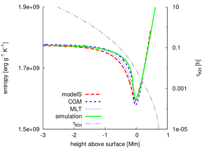
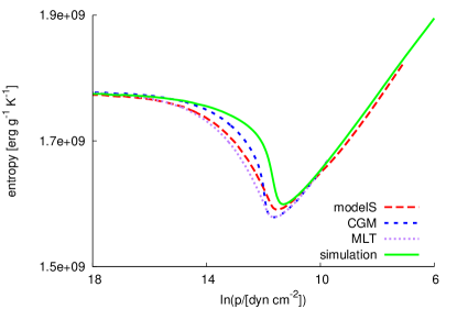
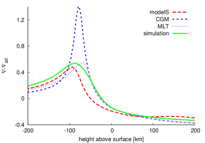
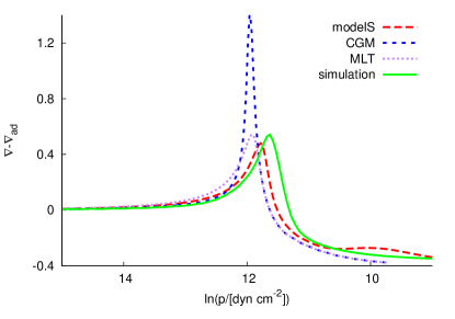
In all three models, once relaxed, the entropy profile as well as the radiative flux at the top do not differ significantly from each other. Thus, differences in the SAL exhibited by the initial models are not important, if the simulations are run long enough in terms of $\tau_{\rm KH}$ for that region. From Figure 9 we deduce that $\tau_{\rm KH}$ is about $1$ to $2\,{\rm h}$ in the region where the entropy profiles of the initial models differ, which corresponds to the simulation time used for relaxation. We return to the role of $\tau_{\rm KH}$ in Section 4.

3.4 Resolution Dependence

Since model S provides the correct adiabat for the solar case, we can expect our simulations to reproduce $T_{\rm eff}$ of the Sun. Therefore, we can use the criterion $T_{\rm eff}=T_{\rm eff,\odot}$ as necessary condition for the correctness of our models. From numerical experiments we deduce that the vertical resolution directly influences $T_{\rm eff}$ of the numerical model. A numerical resolution of at least $10$ to $11\,{\rm km}$ is necessary for this purpose, if the integration rule of Carlson (1963) is used for the angular integration. These numbers are slightly different depending on the type of binning used for the radiative transport, and depend also on the quadrature formula used to perform angular integration.

The resolution dependence is demonstrated in Table 3, where a few grey and non-grey models are compared with respect to the radiative flux at the top of the domain, including Models 2, 3a and 3b from Section 3.2. The other models differ compared to them in terms of simulation domain size, duration of the simulation and grid resolution. Grid resolution, box size, the geometrical depth where the stellar surface is situated, and the bottom boundary conditions are specified in Table 3. All models are three-dimensional and the radiative transfer equation is solved along $24$ rays using the quadrature rule of Carlson (1963) for the angular integration, but the number of bins differs. The grey approximation corresponds to the case of one bin, whereas the non-grey models were calculated with four bins. Details can be found in C and Muthsam et al. (2010a).

In the grey case, $F_{\rm rad}^{\rm top}$ is slightly lower than in the non-grey case where we used $4$ bins (cf. models with a vertical resolution of $11.0\,{\rm km}$ and $13.0\,{\rm km}$, respectively, corresponding to a difference in $T_{\rm eff}$ between $48\,{\rm K}$ and $55\,{\rm K}$). $F_{\rm rad}^{\rm top}$ strongly depends on the vertical resolution. We emphasize that the rate of change of $F_{\rm rad}^{\rm top}$ with numerical resolution depends on the angular quadrature rule. The rule by Carlson (1963), which does not include a vertical ray, requires a very high resolution to yield the correct radiative flux (only the non-grey model with $6.5\,{\rm km}$ vertical resolution yields a $T_{\rm eff}$ very close to the solar one).

Conversely, the dependence of $F_{\rm rad}^{\rm top}$ on the lower boundary conditions is weak on the time scales of these simulations. Table 3 does not show any systematic difference with respect to the bottom boundary conditions. Changes due to boundary effects occur only on much longer time scales.

We note that the horizontal resolution of all simulations presented here is sufficient to get the correct effective temperature and radiative flux at the top of the domain (cf. Asplund et al. 2000; Robinson et al. 2003).

opacities	$\Delta x$	$\Delta y$	$L_{x}$	$L_{y}$	$L_{P}$	b. c.	$T_{\rm eff}$	$S_{\rm bot}$	$S_{\rm bot}-S_{\rm min}$
	$\left[{\rm km}\right]$		$\left[{\rm Mm}\right]$				$\left[{\rm K}\right]$	$10^{9}\cdot\left[{\rm erg}\,{\rm g}^{-1}\,{\rm K}^{-1}\right]$
grey	$19.5$	$40.0$	$4.0$	$6.0$	$0.63$	BC 2	$5959.8$	$1.77131$	$0.16418$
grey	$13.0$	$40.0$	$4.0$	$6.0$	$0.65$	BC 2	$5835.8$	$1.77179$	$0.17576$
grey	$13.0$	$40.0$	$4.0$	$6.0$	$0.65$	BC 3b	$5834.7$	$1.77167$	$0.17546$
grey	$11.0$	$35.3$	$4.1$	$6.0$	$0.74$	BC 3b	$5813.7$	$1.77219$	$0.17800$
non-grey	$13.0$	$40.0$	$4.0$	$6.0$	$0.66$	BC 3b	$5884.2$	$1.77095$	$0.17296$
non-grey	$11.0$	$35.3$	$4.0$	$6.0$	$0.66$	BC 3b	$5868.1$	$1.77065$	$0.17325$
non-grey	$6.5$	$20.0$	$4.0$	$6.0$	$0.68$	BC 2	$5765.3$	$1.77015$	$0.18086$
Model 2	$15.3$	$32.1$	$5.2$	$9.0$	$0.65$	BC 2	$5850.2$	$1.77203$	$0.17379$
Model 3a	$15.3$	$32.1$	$5.2$	$9.0$	$0.65$	BC 3a	$5853.5$	$1.77252$	$0.17409$
Model 3b	$15.3$	$32.1$	$5.2$	$9.0$	$0.65$	BC 3b	$5853.9$	$1.77277$	$0.17451$

Table 3: Effective temperature calculated from $F_{\rm rad}^{\rm top}=\sigma T_{\rm eff}^{4}$ in dependence of binning method, numerical resolution and boundary conditions. $\Delta x$ is the grid spacing and $L_{x}$ the box length in the $x$ (vertical) direction, $\Delta y$ and $L_{y}$ in the $y$ direction. Note that $\Delta z=\Delta y$ and $L_{z}=L_{y}$ in all cases. $L_{P}$ is the height of the region where $\langle T\rangle<T_{\rm eff}$. In addition, the entropy at the bottom of the computational domain and the entropy jump is given. The observed effective temperature of the Sun is $5777.6\,{\rm K}$. Boundary conditions are explained in Table 1. We also show the values for the three models from Section 3.2 which use the grey approximation for radiative transfer.

3.5 Comparison with Closed Boundary Conditions

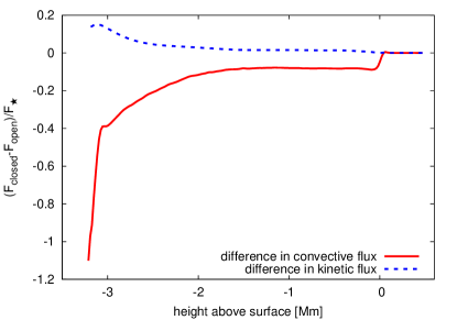
In Figure 11, the energy fluxes of two similar models, one with closed boundaries BC 1 and one with open boundaries BC 3b, are compared. The time average extends over two hours for the model with closed boundaries, and over one hour for the model with open ones. Since the resolution of the model with open boundary conditions was higher ($11.0\,{\rm km}$ vs. $19.4\,{\rm km}$ in the vertical direction), the data was interpolated to the coarser grid of the model with closed boundaries. The resolution changes the radiative flux near the surface, similarly to what was shown in Table 3, thus explaining the step in $F_{\rm conv}$ near a height of $0\,{\rm km}$. In the following, we only discuss the differences in the kinetic and convective fluxes.

The closed boundary conditions force a zero convective and zero kinetic energy flux at the boundaries. Compared to the model with open boundary conditions the convective and the kinetic flux stay smaller in magnitude — keeping in mind their opposite sign. This can be explained by considering the fact that the numerical resolution of the model with closed boundary conditions is rather coarse leading to a wrong radiative flux, and that the top boundary is quite close to the stellar surface.

Forcing the vertical velocities to $0$ at the bottom boundary influences the energy fluxes on about two pressure scale heights. The effect on the kinetic energy flux is smaller than on the convective flux. Around $1\,{\rm Mm}$ above the bottom boundary, the kinetic energy flux from the model with closed boundaries reaches a saturated state with very small differences to the model with open boundaries.

Figure 11: Difference in the energy fluxes of a model with closed and a model with open boundary conditions normalised by $F_{\star}=\sigma T_{\rm eff}^{4}$.

3.6 Two–Dimensional Models

As demonstrated in Figures 3, 6, 7 and 9, thermal relaxation of a simulation takes place on Kelvin–­Helmholtz time–scale of the simulation (Kupka, 2009b). Much care should therefore been taken in setting up the initial state of a simulation, which should be close to the relaxed, statistical steady state. This is most important for the deepest parts of the simulation where the Kelvin­–Helmholtz time scale is long. Thus, if a good initial model is not available, a three-dimensional simulation may not be run long enough with reasonable effort such that it can thermally relax properly.

Since the computational costs for a two-dimensional model are much lower, one is tempted to relax the model in two dimensions first and switch to three dimensions as soon as the correct amount of energy is contained in the simulation domain. Unfortunately, we have found that two- and three-dimensional models of solar surface convection behave quite differently during relaxation.

In Figure 12, the time evolution of the total kinetic energy $E_{\rm kin}$ scaled by the sum of kinetic and thermal energy of a two- and a three-dimensional simulation both starting from the same one-dimensional model is shown. In theory, the kinetic energy should saturate as soon as the convection is fully developed, and the simulation should reach a quasi-stationary state. Obviously, this happens quite rapidly in the three-dimensional case, whereas the kinetic energy of the two-dimensional model starts to oscillate with a very high amplitude and without showing any signs of saturation.

Figure 12: Temporal evolution of the normalised total kinetic energy for a two- and a three-dimensional simulation.

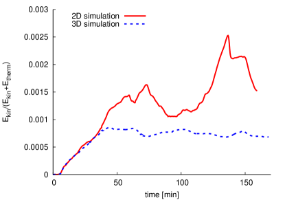
From Figure 12 we deduce that a two-dimensional simulation intended as a precursor of a three-dimensional simulation should be conducted only for a few first sound crossing times. Even then, it can be hard to get rid of the artifacts of the two-dimensionality, especially if the model reaches deep into the convection zone. When we tried to convert a two-dimensional model which was run for a long time (around $60$ sound crossing times) to a three-dimensional one, we encountered serious problems destroying the symmetry in the third dimension in the deeper layers, and the relaxation to a truly three-dimensional state was not shorter than when the model were started directly from the one-dimensional initial model. On the contrary, the model inherits a lot of the deficiencies of the two-dimensional model such as statistical non-stationarity and an overall higher vorticity.

Asplund et al. (2000) pointed out that a two-dimensional simulation of solar granulation leads to different stratifications than a three-dimensional simulation and that the results from two-dimensional simulations are qualitatively wrong concerning line profiles and element abundances. Furthermore, they emphasized that two- and three-dimensional simulations need different values for the entropy of the inflowing material (about $2\%$ difference) to reach the desired effective temperature. As a consequence, it appeared advisable to us to avoid using two-dimensional simulations for testing the bottom boundary conditions since the resulting entropy profiles will differ from their three-dimensional counterparts.

Nevertheless, pre-computing a model in two dimensions can be useful if the two-dimensional phase does not take too long, and if the model is shallow such that the time scale of motion at the bottom boundary is still quite short. For instance for the solar case, the first hour after starting from the one-dimensional initial model may be calculated in two dimensions, if the model is not deeper than $4\,{\rm Mm}$.

Figure 12 furthermore demonstrates that the thermal stratification of a model is quite robust against kinetic motions since the kinetic energy reaches only about $0.1\%$ of the thermal energy. This ratio is comparable to the ratio of $\tau_{\rm sound}$ to $\tau_{\rm KH}$ and thus essentially the time scale of convective transport relative to the time scale of simulation relaxation from our “arbitrary” initial conditions (see Sect. 4).

Confirming the results from Section 3.3 convective motions would need a long time to change the thermal stratification of the entire model, especially since quasi-adiabaticity keeps the sizes of the fluxes of kinetic energy and enthalpy within the same order of magnitude. A significantly different stratification could of course lead to a higher total flux which in turn could reduce the relaxation time somewhat. Still, a good starting model is an essential prerequisite for cost efficient numerical simulations.

In Figure 13 another difference between two- and three-dimensional simulations is shown. There, the relative share of the horizontally averaged turbulent pressure in the innermost boundary layer of the open top boundary condition is plotted. The simulations are the same as in Figure 12. In both cases, $c_{\rm f}=4.0$, but we tested several different values and found no noticeable variation. The difference in the relative contribution of turbulent to total pressure is significant: in the three-dimensional case, it fluctuates around $10\%$ whereas in two dimensions, the turbulent pressure sometimes even exceeds the sum of the gas and the radiative pressure. In the mean, its share is around $30\%$ demonstrating once more the unstable and non-stationary nature of the two-dimensional simulation for the upper layers of the (solar) photosphere.

Figure 13: Temporal evolution of the ratio $p_{\rm turb}/(p+p_{\rm turb})$ in the innermost boundary layer for the same simulations.

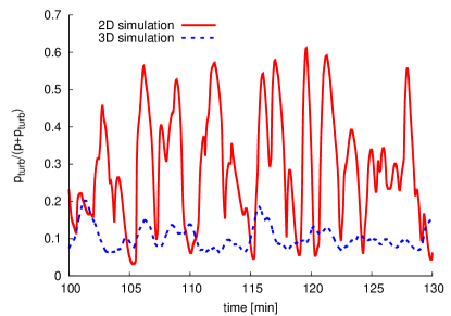
Still, in both cases, the share of the turbulent pressure in the boundary layers is not negligible. Using (4f) is therefore definitely an improvement compared to using the hydrostatic equation without turbulent pressure. Nevertheless, Figure 13 demonstrates that any static approximation of these layers is rather unrealistic.

We note that in comparison with Figure 1.3 (bottom) in Steffen (2000), the difference between two and three dimensions is of a similar magnitude, even though the layer depicted in Figure 13 is even higher in the photosphere than the case represented by the data from Steffen (2000).

4 Discussion

The physical realism of simulations of stellar surface convection depends strongly on the boundary conditions imposed at the top and the bottom of the simulation domain. In a large part of the simulation domain, the flow is influenced in a direct way by the boundary conditions. Therefore, the simulation box must be wide enough in all directions, and the boundary should disturb the velocity field as little as possible. With closed boundary conditions, the motion of the fluid is forced to stop at the boundaries, influencing the dynamics in a large part of the simulation domain (cf. also Kupka and Robinson 2007; Kupka 2009b). Open boundary conditions are clearly preferable as they allow free motion of the fluid, but even with open boundary conditions we recommend to ensure a distance of at least two pressure scale heights between the lower boundary and the SAL.

At the top of the domain, time scales are very short so that effects of the initial stratification are rather short-lived. The effects of the upper boundary are limited by the amount of mass contained there (compared to the rest of the simulation), so locating the top boundary sufficiently far above the optical surface is crucial. The boundary conditions (4h) assume an isoenergetic and hydrostatic stratification, including the effect of turbulent pressure. Since we impose constant velocities with depth in the top boundary layers, waves are not reflected, but transmitted, which increases the long-term stability of the model. The formulation of the top boundary conditions allows variations in the temperature away from the initial profile. In our implementation, the parameter $c_{\rm f}$ controls the stiffness of the open boundary conditions in terms of temporal variations of the temperature, as shown in Figure 1. We found the optimal value by experimentation and it will vary with atmospheric parameters.

The most difficult part in designing open boundary conditions at the bottom of the simulation domain is to specify the internal energy of the inflows. This value controls the overall stratification of a surface convection model by setting the adiabat of the deep (isentropic) convection zone. But the coupling with the energy radiated at the top of the domain operates on time scales which are, for deep, nearly adiabatic convection zones, not feasible to be calculated with multi-dimensional simulations.

For radiative (and conductive) zones a derivation of why $\tau_{\rm KH}$ can be used as an approximation to the thermal adjustment time, which is the actual quantity of interest here, can be found in Chapter 5.3 of Kippenhahn and Weigert (1994), where also limitations of this approximation are pointed out. For the case of convection zones the approximation $\tau_{\rm KH}\approx\tau_{\rm adj}$ is derived in Chapter 6.4 of the same reference as part of a general stability analysis for stellar material at a certain (arbitrary) depth. But for the models considered in Section 3.2, $\tau_{\rm KH}$ is about $6000$ times larger than the convective turn-over time, i.e. the total time for gas to rise from the bottom to the surface, and go back out the bottom boundary of the simulation again. Therefore, a thermal relaxation of the models on $\tau_{\rm KH}$ as intended by formulae (5) and (7) is not affordable with the available computation power. As illustrated with Figure 9, differences in the entropy of the initial model within the superadiabatic region disappear within the local $\tau_{\rm KH}$ whereas the stratification of simulations over shorter relaxation times is determined by the initial model. The success of one-dimensional models in predicting the nearly adiabatic stratification for most but about the upper $1\,{\rm Mm}$ of the solar convection zone is essential for the efficiency of hydrodynamical simulations and for the short relaxation times of 1 to 2 hours of numerical simulation of solar granulation reported in the literature.

For simulations of solar convection, any correction mechanism which correlates the bottom boundary directly with the top boundary will be inefficient, if the simulation box spans more than $1$ or $2\,{\rm Mm}$ of depth below the stellar surface. On the other hand, in shallow simulation boxes the boundary conditions will directly influence the SAL. The simulation box must be large to keep the influence of the bottom boundary small. This, however, prohibits a direct correction mechanism of the entropy at the bottom boundary based on the radiative flux on the top. Instead, the input entropy (resp. internal energy) is much better controlled by a local criterion like (8). We prefer to impose the boundary conditions on the entropy since its value is nearly constant with depth, such that the boundary conditions can be applied at a range of geometrical depths using the same parameter values. Criteria like (5) or (7) can lead to wrong energy fluxes as shown in Figures 4 and 5, since the correction at the bottom does not affect the upper boundary in the time covered by the simulation. In terms of Table 1, our preferred boundary conditions are BC 3b. These boundary conditions allow free in- and outflow with an adiabatic inflow, while fixing the mean mass flux over the bottom boundary to $0$. We refrain from using BC 2 and BC 3a for future simulations.

In the formulation of open boundary conditions, several parameters must be set which influence the behaviour of the flow near the physical boundaries considerably. But, since the computational costs for each single simulation of surface convection are high, systematic tests of the specific effect of each parameter are expensive. Nevertheless, we found a reliable choice for all parameters at least for the solar case, which should be widely applicable to stars of the central and lower main-sequence.

The computational costs cannot be reduced by performing simulations only in two dimensions, since the results differ considerably. As stated also in Asplund et al. (2000), two-dimensional simulations lead to a different stratification and convective velocities since the inherent convective transport properties are different. Furthermore, longer simulation times are needed for statistical significance, since the area coverage of two-dimensional simulations is smaller — which negates the original gain in computational speed. We have found that in addition two-dimensional simulations of solar surface convection do not reach an energetic equilibrium on the same time scale as three-dimensional ones and the upper photosphere is influenced by much stronger fluctuations of turbulent pressure. As the symmetries in the flow-field are also difficult to break by applying a perturbation to initialise a three-dimensional simulation, the use of two-dimensional models as precursors of three-dimensional ones should hence be limited to only five to ten sound crossing times such that the two-dimensional simulation has not yet developed its peculiar thermal stratification and velocity profile. Alternatively, horizontal averages may be used to construct one-dimensional initial models, if the latter cannot be constructed in a reliable way otherwise.

The numerical resolution influences directly the radiative flux at the top of the domain. As we show by numerical experiments in Table 3, the accuracy of the radiative transfer solver can be improved by increasing the numerical resolution on the hydrodynamical grid. If the resolution is sufficiently high, the radiative flux and therefore the effective temperature is in agreement with the observed values. When the angular quadrature rule by Carlson (1963) is used, a vertical grid spacing of at least $10$ to $11\,{\rm km}$ or, preferably, even better than $7\,{\rm km}$, is necessary for the solar case, otherwise the effective temperature of the model will be too high. Therefore, a realistic simulation of surface granulation must be done in sufficiently high resolution. If the aspect ratio of each computational cell is very different from $1$, the magnitude of the intrinsic viscosity of the numerical scheme varies in dependence of the coordinate direction, and surfaces which are inclined with respect to the coordinate system are not well resolved. Therefore, increasing the vertical resolution must be accompanied by an increase in horizontal resolution as well, which makes the simulation much more expensive.

The required spatial resolution depends on the angular integration rule used in the radiative transfer solver. Tanner et al. (2012) discussed that the specific intensity in a fixed grid point is highly variable in time and in the inclination angle. Therefore, choosing a suitable integration rule for the angular dependence of the intensity is crucial to accurately determine the radiative flux, and different formulae will give different results. Only in the limit of more and more ray directions these results will converge.

In contrast to the angular integration rule from Tanner et al. (2012), but also Stein and Nordlund (2003), the integration rule used in our simulations (Carlson, 1963) does not have a vertical ray. But at least in the centre of a granule, the radiative flux is dominated by the vertical direction. If only few rays are used in the angular integration, as it is common in stellar surface convection simulations, a vertical ray should be included in the integration scheme. We will show in a forthcoming paper, how choosing an angular integration rule changes the radiative flux of a numerical simulation of stellar surface convection.

5 Conclusions

In this paper, we investigate the shortcomings of several formulations of open boundary conditions and discuss how to implement boundary conditions for a high-order method which allow realistic simulations of stellar surface granulation.

At the top of the domain, open boundary conditions can transmit waves originating at the stellar surface whereas closed boundaries reflect them. At the bottom boundary, the value of the inflowing entropy must be specified. Some of the proposed approaches, which couple the input flux at the bottom boundary to $F_{\rm rad}$ at the top of the domain (Vögler et al., 2005), work only for shallow boxes where the Kelvin–Helmholtz time scale is small. Also, $F_{\rm rad}$ at the surface of a model is sensitive to the numerical resolution. The initial model determines the stratification of the model, which can only change on the Kelvin–Helmholtz time scale. Open bottom boundary conditions can be expected to excel over closed ones only, if they work on the right time scales, are combined with a suitable, local criterion for the inflow entropy, and if the simulation domain is sufficiently large in all directions. Keeping the inflow entropy variable in time allows control of the total energy flux at the bottom boundary.

The high computational requirements of each single simulation of stellar surface convection prohibits systematic testing of each parameter in the formulation of the open boundary conditions. Nevertheless, we have found a reliable choice for both top and bottom boundaries, i.e. BC 3b from Table 1, which has become the default for numerical simulations of stellar surface convection with ANTARES.

Appendix A Damping Initial Oscillations

Since multidimensional convection models set up from one-dimensional stellar models are not in their lowest energy state, they start to oscillate in the vertical direction (Trampedach et al., 2013). These artifical oscillations differ in amplitude and frequency from the p–mode oscillations expected to be seen in the simulation of stellar surface convection. To remove them, we adapted the procedure described in detail in Trampedach (1997) and Trampedach et al. (2013) in our code. The damping term is an additional term in the velocity equation. The damping velocity $v_{\rm mode}$ is defined by

$$v_{\rm mode}=\frac{\langle\rho u\rangle}{\langle\rho\rangle}.$$ (18)

The (vertical) momentum equation takes the form

$$\frac{\partial\rho u}{\partial t}={\rm rhs\ terms\ from\ eq.~{}\eqref{eq-NS}}-\rho\,\frac{v_{\rm mode}}{t_{\rm mode}},$$ (19)

where $t_{\rm mode}$ is the period of the mode which should be damped. To be consistent, we also added a corresponding term to the total energy equation such that

$$\frac{\partial E}{\partial t}={\rm rhs\ terms\ from\ eq.~{}\eqref{eq-NS}}-\rho u\,\frac{v_{\rm mode}}{t_{\rm mode}},$$ (20)

which improves the stability of this procedure and restores the conservation of energy (even though the conservation errors of the original method are very small). During a production run, we do not apply any damping of vertical momentum.

This procedure can easily be extended to remove dispensable horizontal momenta by replacing the vertical velocity in the calculation of $v_{\rm mode}$ by its horizontal counterparts $v_{{\rm mode},y}$ or $v_{{\rm mode},z}$:

$$v_{{\rm mode},y}=\frac{\langle\rho v\rangle}{\langle\rho\rangle},\ v_{{\rm mode},z}=\frac{\langle\rho w\rangle}{\langle\rho\rangle}.$$ (21)

The time scale $t_{\rm mode}$ can be used to control the rate at which the horizontal momenta are removed. With values of $t_{\rm mode}\approx 1$ sound crossing time, we found that removing of horizontal momenta, if desired, works very efficiently. Even in production runs, we damp the horizontal momenta in the boundary layers to avoid an excessive increase in horizontal momenta.

Appendix B Asymmetric Stencils at the Domain Boundaries

As described in Ferziger and Perić (2002, p. 53), enforcing conditions which set derivatives to zero as in various prescriptions for the in- and outflow at top and bottom boundaries like (4a), (9), or (13) should not be done by simply setting $u$ to a constant value, but by exact inversion of the stencils used for the calculation of the derivatives. Especially, if higher-order methods as, e.g., the fourth order method presented in Happenhofer et al. (2013), are used, unsuitable procedures can lead to pathological behaviour of the velocity field near the boundary.

With a five-point wide stencil, boundary conditions for ANTARES must be set on three vertical layers. As before, all physical layers are numbered from $1$ to $n_{x}$ starting at the top of the simulation box. At the top boundary of the computational domain, derivatives of a scalar-valued function $\phi$ at the cell centres are calculated by

$$\frac{\partial\phi}{\partial x}(x_{-2}) =\frac{-25\phi_{-2}+48\phi_{-1}-36\phi_{0}+16\phi_{1}-3\phi_{2}}{12\Delta x},$$ (22a)

$$\frac{\partial\phi}{\partial x}(x_{-1}) =\frac{-3\phi_{-2}-10\phi_{-1}+18\phi_{0}-6\phi_{1}+\phi_{2}}{12\Delta x},$$ (22b)

following the approach presented in Happenhofer et al. (2013). For $\frac{\partial\phi}{\partial x}(x_{0})$, the symmetric stencil can be used, i.e.

$$\frac{\partial\phi}{\partial x}(x_{0})=\frac{\phi_{-2}-8\phi_{-1}+8\phi_{1}-\phi_{2}}{12\Delta x},$$ (22c)

where $\phi_{i}=\phi(x_{i})$ and mirrored expressions are valid for the bottom boundary. For $\frac{\partial\phi}{\partial x}(x_{\frac{1}{2}})$ and other derivatives at the cell boundary, similar expressions can be calculated with the same procedure.

Expansion in Taylor series shows that the error term $\varepsilon$ is given by

$$\varepsilon\left(\frac{\partial\phi}{\partial x}(x_{-2})\right) =-\frac{1}{5}\left(\Delta x\right)^{4}\phi^{(5)}(\zeta),$$ (23a)

$$\varepsilon\left(\frac{\partial\phi}{\partial x}(x_{-1})\right) =\frac{1}{20}\left(\Delta x\right)^{4}\phi^{(5)}(\zeta),$$ (23b)

$$\varepsilon\left(\frac{\partial\phi}{\partial x}(x_{0})\right) =-\frac{1}{30}\left(\Delta x\right)^{4}\phi^{(5)}(\zeta),$$ (23c)

demonstrating the fourth order of the given stencils. The error constant increases the more the stencils are asymmetric.

If we try to enforce $\frac{\partial\phi}{\partial x}=0$ by setting $\phi_{-2}=\phi_{-1}=\phi_{0}=\phi_{1}$, the derivatives will not be zero numerically. Instead, we solve eqs. (23) for $\frac{\partial\phi}{\partial x}=0$, to get

$$\phi_{-2}= \frac{64}{55}\phi_{1}-\frac{9}{55}\phi_{2},$$ (24a)

$$\phi_{-1}= \frac{63}{55}\phi_{1}-\frac{8}{55}\phi_{2},$$ (24b)

$$\phi_{0}= \frac{64}{55}\phi_{1}-\frac{9}{55}\phi_{2}.$$ (24c)

While this procedure immediately applies to bottom boundary conditions as specified through (5), (6), and (13), for conditions set by (7) or (8), (9) in conjunction with (2.1.3), the vertical velocity $u$ in the innermost boundary layer $n_{x}+1$ is already set by the enforcement of mass conservation (12c). Whereas we can use the procedure from above for the horizontal velocities, the boundary condition for the vertical velocity must be changed to

$$u_{n_{x}+1} \rm{\ set\ to\ enforce\ mass\ conservation},$$ (25a)

$$u_{n_{x}+2}= \frac{279}{197}u_{n_{x}+1}-\frac{99}{197}u_{n_{x}}+\frac{17}{197}u_{n_{x}-1},$$ (25b)

$$u_{n_{x}+3}= \frac{252}{197}u_{n_{x}+1}-\frac{64}{197}u_{n_{x}}+\frac{9}{197}u_{n_{x}-1}.$$ (25c)

Appendix C Calculation of the Energy Fluxes

The calculation of the energy fluxes follows Canuto (1997) which describes the procedure for the case of a perfect gas. We have generalized this to arbitrary equations of state in the following. We also define the residual velocities

$$u^{\prime\prime}=u-\frac{\langle\rho u\rangle}{\langle\rho\rangle},\ v^{\prime\prime}=v-\frac{\langle\rho v\rangle}{\langle\rho\rangle},\ w^{\prime\prime}=w-\frac{\langle\rho w\rangle}{\langle\rho\rangle},$$ (26)

where net mass fluxes have been removed. For fluxes only, we ignore our coordinate convention, and have positive fluxes going out through the top of the box.

C.1 Radiative Flux ($F_{\rm rad}$)

In regions where the optical depth is $\lesssim 100$, the radiative transfer equation is solved with the short characteristics method as described in Muthsam et al. (2010a). The equation is solved by an angular integration over a discrete set of rays. The dependence on the frequency is considered by repeating the calculation several times for averages of intensity over frequency sets, to each of which the weight $\omega_{\rm bin}$ is assigned (Nordlund, 1982; Stein and Nordlund, 2003; Ludwig et al., 1994). In every grid-point of the simulation, the intensity $I({\rm bin},{\rm ray})$ is calculated for $N_{\rm rays}$ rays, where $N_{\rm rays}$ depends on the quadrature formula chosen for the angular integration, and $N_{\rm bins}$ frequency bins (Ludwig et al., 1994). For the integration rule from Carlson (1963) which is used in the simulations presented in this paper, $N_{\rm rays}$ is 24 in three and 12 in two dimensions due to symmetries. In three dimensions, we have three rays per octant with two different angles in latitude and three in the azimuthal direction. $N_{\rm bins}=1$ is the grey approximation, and $N_{\rm bins}=4$ is used for non-grey simulations. The opacity data is taken from Iglesias and Rogers (1996), Ferguson et al. (2005) and Kurucz (1993a, b). For details, we refer to Muthsam et al. (2010a).

The vertical component of the radiative flux is calculated by

$$F_{\rm rad}=\frac{4\pi}{N_{\rm rays}}\sum_{\rm rays}\sum_{\rm bins}\omega_{\rm bin}\,n_{x}\,I({\rm bin},{\rm ray}),$$ (27)

where $n_{x}$ is the vertical component of the ray direction. In optically thick regions, the diffusion approximation is valid and $F_{\rm rad}$ can be calculated simply by

$$F_{\rm rad}=k\,\frac{\partial T}{\partial x}.$$ (28)

The sign of the heat conduction coefficient, $k$, is positive due to the coordinate system chosen in ANTARES.

In our simulations, the transition to the diffusion approximation is done at a fixed geometrical depth. We choose this depth such that the transition is in any case performed in a region where the optical depth in every grid point is between $100$ and $1000$, also in case of optically thin downflows.

C.2 Convective Flux ($F_{\rm conv}$)

The vertical component of the convective flux is defined by

$$F_{\rm conv}=\langle u^{\prime\prime}\rho\left(h-\frac{\langle e+p\rangle}{\langle\rho\rangle}\right)\rangle,$$ (29)

where $h=\frac{e+p}{\rho}$ is the specific enthalpy and $u^{\prime\prime}$ is defined in equation (26).

C.3 Kinetic Flux ($F_{\rm kin}$)

The vertical component of the kinetic flux in three dimensions is defined by

$$F_{\rm kin}=\frac{1}{2}\langle\rho u^{\prime\prime}\left(u^{\prime\prime 2}+v^{\prime\prime 2}+w^{\prime\prime 2}\right)\rangle.$$ (30)

We define this flux with the primed velocities to remove short-lived trends and to make the fluxes meaningful even when computed over short time intervals. When the model is statistically stationary and the averaging interval is long enough, these fluxes coincide with those defined in Nordlund and Stein (2001). Furthermore, the viscous flux is defined as the horizontal average of the viscous stress tensor as in equation (16) from Nordlund and Stein (2001) or equation (7b) in Canuto (1997).

References

- Asplund et al. (2000) Asplund, M., Ludwig, H.-G., Nordlund, A., Stein, R. F., 2000. The effects of numerical resolution on hydrodynamical surface convection simulations and spectral line formation. A&A 359, 669 – 681.
- Beeck et al. (2012) Beeck, B., Collet, R., Steffen, M., Asplund, M., Cameron, R. H., Freytag, B., Hayek, W., Ludwig, H.-G., Schüssler, M., 2012. Simulations of the solar near-surface layers with the CO5BOLD, MURaM, and Stagger codes. A&A 539, A121.
- Böhm-Vitense (1958) Böhm-Vitense, E., 1958. Über die Wasserstoffkonvektionszone in Sternen verschiedener Effektivtemperaturen und Leuchtkräfte. Zeitschrift für Astrophysik 46, 108 – 143.
- Canuto (1997) Canuto, V. M., 1997. Compressible Turbulence. ApJ 482, 827 – 851.
- Canuto et al. (1996) Canuto, V. M., Goldman, I., Mazzitelli, I., 1996. Stellar Turbulent Convection: A Self-consistent Model. ApJ 473, 550 – 559.
- Carlson (1963) Carlson, B. G., 1963. The numerical theory of neutron transport. Vol. 1 (Statistical Physics). Methods in Computational Physics. Advances in Research and Applications, Ch. 1, pp. 1 – 42.
- Cheung (2006) Cheung, C. M. M., 2006. Magnetic flux emergence in the solar photosphere. Ph.D. thesis, Universität Göttingen.
- Christensen-Dalsgaard et al. (1996) Christensen-Dalsgaard, J., Dappen, W., Ajukov, S. V., Anderson, E. R., Antia, H. M., Basu, S., Baturin, V. A., Berthomieu, G., Chaboyer, B., Chitre, S. M., Cox, A. N., Demarque, P., Donatowicz, J., Dziembowski, W. A., Gabriel, M., Gough, D. O., Guenther, D. B., Guzik, J. A., Harvey, J. W., Hill, F., Houdek, G., Iglesias, C. A., Kosovichev, A. G., Leibacher, J. W., Morel, P., Proffitt, C. R., Provost, J., Reiter, J., Rhodes, Jr., E. J., Rogers, F. J., Roxburgh, I. W., Thompson, M. J., Ulrich, R. K., May 1996. The Current State of Solar Modeling. Science 272, 1286 – 1292.
- Ferguson et al. (2005) Ferguson, J. W., Alexander, D. R., Allard, F., Barman, T., Bodnarik, J. G., Hauschildt, P. H., Heffner-Wong, A., Tamanai, A., 2005. Low-Temperature Opacities. ApJ 623, 585.
- Ferziger and Perić (2002) Ferziger, J. H., Perić, M., 2002. Computational Methods for Fluid Dynamics, 3rd Edition. Springer, Berlin.
- Freytag et al. (2012) Freytag, B., Steffen, M., Ludwig, H.-G., Wedemeyer-Böhm, S., Schaffenberger, W., Steiner, O., 2012. Simulations of stellar convection with CO5BOLD. JCP 231, 919 – 959.
- Grevesse and Noels (1993) Grevesse, N., Noels, A., January 1993. Cosmic abundances of the elements. In: Prantzos, N., Vangioni-Flam, E., Casse, M. (Eds.), Origin and Evolution of the Elements. pp. 15 – 25.
- Happenhofer et al. (2013) Happenhofer, N., Grimm-Strele, H., Kupka, F., Löw-Baselli, B., Muthsam, H. J., 2013. A low Mach number solver: Enhancing applicability. JCP 236, 96 – 118.
- Iglesias and Rogers (1996) Iglesias, C. A., Rogers, F. J., 1996. Updated OPAL Opacities. ApJ 464, 943.
- Jacoutot et al. (2008) Jacoutot, L., Kosovichev, A. G., Wray, A., Mansour, N. N., 2008. Realistic Numerical Simulations of Solar Convection and Oscillations in Magnetic Regions. ApJL 684 (1), L51.
- Jiang and Shu (1996) Jiang, G.-S., Shu, C.-W., 1996. Efficient Implementation of Weighted ENO Schemes. JCP 126, 202 – 228.
- Kim and Chan (1998) Kim, Y.-C., Chan, K. L., 1998. A Hydrodynamic Simulation of the Highly Superadiabatic Layer of the Sun. ApJL 496, L121.
- Kippenhahn and Weigert (1994) Kippenhahn, R., Weigert, A., 1994. Stellar Structure and Evolution, 3rd Edition. Springer Berlin, Berlin.
- Kupka (2009a) Kupka, F., 2009a. 3D stellar atmospheres for stellar structure models and asteroseismology. MmSAI 80, 701 – 710.
- Kupka (2009b) Kupka, F., 2009b. Turbulent Convection and Simulations in Astrophysics. Springer Lecture Notes in Physics 756, Ch. 3, pp. 49–105.
- Kupka et al. (2009) Kupka, F., Ballot, J., Muthsam, H. J., 2009. Effects of Resolution and Helium Abundance in A Star Surface Convection Simulations. Comm. in Asteroseismology 160, 30 – 63.
- Kupka et al. (2012) Kupka, F., Happenhofer, N., Higueras, I., Koch, O., 2012. Total-variation-diminishing implicit–explicit Runge–Kutta methods for the simulation of double-diffusive convection in astrophysics. JCP 231, 3561 – 3586.
- Kupka and Robinson (2007) Kupka, F., Robinson, F., 2007. On the effects of coherent structures on higher order moments in models of solar and stellar surface convection. MNRAS 374, 305 – 322.
- Kurucz (1993a) Kurucz, R., 1993a. ATLAS9 Stellar Atmosphere Programs and 2 km/s grid. Kurucz CD-ROM No. 13. Cambridge, Mass.: Smithsonian Astrophysical Observatory.
- Kurucz (1993b) Kurucz, R., 1993b. Opacities for Stellar Atmospheres: [+0.0],[+0.5],[+1.0]. Kurucz CD-ROM No. 2. Cambridge, Mass.: Smithsonian Astrophysical Observatory.
- Lemmerer et al. (2013) Lemmerer, B., Utz, D., Hanslmeier, A., Veronig, A., Thonhofer, S., Grimm-Strele, H., Karyappa, R., 2013. 2D Segmentation of small convective patterns in RHD simulations. Submitted to A&A.
- Ludwig et al. (1999) Ludwig, H.-G., Freytag, B., Steffen, M., 1999. A calibration of the mixing-length for solar-type stars based on hydrodynamical simulations. A&A 346, 111 – 124.
- Ludwig et al. (1994) Ludwig, H.-G., Jordan, S., Steffen, M., 1994. Numerical simulations of convection at the surface of a ZZ Ceti white dwarf. A&A 284, 105 – 117.
- Morel (1997) Morel, P., 1997. CESAM: A code for stellar evolution calculations. Astron. Astrophys. Suppl. Ser. 124, 597 – 614.
- Morel and Lebreton (2008) Morel, P., Lebreton, Y., 2008. CESAM: a free code for stellar evolution calculations. Astrophysics and Space Science 316, 61 – 73.
- Mundprecht et al. (2013) Mundprecht, E., Muthsam, H. J., Kupka, F., 2013. Multidimensional realistic modelling of Cepheid-like variables. I. Extensions of the ANTARES code. MNRAS 435, 3191 – 3205.
- Muthsam et al. (2010a) Muthsam, H. J., Kupka, F., Löw-Baselli, B., Obertscheider, C., Langer, M., Lenz, P., 2010a. ANTARES – A Numerical Tool for Astrophysical RESearch with applications to solar granulation. NewA 15, 460 – 475.
- Muthsam et al. (2010b) Muthsam, H. J., Kupka, F., Mundprecht, E., Zaussinger, F., Grimm-Strele, H., Happenhofer, N., 2010b. Simulations of stellar convection, pulsation and semiconvection. In: Brummell, N., Brun, A., Miesch, M., Ponty, Y. (Eds.), Astrophysical Dynamics: From Stars to Galaxies. No. 271 in Proceedings IAU Symposium. pp. 179 – 186.
- Muthsam et al. (2007) Muthsam, H. J., Löw-Baselli, B., Obertscheider, C., Langer, M., Lenz, P., Kupka, F., 2007. High-resolution models of solar granulation: the two-dimensional case. MNRAS 380, 1335 – 1340.
- Nordlund (1982) Nordlund, A., 1982. Numerical simulations of the solar granulation. I. Basic equations and methods. A&A 107, 1 – 10.
- Nordlund and Stein (1990) Nordlund, A., Stein, R. F., 1990. 3-D simulations of solar and stellarconvection and magnetoconvection. Computer Physics Communications 59, 119 – 125.
- Nordlund and Stein (1999) Nordlund, A., Stein, R. F., 1999. Convection Simulations. In: Gimzénez, A., Guinan, E., Montesinos, B. (Eds.), Theory and Tests of Convection in Stellar Structure. Vol. 173 of ASP Conference Series. pp. 91 – 102.
- Nordlund and Stein (2001) Nordlund, A., Stein, R. F., 2001. Solar Oscillations and Convection. I. Formalism for Radial Oscillations. ApJ 546, 576 – 584.
- Nordlund et al. (2009) Nordlund, A., Stein, R. F., Asplund, M., 2009. Solar Surface Convection. Living Rev. Solar Phys. 6, 1 – 117, cited on January 16, 2013.
- Robinson et al. (2003) Robinson, F., Demarque, P., Li, L. H., Sofia, S., Kim, Y.-C., Chan, K. L., Guenther, D. B., 2003. Three-dimensional convection simulations of the outer layers of the Sun using realistic physics. MNRAS 340 (3), 923 – 936.
- Rogers et al. (1996) Rogers, F. J., Swenson, F. J., Iglesias, C. A., 1996. OPAL Equation-of-State Tables for Astrophysical Applications. ApJ 456, 902.
- Rosenthal et al. (1999) Rosenthal, C. S., Christensen-Dalsgaard, J., Nordlund, A., Stein, R. F., Trampedach, R., 1999. Convective contributions to the frequencies of solar oscillations. A&A 351, 689 – 700.
- Samadi et al. (2006) Samadi, R., Kupka, F., Goupil, M., Lebreton, Y., van’t Veer Menneret, C., 2006. Influence of local treatments of convection upon solar p mode excitation rates. A&A 445, 233 – 242.
- Shu (2003) Shu, C.-W., 2003. High-order Finite Difference and Finite Volume WENO Schemes and Discontinuous Galerkin Methods for CFD. International Journal of Computational Fluid Dynamics 17 (2), 107 – 118.
- Steffen (2000) Steffen, M., 2000. 2D numerical simulation of stellar convection – An overview. In: Cheng, L., Chau, H., Chan, K., Leung, K. (Eds.), Stellar Astrophysics. Proceedings of the Pacific Rim Conference held in Hong Kong, 1999. pp. 25 – 34, available at http://www.aip.de/groups/sternphysik/stp/publications_neu.html.
- Stein and Nordlund (1998) Stein, R. F., Nordlund, A., 1998. Simulations of Solar Granulation. I. General Properties. ApJ 499, 914 – 933.
- Stein and Nordlund (2003) Stein, R. F., Nordlund, A., 2003. Radiative Transfer in 3D Numerical Simulations. In: Hubeny, I., Mihalas, D., Werner, K. (Eds.), Stellar Atmosphere Modeling. Vol. 288 of ASP Conference Proceedings. pp. 519 – 532.
- Stein et al. (2009) Stein, R. F., Nordlund, A., Georgobiani, D., Benson, D., Schaffenberger, W., 2009. Supergranulation–Scale Convection Simulations. In: Dikpati, M., Arentoft, T., Hernández, I. G., Lindsey, C., Hill, F. (Eds.), Solar-Stellar Dynamos as Revealed by Helio- and Asteroseismology. Vol. 416 of ASP Conference Proceedings. pp. 421 – 426.
- Tanner et al. (2012) Tanner, J. D., Basu, S., Demarque, P., 2012. Comparing the Effect of Radiative Transfer Schemes on Convection Simulations. ApJ 759, 120 – 131.
- Tanner et al. (2013) Tanner, J. D., Basu, S., Demarque, P., 2013. Variation of Stellar Envelope Convection and Overshoot with Metallicity. ApJ 767, 78 – 87.
- Trampedach (1997) Trampedach, R., 1997. Convection in Stellar Atmospheres. Master’s thesis, Aarhus University, available at users-phys.au.dk/art/papers/speciale.pdf.
- Trampedach et al. (2013) Trampedach, R., Asplund, M., Collet, R., Nordlund, A., Stein, R. F., 2013. A Grid of 3D Stellar Atmosphere Models of Solar Metallicity: I. General Properties, Granulation and Atmospheric Expansion. ApJ 769, 18.
- Vögler et al. (2005) Vögler, A., Shelyag, S., Schüssler, M., Cattaneo, F., Emonet, T., Linde, T., 2005. Simulations of magneto-convection in the solar photosphere. A&A 429, 335 – 351.
- Wedemeyer-Böhm et al. (2004) Wedemeyer-Böhm, S., Freytag, B., Steffen, M., Ludwig, H.-G., Holweger, H., 2004. Numerical simulation of the three-dimensional structure and dynamics of the non-magnetic solar chromosphere. A&A 414, 1121 – 1137.
- Zaussinger and Spruit (2013) Zaussinger, F., Spruit, H., June 2013. Semiconvection: numerical simulations. A&A 554, A119.