Cosmological Evolution for Dark Energy Models in f​(T)𝑓𝑇f(T) Gravity

M. Sharif and Sehrish Azeem
Department of Mathematics, University of the Punjab,
Quaid-e-Azam Campus, Lahore-54590, Pakistan
msharif.math@pu.edu.pksehrishazeem4@gmail.com
Abstract

In this paper, we investigate the behavior of equation of state parameter and energy density for dark energy in the framework of f​(T)𝑓𝑇f(T) gravity. For this purpose, we use anisotropic LRS Bianchi type I universe model. The behavior of accelerating universe is discussed for some well-known f​(T)𝑓𝑇f(T) models. It is found that the universe takes a transition between phantom and non-phantom phases for f​(T)𝑓𝑇f(T) models except exponential and logarithmic models. We conclude that our results are relativity analogous to the results of FRW universe.

Keywords: f​(T)𝑓𝑇f(T) gravity; LRS Bianchi type I universe; Equation of state; Dark energy.
PACS: 04.50.kd; 98.80.-k.

1 Introduction

The extensions of general relativity seem attractive to explain the late time acceleration of the universe and dark energy (DE). High redshift type Supernova Ia experiments show that the universe is experiencing accelerated expansion in every direction, while the other observations of anisotropies give indirect evidence (Perlmutter et al. 1999; Knop et al. 2003; Riess et al. 1998). The mysterious anti-gravity DE material is smoothly filled in the universe. Dark energy with negative pressure and positive energy density depends on the equation of state (EoS), p=Ο‰β€‹Οπ‘πœ”πœŒp=\omega\rho, where Ο‰πœ”\omega is the function of cosmic time called EoS parameter (Sharif and Zubair 2010a). There are different forms of dynamically varying DE phases related with negative behavior of EoS parameter. The range, βˆ’1<Ο‰<βˆ’1/31πœ”13-1<\omega<-1/3, corresponds to the non-phantom phase of the universe while the phantom phase occurs for Ο‰<βˆ’1πœ”1\omega<-1 (Yadav 2011; Sahni and Starobinsky 2008). Quintom is such a DE model which can cross the phantom divide line Ο‰=βˆ’1πœ”1\omega=-1 from both sides (Khatua et al. 2011; Feng et al. 2005).

The dynamical nature of DE can originate from a variable cosmological constant, phantom as well as scalar field, tachyon, Chaplygin gas and modified gravities (Martinelli and Melchiorri 2009). In spite of all observational evidences, the expanding universe is still a challenging issue in modern physics (Yang et al. 2010). An alternative approach to accommodate the current accelerating expansion of the universe is to modify the GR on large scale, such as, the scalar-tensor theories, f​(R)𝑓𝑅f(R) theory, f​(T)𝑓𝑇f(T) theory and DGP braneword theory (Yang 2011a; Zheng and Huang 2011) etc.

Among these theories, the generalized teleparallel theory of gravity has recently gained a lot of interest due to its possible explanation about DE. In this generalization, the torsion scalar, T𝑇T, is replaced by its general function f​(T)𝑓𝑇f(T) in the Lagrangian of teleprallel gravity (Sharif and Rani 2011a). The f​(T)𝑓𝑇f(T) gravity models use the WeitzenboΒ¨Β¨π‘œ\ddot{o}ck connection which inherits only torsion and responsible for the accelerating expansion of the universe (Myrzakulov 2011). This approach (theory) originally developed by Einstein in 192819281928 under the name ”Fern-Parallelismus” or ”distant Parallelism” or ”teleparallelism” (Linder 2010; Unzicker and Case 2005). The f​(T)𝑓𝑇f(T) theory has significant advantage of its second order field equations as compared to f​(R)𝑓𝑅f(R) theory with fourth order field equations (Sharif and Shamir 2009; Sharif and Kausar 2010, 2011a, 2011b; Jamil et al. 2012a, 2012b).

Bengochea and Ferraro (2009) described the recently detected acceleration of the universe without DE and performed observational viability tests by using recent SNIa data for some f​(T)𝑓𝑇f(T) models. Linder (2010) explored that the cosmological constant is not only the component for the acceleration of the universe. This was also observed through a generalization of GR to other gravity theories. Zhang et al. (2011) discussed the dynamical analysis for the logarithmic and power form of f​(T)𝑓𝑇f(T) models. They investigated phase-space analysis of models, their stability of the critical points and evolution of EoS parameter. In a recent paper, Sharif and Shamaila (2011b) constructed some f​(T)𝑓𝑇f(T) models by using Bianchi type I (BI) universe. They also derived EoS parameter for two modified teleparallel models. Yang (2011b) investigated three new f​(T)𝑓𝑇f(T) models and described their physical implications and cosmological behavior.

Recently, Bamba et al. (2011) discussed different f​(T)𝑓𝑇f(T) models to investigate the cosmological evolutions of EoS parameter for DE and their observational constraints. Wu and Yu (2011) proposed two new f​(T)𝑓𝑇f(T) models and analyzed that the crossing of the phantom divide line is consistent with recent cosmological observational data. Chen et al. (2011) investigated this problem by extending modified gravity at the background and perturbed level. They also explored this theory for quintessence scenario.

One of the predictions from inflation is that the observed universe should nearly isotropic on large scales. Spatially homogenous and isotropic universe can be well described by FRW model which can not be explained the early universe. The existence of anisotropy at early times is a natural phenomenon to investigate the local anisotropies that we observe today in galaxies and cluster. Recent measurements on the cosmic microwave background radiation (CMBR) through WMAP suggest that the anisotropic inflationary models should be considered (Vielva 2004; Costa 2004). In early epoch of the big bang, the universe does not maintain its isotropic behavior at very small scales (Kumar and Singh 2008). In order to get a realistic model representing an expanding, homogenous and anistropic universe, Bianchi type cosmological models are considered. The isotropic behavior of today universe makes BI model a prime candidate for describing the possible anisotropic effects of the early universe on modern day data observations.

Many people worked on simplest anisotropic model called BI universe to discuss the effects of anisotropy in several contexts. Kumar and Singh (2007) developed mechanism for solution of the field equations by considering BI universe model. The same authors (Kumar and Singh 2008) investigated the exact BI solutions which give the constant value of the deceleration parameter in scalar-tensor theory. Recently, Sharif and Waheed (2012) studied exact solutions for anisotropic fluids by taking the locally rotationally symmetric Bianchi Type I (LRS BI) universe model which generalizes the flat FRW universe in the modified theory (BD). There are many papers available in literature where this model has been used widely (Bali and Kumawat 2008; Amirhashchi 2011; Yadav and Saha 2012).

In this paper, we explore cosmological evolution for some well-known f​(T)𝑓𝑇f(T) models by using BI universe. For this purpose, we evaluate the EoS parameter and energy density of DE and display graphically. The paper is organized as follows: In the next section, we review teleparallel theory of gravity. We formulate the field equations of f​(T)𝑓𝑇f(T) gravity and some cosmological parameters for BI universe in section 3. Section 4 is devoted to examine the cosmological behavior of some f​(T)𝑓𝑇f(T) models to check whether the crossing of phantom divide line occurs or not. We summarize and conclude the results in the last section 5.

2 The f​(T)𝑓𝑇f(T) Formalism

Here we briefly review the modified teleparallel theory of gravity. In this theory, the vierbein field hi​(xΞΌ)subscripth𝑖superscriptπ‘₯πœ‡\textbf{h}_{i}(x^{\mu}) at each point xΞΌsuperscriptπ‘₯πœ‡x^{\mu} of the manifold are orthonormal basis, where the Latin (i,j,…=0,1,2,3)formulae-sequence𝑖𝑗…0123(i,j,...=0,1,2,3) and Greek alphabets (ΞΌ,Ξ½,…=0,1,2,3)formulae-sequenceπœ‡πœˆβ€¦0123(\mu,\nu,...=0,1,2,3) are used for the tangent space and spacetime indices respectively. The spacetime metric tensor is defined from the dual vierbein as

gμ​ν=Ξ·i​j​hΞΌi​hΞ½j,subscriptπ‘”πœ‡πœˆsubscriptπœ‚π‘–π‘—subscriptsuperscriptβ„Žπ‘–πœ‡subscriptsuperscriptβ„Žπ‘—πœˆg_{\mu\nu}=\eta_{ij}h^{i}_{\mu}h^{j}_{\nu}, (1)

where Ξ·i​j=d​i​a​g​(1,βˆ’1,βˆ’1,βˆ’1)subscriptπœ‚π‘–π‘—π‘‘π‘–π‘Žπ‘”1111\eta_{ij}=diag(1,-1,-1,-1) is the Minkowski spacetime for the tangent space. For a given metric, there exists infinite tetrad fields hΞΌisubscriptsuperscriptβ„Žπ‘–πœ‡h^{i}_{\mu} which satisfy the following properties (Ferraro and Fiorini 2007; Hayashi and Shirafuji 1979)

hΞΌi​hjΞΌ=Ξ΄ji,hΞΌi​hiΞ½=δμν.formulae-sequencesubscriptsuperscriptβ„Žπ‘–πœ‡subscriptsuperscriptβ„Žπœ‡π‘—subscriptsuperscript𝛿𝑖𝑗subscriptsuperscriptβ„Žπ‘–πœ‡subscriptsuperscriptβ„Žπœˆπ‘–subscriptsuperscriptπ›Ώπœˆπœ‡h^{i}_{\mu}h^{\mu}_{j}=\delta^{i}_{j},\quad h^{i}_{\mu}h^{\nu}_{i}=\delta^{\nu}_{\mu}. (2)

The action for f​(T)𝑓𝑇f(T) theory with matter is given by (Bamba et al. 2011)

I=116​π​Gβ€‹βˆ«d4​x​e​(T+f​(T)+Lm).𝐼116πœ‹πΊsuperscript𝑑4π‘₯𝑒𝑇𝑓𝑇subscriptπΏπ‘šI=\frac{1}{16\pi G}\int d^{4}xe(T+f(T)+L_{m}).

Here f​(T)𝑓𝑇f(T) is a differentiable function of the torsion scalar T,Lm𝑇subscriptπΏπ‘šT,~{}L_{m} is the matter Lagrangian and e=βˆ’g𝑒𝑔e=\sqrt{-g}. The torsion scalar has the form

T=SρTρμ​ν,μ​νT=S_{\rho}~{}^{\mu\nu}T^{\rho}~{}_{\mu\nu}, (3)

here the torsion and the antisymmetric tensors are defined, respectively by

Tρμ​ν\displaystyle T^{\rho}~{}_{\mu\nu} =\displaystyle= Ξ“Οβˆ’Ξ½β€‹ΞΌΞ“Ο=μ​νhiρ(βˆ‚ΞΌhΞ½iβˆ’βˆ‚Ξ½hΞΌi),\displaystyle\Gamma^{\rho}~{}_{\nu\mu}-\Gamma^{\rho}~{}_{\mu\nu}=h^{\rho}_{i}(\partial_{\mu}h^{i}_{\nu}-\partial_{\nu}h^{i}_{\mu}), (4)
Sρμ​ν\displaystyle S_{\rho}~{}^{\mu\nu} =\displaystyle= 12(Kμ​ν+ρδρμTΞΈβ€‹Ξ½βˆ’ΞΈΞ΄ΟΞ½Tθ​μ)ΞΈ,\displaystyle\frac{1}{2}(K^{\mu\nu}~{}_{\rho}+\delta^{\mu}_{\rho}T^{\theta\nu}~{}_{\theta}-\delta^{\nu}_{\rho}T^{\theta\mu}~{}_{\theta}), (5)

where Γρν​μ\Gamma^{\rho}~{}_{\nu\mu} is the WeitzenboΒ¨Β¨π‘œ\ddot{o}ck connection. The difference between WeitzenboΒ¨Β¨π‘œ\ddot{o}ck and Levi-Civita connections is called contorsion tensor given by

Kμ​ν=Οβˆ’12(TΞΌβ€‹Ξ½βˆ’ΟTΞ½β€‹ΞΌβˆ’ΟTρ)μ​ν.K^{\mu\nu}~{}_{\rho}=-\frac{1}{2}(T^{\mu\nu}~{}_{\rho}-T^{\nu\mu}~{}_{\rho}-T_{\rho}~{}^{\mu\nu}). (6)

The modified field equations of the teleparallel theory of gravity (Sharif and Jawad 2011) are obtained by varying the action with respect to the vierbien hΞΌisubscriptsuperscriptβ„Žπ‘–πœ‡h^{i}_{\mu} as (Bengochea and Ferraro 2009)

[eβˆ’1βˆ‚ΞΌ(eSi)ΞΌβ€‹Ξ½βˆ’hiΞ»TρSρμ​λ]ν​μ(1+fT)+Siβˆ‚uμ​ν(T)fT​T\displaystyle[e^{-1}\partial_{\mu}(eS_{i}~{}^{\mu\nu})-h_{i}^{\lambda}T^{\rho}~{}_{\mu\lambda}S_{\rho}~{}^{\nu\mu}](1+f_{T})+S_{i}~{}^{\mu\nu}\partial_{u}(T)f_{TT}
+14​hiν​(T+f​(T))=12​κ2​hiρ​Tρν,14subscriptsuperscriptβ„Žπœˆπ‘–π‘‡π‘“π‘‡12superscriptπœ…2subscriptsuperscriptβ„ŽπœŒπ‘–superscriptsubscriptπ‘‡πœŒπœˆ\displaystyle+\frac{1}{4}h^{\nu}_{i}(T+f(T))=\frac{1}{2}\kappa^{2}h^{\rho}_{i}T_{\rho}^{\nu}, (7)

where Si=μ​νhiρSρ,μ​νκ2=8Ο€G,fT≑d​fd​TS_{i}~{}^{\mu\nu}=h_{i}^{\rho}S_{\rho}~{}^{\mu\nu},~{}\kappa^{2}=8\pi G,~{}f_{T}\equiv\frac{df}{dT}.

3 Bianchi I Universe and Some Cosmological Parameters

The spatially homogenous and anisotropic LRS BI universe which has one transverse direction xπ‘₯x and two equivalent longitudinal directions y𝑦y and z𝑧z, responsible for the anisotropic behavior is (Sharif and Zubair 2010b)

d​s2=d​t2βˆ’A2​(t)​d​x2βˆ’B2​(t)​(d​y2+d​z2),𝑑superscript𝑠2𝑑superscript𝑑2superscript𝐴2𝑑𝑑superscriptπ‘₯2superscript𝐡2𝑑𝑑superscript𝑦2𝑑superscript𝑧2ds^{2}=dt^{2}-A^{2}(t)dx^{2}-B^{2}(t)(dy^{2}+dz^{2}), (8)

where A𝐴A and B𝐡B are the cosmic scale factors. Using Eqs.(1) and (8), the tetrad components are obtained as

hΞΌi=d​i​a​g​(1,A,B,B),hiΞΌ=d​i​a​g​(1,Aβˆ’1,Bβˆ’1,Bβˆ’1).formulae-sequencesuperscriptsubscriptβ„Žπœ‡π‘–π‘‘π‘–π‘Žπ‘”1𝐴𝐡𝐡superscriptsubscriptβ„Žπ‘–πœ‡π‘‘π‘–π‘Žπ‘”1superscript𝐴1superscript𝐡1superscript𝐡1h_{\mu}^{i}=diag(1,A,B,B),\quad h_{i}^{\mu}=diag(1,A^{-1},B^{-1},B^{-1}). (9)

Substituting Eqs.(4) and (5) in (3), the torsion tensor for BI becomes

T=βˆ’2​(2​A˙​BΛ™A​B+B2Λ™B2).𝑇22˙𝐴˙𝐡𝐴𝐡˙superscript𝐡2superscript𝐡2T=-2\left(2\frac{\dot{A}\dot{B}}{AB}+\frac{\dot{B^{2}}}{B^{2}}\right). (10)

The corresponding average scale factor R𝑅R, the Hubble parameter H𝐻H and the anisotropy parameter ΔΔ\Delta will become

R=(A​B2)13,H=13​(AΛ™A+2​BΛ™B),Ξ”=13β€‹βˆ‘i=13(Hiβˆ’HH)2,formulae-sequence𝑅superscript𝐴superscript𝐡213formulae-sequence𝐻13˙𝐴𝐴2˙𝐡𝐡Δ13superscriptsubscript𝑖13superscriptsubscript𝐻𝑖𝐻𝐻2\displaystyle R=(AB^{2})^{\frac{1}{3}},\quad H=\frac{1}{3}\left(\frac{\dot{A}}{A}+2\frac{\dot{B}}{B}\right),\quad\Delta=\frac{1}{3}\sum_{i=1}^{3}\left(\frac{H_{i}-H}{H}\right)^{2}, (11)

where H1=AΛ™A,H2=BΛ™B=H3formulae-sequencesubscript𝐻1˙𝐴𝐴subscript𝐻2˙𝐡𝐡subscript𝐻3H_{1}=\frac{\dot{A}}{A},~{}H_{2}=\frac{\dot{B}}{B}=H_{3} are directional Hubble parameters along x,yπ‘₯𝑦x,~{}y and z𝑧z-axes respectively. The energy-momentum tensor Tμ​νsubscriptπ‘‡πœ‡πœˆT_{\mu\nu} for perfect fluid is

Tρν=d​i​a​g​(ρM,βˆ’PM,βˆ’PM,βˆ’PM),superscriptsubscriptπ‘‡πœŒπœˆπ‘‘π‘–π‘Žπ‘”subscriptπœŒπ‘€subscript𝑃𝑀subscript𝑃𝑀subscript𝑃𝑀T_{\rho}^{\nu}=diag(\rho_{M},-P_{M},-P_{M},-P_{M}), (12)

where ρMsubscriptπœŒπ‘€\rho_{M} and PMsubscript𝑃𝑀P_{M} are the energy density and pressure of matter inside the universe.

For i=0=ν𝑖0𝜈i=0=\nu and i=1=ν𝑖1𝜈i=1=\nu in Eq.(2), we obtain the following field equations

T+f​(T)βˆ’4​(2​A˙​BΛ™A​B+B2Λ™B2)​(1+fT)=2​κ2​ρM,𝑇𝑓𝑇42˙𝐴˙𝐡𝐴𝐡˙superscript𝐡2superscript𝐡21subscript𝑓𝑇2superscriptπœ…2subscriptπœŒπ‘€\displaystyle T+f(T)-4\left(2\frac{\dot{A}\dot{B}}{AB}+\frac{\dot{B^{2}}}{B^{2}}\right)(1+f_{T})=2\kappa^{2}\rho_{M}, (13)
4(A˙​BΛ™A​B+B2Λ™B2+BΒ¨B)(1+fT)βˆ’16BΛ™B[BΛ™B(AΒ¨Aβˆ’A2Λ™A2)\displaystyle 4\left(\frac{\dot{A}\dot{B}}{AB}+\frac{\dot{B^{2}}}{B^{2}}+\frac{\ddot{B}}{B}\right)(1+f_{T})-16\frac{\dot{B}}{B}\left[\frac{\dot{B}}{B}\left(\frac{\ddot{A}}{A}-\frac{\dot{A^{2}}}{A^{2}}\right)\right.
+(BΒ¨Bβˆ’B2Λ™B2)(BΛ™B+AΛ™A)]fT​Tβˆ’(T+f)=2ΞΊ2PM.\displaystyle\left.+\left(\frac{\ddot{B}}{B}-\frac{\dot{B^{2}}}{B^{2}}\right)\left(\frac{\dot{B}}{B}+\frac{\dot{A}}{A}\right)\right]f_{TT}-(T+f)=2\kappa^{2}P_{M}. (14)

For a spatially homogeneous metric, the normal congruence to homogeneous expansion implies that the expansion scalar ΘΘ\Theta is proportional to the shear scalar ΟƒπœŽ\sigma, i.e,

Ξ˜βˆΟƒ.proportional-toΘ𝜎\Theta\varpropto\sigma. (15)

The expansion scalar and shear scalar for BI universe is given by

Θ=AΛ™A+2​BΛ™B,Οƒ=13​(AΛ™Aβˆ’BΛ™B)formulae-sequenceΞ˜Λ™π΄π΄2Λ™π΅π΅πœŽ13˙𝐴𝐴˙𝐡𝐡\Theta=\frac{\dot{A}}{A}+2\frac{\dot{B}}{B},\quad\sigma=\frac{1}{\sqrt{3}}\left(\frac{\dot{A}}{A}-\frac{\dot{B}}{B}\right) (16)

This leads to the condition (Sharif and Waheed 2012; Bali and Kumawat 2008; Amirhashchi 2011)

A​(t)=Bm​(t),mβ‰₯2.formulae-sequence𝐴𝑑superscriptπ΅π‘šπ‘‘π‘š2A(t)=B^{m}(t),\quad m\geq 2. (17)

By using above condition, the anisotropy parameter of the expansion is found to be

Ξ”=2​(mβˆ’1)2(m+2)2.Ξ”2superscriptπ‘š12superscriptπ‘š22\Delta=2\frac{(m-1)^{2}}{(m+2)^{2}}. (18)

It is mentioned here that the isotropic behavior of the expanding universe is obtained for Ξ”=0Ξ”0\Delta=0. Under this supplementary condition, the above field equations reduce to the following form

H2superscript𝐻2\displaystyle H^{2} =\displaystyle= βˆ’(m+2)29​(2​m+1)​(8​π​G3​ρMβˆ’f6βˆ’T​fT3),superscriptπ‘š2292π‘š18πœ‹πΊ3subscriptπœŒπ‘€π‘“6𝑇subscript𝑓𝑇3\displaystyle-\frac{(m+2)^{2}}{9(2m+1)}\left(\frac{8\pi G}{3}\rho_{M}-\frac{f}{6}-\frac{Tf_{T}}{3}\right), (19)
(H2)β€²superscriptsuperscript𝐻2β€²\displaystyle(H^{2})^{\prime} =\displaystyle= m+23​(2​κ2​PM+2​(m+2)2​m+1​T​fT+4​m+52​m+1​T+f2+2​fT+4​T​fT​T),π‘š232superscriptπœ…2subscript𝑃𝑀2π‘š22π‘š1𝑇subscript𝑓𝑇4π‘š52π‘š1𝑇𝑓22subscript𝑓𝑇4𝑇subscript𝑓𝑇𝑇\displaystyle\frac{m+2}{3}\left(\frac{2\kappa^{2}P_{M}+\frac{2(m+2)}{2m+1}Tf_{T}+\frac{4m+5}{2m+1}T+f}{2+2f_{T}+4Tf_{TT}}\right), (20)

where prime denotes derivative with respect to ln⁑(Bm+23)superscriptπ΅π‘š23\ln(B^{\frac{m+2}{3}}). Notice that the above equations reduce to the usual field equations for T+f​(T)=T𝑇𝑓𝑇𝑇T+f(T)=T i.e.

H2superscript𝐻2\displaystyle H^{2} =\displaystyle= (m+2)29​(2​m+1)​[βˆ’8​π​G3​(ρM+ρD​E)],superscriptπ‘š2292π‘š1delimited-[]8πœ‹πΊ3subscriptπœŒπ‘€subscript𝜌𝐷𝐸\displaystyle\frac{(m+2)^{2}}{9(2m+1)}\left[-\frac{8\pi G}{3}(\rho_{M}+\rho_{DE})\right], (21)
(H2)β€²superscriptsuperscript𝐻2β€²\displaystyle(H^{2})^{\prime} =\displaystyle= (m+23)​8​π​G​[PM+PD​E+4​m+53​(2​m+1)​(ρM+ρD​E)].π‘š238πœ‹πΊdelimited-[]subscript𝑃𝑀subscript𝑃𝐷𝐸4π‘š532π‘š1subscriptπœŒπ‘€subscript𝜌𝐷𝐸\displaystyle\left(\frac{m+2}{3}\right)8\pi G\left[P_{M}+P_{DE}+\frac{4m+5}{3(2m+1)}(\rho_{M}+\rho_{DE})\right]. (22)

We assume only non-relativistic matter in which pressure is zero i.e., PM=0subscript𝑃𝑀0P_{M}=0. Comparing Eqs.(19) with (21) and (20) with (22), the energy density and pressure of the effective DE become

ρD​Esubscript𝜌𝐷𝐸\displaystyle\rho_{DE} =\displaystyle= βˆ’116​π​G​(f+2​T​fT),116πœ‹πΊπ‘“2𝑇subscript𝑓𝑇\displaystyle\frac{-1}{16\pi G}(f+2Tf_{T}), (23)
PD​Esubscript𝑃𝐷𝐸\displaystyle P_{DE} =\displaystyle= 116​π​G​(fβˆ’T​fTβˆ’2​(4​m+5)2​m+1​T2​fT​T1+fT+2​T​fT​T).116πœ‹πΊπ‘“π‘‡subscript𝑓𝑇24π‘š52π‘š1superscript𝑇2subscript𝑓𝑇𝑇1subscript𝑓𝑇2𝑇subscript𝑓𝑇𝑇\displaystyle\frac{1}{16\pi G}\left(\frac{f-Tf_{T}-\frac{2(4m+5)}{2m+1}T^{2}f_{TT}}{1+f_{T}+2Tf_{TT}}\right). (24)

Dividing Eq.(24) by (23), the EoS parameter for DE turns out to be

Ο‰D​E=βˆ’fTβˆ’fTβˆ’2​(4​m+5)2​m+1​T​fT​T(1+fT+2​T​fT​T)​(fT+2​fT).subscriptπœ”π·πΈπ‘“π‘‡subscript𝑓𝑇24π‘š52π‘š1𝑇subscript𝑓𝑇𝑇1subscript𝑓𝑇2𝑇subscript𝑓𝑇𝑇𝑓𝑇2subscript𝑓𝑇\omega_{DE}=-\frac{\frac{f}{T}-f_{T}-\frac{2(4m+5)}{2m+1}Tf_{TT}}{({1+f_{T}+2Tf_{TT}})(\frac{f}{T}+2f_{T})}. (25)

The conservation laws of BI universe filled with pressureless matter and DE take the following form

ρ˙M+3​H​ρM=0,subscriptΛ™πœŒπ‘€3𝐻subscriptπœŒπ‘€0\displaystyle\dot{\rho}_{M}+3H\rho_{M}=0,
ρ˙D​E+3​H​ρD​E​(1+Ο‰D​E)=0.subscriptΛ™πœŒπ·πΈ3𝐻subscript𝜌𝐷𝐸1subscriptπœ”π·πΈ0\displaystyle\dot{\rho}_{DE}+3H\rho_{DE}(1+\omega_{DE})=0.

4 Cosmological Evolution in f​(T)𝑓𝑇f(T) Models

In this section, we discuss the crossing of the phantom divide line for the EoS parameter (25) by using some particular f​(T)𝑓𝑇f(T) models. An appropriate scale factor should satisfy two requirements from observations: one is the past transition from acceleration to deceleration expansion phase and other is the currently slow variation of the DE density. For the radiation, matter and DE epoch, the universe can be characterized by a power law scale factor with constant exponent. Due to the complexity of the field equations, it is very difficult to evaluate the explicit analytical form of the scale factor. So, we choose the scalar factor of the form (Sharif and Rani 2011a; Radinschi 2000). to describe the possible supper accelerated transition.

B​(t)=(n​s​t)1/n,𝐡𝑑superscript𝑛𝑠𝑑1𝑛B(t)=(nst)^{1/n}, (26)

where n𝑛n and s𝑠s are positive real constants. For the sake of convenience, s=1𝑠1s=1.

4.1 Model I

Consider the exponential f​(T)𝑓𝑇f(T) model (Linder 2010; Jamil et al. 2011; Bamba et al. 2011)

f​(T)=α​T​(1βˆ’ep​T0/T),𝑓𝑇𝛼𝑇1superscript𝑒𝑝subscript𝑇0𝑇f(T)=\alpha T(1-e^{pT_{0}/T}), (27)

where

Ξ±=βˆ’1βˆ’Ξ©M(0)1βˆ’(1βˆ’2​p)​ep,p=c​o​n​s​t​a​n​t.formulae-sequence𝛼1subscriptsuperscriptΞ©0𝑀112𝑝superscriptπ‘’π‘π‘π‘π‘œπ‘›π‘ π‘‘π‘Žπ‘›π‘‘\alpha=-\frac{1-\Omega^{(0)}_{M}}{1-(1-2p)e^{p}},\quad p=constant.

Here T0=T​(z=0)subscript𝑇0𝑇𝑧0T_{0}=T(z=0) is the current value of the torsion and the redshift is

z≑1/Bm+23βˆ’1.𝑧1superscriptπ΅π‘š231z\equiv 1/B^{\frac{m+2}{3}}-1. (28)

The current value of the fractional density Ξ©MsubscriptΩ𝑀\Omega_{M} of non-relativistic matter is defined by (Komatsu et al. 2011)

Ξ©m(0)≑ρM(0)/ρc​r​i​t(0)=0.26,subscriptsuperscriptΞ©0π‘šsubscriptsuperscript𝜌0𝑀subscriptsuperscript𝜌0π‘π‘Ÿπ‘–π‘‘0.26\Omega^{(0)}_{m}\equiv\rho^{(0)}_{M}/\rho^{(0)}_{crit}=0.26,

where ρM(0)subscriptsuperscript𝜌0𝑀\rho^{(0)}_{M} is the current energy density and ρc​r​i​t(0)=3​H02/8​π​Gsubscriptsuperscript𝜌0π‘π‘Ÿπ‘–π‘‘3subscriptsuperscript𝐻208πœ‹πΊ\rho^{(0)}_{crit}=3H^{2}_{0}/8\pi G is the critical density (Bamba et al. 2010a) with current Hubble parameter H0=1subscript𝐻01H_{0}=1 (Sharif and Jawad 2012). Notice that Eq.(27) has only one parameter p𝑝p if the value of Ξ©M(0)subscriptsuperscriptΞ©0𝑀\Omega^{(0)}_{M} is known.

The EoS parameter in terms of ∣T/T0∣delimited-βˆ£βˆ£π‘‡subscript𝑇0\mid T/T_{0}\mid can be written as

Ο‰D​E=βˆ’ep​T0/TE​(p​T0T)​[βˆ’1+2​(4​m+5)2​m+1​(p​T0T)],subscriptπœ”π·πΈsuperscript𝑒𝑝subscript𝑇0𝑇𝐸𝑝subscript𝑇0𝑇delimited-[]124π‘š52π‘š1𝑝subscript𝑇0𝑇\omega_{DE}=\frac{-e^{pT_{0}/T}}{E}\left(\frac{pT_{0}}{T}\right)\left[-1+\frac{2(4m+5)}{2m+1}\left(\frac{pT_{0}}{T}\right)\right], (29)

where

E𝐸\displaystyle E =\displaystyle= [1+α​(1βˆ’ep​T0/T)+α​(p​T0/T)​ep​T0/T​(1βˆ’2​p​T0/T)]delimited-[]1𝛼1superscript𝑒𝑝subscript𝑇0𝑇𝛼𝑝subscript𝑇0𝑇superscript𝑒𝑝subscript𝑇0𝑇12𝑝subscript𝑇0𝑇\displaystyle\left[1+\alpha(1-e^{pT_{0}/T})+\alpha(pT_{0}/T)e^{pT_{0}/T}(1-2pT_{0}/T)\right]
Γ—\displaystyle\times [3​(1βˆ’ep​T0/T)+2​(p​T0/T)​ep​T0/T].delimited-[]31superscript𝑒𝑝subscript𝑇0𝑇2𝑝subscript𝑇0𝑇superscript𝑒𝑝subscript𝑇0𝑇\displaystyle\left[3(1-e^{pT_{0}/T})+2(pT_{0}/T)e^{pT_{0}/T}\right].
Refer to caption
Refer to caption
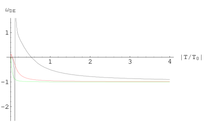
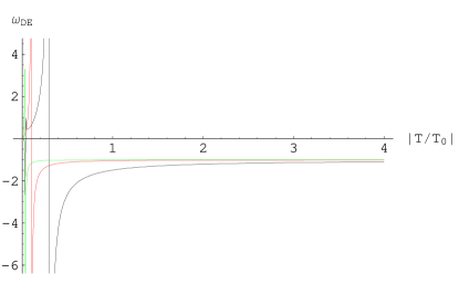
Figure 1: Plot of Ο‰D​Esubscriptπœ”π·πΈ\omega_{DE} versus ∣T/T0∣delimited-βˆ£βˆ£π‘‡subscript𝑇0\mid T/T_{0}\mid with m=2π‘š2m=2 for model I. In left graph, |p|=0.1𝑝0.1|p|=0.1 (black), 0.010.010.01 (red), 0.0010.0010.001 (green) and in right graph |p|=βˆ’0.1𝑝0.1|p|=-0.1 (black), βˆ’0.010.01-0.01 (red), βˆ’0.0010.001-0.001 (green).

The graphical behavior of Ο‰D​Esubscriptπœ”π·πΈ\omega_{DE} as a function of ∣T/T0∣delimited-βˆ£βˆ£π‘‡subscript𝑇0\mid T/T_{0}\mid is shown in Figure 1. For both p>0𝑝0p>0 and p<0,Ο‰D​E𝑝0subscriptπœ”π·πΈp<0,~{}\omega_{DE} reaches to βˆ’11-1 but does not cross the phantom divide line (Ο‰D​E=βˆ’1)subscriptπœ”π·πΈ1(\omega_{DE}=-1). Thus the universe stays in DE era as ∣T/T0∣delimited-βˆ£βˆ£π‘‡subscript𝑇0\mid T/T_{0}\mid approaches to infinity.

Inserting Eq.(17) in (10) and using (26) and (28), we get a torsion scalar as a function of redshift z𝑧z

T=βˆ’2​(2​m+1)​(1+z)6​nm+2,T0=βˆ’2​(2​m+1).formulae-sequence𝑇22π‘š1superscript1𝑧6π‘›π‘š2subscript𝑇022π‘š1T=-2(2m+1)(1+z)^{\frac{6n}{m+2}},\quad T_{0}=-2(2m+1). (30)

Substituting these values in Eq.(29), the corresponding EoS parameter in terms of z𝑧z takes the following form as

Ο‰D​E=βˆ’p​ep​(1+z)βˆ’6​nm+2D​(1+z)6​nm+2​[βˆ’1+2​(4​m+5)​p(2​m+1)​(1+z)6​nm+2],subscriptπœ”π·πΈπ‘superscript𝑒𝑝superscript1𝑧6π‘›π‘š2𝐷superscript1𝑧6π‘›π‘š2delimited-[]124π‘š5𝑝2π‘š1superscript1𝑧6π‘›π‘š2\omega_{DE}=-\frac{pe^{p(1+z)^{\frac{-6n}{m+2}}}}{D(1+z)^{\frac{6n}{m+2}}}\left[-1+\frac{2(4m+5)p}{(2m+1)(1+z)^{\frac{6n}{m+2}}}\right], (31)

where

D𝐷\displaystyle D =\displaystyle= [3​(1βˆ’ep​(1+z)βˆ’6​nm+2)+2​p​(1+z)βˆ’6​nm+2​ep​(1+z)βˆ’6​nm+2]delimited-[]31superscript𝑒𝑝superscript1𝑧6π‘›π‘š22𝑝superscript1𝑧6π‘›π‘š2superscript𝑒𝑝superscript1𝑧6π‘›π‘š2\displaystyle\left[3\left(1-e^{p(1+z)^{\frac{-6n}{m+2}}}\right)+2p(1+z)^{\frac{-6n}{m+2}}e^{p(1+z)^{\frac{-6n}{m+2}}}\right]
Γ—\displaystyle\times [1+Ξ±(1βˆ’ep​(1+z)βˆ’6​nm+2)+Ξ±p(1+z)βˆ’6​nm+2ep​(1+z)βˆ’6​nm+2\displaystyle\left[1+\alpha\left(1-e^{p(1+z)^{\frac{-6n}{m+2}}}\right)+\alpha p(1+z)^{\frac{-6n}{m+2}}e^{p(1+z)^{\frac{-6n}{m+2}}}\right.
Γ—\displaystyle\times (1βˆ’2p(1+z)βˆ’6​nm+2)].\displaystyle\left.\left(1-2p(1+z)^{\frac{-6n}{m+2}}\right)\right].
Refer to caption
Refer to caption
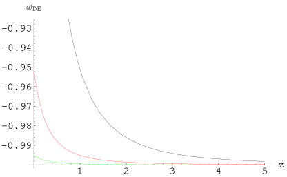
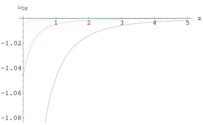
Figure 2: Plot of Ο‰D​Esubscriptπœ”π·πΈ\omega_{DE} versus redshift z𝑧z for model I with m=2,n=2formulae-sequenceπ‘š2𝑛2m=2,~{}n=2 and the same values of the parameter p𝑝p as in Figure 1.

The graphical representation of Ο‰D​Esubscriptπœ”π·πΈ\omega_{DE} versus redshift is shown in Figure 2. We see from the left graph that for p>0,Ο‰D​E𝑝0subscriptπœ”π·πΈp>0,~{}\omega_{DE} increases towards negative and attains βˆ’11-1 but does not cross the phantom divide line for zβ†’βˆžβ†’π‘§z\rightarrow\infty. Thus the universe stays in non-phantom phase (quintessence). For p<0,Ο‰D​E𝑝0subscriptπœ”π·πΈp<0,~{}\omega_{DE} is less than βˆ’11-1 without crossing the phantom divide line and gives the phantom phase of the universe initially. As zβ†’βˆžβ†’π‘§z\rightarrow\infty, it reaches to βˆ’11-1 which is shown in the right graph of Figure 2. Thus the universe always stays in DE era for both cases.
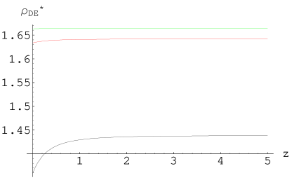
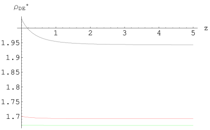
The parameter ρD​E(βˆ—)≑ρD​E/ρD​E(0)superscriptsubscript𝜌𝐷𝐸subscript𝜌𝐷𝐸superscriptsubscript𝜌𝐷𝐸0\rho_{DE}^{(*)}\equiv\rho_{DE}/\rho_{DE}^{(0)} in terms of z𝑧z is obtained by putting Eq.(30) in (23) as

ρD​E(βˆ—)=(2​m+1)​(1+z)6​nm+2​α8​π​G​ρD​E(0)​[3​(1βˆ’ep/(1+z)6​nm+2)+2​p​ep/(1+z)6​nm+2(1+z)6​nm+2],superscriptsubscript𝜌𝐷𝐸2π‘š1superscript1𝑧6π‘›π‘š2𝛼8πœ‹πΊsuperscriptsubscript𝜌𝐷𝐸0delimited-[]31superscript𝑒𝑝superscript1𝑧6π‘›π‘š22𝑝superscript𝑒𝑝superscript1𝑧6π‘›π‘š2superscript1𝑧6π‘›π‘š2\rho_{DE}^{(*)}=\frac{(2m+1)(1+z)^{\frac{6n}{m+2}}\alpha}{8\pi G\rho_{DE}^{(0)}}\left[3\left(1-e^{p/(1+z)^{\frac{6n}{m+2}}}\right)+\frac{2pe^{p/(1+z)^{\frac{6n}{m+2}}}}{(1+z)^{\frac{6n}{m+2}}}\right], (32)

where ρD​E(0)=0.74​ρc​r​i​t(0)superscriptsubscript𝜌𝐷𝐸00.74subscriptsuperscript𝜌0π‘π‘Ÿπ‘–π‘‘\rho_{DE}^{(0)}=0.74~{}\rho^{(0)}_{crit} (Bamba et al. 2011).

Refer to caption
Refer to caption
Figure 3: Plot of ρD​E(βˆ—)superscriptsubscript𝜌𝐷𝐸\rho_{DE}^{(*)} versus z𝑧z keeping same parameters as in Figure 2.

The evolution of ρD​E(βˆ—)superscriptsubscript𝜌𝐷𝐸\rho_{DE}^{(*)} in terms of redshift z𝑧z for p>0𝑝0p>0 and p<0𝑝0p<0 is shown in Figure 3. For p>0𝑝0p>0, this indicates a slight increment in ρD​E(βˆ—)superscriptsubscript𝜌𝐷𝐸\rho_{DE}^{(*)} for smaller values of z𝑧z and becomes constant for larger values of z𝑧z. When p<0𝑝0p<0, it decreases initially with respect to z𝑧z and approaches to constant value as zβ†’βˆžβ†’π‘§z\rightarrow\infty. We would like to mention here that ρD​E(βˆ—)superscriptsubscript𝜌𝐷𝐸\rho_{DE}^{(*)} attains different values at z=0𝑧0z=0 for both the cases of p𝑝p for BI universe. On the other hand, ρD​E(βˆ—)​(z=0)superscriptsubscriptπœŒπ·πΈπ‘§0\rho_{DE}^{(*)}(z=0) coincides at the same point for several values of p𝑝p for FRW universe (Bamba et al. 2011).

Now we discuss the viability of the exponential f​(T)𝑓𝑇f(T) model for phantom and non-phantom phases by using an approximate method. From Eq.(27), we obtain

fT=α​(1βˆ’ep​T0/T+p​T0T​ep​T0/T),fT​T=βˆ’Ξ±β€‹(p​T0T)2​1T​ep​T0/T.formulae-sequencesubscript𝑓𝑇𝛼1superscript𝑒𝑝subscript𝑇0𝑇𝑝subscript𝑇0𝑇superscript𝑒𝑝subscript𝑇0𝑇subscript𝑓𝑇𝑇𝛼superscript𝑝subscript𝑇0𝑇21𝑇superscript𝑒𝑝subscript𝑇0𝑇f_{T}=\alpha\left(1-e^{pT_{0}/T}+\frac{pT_{0}}{T}e^{pT_{0}/T}\right),\quad f_{TT}=-\alpha\left(\frac{pT_{0}}{T}\right)^{2}\frac{1}{T}e^{pT_{0}/T}. (33)

Assuming X=p​T0/T,T0/T≲1formulae-sequence𝑋𝑝subscript𝑇0𝑇less-than-or-similar-tosubscript𝑇0𝑇1X=pT_{0}/T,~{}T_{0}/T\lesssim 1 in Eqs.(27) and (33), it follows that (Bamba et al. 2010b)

fTβ‰ˆβˆ’Ξ±β€‹(X+X22),fTβ‰ˆΞ±β€‹X22,T​fT​Tβ‰ˆβˆ’Ξ±β€‹X2.formulae-sequence𝑓𝑇𝛼𝑋superscript𝑋22formulae-sequencesubscript𝑓𝑇𝛼superscript𝑋22𝑇subscript𝑓𝑇𝑇𝛼superscript𝑋2\frac{f}{T}\approx-\alpha\left(X+\frac{X^{2}}{2}\right),\quad f_{T}\approx\frac{\alpha X^{2}}{2},\quad Tf_{TT}\approx-\alpha X^{2}. (34)

Inserting these values in Eq.(25), Ο‰D​Esubscriptπœ”π·πΈ\omega_{DE} takes the form

Ο‰D​Eβ‰ˆβˆ’1+14​m+192​(2​m+1)​X.subscriptπœ”π·πΈ114π‘š1922π‘š1𝑋\omega_{DE}\approx-1+\frac{14m+19}{2(2m+1)}X. (35)

Here, we have take α∼O​(1)similar-to𝛼𝑂1\alpha\sim O(1). This implies that the behavior of EoS parameter depends on the sign of p𝑝p and correspondingly on X𝑋X. For X>0𝑋0X>0, the universe always stays in non-phantom phase as Ο‰D​E>βˆ’1subscriptπœ”π·πΈ1\omega_{DE}>-1. The universe rests in the phantom region for X<0𝑋0X<0 as Ο‰D​E<βˆ’1subscriptπœ”π·πΈ1\omega_{DE}<-1. This is consistent with the graphical results shown in Figure 2.

4.2 Model II

Assume the logarithmic f​(T)𝑓𝑇f(T) model as (Bamba et al. 2011)

f​(T)=β​T0​(q​T0T)βˆ’1/2​ln⁑(q​T0T),𝑓𝑇𝛽subscript𝑇0superscriptπ‘žsubscript𝑇0𝑇12π‘žsubscript𝑇0𝑇f(T)=\beta T_{0}\left(\frac{qT_{0}}{T}\right)^{-1/2}\ln\left(\frac{qT_{0}}{T}\right), (36)

where

β≑1βˆ’Ξ©M(0)2​qβˆ’1/2,q>0.formulae-sequence𝛽1subscriptsuperscriptΞ©0𝑀2superscriptπ‘ž12π‘ž0\beta\equiv\frac{1-\Omega^{(0)}_{M}}{2q^{-1/2}},\quad q>0.

If the value of Ξ©M(0)subscriptsuperscriptΞ©0𝑀\Omega^{(0)}_{M} is given, then the only parameter qπ‘žq is involved in the logarithmic f​(T)𝑓𝑇f(T) model same as the exponential f​(T)𝑓𝑇f(T) model. The corresponding EoS parameter is given by

Ο‰D​E=βˆ’[1+3​(m+1)2​m+1​ln⁑(T0/T)][2βˆ’(1βˆ’Ξ©M(0))​(T0/T)1/2]​[ln⁑(T0/T)βˆ’1]subscriptπœ”π·πΈdelimited-[]13π‘š12π‘š1subscript𝑇0𝑇delimited-[]21subscriptsuperscriptΞ©0𝑀superscriptsubscript𝑇0𝑇12delimited-[]subscript𝑇0𝑇1\omega_{DE}=-\frac{[1+\frac{3(m+1)}{2m+1}\ln(T_{0}/T)]}{[2-(1-\Omega^{(0)}_{M})(T_{0}/T)^{1/2}][\ln(T_{0}/T)-1]} (37)

which is independent of qπ‘žq. Using Eq.(30) in above equation, Ο‰D​Esubscriptπœ”π·πΈ\omega_{DE} in terms of redshift z𝑧z becomes

Ο‰D​E=βˆ’[1+3​(m+1)2​m+1​ln⁑(1/(1+z)6​nm+2)][2βˆ’(1βˆ’Ξ©M(0))​(1/(1+z)6​nm+2)1/2]​[ln⁑(1/(1+z)6​nm+2)βˆ’1].subscriptπœ”π·πΈdelimited-[]13π‘š12π‘š11superscript1𝑧6π‘›π‘š2delimited-[]21subscriptsuperscriptΞ©0𝑀superscript1superscript1𝑧6π‘›π‘š212delimited-[]1superscript1𝑧6π‘›π‘š21\omega_{DE}=-\frac{[1+\frac{3(m+1)}{2m+1}\ln(1/(1+z)^{\frac{6n}{m+2}})]}{[2-(1-\Omega^{(0)}_{M})(1/(1+z)^{\frac{6n}{m+2}})^{1/2}][\ln(1/(1+z)^{\frac{6n}{m+2}})-1]}. (38)
Refer to caption
Refer to caption
Figure 4: Plot of Ο‰D​Esubscriptπœ”π·πΈ\omega_{DE} versus ∣T/T0∣delimited-βˆ£βˆ£π‘‡subscript𝑇0\mid T/T_{0}\mid in left side and Ο‰D​Esubscriptπœ”π·πΈ\omega_{DE} versus z𝑧z in right side for q=1,m=2=nformulae-sequenceπ‘ž1π‘š2𝑛q=1,~{}m=2=n and Ξ©M(0)=0.26subscriptsuperscriptΞ©0𝑀0.26\Omega^{(0)}_{M}=0.26 for model II.

Its behavior is shown in Figure 4. The left graph shows that Ο‰D​Esubscriptπœ”π·πΈ\omega_{DE} becomes negative as ∣T/T0βˆ£β†’βˆžβ†’delimited-βˆ£βˆ£π‘‡subscript𝑇0\mid T/T_{0}\mid\rightarrow\infty. In the beginning, the model represents a universe having both properties of matter and radiation. After a very short interval, the universe enters in DE phase. It is mentioned here that the universe remains in non-phantom phase as the time elapses. The right graph has the same behavior as that of the exponential f​(T)𝑓𝑇f(T) model and the universe stays in the non-phantom phase (Ο‰D​E>βˆ’1subscriptπœ”π·πΈ1\omega_{DE}>-1).

4.3 Model III

Here we take the combination of both exponential and logarithmic f​(T)𝑓𝑇f(T) models which has the following form (Bamba et al. 2011)

f​(T)=γ​[T0​(u​T0T)βˆ’1/2​ln⁑(u​T0T)βˆ’T​(1βˆ’eu​T0/T)],𝑓𝑇𝛾delimited-[]subscript𝑇0superscript𝑒subscript𝑇0𝑇12𝑒subscript𝑇0𝑇𝑇1superscript𝑒𝑒subscript𝑇0𝑇f(T)=\gamma\left[T_{0}\left(\frac{uT_{0}}{T}\right)^{-1/2}\ln\left(\frac{uT_{0}}{T}\right)-T(1-e^{uT_{0}/T})\right], (39)

where

γ≑1βˆ’Ξ©M(0)2​uβˆ’1/2+[1βˆ’(1βˆ’2​u)​eu].𝛾1subscriptsuperscriptΞ©0𝑀2superscript𝑒12delimited-[]112𝑒superscript𝑒𝑒\gamma\equiv\frac{1-\Omega^{(0)}_{M}}{2u^{-1/2}+[1-(1-2u)e^{u}]}.

The positive constant u𝑒u is the only parameter in this model. The EoS parameter for DE in terms of ∣T/T0∣delimited-βˆ£βˆ£π‘‡subscript𝑇0\mid T/T_{0}\mid is given by

Ο‰D​Esubscriptπœ”π·πΈ\displaystyle\omega_{DE} =\displaystyle= βˆ’1I[1uu​T0T{1+3​(m+1)2​m+1ln(u​T0T)}\displaystyle-\frac{1}{I}\left[\frac{1}{u}\sqrt{\frac{uT_{0}}{T}}\left\{1+\frac{3(m+1)}{2m+1}\ln\left(\frac{uT_{0}}{T}\right)\right\}\right. (40)
+\displaystyle+ eu​T0/T(u​T0T){1βˆ’2​(4​m+5)2​m+1(u​T0T)}],\displaystyle\left.e^{uT_{0}/T}\left(\frac{uT_{0}}{T}\right)\left\{1-\frac{2(4m+5)}{2m+1}\left(\frac{uT_{0}}{T}\right)\right\}\right],

where

I𝐼\displaystyle I =\displaystyle= [2u​u​T0T​{ln⁑(u​T0T)βˆ’1}+eu​T0/T​(3βˆ’2​u​T0T)βˆ’3]delimited-[]2𝑒𝑒subscript𝑇0𝑇𝑒subscript𝑇0𝑇1superscript𝑒𝑒subscript𝑇0𝑇32𝑒subscript𝑇0𝑇3\displaystyle\left[\frac{2}{u}\sqrt{\frac{uT_{0}}{T}}\left\{\ln\left(\frac{uT_{0}}{T}\right)-1\right\}+e^{uT_{0}/T}\left(3-\frac{2uT_{0}}{T}\right)-3\right]
Γ—\displaystyle\times [1βˆ’Ξ³β€‹(1βˆ’eu​T0/T)βˆ’Ξ³β€‹u​T0T​{1u+u​T0T​eu​T0/T​(1βˆ’2​u​T0T)}].delimited-[]1𝛾1superscript𝑒𝑒subscript𝑇0𝑇𝛾𝑒subscript𝑇0𝑇1𝑒𝑒subscript𝑇0𝑇superscript𝑒𝑒subscript𝑇0𝑇12𝑒subscript𝑇0𝑇\displaystyle\left[1-\gamma(1-e^{uT_{0}/T})-\gamma\sqrt{\frac{uT_{0}}{T}}\left\{\frac{1}{u}+\sqrt{\frac{uT_{0}}{T}}e^{uT_{0}/T}\left(1-\frac{2uT_{0}}{T}\right)\right\}\right].
Refer to caption
Refer to caption
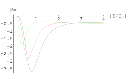
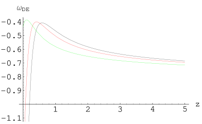
Figure 5: Plot of Ο‰D​Esubscriptπœ”π·πΈ\omega_{DE} versus ∣T/T0∣delimited-βˆ£βˆ£π‘‡subscript𝑇0\mid T/T_{0}\mid in left graph and Ο‰D​Esubscriptπœ”π·πΈ\omega_{DE} versus z𝑧z in right graph with m=2=nπ‘š2𝑛m=2=n and u=1𝑒1u=1 (black line), 0.80.80.8 (red line), 0.50.50.5 (green) for model III.

Initially, the expanding universe is lying in non-phantom phase with Ο‰D​Esubscriptπœ”π·πΈ\omega_{DE} as a function of ∣T/T0∣delimited-βˆ£βˆ£π‘‡subscript𝑇0\mid T/T_{0}\mid as shown in left graph of Figure 5. The EoS parameter decreases with increase in ∣T/T0∣delimited-βˆ£βˆ£π‘‡subscript𝑇0\mid T/T_{0}\mid by crossing the phantom divide line at ∣T/T0∣=0.27,0.36delimited-βˆ£βˆ£π‘‡subscript𝑇00.270.36\mid T/T_{0}\mid=0.27,~{}0.36 and 0.420.420.42 for u=0.5,0.8𝑒0.50.8u=0.5,~{}0.8 and 111 respectively evolving the phantom phase. After a short interval, Ο‰D​Esubscriptπœ”π·πΈ\omega_{DE} crosses the phantom divide line again at ∣T/T0∣=0.65,1.2delimited-βˆ£βˆ£π‘‡subscript𝑇00.651.2\mid T/T_{0}\mid=0.65,~{}1.2 and 1.71.71.7 which turns out to be constant as ∣T/T0∣delimited-βˆ£βˆ£π‘‡subscript𝑇0\mid T/T_{0}\mid increases.

Inserting Eq.(30) in (40), Ο‰D​Esubscriptπœ”π·πΈ\omega_{DE} in terms of z𝑧z turns to be

Ο‰D​Esubscriptπœ”π·πΈ\displaystyle\omega_{DE} =\displaystyle= βˆ’1F[1uu​(1+z)βˆ’6​nm+2{1+3​(m+1)2​m+1ln(u(1+z)βˆ’6​nm+2)}\displaystyle-\frac{1}{F}\left[\frac{1}{u}{\sqrt{u(1+z)^{\frac{-6n}{m+2}}}}\left\{1+\frac{3(m+1)}{2m+1}\ln\left(u(1+z)^{\frac{-6n}{m+2}}\right)\right\}\right. (41)
+\displaystyle+ u(1+z)βˆ’6​nm+2eu​(1+z)βˆ’6​nm+2(1βˆ’2​u​(4​m+5)​(1+z)βˆ’6​nm+2(2​m+1))],\displaystyle\left.u(1+z)^{\frac{-6n}{m+2}}e^{u(1+z)^{\frac{-6n}{m+2}}}\left(1-\frac{2u(4m+5)(1+z)^{\frac{-6n}{m+2}}}{(2m+1)}\right)\right],

where

F𝐹\displaystyle F =\displaystyle= [2uu​(1+z)βˆ’6​nm+2(ln(u(1+z)βˆ’6​nm+2)βˆ’1)+eu​(1+z)βˆ’6​nm+2\displaystyle\left[\frac{2}{u}{\sqrt{u(1+z)^{\frac{-6n}{m+2}}}}\left(\ln\left(u(1+z)^{\frac{-6n}{m+2}}\right)-1\right)+e^{u(1+z)^{\frac{-6n}{m+2}}}\right.
Γ—\displaystyle\times {3βˆ’2u(1+z)βˆ’6​nm+2}βˆ’3][1βˆ’Ξ³(1βˆ’eu​(1+z)βˆ’6​nm+2)βˆ’Ξ³u​(1+z)βˆ’6​nm+2\displaystyle\left.\left\{3-2u(1+z)^{\frac{-6n}{m+2}}\right\}-3\right]\left[1-\gamma\left(1-e^{u(1+z)^{\frac{-6n}{m+2}}}\right)-\gamma{\sqrt{u(1+z)^{\frac{-6n}{m+2}}}}\right.
Γ—\displaystyle\times {1u+eu​(1+z)βˆ’6​nm+2(1βˆ’2u(1+z)βˆ’6​nm+2)u​(1+z)βˆ’6​nm+2}].\displaystyle\left.\left\{\frac{1}{u}+e^{u(1+z)^{\frac{-6n}{m+2}}}\left(1-2u(1+z)^{\frac{-6n}{m+2}}\right){\sqrt{u(1+z)^{\frac{-6n}{m+2}}}}\right\}\right].

The right graph of Figure 5 shows that for u=0.8𝑒0.8u=0.8 and u=1𝑒1u=1, the universe is in the phantom phase (Ο‰D​E<βˆ’1subscriptπœ”π·πΈ1\omega_{DE}<-1) at initial epoch. As z𝑧z increases, it crosses the phantom divide line (Ο‰D​E=βˆ’1subscriptπœ”π·πΈ1\omega_{DE}=-1) at z=0.067𝑧0.067z=0.067 and 0.180.180.18 respectively. Thus Ο‰D​Esubscriptπœ”π·πΈ\omega_{DE} enters in the non-phantom phase and converges to constant value with increment in z𝑧z. It is interesting to note that for u≀0.6𝑒0.6u\leq 0.6, the universe always rests in non-phantom phase. Notice that the combined f​(T)𝑓𝑇f(T) model behaves as the quintom model (Khatua et al. 2011).

4.4 Model IV

Now we take the f​(T)𝑓𝑇f(T) model of the type (Yang 2011)

f​(T)=T+η​T0​(T2/T02)Ξ»1+(T2/T02)Ξ»,π‘“π‘‡π‘‡πœ‚subscript𝑇0superscriptsuperscript𝑇2superscriptsubscript𝑇02πœ†1superscriptsuperscript𝑇2superscriptsubscript𝑇02πœ†f(T)=T+\eta T_{0}\frac{(T^{2}/T_{0}^{2})^{\lambda}}{1+(T^{2}/T_{0}^{2})^{\lambda}}, (42)

where Ξ·πœ‚\eta and Ξ»πœ†\lambda are positive constants. The corresponding EoS parameter is

Ο‰D​Esubscriptπœ”π·πΈ\displaystyle\omega_{DE} =\displaystyle= βˆ’Ξ·β€‹(T/T0)2β€‹Ξ»βˆ’1K​(1+(T2/T02)Ξ»)[1βˆ’2Ξ»{1βˆ’(T2/T02)Ξ»(1+(T2/T02)Ξ»)\displaystyle-\frac{\eta(T/T_{0})^{2\lambda-1}}{K(1+(T^{2}/T_{0}^{2})^{\lambda})}\left[1-2\lambda\left\{1-\frac{(T^{2}/T_{0}^{2})^{\lambda}}{(1+(T^{2}/T_{0}^{2})^{\lambda})}\right.\right. (43)
+\displaystyle+ (2β€‹Ξ»βˆ’1βˆ’(T2/T02)Ξ»1+(T2/T02)λ​(6β€‹Ξ»βˆ’1βˆ’4​λ​(T2/T02)Ξ»1+(T2/T02)Ξ»))2πœ†1superscriptsuperscript𝑇2superscriptsubscript𝑇02πœ†1superscriptsuperscript𝑇2superscriptsubscript𝑇02πœ†6πœ†14πœ†superscriptsuperscript𝑇2superscriptsubscript𝑇02πœ†1superscriptsuperscript𝑇2superscriptsubscript𝑇02πœ†\displaystyle\left.\left.\left(2\lambda-1-\frac{(T^{2}/T_{0}^{2})^{\lambda}}{1+(T^{2}/T_{0}^{2})^{\lambda}}\left(6\lambda-1-\frac{4\lambda(T^{2}/T_{0}^{2})^{\lambda}}{1+(T^{2}/T_{0}^{2})^{\lambda}}\right)\right)\right.\right.
Γ—\displaystyle\times 2​(4​m+5)2​m+1}],\displaystyle\left.\left.\frac{2(4m+5)}{2m+1}\right\}\right],

where

K𝐾\displaystyle K =\displaystyle= [3+η​(T/T0)2β€‹Ξ»βˆ’11+(T2/T02)λ​{1+4​λ​(1βˆ’(T2/T02)Ξ»1+(T2/T02)Ξ»)}]delimited-[]3πœ‚superscript𝑇subscript𝑇02πœ†11superscriptsuperscript𝑇2superscriptsubscript𝑇02πœ†14πœ†1superscriptsuperscript𝑇2superscriptsubscript𝑇02πœ†1superscriptsuperscript𝑇2superscriptsubscript𝑇02πœ†\displaystyle\left[3+\frac{\eta(T/T_{0})^{2\lambda-1}}{1+(T^{2}/T_{0}^{2})^{\lambda}}\left\{1+4\lambda\left(1-\frac{(T^{2}/T_{0}^{2})^{\lambda}}{1+(T^{2}/T_{0}^{2})^{\lambda}}\right)\right\}\right]
Γ—\displaystyle\times [1+2​η​λ​(T/T0)2β€‹Ξ»βˆ’11+(T2/T02)Ξ»{4Ξ»βˆ’1+(T2/T02)Ξ»1+(T2/T02)Ξ»\displaystyle\left[1+\frac{2\eta\lambda(T/T_{0})^{2\lambda-1}}{1+(T^{2}/T_{0}^{2})^{\lambda}}\left\{4\lambda-1+\frac{(T^{2}/T_{0}^{2})^{\lambda}}{1+(T^{2}/T_{0}^{2})^{\lambda}}\right.\right.
Γ—\displaystyle\times (12Ξ»βˆ’1+8​λ​(T2/T02)Ξ»1+(T2/T02)Ξ»)}].\displaystyle\left.\left.\left(12\lambda-1+\frac{8\lambda(T^{2}/T_{0}^{2})^{\lambda}}{1+(T^{2}/T_{0}^{2})^{\lambda}}\right)\right\}\right].
Refer to caption
Refer to caption
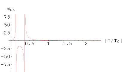
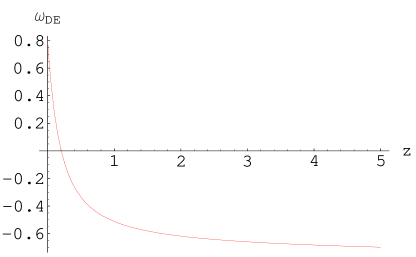
Figure 6: Plot of Ο‰D​Esubscriptπœ”π·πΈ\omega_{DE} versus ∣T/T0∣delimited-βˆ£βˆ£π‘‡subscript𝑇0\mid T/T_{0}\mid and Ο‰D​Esubscriptπœ”π·πΈ\omega_{DE} versus z𝑧z for m=2=n,Ξ·=3formulae-sequenceπ‘š2π‘›πœ‚3m=2=n,~{}\eta=3 and Ξ»=2πœ†2\lambda=2 for model IV.

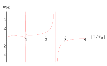
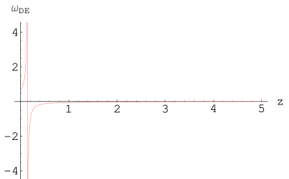
The left graph of Ο‰D​Esubscriptπœ”π·πΈ\omega_{DE} as a function of ∣T/T0∣delimited-βˆ£βˆ£π‘‡subscript𝑇0\mid T/T_{0}\mid is shown in Figure 6. Initially, the behavior of Ο‰D​Esubscriptπœ”π·πΈ\omega_{DE} is positive and stays in radiation era for very small region. After a slight variation in ∣T/T0∣delimited-βˆ£βˆ£π‘‡subscript𝑇0\mid T/T_{0}\mid, the crossing of phantom divide line occurs and results a phantom era. There are two singularities at ∣T/T0∣=0.95delimited-βˆ£βˆ£π‘‡subscript𝑇00.95\mid T/T_{0}\mid=0.95 and 2.52.52.5 with positive behavior. After these singularities, Ο‰D​Esubscriptπœ”π·πΈ\omega_{DE} evolves from phantom to non-phantom phase by crossing phantom divide line and remains in non-phantom phase for ∣T/T0βˆ£β†’βˆžβ†’delimited-βˆ£βˆ£π‘‡subscript𝑇0\mid T/T_{0}\mid\rightarrow\infty causing accelerated expansion of the universe. In term of z𝑧z, the parameter Ο‰D​Esubscriptπœ”π·πΈ\omega_{DE} is obtained by using Eq.(30) in (43) as

Ο‰D​Esubscriptπœ”π·πΈ\displaystyle\omega_{DE} =\displaystyle= βˆ’Ξ·β€‹(1+z)6​n​(2β€‹Ξ»βˆ’1)m+2J​(1+(1+z)12​n​λm+2)[1βˆ’2Ξ»{1βˆ’(1+z)12​n​λm+21+(1+z)12​n​λm+2+2​(4​m+5)2​m+1\displaystyle-\frac{\eta(1+z)^{\frac{6n(2\lambda-1)}{m+2}}}{J(1+(1+z)^{\frac{12n\lambda}{m+2}})}\left[1-2\lambda\left\{1-\frac{(1+z)^{\frac{12n\lambda}{m+2}}}{1+(1+z)^{\frac{12n\lambda}{m+2}}}+\frac{2(4m+5)}{2m+1}\right.\right.
Γ—\displaystyle\times (2Ξ»βˆ’1βˆ’(1+z)12​n​λm+21+(1+z)12​n​λm+2(6Ξ»βˆ’1βˆ’4Ξ»(1+z)12​n​λm+21+(1+z)12​n​λm+2))}],\displaystyle\left.\left.\left(2\lambda-1-\frac{(1+z)^{\frac{12n\lambda}{m+2}}}{1+(1+z)^{\frac{12n\lambda}{m+2}}}\left(6\lambda-1-4\lambda\frac{(1+z)^{\frac{12n\lambda}{m+2}}}{1+(1+z)^{\frac{12n\lambda}{m+2}}}\right)\right)\right\}\right],

where

J𝐽\displaystyle J =\displaystyle= [3+η​(1+z)6​n​(2β€‹Ξ»βˆ’1)m+21+(1+z)12​n​λm+2​{1+4​λ​(1βˆ’(1+z)12​n​λm+21+(1+z)12​n​λm+2)}]delimited-[]3πœ‚superscript1𝑧6𝑛2πœ†1π‘š21superscript1𝑧12π‘›πœ†π‘š214πœ†1superscript1𝑧12π‘›πœ†π‘š21superscript1𝑧12π‘›πœ†π‘š2\displaystyle\left[3+\frac{\eta(1+z)^{\frac{6n(2\lambda-1)}{m+2}}}{1+(1+z)^{\frac{12n\lambda}{m+2}}}\left\{1+4\lambda\left(1-\frac{(1+z)^{\frac{12n\lambda}{m+2}}}{1+(1+z)^{\frac{12n\lambda}{m+2}}}\right)\right\}\right]
Γ—\displaystyle\times [1+2​η​λ​(1+z)6​n​(2β€‹Ξ»βˆ’1)m+21+(1+z)12​n​λm+2{4Ξ»βˆ’1+(1+z)12​n​λm+21+(1+z)12​n​λm+2\displaystyle\left[1+\frac{2\eta\lambda(1+z)^{\frac{6n(2\lambda-1)}{m+2}}}{1+(1+z)^{\frac{12n\lambda}{m+2}}}\left\{4\lambda-1+\frac{(1+z)^{\frac{12n\lambda}{m+2}}}{1+(1+z)^{\frac{12n\lambda}{m+2}}}\right.\right.
Γ—\displaystyle\times (12Ξ»βˆ’1+8​λ​(1+z)12​n​λm+21+(1+z)12​n​λm+2)}].\displaystyle\left.\left.\left(12\lambda-1+\frac{8\lambda(1+z)^{\frac{12n\lambda}{m+2}}}{1+(1+z)^{\frac{12n\lambda}{m+2}}}\right)\right\}\right].

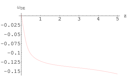
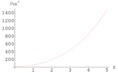
For small values of z𝑧z, Ο‰D​Esubscriptπœ”π·πΈ\omega_{DE} is found to be the non-phantom phase and converges to zero with the increment in the value of z𝑧z. This shows that matter becomes dominant over the DE as shown in right side of Figure 6. Inserting Eq.(30) in (23), the corresponding parameter ρD​E(βˆ—)​(z)superscriptsubscriptπœŒπ·πΈπ‘§\rho_{DE}^{(*)}(z) can be written as

ρD​E(βˆ—)superscriptsubscript𝜌𝐷𝐸\displaystyle\rho_{DE}^{(*)} =\displaystyle= (2​m+1)​(1+z)6​nm+28​π​G​ρD​E(0)[3+η​(1+z)6​n​(2β€‹Ξ»βˆ’1)m+21+(1+z)12​n​λm+2\displaystyle\frac{(2m+1)(1+z)^{\frac{6n}{m+2}}}{8\pi G\rho_{DE}^{(0)}}\left[3+\frac{\eta(1+z)^{\frac{6n(2\lambda-1)}{m+2}}}{1+(1+z)^{\frac{12n\lambda}{m+2}}}\right. (45)
Γ—\displaystyle\times {1+4Ξ»(1βˆ’(1+z)12​n​λm+21+(1+z)12​n​λm+2)}].\displaystyle\left.\left\{1+4\lambda\left(1-\frac{(1+z)^{\frac{12n\lambda}{m+2}}}{1+(1+z)^{\frac{12n\lambda}{m+2}}}\right)\right\}\right].
Refer to caption
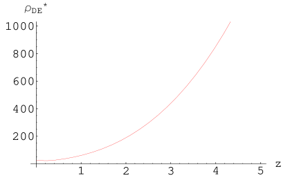
Figure 7: Plot of ρD​E(βˆ—)superscriptsubscript𝜌𝐷𝐸\rho_{DE}^{(*)} versus z𝑧z with same values of parameters as in Figure 6.

The graphical representation (Figure 7) shows the increasing behavior of ρD​E(βˆ—)superscriptsubscript𝜌𝐷𝐸\rho_{DE}^{(*)} for zβ†’βˆžβ†’π‘§z\rightarrow\infty.

4.5 Model V

Finally, we take the f​(T)𝑓𝑇f(T) model in the form (Yang 2011)

f​(T)=Tβˆ’Ξ·β€‹T0​[(1+T2T02)βˆ’Ξ»βˆ’1].π‘“π‘‡π‘‡πœ‚subscript𝑇0delimited-[]superscript1superscript𝑇2superscriptsubscript𝑇02πœ†1f(T)=T-\eta T_{0}\left[\left(1+\frac{T^{2}}{T_{0}^{2}}\right)^{-\lambda}-1\right]. (46)

The expression for Ο‰D​Esubscriptπœ”π·πΈ\omega_{DE} takes the form

Ο‰D​Esubscriptπœ”π·πΈ\displaystyle\omega_{DE} =\displaystyle= 1L[Ξ·(TT0){1βˆ’(1+T2T02)βˆ’Ξ»}βˆ’2Ξ·Ξ»(TT0)(1+T2T02)βˆ’Ξ»βˆ’1\displaystyle\frac{1}{L}\left[\eta\left(\frac{T}{T_{0}}\right)\left\{1-\left(1+\frac{T^{2}}{T^{2}_{0}}\right)^{-\lambda}\right\}-2\eta\lambda\left(\frac{T}{T_{0}}\right)\left(1+\frac{T^{2}}{T^{2}_{0}}\right)^{-\lambda-1}\right. (47)
Γ—\displaystyle\times {1+2​(4​m+5)2​m+1(1βˆ’2(Ξ»+1)(TT0)2(1+T2T02)βˆ’1)}],\displaystyle\left.\left\{1+\frac{2(4m+5)}{2m+1}\left(1-2(\lambda+1)\left(\frac{T}{T_{0}}\right)^{2}\left(1+\frac{T^{2}}{T^{2}_{0}}\right)^{-1}\right)\right\}\right],

where

L𝐿\displaystyle L =\displaystyle= [2+2​η​λ​(TT0)​(1+T2T02)βˆ’Ξ»βˆ’1​{3βˆ’4​(Ξ»+1)​(TT0)2​(1+T2T02)βˆ’1}]delimited-[]22πœ‚πœ†π‘‡subscript𝑇0superscript1superscript𝑇2subscriptsuperscript𝑇20πœ†134πœ†1superscript𝑇subscript𝑇02superscript1superscript𝑇2subscriptsuperscript𝑇201\displaystyle\left[2+2\eta\lambda\left(\frac{T}{T_{0}}\right)\left(1+\frac{T^{2}}{T^{2}_{0}}\right)^{-\lambda-1}\left\{3-4(\lambda+1)\left(\frac{T}{T_{0}}\right)^{2}\left(1+\frac{T^{2}}{T^{2}_{0}}\right)^{-1}\right\}\right]
Γ—\displaystyle\times [3βˆ’Ξ·β€‹(T0T)​(1+T2T02)βˆ’Ξ»β€‹{1βˆ’4​λ​(TT0)2​(1+T2T02)βˆ’1}+η​(T0T)].delimited-[]3πœ‚subscript𝑇0𝑇superscript1superscript𝑇2subscriptsuperscript𝑇20πœ†14πœ†superscript𝑇subscript𝑇02superscript1superscript𝑇2subscriptsuperscript𝑇201πœ‚subscript𝑇0𝑇\displaystyle\left[3-\eta\left(\frac{T_{0}}{T}\right)\left(1+\frac{T^{2}}{T^{2}_{0}}\right)^{-\lambda}\left\{1-4\lambda\left(\frac{T}{T_{0}}\right)^{2}\left(1+\frac{T^{2}}{T^{2}_{0}}\right)^{-1}\right\}+\eta\left(\frac{T_{0}}{T}\right)\right].

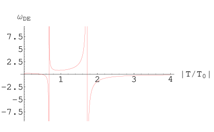
The left graph of Figure 8 represents the cosmological evolution of Ο‰D​Esubscriptπœ”π·πΈ\omega_{DE} in terms of ∣T/T0∣delimited-βˆ£βˆ£π‘‡subscript𝑇0\mid T/T_{0}\mid which shows the same behavior as model IV. However, the singularities appear at ∣T/T0∣=0.7,1.7delimited-βˆ£βˆ£π‘‡subscript𝑇00.71.7\mid T/T_{0}\mid=0.7,~{}1.7 and the universe stays in non-phantom phase for a short interval. Here the universe becomes matter dominated for higher values of ∣T/T0∣delimited-βˆ£βˆ£π‘‡subscript𝑇0\mid T/T_{0}\mid.

Substituting Eq.(30) in (47), the corresponding Ο‰D​Esubscriptπœ”π·πΈ\omega_{DE} as a function of z𝑧z turns out to be

Ο‰D​Esubscriptπœ”π·πΈ\displaystyle\omega_{DE} =\displaystyle= 1M[βˆ’2Ξ·Ξ»(1+z)6​nm+2(1+(1+z)12​nm+2)βˆ’Ξ»βˆ’1\displaystyle\frac{1}{M}\left[-2\eta\lambda(1+z)^{\frac{6n}{m+2}}\left(1+(1+z)^{\frac{12n}{m+2}}\right)^{-\lambda-1}\right. (48)
Γ—\displaystyle\times {1+2​(4​m+5)2​m+1​(1βˆ’2​(Ξ»+1)​(1+z)12​nm+2​(1+(1+z)12​nm+2)βˆ’1)}124π‘š52π‘š112πœ†1superscript1𝑧12π‘›π‘š2superscript1superscript1𝑧12π‘›π‘š21\displaystyle\left.\left\{1+\frac{2(4m+5)}{2m+1}\left(1-2(\lambda+1)(1+z)^{\frac{12n}{m+2}}\left(1+(1+z)^{\frac{12n}{m+2}}\right)^{-1}\right)\right\}\right.
+\displaystyle+ Ξ·((1+z)6​nm+2){1βˆ’(1+(1+z)12​nm+2)βˆ’Ξ»}],\displaystyle\left.\eta\left((1+z)^{\frac{6n}{m+2}}\right)\left\{1-\left(1+(1+z)^{\frac{12n}{m+2}}\right)^{-\lambda}\right\}\right],

where

M𝑀\displaystyle M =\displaystyle= [1+Ξ·Ξ»(1+z)6​nm+2(1+(1+z)12​nm+2)βˆ’Ξ»βˆ’1\displaystyle\left[1+\eta\lambda(1+z)^{\frac{6n}{m+2}}\left(1+(1+z)^{\frac{12n}{m+2}}\right)^{-\lambda-1}\right.
Γ—\displaystyle\times {3βˆ’4(Ξ»+1)(1+z)12​nm+2(1+(1+z)12​nm+2)βˆ’1}]\displaystyle\left.\left\{3-4(\lambda+1)(1+z)^{\frac{12n}{m+2}}\left(1+(1+z)^{\frac{12n}{m+2}}\right)^{-1}\right\}\right]
Γ—\displaystyle\times [3βˆ’Ξ·(1+z)6​nm+2(1+(1+z)12​nm+2)βˆ’Ξ»\displaystyle\left[3-\frac{\eta}{(1+z)^{\frac{6n}{m+2}}}\left(1+(1+z)^{\frac{12n}{m+2}}\right)^{-\lambda}\right.
Γ—\displaystyle\times {1βˆ’4Ξ»(1+z)12​nm+2(1+(1+z)12​nm+2)βˆ’1}+Ξ·(1+z)6​nm+2].\displaystyle\left.\left\{1-4\lambda(1+z)^{\frac{12n}{m+2}}\left(1+(1+z)^{\frac{12n}{m+2}}\right)^{-1}\right\}+\frac{\eta}{(1+z)^{\frac{6n}{m+2}}}\right].
Refer to caption
Refer to caption
Figure 8: Plot of Ο‰D​Esubscriptπœ”π·πΈ\omega_{DE} versus ∣T/T0∣delimited-βˆ£βˆ£π‘‡subscript𝑇0\mid T/T_{0}\mid in the left and Ο‰D​Esubscriptπœ”π·πΈ\omega_{DE} versus z𝑧z in the right for Ξ·=3,Ξ»=3formulae-sequenceπœ‚3πœ†3\eta=3,~{}\lambda=3 and m=2=nπ‘š2𝑛m=2=n for model V.

The parameter Ο‰D​Esubscriptπœ”π·πΈ\omega_{DE} in terms of z𝑧z enters from phantom phase to non-phantom phase and approaches to matter dominated era similar to Ο‰D​E​(T/T0)subscriptπœ”π·πΈπ‘‡subscript𝑇0\omega_{DE}(T/T_{0}) shown in the right graph of Figure 8. Using Eq.(30) in (23), it follows that

ρD​E(βˆ—)​(z)superscriptsubscriptπœŒπ·πΈπ‘§\displaystyle\rho_{DE}^{(*)}(z) =\displaystyle= (2​m+1)​(1+z)6​nm+28​π​G​ρD​E(0)[3βˆ’Ξ·(1+z)6​nm+2(1+(1+z)12​nm+2)βˆ’Ξ»\displaystyle\frac{(2m+1)(1+z)^{\frac{6n}{m+2}}}{8\pi G\rho_{DE}^{(0)}}\left[3-\frac{\eta}{(1+z)^{\frac{6n}{m+2}}}\left(1+(1+z)^{\frac{12n}{m+2}}\right)^{-\lambda}\right. (49)
Γ—\displaystyle\times {1βˆ’4Ξ»(1+z)12​nm+2(1+(1+z)12​nm+2)βˆ’1}+Ξ·(1+z)6​nm+2].\displaystyle\left.\left\{1-4\lambda(1+z)^{\frac{12n}{m+2}}\left(1+(1+z)^{\frac{12n}{m+2}}\right)^{-1}\right\}+\frac{\eta}{(1+z)^{\frac{6n}{m+2}}}\right].
Refer to caption
Figure 9: Plot of ρD​E(βˆ—)superscriptsubscript𝜌𝐷𝐸\rho_{DE}^{(*)} versus z𝑧z for Ξ·=3πœ‚3\eta=3 and Ξ»=2πœ†2\lambda=2

Figure 9 shows that ρD​E(βˆ—)superscriptsubscript𝜌𝐷𝐸\rho_{DE}^{(*)} is positive and increases with zβ†’βˆžβ†’π‘§z\rightarrow\infty.

5 Summary and Conclusion

The main purpose of this paper is to discuss the well-known phenomenon of the universe expansion in the context of f​(T)𝑓𝑇f(T) gravity for BI universe model. We have investigated the cosmological evolution of EoS parameter Ο‰D​Esubscriptπœ”π·πΈ\omega_{DE} and energy density ρD​E(βˆ—)superscriptsubscript𝜌𝐷𝐸\rho_{DE}^{(*)} for some well-known f​(T)𝑓𝑇f(T) models. These parameters are evaluated in terms of ∣T/T0∣delimited-βˆ£βˆ£π‘‡subscript𝑇0\mid T/T_{0}\mid and redshift z𝑧z. The graphical representation of the phantom and non-phantom phases of the expanding universe is examined. The behavior of these models can be summarized as follows:

  • β€’

    Model I is the exponential f​(T)𝑓𝑇f(T) model in which the phase of the universe changes with the sign of parameter p𝑝p. For p>0,Ο‰D​E​(z)𝑝0subscriptπœ”π·πΈπ‘§p>0,~{}\omega_{DE}(z) indicates a universe dominated by the non-phantom era while the phantom phase is obtained for p<0𝑝0p<0. The EoS parameter Ο‰D​E​(∣T/T0∣)subscriptπœ”π·πΈdelimited-βˆ£βˆ£π‘‡subscript𝑇0\omega_{DE}(\mid T/T_{0}\mid) corresponds to the DE phase. The energy density shows positive behavior both for p>0𝑝0p>0 and p<0𝑝0p<0.

  • β€’

    For the logarithmic model II, Ο‰D​Esubscriptπœ”π·πΈ\omega_{DE} as a function of ∣T/T0∣delimited-βˆ£βˆ£π‘‡subscript𝑇0\mid T/T_{0}\mid and z𝑧z remains in non-phantom phase which shows the accelerated expansion of the universe.

  • β€’

    In the combined model III, Ο‰D​E​(∣T/T0∣)subscriptπœ”π·πΈdelimited-βˆ£βˆ£π‘‡subscript𝑇0\omega_{DE}(\mid T/T_{0}\mid) shows that the universe initially transits from the non-phantom to phantom phase. After that, the universe again crosses the phantom divide line and retains its initial phase. On the other hand, Ο‰D​E​(z)subscriptπœ”π·πΈπ‘§\omega_{DE}(z) crosses the phantom divide line from phantom phase to non-phantom phase only once.

  • β€’

    For model IV, the parameter Ο‰D​E​(∣T/T0∣)subscriptπœ”π·πΈdelimited-βˆ£βˆ£π‘‡subscript𝑇0\omega_{DE}(\mid T/T_{0}\mid) enters from phantom to non-phantom phase and stays in it while the universe becomes matter dominated as EoS parameter becomes zero for zβ†’βˆžβ†’π‘§z\rightarrow\infty. The parameter ρD​E(βˆ—)superscriptsubscript𝜌𝐷𝐸\rho_{DE}^{(*)} represents the positive increment in its value as a function of z𝑧z.

  • β€’

    The behavior of model V remains the same as that of the model IV. However, the parameter Ο‰D​Esubscriptπœ”π·πΈ\omega_{DE} indicates a matter dominated universe for both cases.

The comparison of our results with Bamba et al. (2011) is as follows: For model I, Ο‰D​E​(z)subscriptπœ”π·πΈπ‘§\omega_{DE}(z) stays in the phantom phase for p>0𝑝0p>0 and non-phantom phase for p<0𝑝0p<0 in FRW universe, whereas in BI universe, it shows opposite behavior. Ο‰D​E​(∣T/T0∣)subscriptπœ”π·πΈdelimited-βˆ£βˆ£π‘‡subscript𝑇0\omega_{DE}(\mid T/T_{0}\mid) does not cross phantom divide line in BI universe while it crosses phantom divide line in FRW universe for models I and II. Ο‰D​E​(z)subscriptπœ”π·πΈπ‘§\omega_{DE}(z) gives the same behavior for both BI and FRW in model II. The crossing of phantom divide line occurs in combined model for both BI and FRW. In models IV and V, the universe turns out to be matter dominated era in BI universe while these models behave like the cosmological constant in FRW universe. We can conclude from the above discussion that the DE component is responsible for the accelerating expansion of the universe. This is consistent with recent observations like SNIa and WMAP data (Perlmutter et al. 1999; Knop et al. 2003; Riess et al. 1998).

References

  • [1] Amirhashchi, H.: Phys. Lett. B697, 429(2011)
  • [2] Bamba, K., et al.: JCAP 01, 021(2011)
  • [3] Bamba, K. et al.: JCAP 11, 001(2010a)
  • [4] Bamba, K., Geng, C.Q. and Lee, C.C.: arXiv1008.4036
  • [5] Bali, R. and Kumawat, P.: Phys. Lett. B665, 332(2008)
  • [6] Bengochea, G.R. and Ferraro, R.: Phys. Rev. D79, 124019(2009)
  • [7] Chen, S.H. et al.: Phys. Rev. D 83(2011)023508.
  • [8] Costa, D.O.: Phys. Rev. D69, 063516(2004)
  • [9] Feng, B., Wang, X. and Zhang, X.: Phys. Lett. B 607, 35(2005)
  • [10] Ferraro, R. and Fiorini, F.: Phys. Rev. D75, 084031(2007)
  • [11] Hayashi, K. and Shirafuji, T.: Phys. Rev. D19, 3524(1979)
  • [12] Jamil, M., Momeni, D. and Myrzakulov, M.: Gen. Relativ. Gravit. 45, 263(2011)
  • [13] Jamil, M., Momeni, D. and Myrzakulov, M.: Eur. Phys. J. C 72, 2075(2012a)
  • [14] Jamil, M., Momeni, D. and Myrzakulov, M.: Eur. Phys. J. C 72, 2137(2012b)
  • [15] Khatua, P.B., Chakraborty, S. and Debnath, U.: arXiv1105.3393
  • [16] Knop, R.A., et al.: Astrophys. J. 598, 102(2003)
  • [17] Komatsu, E., et al., Astrophys. J. Suppl. 192, 18(2011)
  • [18] Kumar, S. and Singh, C.P.: Int. J. Theor. Phys. 47, 1722(2008)
  • [19] Kumar, S. and Singh, C.P.: Astrophys. Space Sci. 312, 57(2007)
  • [20] Linder, E.V.: Phys. Rev. D81, 127301(2010)
  • [21] Martinelli, M. and Melchiorri, A.: Phys. Rev. D79, 123516(2009)
  • [22] Myrzakulov, R.: Eur. Phys. J. C71, 1752(2011)
  • [23] Perlmutter, S., et al.: Astrophys. J. 517, 565(1999)
  • [24] Radinschi, I.: Acta Phys. Slov. 50, 609(2000)
  • [25] Riess, A.G., et al.: Astrophys. J. 116, 1009(1998)
  • [26] Sahni, V., Shafieloo, A. and Starobinsky, A.A.: Phys. Rev. D78, 103502(2008)
  • [27] Sharif, M. and Jawad, A.: Astrophys. Space Sci. 337, 789(2012)
  • [28] Sharif, M. and Jawad, A.: Astrophys. Space Sci. 331, 257(2011)
  • [29] Sharif, M. and Kausar, H.R.: Mod. Phys. Lett. A253299(2010)
  • [30] Sharif, M. and Kausar, H.R.:Astrophys. Space Sci. 331, 281(2011a)
  • [31] Sharif, M. and Kausar, H.R.:Astrophys. Space Sci. 332, 463(2011b)
  • [32] Sharif, M. and Rani, S.: Mod. Phys. Lett. A26, 1657(2011a)
  • [33] Sharif, M. and Rani, S.: Phys. Scr. 84, 055005(2011b)
  • [34] Sharif, M. and Shamir, M.F.: Class. Quantum Grav. 26, 235020(2009)
  • [35] Shairf, M. and Waheed, S.: Eur. Phys. J. C72, 1876(2012)
  • [36] Sharif, M. and Zubair, M.: Int. J. Mod. Phys. D19, 1957(2010a)
  • [37] Sharif, M. and Zubair, M.: Astrophys. Space Sci. 330, 399(2010b)
  • [38] Unzicker, A. and Case, T.: arXiv0503046
  • [39] Vielva, P., at el.: Astrophys. J. 609, 22(2004)
  • [40] Wu, P. and Yu, H.: Eur. Phys. J. C71, 1552(2011)
  • [41] Yadav, A.K.: Astrophys. Space Sci. 335, 565(2011)
  • [42] Yadav, A.K. and Saha, B.: Astrophys. Space Sci. 337, 759(2012)
  • [43] Yang, L., et al.: Phys. Rev. D82, 103515(2010)
  • [44] Yang, R.J.: Eur. Phys. Lett. 93, 60001(2011a)
  • [45] Yang, R.J.: Eur. Phys. J. C71, 1797(2011b)
  • [46] Zheng, R. and Huang, Q.G.: JCAP 03, 002(2011)
  • [47] Zhang, Y., et al.: JCAP 07, 015(2011)
  • [48]