Zero-energy states of graphene triangular quantum dots in a magnetic field

Abstract

We present a tight-binding theory of triangular graphene quantum dots (TGQD) with zigzag edge and broken sublattice symmetry in external magnetic field. The lateral size quantization opens an energy gap and broken sublattice symmetry results in a shell of degenerate states at the Fermi level. We derive a semi-analytical form for zero-energy states in a magnetic field and show that the shell remains degenerate in a magnetic field, in analogy to the 0th Landau level of bulk graphene. The magnetic field closes the energy gap and leads to the crossing of valence and conduction states with the zero-energy states, modulating the degeneracy of the shell. The closing of the gap with increasing magnetic field is present in all graphene quantum dot structures investigated irrespective of shape and edge termination.

I INTRODUCTION

Graphene currently attracts considerable attention due to remarkable electronic and mechanical properties.Wallace+47 ; Novoselov+Geim+04 ; Novoselov+Geim+05 ; Zhang+Tan+05 ; Son+PRL+06 ; Potemski+deHeer+06 ; Geim+Novoselov+07 ; Rycerz+Tworzydlo+07 ; Xia+Mueller+09 ; Mueller+Xia+10 ; Neto+Guinea+09 When graphene is reduced to graphene nanostructures, new effects related to size-quantization and edges appear.Neto+Guinea+09 ; Abergel+10 ; Rozhkov+11 Considerable experimental effort has been made aiming at producing graphene nanostructures with desired shape and edges.Li+08 ; Ponomarenko+08 ; Ci+08 ; You+08 ; Schnez+09 ; Ritter+09 ; Jia+09 ; Campos+09 ; Neubeck+10 ; Biro+10 ; CruzSilva+10 ; Yang+10 ; Krauss+10 ; Zhi+08 ; Treier+10 ; Mueller+10 ; Morita+11 ; Lu+11 ; Chen+12 Among graphene nanostructures, nanoribbons and quantum dots are of particular interest. In graphene quantum dots, a size-dependent energy gap opens,Yamamoto+06 ; Zhang+08 ; Guclu+10 and its magnitude is determined by shape and edge termination. In graphene quantum dots with zigzag type edges, edge states with energy in the vicinity of the Fermi energy appear. Son+PRL+06 ; Yamamoto+06 ; NFD+96 ; Fujita+96 ; Son+06 ; Ezawa+06 ; Ezawa+07 ; FRP+07 ; AHM+08 ; Wang+Yazyev+09 ; Wimmer+10 ; Potasz+10 ; Voznyy+11 These edge states have significant effects on low-energy electronic properties such as a decrease of the energy gap compared to structures with armchair termination or, when combined with broken sublattice symmetry, a creation of the degenerate shell of zero-energy states in the middle of the energy gap. Yamamoto+06 ; Ezawa+07 ; FRP+07 ; AHM+08 ; Wang+Yazyev+09 ; Guclu+09 ; Wimmer+10 ; Potasz+10 ; Voznyy+11 ; Ezawa10 ; Wang+Meng+08 It was shown that the degenerate shell survives when various types of disorder are present in the system.Wimmer+10 ; Potasz+10 ; Voznyy+11 ; Ezawa10

The influence of an external magnetic field on the electronic properties of the graphene quantum dots was also studied. Yazyev10 ; Chen+07 ; Schnez+08 ; Recher+07 ; Abergel+08 ; Wurm+08 ; Guttinger+09 ; Schnez+09 ; Libisch+10 ; Zhang+08 ; Grujic+11 ; Zarenia+11 ; Bahamon+Pereira+09 ; Romanovsky+11 ; Romanovsky+12 ; Potasz+09 The magnetic field plays the role of a tunable external parameter allowing to change electronic properties in a controllable way. Graphene quantum dots and rings with circular, square, hexagonal, triangular, and rhombus-shaped shapes with zigzag and armchair edges were investigated.Recher+07 ; Abergel+08 ; Wurm+08 ; Schnez+09 ; Bahamon+Pereira+09 ; Libisch+10 ; Grujic+11 ; Zarenia+11 ; Romanovsky+11 Triangular graphene quantum dots with reconstructed edges, consisting of a succession of pentagons and heptagons, were also considered.Romanovsky+12 The comparison between tight-binding and continuum model, the Dirac-Weyl equation, was analyzed for graphene quantum dots with different type of edges: zigzag, armchair, and infinite-mass boundary conditions.Grujic+11 ; Zarenia+11 ; Romanovsky+11 For a circular dot, good qualitative agreement between experiment and analytical model with infinite-mass boundary conditions was obtained.Schnez+08 ; Schnez+09 Magneto-optical properties were also theoretically investigated.Zhang+08 ; Grujic+11 The absorption spectra differ for hexagonal structures with armchair and zigzag edges due to different level structures and the oscillator strengths. A fast reduction of the energy gap with increasing magnetic field in zigzag hexagon in comparison with zigzag triangle was noted.Grujic+11 ; Zarenia+11

In this work, we present a tight-binding theory of triangular graphene quantum dots(TGQD) with zigzag edge and broken sublattice symmetry in external magnetic field. The lateral size quantization opens an energy gap and broken sublattice symmetry results in a shell of degenerate states at the Fermi level. Building on our previous workPotasz+10 we derive here a semi-analytical form for zero-energy states in a magnetic field and show that the shell remains degenerate at all magnetic fields perpendicular to the plane of the TGQD, in analogy to the 0th Landau level of bulk graphene. However, we find that the magnetic field closes the energy gap and leads to the crossing of valence and conduction states with the zero energy states, modulating the degeneracy of the shell. The closing of the gap with increasing magnetic field is present in all graphene quantum dot structures investigated irrespective of shape and edge termination.

The paper is organized as follows. In Sec. II, we present a brief outline of the tight-binding model with an incorporation of a perpendicular magnetic field. The analysis of the evolution of the energy spectra of TGQD, a derivation of the analytical form for eigenfunctions corresponding to zero-energy states, and a prediction of crossings of valence and conduction states with the zero energy Fermi level $E=0$ are included in Sec. III. In Sec. IV the energy gap in a magnetic field for GQDs with different shapes and edge termination is considered. The conclusions are presented in Sec. V.

II MODEL

We describe graphene quantum dots using the nearest-neighbor tight-binding model which has been successfully used to describe graphene Wallace+47 and applied to other graphene materials such as nanotubes, nanoribbons and quantum dots NFD+96 ; Ezawa+06 ; Yamamoto+06 ; Ezawa+07 ; FRP+07 ; AHM+08 ; Potasz+10 ; Saito+98 . A perpendicular magnetic field can be incorporated by using Peierls substitution Peierls+33 . The Hamiltonian reads,

$$H_{TB}=t\sum_{\left\langle i,j\right\rangle,\sigma}\left[e^{i\varphiup_{ij}}a^{\dagger}_{i\sigma}b_{j\sigma}+e^{-i\varphiup_{ij}}b^{\dagger}_{j\sigma}a_{i\sigma}\right],$$ (1)

where $t$ is hopping integral, $a^{\dagger}_{i\sigma}$($b^{\dagger}_{i\sigma}$) and $a_{i\sigma}$($b_{i\sigma}$) are creation and annihilation operators on a site $i$ corresponding to sublattice A(B) of bipartite honeycomb lattice, $\left\langle i,j\right\rangle$ indicate summation over nearest-neighbors, and $\sigma$ is spin index. Hopping integral between nearest neighbors is $t=-2.8$ eV Neto+Guinea+09 . Under symmetric gauge, a vector potential ${\bf{A}}=B_{z}/2(-y,x,0)$, and

$$\varphiup_{ij}=2\pi\frac{e}{hc}\int_{r_{i}}^{r_{j}}{\bf A}d{\bf l}=2\pi\frac{B_{z}}{2\phi_{0}}\left(x_{i}y_{j}-x_{j}y_{i}\right)$$ (2)

corresponds to a phase accumulated by electron going from site $i$ to $j$, which is equal to a magnetic flux going through area $S=\frac{x_{i}y_{j}-x_{j}y_{i}}{2}$ spanned by vectors ${\bf r}_{i}$ and ${\bf r}_{j}$, and $\phi_{0}=\frac{hc}{e}$ is magnetic flux quantum. The evolution of the energy spectrum in a magnetic field will be shown in units of the magnetic flux threading one benzene ring, $\phi/\phi_{0}=B_{z}S_{0}/\phi_{0}$, where $S_{0}=3\sqrt{3}a_{0}^{2}/2$ is benzene ring area with $a_{0}=1.42$ $\AA$.

III ZIGZAG TRIANGULAR QUANTUM DOT IN A MAGNETIC FIELD

III.1 The evolution of the energy spectrum

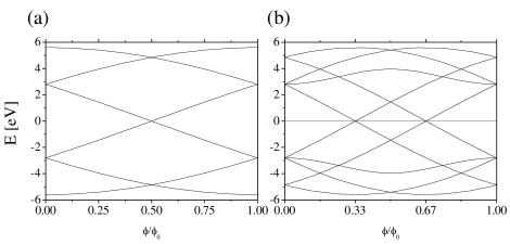
We focus here on the effect of the magnetic field on the electronic properties of TGQDs, quantum dots with broken sublattice symmetry. We illustrate the energy spectrum and its evolution with increasing magnetic field on a TGQD with $N=97$ carbon atoms. Fig. 1 shows the energy spectrum and it’s evolution in the magnetic field obtained by numerical diagonalization of the Hamiltonian, Eq. (1).

Figure 1: Left: Energy spectrum of triangular graphene quantum dot with $N=97$ atoms and $N_{ed}=7$ degenerate zero-energy states in the absence of a magnetic field. Right: the evolution of the spectrum from the left in a magnetic flux. The degenerate zero-energy shell is immune to the magnetic field. The states from the conduction and valence bands, labeled by I and II, respectively, crosses for $\phi/\phi_{0}\simeq 0.11$, closing the energy gap.

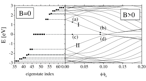
At $B=0$ there are $N_{deg}=7$ degenerate states at zero energy or Fermi level. The number of states is equal to the difference between the number of $A$ and $B$ atoms Potasz+10 . The states belonging to the degenerate shell are primarily localized at the edge of the triangle and are entirely localized on one sublattice, say A, as shown in Fig. 2(c).

The evolution of the energy spectrum as a function of the magnetic field is shown on the right hand side of Fig. 1. The spectrum is symmetric with respect to $E=0$ due to electron-hole symmetry. This symmetry is broken when hoppings to the second nearest neighbors in Hamiltonian,Eq. (1), are included. The highest valence state and the lowest conduction state with $E=\pm 1.57$ eV, which in the absence of the magnetic field are each doubly degenerate, split in the presence of a magnetic field. The state labeled by II from the valence band increases and the state labeled by I from the conduction band decreases its energy with increasing magnetic field, closing the energy gap. Around $\phi/\phi_{0}\simeq 0.11$ these states reach Fermi level at $E=0$.

The explanation of why the energy gap closes in a magnetic field can be found by considering Dirac Fermions in bulk graphene. Novoselov+Geim+05 ; Zhang+Tan+05 . We focus on one of two Fermi points, say $K$ point. Following Refs. mcclure+56, ; Toke et al., 2006 the energy spectrum of Dirac Hamiltonian in the presence of magnetic field is given by

$$E_{n}=\pm\sqrt{2\hbar v_{F}eB_{z}|n|/c},$$ (3)

where $v_{F}$ is Fermi velocity, $c$ speed of light, and $n$ Landau level index. The $\pm$ sign corresponds to electron (hole) Landau levels. A unique property of the energy spectrum is the existence of the $n=0$ Landau level with energy $E=0$, constant for all magnetic fields. When the magnetic field is applied to graphene quantum dots, discrete energy levels evolve into the degenerate Landau Levels for Dirac Fermions. Thus, some levels have to evolve into the $0$-th Landau level, closing the energy gap as shown in Fig. 1. Another feature of the $0$-th Landau level is that the wavefunctions are localized on only one sublattice, similar to the zero-energy states in TGQDPotasz+10 .

We note in Fig. 1 that the zero-energy degenerate shell is immune to the magnetic field as is the $n=0$ Landau level. This is certainly different from electronic states in semiconductor quantum dots, where $\sim B^{2}$ dependence is observed. raymond+04

These comments are now illustrated by examining wavefunctions of a TGQD in a magnetic field. We investigate the evolution of the probability density of the wavefunction corresponding to state I, bottom of the conduction band, from Fig. 1, and the total probability density of the zero-energy degenerate shell in a magnetic field. For state I, probability densities at low and high magnetic field values are shown in Fig. 2(a) and (b), respectively. We note that due to the electron-hole symmetry, an identical evolution for the state II from Fig. 1 (not shown here) occurs. Eigenfunctions of states with energy $-|E|$ and $+|E|$ differ only by a sign of a coefficient on sublattice $B$ indicated by filled circles in Fig. 2, giving identical electronic densities. For $\phi/\phi_{0}\simeq 0.01$, Fig. 2(a), the state I is mostly localized at the center of the dot. With increasing magnetic field, it starts to occupy the edge sites, shown for $\phi/\phi_{0}\simeq 0.08$. We note that for arbitrary magnetic field this state is equally shared over two sublattices, i.e, has $50\%$ sublattice content. In Fig. 2(c) and (d) the evolution of the total electronic density of the degenerate zero-energy shell is shown. The electronic density of the degenerate shell is obtained by summing over all $N_{deg}=7$ states. Initially, degenerate states are strongly localized on edges, shown in Fig. 2(c) for $\phi/\phi_{0}\simeq 0.01$. When the magnetic field increases, these states move slightly towards the center of the triangle, shown in Fig. 2(d) for $\phi/\phi_{0}\simeq 0.08$. We note that even in the presence of an external magnetic field states from the degenerate shell are still localized on only one type of atoms, sublattice A, indicated by open circles in Fig. 2.

Figure 2: (Color online) The evolution of electronic densities in a magnetic field of the lowest state from the conduction band labeled by $I$, (a) and (b), and the degenerate shell of $N_{deg}=7$ energy levels (the sum of electronic densities of all $N_{deg}=7$ degenerate states), (c) and (d). The radius of gray circles is proportional to the electronic probability density on a given site. (a) The state $I$ for $\phi/\phi_{0}\simeq 0.01$ is mostly localized in the center of the dot and with increasing magnetic field starts to occupy also edges, shown for $\phi/\phi_{0}\simeq 0.08$ in (b). (c) The degenerate states for $\phi/\phi_{0}\simeq 0.01$ are strongly localized on edges and for $\phi/\phi_{0}\simeq 0.08$ move slightly to the center of the triangle, shown in (d).

III.2 Analytical solution for zero-energy states

Fig. 1 shows that numerical diagonalization of the tb-Hamiltonian gives the zero-energy states immune to external magnetic field. We will now prove this analytically. Our first goal is to show the existence of and find an expression for zero-energy eigenstates in the presence of a magnetic field. The zero energy states, if they exist, must be solutions of the singular eigenvalue problem,

$$H_{TB}\Psi=0,$$ (4)

where the Hamiltonian $H_{TB}$ is given by Eq. (1). There is no coupling between two sublattices and the solution can be written separately for $A$-type and $B$-type of atoms. We first focus on sublattice $A$ with an eigenfunction given by

$$|\Psi^{A}\rangle=\sum_{j}C_{j}a^{\dagger}_{j}|0\rangle=\sum_{j}C_{j}|\phi_{j}^{A}\rangle,$$ (5)

where $C_{j}$ are expansion coefficients of eigenstates written in a basis of $p_{z}$ orbitals $\phi_{j}^{A}$ localized on $A$-type site $j$ for either spin state omitted in what follows.

According to Eq. 4, the coefficients $C_{j}$ corresponding to one type orbitals localized around the second type site $i$ obey

$$t\sum_{\left\langle i,j\right\rangle}C_{j}e^{i\varphiup_{ij}}=0,$$ (6)

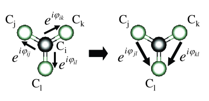
where the summation is over $j$-th nearest neighbors of an atom $i$. In other words, the sum of coefficients multiplied by a phase $e^{i\varphiup_{ji}}$ gained by going from one type site $i$ to the other type site $j$ around each site $i$ must vanish. For the $i$-th $B$-type site plotted on the left in Fig. 3, Eq. (6) gives

$$C_{j}e^{i\varphiup_{ij}}+C_{k}e^{i\varphiup_{ik}}+C_{l}e^{i\varphiup_{il}}=0,$$ (7)

where phases $\varphiup_{ij},\varphiup_{ik},\varphiup_{il}$ are given by Eq. (2). Using a fact that $\varphiup_{ik}=-\varphiup_{ki}$ for arbitrary $i$ and $k$, Eq. (7) can be written as

$$C_{l}=-\left(C_{j}e^{-i\varphiup_{jl}}+C_{k}e^{-i\varphiup_{kl}}\right),$$ (8)

where $\varphiup_{jl}=\varphiup_{ji}+\varphiup_{il}$ and $\varphiup_{kl}=\varphiup_{ki}+\varphiup_{il}$ correspond to phase changes going from $A$-type sites $k$ to $j$, and $l$ to $j$, respectively, through $B$-type site $i$ (see right part in Fig. 3). Thus, in analogy with the zero magnetic field case Potasz+10 , a coefficient from a given row can be expressed as a sum of two coefficients from an upper lying row, $C_{j}$ and $C_{k}$ on the right in Fig. 3. The effect of the magnetic field is incorporated in the extra phase gained by going from a given site from an upper row of atoms to a lower one. For a reason which will become clear later, instead of using indices $i$, each $A$-type site will be labeled by two integer numbers, ${i}=\{n,m\}$. The first index, $n$, corresponds to an atom number in a given row counted from left to right, and the second one, $m$, corresponds to the row number. Let us illustrate our methodology on a hexagonal benzene ring with three auxiliary $A$-type atoms with indices $C_{0,0}$, $C_{2,0}$ and $C_{0,2}$, shown in Fig. 4(a). Eq. (8) can be used to obtain coefficients $C_{0,1}$ from $C_{0,0}$ and $C_{1,0}$, and $C_{1,1}$ from $C_{1,0}$ and $C_{2,0}$. Next, using $C_{0,1}$ and $C_{1,0}$, one obtains coefficient $C_{0,2}$,

$$C_{0,2}=C_{0,0}e^{-i\varphiup_{1}}+C_{1,0}\left(e^{-i\varphiup_{2}}+e^{-i\varphiup_{3}}\right)+C_{2,0}e^{-i\varphiup_{4}},$$ (9)

with phase changes $\varphiup_{i}$, $i=1,2,3,4$, shown as black arrows in Fig. 4(a). The paths related to phase changes $\varphiup_{i}$ go through intermediate atomic sites, e.g., for $\varphiup_{1}$ the path goes from a site $C_{0,0}$ to $C_{0,1}$ through an intermediate $B$-type atomic site, and next from a site $C_{0,1}$ to $C_{0,2}$ through connecting $B$-type atomic site. According to Eq. (9) and Fig. 4(a), there is one path connecting $C_{0,0}$ and $C_{0,2}$, one connecting $C_{2,0}$ and $C_{0,2}$, but there are two paths around a hexagonal benzene ring connecting coefficients $C_{1,0}$ and $C_{0,2}$. We have shown that the coefficient in the bottom, $C_{0,2}$, can be expressed as a linear combination of coefficients from the top row, $C_{n,0}$. We will now demonstrate that all coefficient in arbitrary size triangles can be expressed in terms of coefficients $C_{n,0}$.

Figure 3: (Color online) Left: phase changes going from $B$-type site $i$ to three nearest neighbors $A$-type sites $j$, $k$, and $l$. The sum of three $A$-type coefficients multiplied by corresponding phase changes must vanish for zero-energy states. Right: phase changes going from $A$-type site $k$ to $j$, and $l$ to $j$. A coefficient from the bottom, $C_{l}$, can be expressed as a sum of coefficients from an upper row, $C_{j}$ and $C_{k}$, multiplied by corresponding phase change.

In Fig. 4(b) a small triangle with $N_{ed}=2$ atoms on the one edge is plotted. Three auxiliary atoms with coefficients $C_{0,0}$, $C_{3,0}$, and $C_{0,3}$ were added.

Figure 4: (Color online) (a) A hexagonal benzene ring with three auxiliary corner atoms added. Each $A$-type site is described by two numbers $\{n,m\}$. Black arrows indicate phase changes related to the paths going from an upper row of atoms, with indices $\{n,0\}$, to an atom from in the bottom, $C_{0,2}$. (b) Triangular zigzag graphene quantum dot with $N_{ed}=2$ atoms on one edge. There is one path going from site $C_{0,0}$ to $C_{0,3}$, and three paths going from site $C_{1,0}$ to $C_{0,3}$. The number of paths connecting a site $\{n,m\}$ with a site from the top $\{n+j,0\}$ can be described by binomial coefficient $N_{path}(n,m,n+j)={m\choose j}$, $0\leq j\leq m$.

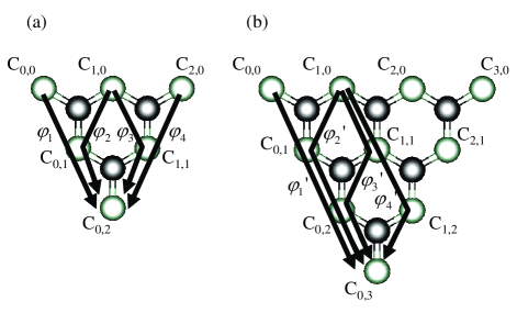
The total number of atoms is $N=16$. In a similar way to the procedure used to obtain Eq. (9), a coefficient $C_{0,3}$ can be expressed as a sum of coefficients from the top. Here, from coefficients $C_{0,0}$ and $C_{3,0}$ to $C_{0,3}$ there is only one path for each coefficient, and three paths for each coefficient connecting $C_{1,0}$ to $C_{0,3}$, and $C_{2,0}$ to $C_{0,3}$. For transparency, only for the first two coefficients from the left ($C_{0,0}$ and $C_{1,0}$) paths are plotted in Fig. 4(b). The number of paths from a given site in the upper row of atoms to lower lying atomic sites corresponds to numbers from a Pascal triangle, $\{1,2,1\}$ for coefficient $C_{0,2}$, shown in Fig. 4(a), and $\{1,3,3,1\}$ for coefficient $C_{0,3}$, shown for the first two coefficients from the left in Fig. 4(b). The number of paths connecting a site $\{n,m\}$ with a site from the top $\{n+j,0\}$ can be described by binomial coefficient $N_{path}(n,m,n+j)={m\choose j}$, $0\leq j\leq m$. The general form for an arbitrary coefficient expressed in coefficients from the top row can be written as

$$C_{n,m}=(-)^{m}\sum_{j=0}^{m}\sum_{i=1}^{m\choose j}C_{n+j,0}e^{-i\varphiup_{n+j}(i)},$$ (10)

where two numbers $n$ and $m$ satisfy condition $0<n,m<N_{ed}+1$, and $\varphiup_{n+j}(i)$ is a path-dependent phase change from a site $\{n+j,0\}$ to $\{n,m\}$. One can note that in the absence of a magnetic field $\varphiup_{n+j}(i)=0$ and Eq. (10) reduces to Eq.(2) from Ref.Potasz+10 .

The summation over all possible paths in Eq. (10) is not practical. We now show a way of reducing the number of paths to only one. We use the fact that a phase change corresponding to a closed path around a hexagon is by definition $\varphiup_{c}=2\pi\phi/\phi_{0}$. The sum of two exponential terms standing next to coefficient $C_{1,0}$ in Eq. (9) can be written as

$$e^{-i\varphiup_{2}}+e^{-i\varphiup_{3}}=\left(e^{i(\varphiup_{3}-\varphiup_{2})}+1\right)e^{-i\varphiup_{3}}=\left(e^{2\pi i\frac{\phi}{\phi_{0}}}+1\right)e^{-i\varphiup_{3}},$$ (11)

where $\varphiup_{3}-\varphiup_{2}=2\pi\phi/\phi_{0}$ is a closed path around a single hexagon, see Fig. 4(a). Similarly for three exponential terms corresponding to paths connecting $C_{10}$ and $C_{03}$, shown in Fig. 4(b), one can write

$$e^{-i\varphiup_{2}^{\prime}}+e^{-i\varphiup_{3}^{\prime}}+e^{-i\varphiup_{4}^{\prime}} = \left(e^{i(\varphiup_{4^{\prime}}-\varphiup_{2^{\prime}})}+e^{i(\varphiup_{4^{\prime}}-\varphiup_{3^{\prime}})}+1\right)e^{-i\varphiup_{4^{\prime}}}$$ (12)

$$= \left(e^{2\pi i(2\frac{\phi}{\phi_{0}})}+e^{2\pi i\frac{\phi}{\phi_{0}}}+1\right)e^{-i\varphiup_{4^{\prime}}},$$

where $(\varphiup_{4^{\prime}}-\varphiup_{2^{\prime}})$ circles two hexagons and $(\varphiup_{4^{\prime}}-\varphiup_{3^{\prime}})$ only one, see Fig. 4(b). Note that phases $\varphiup_{3}$ in Eq. (11) and $\varphiup_{4^{\prime}}$ in Eq. (12) correspond to paths going on the right edge of the triangle. The sum of exponential terms of type $e^{2\pi i(j\frac{\phi}{\phi_{0}})}$ with $j$-integer in Eq. (11) and Eq. (12) forms geometric series which can be written as

$$\sum_{j=0}^{k}e^{2\pi i(j\frac{\phi}{\phi_{0}})}=\frac{1-e^{2\pi i(k+1)\frac{\phi}{\phi_{0}}}}{1-e^{2\pi i\frac{\phi}{\phi_{0}}}},$$ (13)

with $k$ determined by the number of encircled benzene rings, and $k+1={m\choose j}$ is a number of paths connecting site $\{n+j,0\}$ to $\{n,m\}$, $k=1$ in Eq. (11) and $k=2$ in Eq. (12), see Fig. 4. Using Eq. (13), the number of paths in Eq. (10) can be reduced to only one. Eq. (10) can be written as

$$C_{n,m}=(-)^{m}\sum_{j=0}^{m}C_{n+j,0}\frac{1-e^{2\pi i{m\choose j}\frac{\phi}{\phi_{0}}}}{1-e^{2\pi i\frac{\phi}{\phi_{0}}}}e^{-i\varphiup_{n+j}},$$ (14)

where $\varphiup_{n+j}$ is the phase corresponding to the path on the right edge connecting site $\{n+j,0\}$ and $\{n,m\}$. The coefficients $C_{n,m}$ for all $A$-type atoms in the triangle are expressed as a linear combination of coefficients corresponding to atoms on one edge, i.e., $C_{j,0}$. There are $N_{ed}+2$ coefficients in an upper row of atoms, $C_{j,0}$, with $0<j<N_{ed}+1$, which gives $N_{ed}+2$ independent solutions. Applying three boundary conditions corresponding to auxiliary atoms, $C_{0,0}=C_{N_{ed}+1,0}=C_{0,N_{ed}+1}=0$, leaves only $N_{ed}-1$ solutions, which corresponds to the number of zero-energy states, similar to the result obtained in the absence of a magnetic field in Ref. Potasz+10, . We note that the solutions given by Eq. (14) are smooth functions of magnetic field, and exist for any value of $\phi$. Thus they do not include zero-energy solutions corresponding to the crossing of conduction and valence states with $E=0$, e. g., for $\phi/\phi_{0}\simeq 0.11$ for the triangular dot with $N_{ed}=8$ and $N=97$ atoms, see Fig. 1. We investigate this issue by analyzing $B$-type atoms.

III.3 Prediction of crossings of valence and conduction states with $E=0$

We consider the solution of Eq. (4) corresponding to wavefunction localized only on $B$-type atoms. In Fig. 5 the same structures as in Fig. 4 without auxiliary corner atoms are shown with coefficients assigned to $B$-type atoms. For simplicity, only one index for each coefficient is used.

Figure 5: (Color online) (a) A hexagonal benzene ring with coefficients $C_{i}$ assigned to each $B$-type site. Black arrows indicate phase changes related to the paths going from one $B$-type site to another. (b) Triangular zigzag graphene quantum dot with $N_{ed}=2$ atoms on the one edge. Black arrows indicate phase changes related to the paths going from one $B$-type site to another along triangular three edges. White arrows indicate phase changes related to the paths going through the center.

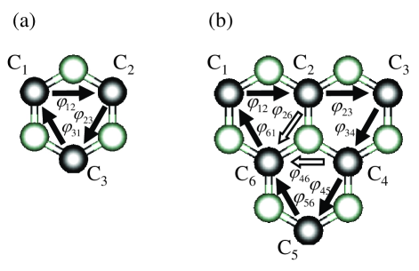
According to Eq. 6, for a benzene ring plotted in Fig. 5(a) we can write

$$C_{2}=-C_{1}e^{-i\varphiup_{12}},$$ (15)

$$C_{3}=-C_{2}e^{-i\varphiup_{23}},$$ (16)

$$C_{1}=-C_{3}e^{-i\varphiup_{31}},$$ (17)

where phase changes from site $i$ to $j$, $\varphiup_{ij}$, are indicated in Fig. 5(a). Eq. (15) can be substituted into Eq. (16), and next Eq. (16) into Eq. (17), giving

$$C_{1}=C_{1}(-1)^{3}e^{-i(\varphiup_{12}+\varphiup_{23}+\varphiup_{31})},$$ (18)

which is satisfied for arbitrary $C_{1}$. Eq. 18 leads to a following condition

$$\varphiup_{12}+\varphiup_{23}+\varphiup_{31}+\pi=2\pi k,$$ (19)

with $k=0,\pm 1,\pm 2,...$. A phase change in Eq. (19) corresponds to a closed path around a single hexagon, $\varphiup_{12}+\varphiup_{23}+\varphiup_{31}=2\pi\phi/\phi_{0}$. A condition for crossing of a valence and conduction states with $E=0$ is

$$\phi/\phi_{0}=k-1/2.$$ (20)

In order to confirm validity of Eq. (20), we show the energy spectrum of a benzene ring as a function of a magnetic field in Fig. 6(a). The crossing of energy levels at $E=0$ occurs for $\phi/\phi_{0}=1/2$, in agreement with Eq. (20).

We carry out a similar derivation for triangular zigzag graphene quantum dot with $N=13$ carbon atoms and $N_{ed}=2$ atoms on the one edge, shown in Fig. 5(b). A coefficient from the left upper corner, $C_{1}$, determines a coefficient $C_{2}$,

$$C_{2}=-C_{1}e^{-i\varphiup_{12}}.$$ (21)

Next, a coefficient $C_{3}$ can be determined by a coefficient $C_{2}$

$$C_{3}=-C_{2}e^{-i\varphiup_{23}}$$ (22)

and combining with Eq. (21) gives

$$C_{3}=(-1)^{2}C_{1}e^{-i(\varphiup_{12}+\varphiup_{23})}=(-1)^{2}C_{1}e^{-i\varphiup_{13}}.$$ (23)

Going in this way along the three edges of the triangle a closed loop, shown with black arrows in Fig. 5(b), can be created. In the

Figure 6: Energy spectrum as function of magnetic flux for (a) a hexagonal benzene ring and (b) a triangular graphene quantum dot with $N_{ed}=2$ atoms on the one edge and a total of $N=13$ atoms. A crossing of conduction and valence states with $E=0$ occurs for (a) $\phi/\phi_{0}=1/2$ and (b) $\phi/\phi_{0}=1/3$ and $\phi/\phi_{0}=2/3$.

case of $N_{ed}=2$ shown in Fig. 5(b), one goes through all $B$-type coefficients, while in larger triangles one goes only through outer coefficients. Thus, all outer $B$-type coefficients can be expressed by one chosen coefficient, $C_{1}$ in this case. The loop from Fig. 5(b) can be written

$$C_{1}=(-1)^{6}C_{1}e^{-i(\varphiup_{16}+\varphiup_{61})}=C_{1}e^{6\pi i-2\pi i(3\phi/\phi_{0})},$$ (24)

where the phase change $\varphiup_{16}=\sum_{i}^{5}\varphiup_{i,i+1}$, and we used a fact that the total phase change corresponds to a closed loop around three benzene rings, $\varphiup_{16}+\varphiup_{61}=2\pi(3\phi/\phi_{0})$. Eq. (24) gives a condition

$$2k\pi=6\pi-6\pi\phi/\phi_{0},$$ (25)

and finally

$$\phi/\phi_{0}=\frac{3-k}{3}.$$ (26)

with $k=0,\pm 1,\pm 2,...$. Eq. (26) can be extended to different size triangles. The number of benzene rings in a triangle is $N_{b}=N_{ed}(N_{ed}+1)/2$, and Eq. (26) can be written as

$$\phi/\phi_{0}=\frac{3N_{ed}-2k}{N_{ed}\left(N_{ed}+1\right)}.$$ (27)

For the triangle with $N_{ed}=2$, Eq. (26) predicts crossings for $\phi/\phi_{0}=0,\pm 1/3,\pm 2/3,1,..$ but according to Fig. 6(b) there are no crossings for $\phi/\phi_{0}=0$ and $\phi/\phi_{0}=1$. This is related to an extra condition in the center of the triangle, for coefficients $C_{2}$, $C_{4}$, and $C_{6}$. Phase changes between these coefficients are indicated by white arrows in Fig. 5(b). We can write

$$C_{6}=-\left(C_{2}e^{-i\varphiup_{26}}+C_{4}e^{-i\varphiup_{46}}\right)$$ (28)

and also

$$C_{6}=-C_{1}e^{-i(-\varphiup_{61})}=-C_{1}e^{i\varphiup_{61}},$$ (29)

$$C_{2}=-C_{1}e^{-i\varphiup_{12}},$$

$$C_{4}=(-1)^{3}C_{1}e^{-i\varphiup_{14}},$$

where the phase change $\varphiup_{14}=\sum_{i}^{3}\varphiup_{i,i+1}$. Combining Eq. (28) and Eq. (29) we get

$$-C_{1}e^{i\varphiup_{61}}=-\left(-C_{1}e^{-i(\varphiup_{12}+\varphiup_{26})}+(-1)^{3}C_{1}e^{-i(\varphiup_{14}+\varphiup_{46})}\right),$$ (30)

which gives

$$-1=e^{-i(\varphiup_{12}+\varphiup_{26}+\varphiup_{61})}+e^{-i(\varphiup_{14}+\varphiup_{46}+\varphiup_{61})}.$$ (31)

With help of Fig. 5(b), we can notice $\varphiup_{12}+\varphiup_{26}+\varphiup_{61}=2\pi\phi/\phi_{0}$ and $\varphiup_{14}+\varphiup_{46}+\varphiup_{61}=2\pi(2\phi/\phi_{0})$. Thus, we can write

$$1+e^{-2\pi i\phi/\phi_{0}}+e^{-2\pi i(2\phi/\phi_{0})}=0$$ (32)

or using a sum of geometric series

$$\frac{1-e^{-2\pi i(3\phi/\phi_{0})}}{1-e^{-2\pi i\phi/\phi_{0}}}=0.$$ (33)

Eq. (33) gives a solution for $-2\pi(3\phi/\phi_{0})=2\pi k$, $k$-integer, and finally $\phi/\phi_{0}=-k/3$, but with an extra condition $\phi/\phi_{0}\neq l$, with $l=0,\pm 1,\pm 2,..$ due to a denominator. This is in agreement with Fig. 6(b). We note that for all triangles, the prediction of crossings of conduction and valence states with $E=0$ given by Eq. (27) has to be supported by extra conditions from equations for coefficients from the center of the triangle. For example, for the triangle with $N_{ed}=8$, the first crossing occurs for $\phi/\phi_{0}=1/9$, while incomplete condition given by Eq. (27) predicts the first crossing for $\phi/\phi_{0}=1/36$, and the fourth crossing for $\phi/\phi_{0}=1/9$.

Figure 7: Energy spectrum as a function of magnetic flux for different sizes of triangular zigzag quantum dots, showing that first zero energy crossing occurs at $\phi/\phi_{0}=1/(N_{ed}+1)$.

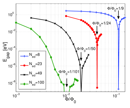
An interesting prediction of Eq.(26) is that the zero energy crossing values of $\phi/\phi_{0}$ should scale as $\sim 1/N_{ed}$ for large $N_{ed}$. In order to check numerically the size dependence of the position of the first crossing, in Fig. 7 we show the energy gap as a function of $\phi/\phi_{0}$ for different $N_{ed}$ obtained by diagonalization of the tight-binding Hamiltonian. Strikingly, we find that the first crossing always occurs at $\phi/\phi_{0}=1/(N_{ed}+1)$ for all the values of $N_{ed}$ that we have looked at. This is consistent with Eq.(26) with $k=N_{ed}$. Extrapolating this result to larger structures, it would take a magnetic field value of $\sim 10$ Tesla for a quantum dot with $N_{ed}=4000$ to reach the first zero energy crossing.

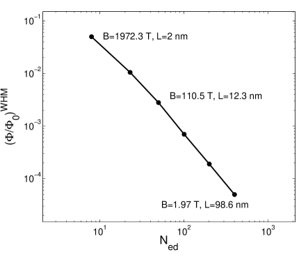
However, for large quantum dots ($N_{ed}>100$, or linear size $L>25$ nm) it becomes increasingly difficult to pinpoint numerically the position of the zero energy crossing due to smallness of the energy gap around the crossing and numerical accuracy. Another quantity of interest is the width at half maximum (WHM) of the flux dependence of the energy gap. In Fig. 8 we plot the WHM as a function of $N_{ed}$. Unlike the first crossing point which scales as $N_{ed}^{-1}$, the WHM scales as $\sim N_{ed}^{-2}$ for large $N_{ed}$, thus much faster. In Fig. 8 the largest structure that we looked at has $N=161601$ atoms ($N_{ed}=401$, $L=98.6$ nm) for which the WHM occurs at a magnetic field value of $B=1.97$ Tesla.

Figure 8: Width at half maximum of the flux dependence of the energy gap as a function of $N_{ed}$, showing a $\sim N_{ed}^{-2}$ dependence at large $N_{ed}$. For few points, corresponding magnetic field values and linear sizes are given in Tesla and nm respectively.

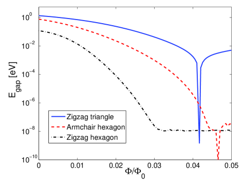
IV SHAPE AND EDGE DEPENDENCE OF THE ENERGY GAP IN A MAGNETIC FIELD

We discussed above the magnetic field closing of the energy gap in triangular graphene quantum dots. In Fig. 9, we analyze the evolution of the energy gap in graphene quantum dots with different shapes and edges in a perpendicular magnetic field. The energy gaps as a function of a magnetic field obtained by diagonalizing Hamiltonian given by Eq. (1) are shown for three different types of quantum dots; zigzag triangle, zigzag hexagon, and armchair hexagon. All three structures have similar sizes, consisting of $N\simeq 600$ atoms with area $S\simeq 14$ nm². The energy gap corresponds to the difference between the energy of the lowest state from the empty conduction states and the highest state from the doubly occupied valence states. In the absence of magnetic field, the zigzag triangular graphene quantum dot has a significantly larger gap then for hexagonal armchair and zigzag dots as discussed in Ref.Guclu+10, . The functional form of the gap closure of different types of structures has significant differences as well, as seen in Fig. 9. When the magnetic field increases, the energy gap closes for all structures. Although the hexagonal zigzag structure has slightly smaller size, the gap decays fastest showing a different behavior than the $\sim N_{ed}^{-2}$ scaling shown earlier for the triangular zigzag structure. Moreover, after reaching a plateau close to zero ($\sim 10^{-8}$) the hexagonal zigzag quantum dot shows no more structures, i.e. no zero energy crossings, unlike the two other quantum dots. We note that for the hexagonal zigzag structure the gap comes from closure of the edge-like states (which have finite energies unlike the triangular zigzag structure). This shows that the zero crossings are characteristics of bulk-like states.

Figure 9: The energy gap as function of the magnetic flux for triangular zigzag quantum dot with $N=622$ atoms (solid line), hexagonal armchair quantum dot with $N=546$ atoms (dashed line), hexagonal zigzag quantum dot with $N=600$ atoms (dot-dashed line).

V CONCLUSIONS

The electronic properties of triangular graphene quantum dots with zigzag edges and broken sublattice symmetry in the presence of perpendicular external magnetic field were described. It was shown that the degenerate shell of zero-energy states in the middle of the energy gap is immune to the magnetic field in analogy to the $n=0$ Landau level of bulk graphene. An analytical solution for zero-energy states in the magnetic field was derived. The energy gap was shown to close with increasing magnetic field, reaching zero at special values of the magnetic field. The gap closing was found independent of quantum dot size, shape, and edge termination.

References

- (1) P. R. Wallace, Phys. Rev. 71, 622 (1947).
- (2) K. S. Novoselov, A. K. Geim, S. V. Morozov, D. Jiang, Y. Zhang, S. V. Dubonos, I. V. Grigorieva, and A. A. Firsov, Science 306, 666 (2004).
- (3) K. S. Novoselov, A. K. Geim, S. V. Morozov, D. Jiang, M. I. Katsnelson, I. V. Grigorieva, S. V. Dubonos, and A. A. Firsov, Nature 438, 197 (2005).
- (4) Y. B. Zhang, Y. W. Tan, H. L. Stormer, and P. Kim, Nature 438, 201 (2005).
- (5) Y. W. Son, M. L. Cohen, and S. G. Louie, Phys. Rev. Lett. 97, 216803 (2006).
- (6) M. L. Sadowski, G. Martinez, M. Potemski, C. Berger, and W. A. de Heer, Phys. Rev. Lett. 97, 266405 (2006).
- (7) A. K. Geim and K. S. Novoselov, Nat. Mater. 6, 183 (2007).
- (8) A. Rycerz, J. Tworzydlo, and C. W. Beenakker, Nature Phys. 3, 172 (2007).
- (9) F. Xia, T. Mueller, Y.-M. Lin, A. Valdes-Garcia, and P. Avouris, Nat. Nanotechnol. 4, 839 (2009).
- (10) T. Mueller, F. Xia, and P. Avouris, Nat. Photon. 4, 297 (2010).
- (11) A. H. C. Neto, F. Guinea, N. M. R. Peres, K. S. Novoselov, and A. K. Geim, Rev. of Mod. Phys. 81, 109 (2009).
- (12) A. H. Abergel, G. Apalkov, Y. P. Berashevich, V. Ziegler, and F. Chakraborty, Adv. in Phys. 59 , 261 (2010).
- (13) A. H. Rozhkov, G. Giavaras, Y. P. Bliokh, V. Freilikher, and F. Nori, Phys. Rep. 81 , 195414 (2011).
- (14) X. Li, X. Wang, L. Zhang, S. Lee, and H. Dai, Science 319, 1229 (2008).
- (15) L. A. Ponomarenko, F. Schedin, M. I. Katsnelson, R. Yang, E. W. Hill, K. S. Novoselov, and A. K. Geim, Science 320, 356 (2008).
- (16) L. Ci, Z. Xu, L. Wang, W. Gao, F. Ding, K. F. Kelly, B. I. Yakobson, and P. M. Ajayan, Nano Res 1, 116 (2008).
- (17) Y. You, Z. Ni, T. Yu, and Z. Shena, Appl. Phys. Lett. 93, 163112 (2008).
- (18) S. Schnez, F. Molitor, C. Stampfer, J. Güttinger, I. Shorubalko, T. Ihn, and K. Ensslin, Appl. Phys. Lett. 94, 012107 (2009).
- (19) K. A. Ritter and J. W. Lyding, Nat Mater. 8, 235 (2009).
- (20) X. Jia, M. Hofmann, V. Meunier, B. G. Sumpter, J. Campos-Delgado, J. M. Romo-Herrera, H. Son, Y.-P. Hsieh, A. Reina, J. Kong, M. Terrones, and M. S. Dresselhaus, Science 323, 1701 (2009).
- (21) L. C. Campos, V. R. Manfrinato, J. D. Sanchez-Yamagishi, J. Kong, and P. Jarillo-Herrero, Nano Lett. 9, 2600 (2009).
- (22) S. Neubeck, Y. M. You, Z. H. Ni, P. Blake, Z. X. Shen, A. K. Geim, and K. S. Novoselov, Appl. Phys. Lett. 97, 053110 (2010).
- (23) L. P. Bir and Ph. Lambin, Carbon 48, 2677 (2010).
- (24) E. Cruz-Silva, A. R. Botello-Mendez, Z. M. Barnett, X. Jia, M. S. Dresselhaus, H. Terrones, M. Terrones, B. G. Sumpter, and V. Meunier, Phys. Rev. Lett. 105, 045501 (2010).
- (25) R. Yang, L. Zhang, Y. Wang, Z. Shi, D. Shi, H. Gao, E. Wang, and G. Zhang, Adv. Mater. 22, 4014 (2010).
- (26) B. Krauss, P. Nemes-Incze, V. Skakalova, L. P. Bir, K. von Klitzing, and J. H. Smet, Nano Lett. 10, 4544 (2010).
- (27) L. Zhi and K. Müllen, J. Mater. Chem. 18, 1472 (2008).
- (28) M. Treier, C. A. Pignedoli, T. Laino, R. Rieger, K. Müllen, D. Passerone, and R. Fasel, Nat. Chem. 3, 61 (2010).
- (29) M. L. Mueller, X. Yan, J. A. McGuire, and L. Li, Nano Lett. 10, 2679 (2010).
- (30) Y. Morita, S. Suzuki, K. Sato, and T. Takui, Nat. Chem. 3, 197 (2011).
- (31) J. Lu, P. S. E. Yeo, C. K. Gan, P. Wu, and K. P. Loh, Nat. Nanotechnol. 6, 247 (2011).
- (32) X. Chen, S. Liu, L. Liu, X. Liu, X. Liu, and L. Wang, Appl. Phys. Lett. 100, 163106 (2010).
- (33) T. Yamamoto, T. Noguchi, and K. Watanabe, Phys. Rev. B 74, 121409 (2006).
- (34) Z. Z. Zhang, K. Chang, and F. M. Peeters, Phys. Rev. B 77 , 235411 (2008).
- (35) A. D. Güçlü, P. Potasz, and P. Hawrylak, Phys. Rev. B 82 , 155445 (2010).
- (36) K. Nakada, M. Fujita, G. Dresselhaus, and M. S. Dresselhaus, Phys. Rev. B 54, 17954 (1996).
- (37) M. Fujita, K. Wakabayashi, K. Nakada, and K. Kusakabe, J. Phys. Soc. Jpn. 65, 1920 (1996).
- (38) Y. Son, M. L. Cohen, and S. G. Louie, Nature 444, 347 (2006).
- (39) M. Ezawa, Phys. Rev. B 73 , 045432 (2006).
- (40) M. Ezawa, Phys. Rev. B 76 , 245415 (2007).
- (41) J. Fernandez-Rossier and J. J. Palacios, Phys. Rev. Lett. 99, 177204 (2007).
- (42) J. Akola, H. P. Heiskanen, and M. Manninen, Phys. Rev. B 77 , 193410 (2008).
- (43) W. L. Wang, O. V. Yazyev, S. Meng, and E. Kaxiras, Phys. Rev. Lett. 102, 157201 (2009).
- (44) M. Wimmer, A. R. Akhmerov and F. Guinea, Phys. Rev. B 82 045409 (2010).
- (45) P. Potasz, A. D. Güçlü, and P. Hawrylak, Phys. Rev. B 81 , 033403 (2010).
- (46) O. Voznyy, A. D. Güçlü, P. Potasz, and P. Hawrylak, Phys. Rev. B 83, 165417 (2011).
- (47) M. Ezawa, Physica E 42, 703 (2010).
- (48) W. L. Wang, S. Meng, and E. Kaxiras, Nano Letters 8, 241 (2008).
- (49) A. D. Güçlü, P. Potasz, O. Voznyy, M. Korkusinski, and P. Hawrylak, Phys. Rev. Lett. 103 , 246805 (2009).
- (50) O. V. Yazyev, Rep. Prog. Phys. 73, 056501 (2010).
- (51) H. Y. Chen, V. Apalkov, and T. Chakraborty, Phys. Rev. Lett. 98, 186803 (2007).
- (52) S. Schnez, K. Ensslin, M. Sigrist, and T. Ihn, Phys. Rev. B 78, 195427 (2008).
- (53) P. Recher, B. Trauzettel, A. Rycerz, Ya. M. Blanter, C. W. J. Beenakker, and A. F. Morpurgo, Phys. Rev. B 76, 235404 (2007).
- (54) D. S. L. Abergel, V. M. Apalkov, and T. Chakraborty, Phys. Rev. B 78, 193405 (2008).
- (55) J. Wurm, M. Wimmer, H. U. Baranger, and K. Richter, Semicond. Sci. Technol. 25, 034003 (2010).
- (56) J. Guttinger, C. Stampfer, F. Libisch, T. Frey, J. Burgdorfer, T. Ihn, and K. Ensslin, Phys. Rev. Lett. 103, 046810 (2009).
- (57) D. A. Bahamon, A. L. C. Pereira, and P. A. Schulz, Phys. Rev. B 79, 125414 (2009).
- (58) F. Libisch, S. Rotter, J. Güttinger, C. Stampfer, and J. Burgdörfer, Phys. Rev. B 81, 245411 (2010).
- (59) M. Grujic, M. Zarenia, A. Chaves, M. Tadic, G. A. Farias, and F. M. Peeters, Phys. Rev. B 84, 205441 (2011).
- (60) M. Zarenia, A. Chaves, G. A. Farias, and F. M. Peeters, Phys. Rev. B 84, 245403 (2011).
- (61) I. Romanovsky, C. Yannouleas, and U. Landman, Phys. Rev. B 83 , 045421 (2011).
- (62) I. Romanovsky, C. Yannouleas, and U. Landman, Phys. Rev. B 86 , 165440 (2012).
- (63) P. Potasz, A. D. Güçlü, and P. Hawrylak, Acta Phys. Pol. A 116 , 832 (2009).
- (64) R. Saito, G. Dresselhaus, and M. S. Dresselhaus, Physical Properties of Carbon Nanotubes (Imperial College, London(1998).
- (65) R. E. Peierls, Z. Phys. 80, 763 (1933).
- Toke et al. (2006) C. Toke P. E. Lammert, V. H. Crespi, and J. K. Jain, Phys. Rev. B 74, 235417 (2006).
- (67) J. W. McClure, Phys. Rev. 104, 666 (1956).
- (68) S. Raymond, S. Studenikin, A. Sachrajda, Z. Wasilewski, S. J. Cheng, W. Sheng, P. Hawrylak, A. Babinski, M. Potemski, G. Ortner, and M. Bayer, Phys. Rev. Lett. 92, 187402 (2004).