Sine–Gordon Solitons, Kinks and Breathers as Physical Models of Nonlinear Excitations in Living Cellular Structures

Abstract

Nonlinear space-time dynamics, defined in terms of celebrated ‘solitonic’ equations, brings indispensable tools for understanding, prediction and control of complex behaviors in both physical and life sciences. In this paper, we review sine–Gordon solitons, kinks and breathers as models of nonlinear excitations in complex systems in physics and in living cellular structures, both intra–cellular (DNA, protein folding and microtubules) and inter–cellular (neural impulses and muscular contractions).
 

Key words: Sine–Gordon solitons, kinks and breathers, DNA, Protein folding, Microtubules, Neural conduction, Muscular contraction

1 Introduction

In spatiotemporal dynamics of complex nonlinear systems (see [1, 2, 3, 4]), Sine–Gordon equation (SGE) is, together with Korteweg–deVries (KdV) and nonlinear Schrödinger (NLS) equations, one of the celebrated nonlinear-yet-integrable partial differential equations (PDEs), with a variety of traveling solitary waves as solutions (see Figures 1 and 2, as well as the following basic references: [5, 6, 7, 8, 9, 10, 11]). In complex physical systems, SGE solitons, kinks and breathers appear in various situations, including propagation of magnetic flux (fluxons) in long Josephson junctions [14, 15], dislocations in crystals [16, 17], nonlinear spin waves in superfluids [14], and waves in ferromagnetic and anti-ferromagnetic materials [18, 19] – to mention just a few application areas.

In this paper, we review physical theory of sine–Gordon solitons, kinks and breathers, as well as their essential dynamics of nonlinear excitations in living cellular structures, both intra–cellular (DNA, protein folding and microtubules) and inter–cellular (neural impulses and muscular contractions).

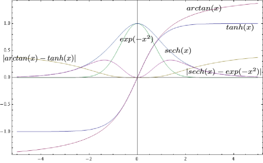
Figure 1: Basic static examples of kinks: $\mathop{\mathrm{t}anh}(x),~{}\mathop{\mathrm{a}rctan}(x)$ and bell–shaped solitons: $\mathop{\mathrm{s}ech}(x),~{}\mathop{\mathrm{e}xp}(-x^{2})$,  together with their (absolute) differences; plotted in $Mathematica^{TM}$.

We show that sine–Gordon traveling waves can give us new insights even in such long–time established and Nobel–Prize winning living systems as the Watson–Crick double helix DNA model and the Hodgkin–Huxley neural conduction model.

2 Physical theory of sine–Gordon solitons, kinks and breathers

In this section, we give the basic theory of the sine–Gordon equation (and the variety of its traveling–wave solutions), as spatiotemporal models of nonlinear excitations in complex physical systems.

2.1 Sine–Gordon equation (SGE)

SGE is a real-valued, hyperbolic, nonlinear wave equation defined on $\mathbb{R}^{1,1}$, which appears in two equivalent forms (using standard indicial notation for partial derivatives: $\phi_{zz}=\partial_{z}^{2}\phi=\partial^{2}\phi/\partial x^{z}$):

• In the (1+1) space-time $(x,t)-$coordinates, the SGE reads:

  $$\phi_{tt}=\phi_{xx}-\sin\phi,\qquad\text{{or}\qquad}\phi_{tt}(x,t)=\phi_{xx}(x,t)-\sin\phi(x,t),$$ (1)

  which shows that it is a nonlinear extension of the standard linear wave equation: $\phi_{tt}=\phi_{xx}.$ The solutions $\phi(x,t)$ of (1) determine the internal Riemannian geometry of surfaces of constant negative scalar curvature $R=-2,$ given by the line-element:

  $$ds^{2}=\sin^{2}\left(\frac{\phi}{2}\right)dt^{2}+\cos^{2}\left(\frac{\phi}{2}\right)dx^{2},$$

  where the angle $\phi$ describes the embedding of the surface into Euclidean space $\mathbb{R}^{3}$ (see [5]). A basic solution of the SGE (1) is:

  $$\phi(x,t)=4\arctan\left[\exp\left(\pm\frac{x-vt}{\sqrt{1-v^{2}}}\right)\right],$$ (2)

  describing a soliton moving with velocity $0\leq v<1$ and changing the phase from 0 to 2$\pi$ (kink, the case of $+$ sign) or from 2$\pi$ to 0 (anti-kink, the case of $-$ sign).

• In the (1+1) light-cone $(u,v)-$coordinates, defined by: $u=(x+t)/2,\,v=(x+t)/2$, in which the line-element (depending on the angle $\phi$ between two asymptotic lines: $u=\mathrm{const},v=\mathrm{const}$) is given by:

  $$ds^{2}=du^{2}+2\cos\phi\,du\,dv+dv^{2},$$

  the SGE describes a family of pseudo-spherical surfaces with constant Gaussian curvature $K=-1,$ and reads:

  $$\phi_{uv}=\sin\phi\,,\qquad\text{{or}\qquad}\phi_{uv}(u,v)=\sin\phi(u,v).$$ (3)

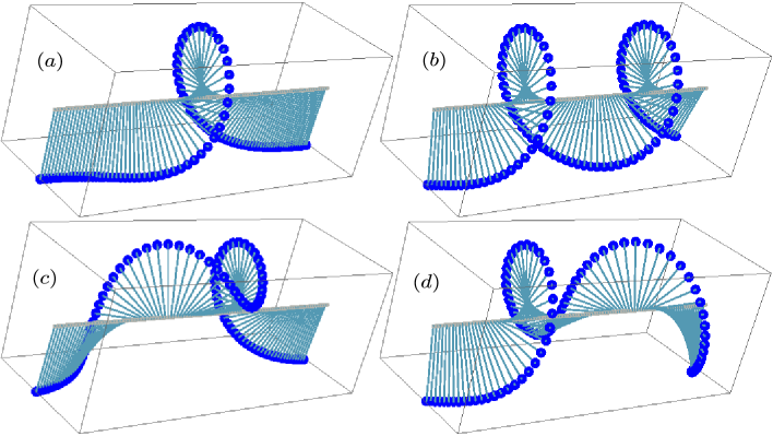
Figure 2: Basic solitary SGE–solutions, simulated in $Mathematica$ as systems of spring-coupled torsional pendula: (a) single soliton: $\phi(x,t)=4\arctan\left(\exp\frac{x-vt}{1-v^{2}}\right);$ (b) soliton–soliton collision: $\phi(x,t)=4\arctan\left(\frac{v\sinh\frac{x}{1-v^{2}}}{\cosh\frac{vt}{1-v^{2}}}\right);$ (c) soliton–antisoliton collision: $\phi(x,t)=4\arctan\left(\frac{\sinh\frac{vt}{1-v^{2}}}{v\cosh\frac{x}{1-v^{2}}}\right);$ and (d) single breather: $\phi(x,t)=4\arctan\left(\frac{\sin\frac{vt}{1-v^{2}}}{v\cosh\frac{x}{1-v^{2}}}\right)$ (modified and adapted from [13]).

A typical, spatially-symmetric, boundary-value problem for (1) is defined by:

$$x \in [-L,L]\subset\mathbb{R},\qquad\left(t\in\mathbb{R}^{+}\right),\hskip 48.36958pt$$

$$\phi(x,0) = f(x),\qquad\phi_{t}(x,0)=0,\qquad\phi(-L,t)=\phi(L,t),$$

where $f(x)\in\mathbb{R}$ is an axially-symmetric function (e.g., Gaussian or sech, see Figure 3).

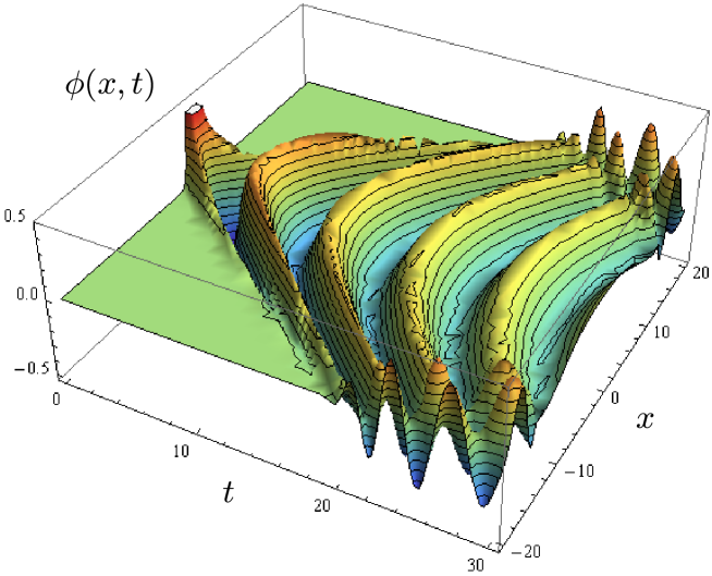
Figure 3: Numerical solution of the SGE (1) in $Mathematica$, using numerical ODE/PDE integrator NDSolve, with the following data (including the Gaussian initial state, zero initial velocity and symmetric boundary condition): $x\in[-20,20],~{}~{}t\in[0,30],~{}~{}\phi(x,0)=\exp({-x^{2}}),~{}~{}\phi_{t}(x,0)=0,~{}~{}\phi(-20,t)=\phi(20,t)$. The waves oscillate around the zero plane and increase their width with time. Both near-periodicity and nonlinearity of the time evolution are apparent.

Bäcklund transformations (BT) for the SGE (1) were devised in 1880s in Riemannian geometry of surfaces and are attributed to Bianchi and Bäcklund (see, e.g. [25]). They have the form:

$$\frac{1}{2}(\phi+\varphi)_{\xi}=\alpha\sin\frac{\phi-\varphi}{2},\qquad\frac{1}{2}(\phi-\varphi)_{\eta}=\frac{1}{\alpha}\sin\frac{\phi+\varphi}{2},$$ (4)

where both $\phi$ and $\varphi$ are solutions of the SGE (1), and can be viewed as a transformation of the SGE into itself. BT (4) allows one to find a 2-parameter family of solutions, given a particular solution $\phi_{0}$ of (1). For example, consider the trivial solution $\phi=0$ that, substituted into (4), gives:

$$\varphi_{\xi}=-2\alpha\sin\frac{\varphi}{2},\qquad\varphi_{\eta}=-\frac{2}{\alpha}\sin\frac{\varphi}{2},$$

which, by integration, gives:

$$2\alpha\xi=-2\ln(\tan\frac{\varphi}{4})+p(\eta),\qquad\frac{2}{\alpha}\eta=-2\ln(\tan\frac{\varphi}{4})+p(\xi),$$

from which the following new solution is generated:

$$\varphi=4\arctan\left[\exp(-\alpha\xi-\frac{1}{\alpha}\eta+\mathrm{const})\right].$$

The sine–forcing term in the SGE can be viewed as a nonlinear deformation: $\phi\rightarrow\sin\phi,$ of the linear forcing term in the Klein–Gordon equation (KGE, a vacuum linearization of the SGE), which is commonly used for describing scalar fields (quantum) field theory:

$$\phi_{tt}=\phi_{xx}-\phi,$$ (5)

This, in turn, implies that (as a field equation) SGE can be derived as an Euler–Lagrangian equation from the Lagrangian density:

$$\mathcal{L}_{\text{SG}}(\phi)=\frac{1}{2}(\phi_{t}^{2}-\phi_{x}^{2})-1+\cos\phi.$$ (6)

It could be expected that $\mathcal{L}_{\text{SG}}(\phi)$ is a ‘deformation’ of the KG Lagrangian:

$$\mathcal{L}_{\text{KG}}(\phi)=\frac{1}{2}(\phi_{t}^{2}-\phi_{x}^{2})-\frac{\phi^{2}}{2}.$$ (7)

That can be demonstrated by the Taylor–series expansion of the cosine term:

$$\cos\phi=\sum_{n=0}^{\infty}\frac{(-\phi^{2})^{n}}{(2n)!},$$

so that we have the following relationship between the two Lagrangians:

$$\mathcal{L}_{\text{SG}}(\phi)=\mathcal{L}_{\text{KG}}(\phi)+\sum_{n=2}^{\infty}\frac{(-\phi^{2})^{n}}{(2n)!}.$$

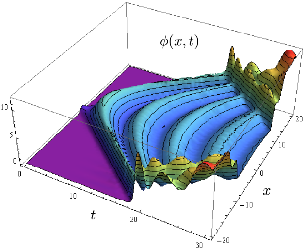
Figure 4: Numerical solution of the SGE (21) in $Mathematica$, with the following data (including the Gaussian initial state, zero initial velocity and symmetric boundary condition): $x\in[-20,20],~{}~{}t\in[0,30],~{}~{}\phi(x,0)=\exp({-x^{2}}),~{}~{}\phi_{t}(x,0)=0,~{}~{}\phi(-20,t)=\phi(20,t)$. Under the same boundary conditions, the SGE with the plus sine gives about 20 times higher amplitude waves, which are all above the zero plane and decrease their width with time. Again, both near-periodicity and nonlinearity of the time evolution are apparent.

The corresponding Hamiltonian densities, of kinetic plus potential energy type, are given in terms of canonically–conjugated coordinate and momentum fields by:

$$\mathcal{H}_{\text{SG}}(\phi,\pi) = \pi\phi_{t}-\mathcal{L}_{\text{SG}}(\phi)=\frac{1}{2}(\pi^{2}+\phi_{x}^{2})+1-\cos\phi,$$

$$\mathcal{H}_{\text{KG}}(\phi,\pi) = \pi\phi_{t}-\mathcal{L}_{\text{KG}}(\phi)=\frac{1}{2}(\pi^{2}+\phi_{x}^{2})+\phi^{2}.$$

Both SGE and KGE are infinite–dimensional Hamiltonian systems [26], with Poisson brackets given by:

$$\left\{F,G\right\}=\int_{-\infty}^{\infty}\left[\frac{\delta F}{\delta\phi(x)}\frac{\delta G}{\delta\pi(x)}-\frac{\delta F}{\delta\pi(x)}\frac{\delta G}{\delta\phi(x)}\right]dx,$$ (8)

so that both (1) and (5) follow from Hamilton’s equations with Hamiltonian $H$ and symplectic form $\omega$:

$$\phi_{t} = \{H,\phi\},\qquad\pi_{t}=\{H,\pi\},\qquad$$

$$\text{{with} \ \ \ }H = \int_{-\infty}^{\infty}\mathcal{H}(\phi,\pi)\,dx,\qquad\omega=\int_{-\infty}^{\infty}d\pi\wedge d\phi\,\,dx.$$ (9)

The Hamiltonian (9) is conserved by the flow of both SGE (1) and KGE (5), with an infinite number of commuting constants of motion (common level sets of these constants of motion are generically infinite-dimensional tori of maximal dimension). Both SGE and KGE admit their own infinite families of conserved functionals in involution with respect to their Poisson bracket (8). This fact allows them both to be solved with the inverse scattering transform (see [11]).

2.2 Momentum and energy of SGE–solitons

SGE is Lorentz–covariant (i.e., invariant with respect to special–relativistic Lorentz transformations; each SGE–soliton behaves as a relativistic object and contracts when $v\rightarrow c\equiv$ the speed of light), and for this fact it has been used in (quantum) field theory. In Minkowski (1+1$\mathbb{)}$ space-time coordinates ($x^{\mu}\in\mathbb{R}^{1,1},\,x^{0}=t,\,x^{1}=x)$ with metric tensor $\eta_{\mu\nu}$ ($\mu,\nu=0,1;\eta_{11}=-\eta_{22}=1,\eta_{11}=\eta_{11}=0$), the SG–Lagrangian density has the following ‘massive form’ of kinetic minus potential energy, with mass $m$ and coupling constant $\lambda$ (see [7]):

$$\mathcal{L}_{\text{SG}}^{\mathrm{Mink}}(\phi)=\frac{1}{2}(\phi_{t}^{2}-\phi_{x}^{2})-\frac{m^{4}}{\lambda}\left[1-\cos\left(\frac{\sqrt{\lambda}}{m}\phi\right)\right]\,,$$

which reduces to the dimensionless form (6) by re-scaling the fields and coordinates:

$$\frac{\sqrt{\lambda}}{m}\phi\rightarrow\phi,\qquad mx^{\mu}\rightarrow x^{\mu}.$$ (12)

The SG–Lagrangian density $\mathcal{L}_{\text{SG}}^{\mathrm{Mink}}(\phi)\equiv\frac{m^{4}}{\lambda}\mathcal{L}_{\text{SG}}(\phi)$ obeys the conservation law and admits topological Noether current [with respect to (12)]:

$$j^{\mu}=\frac{1}{2\pi}\varepsilon^{\mu\nu}\partial_{\nu}\phi\quad\text{with zero-divergence: \ \ }\partial_{\mu}j^{\mu}=0,$$

where $\varepsilon^{\mu\nu}$ is the $\mathbb{R}^{1,1}-$Levi–Civita tensor. The corresponding topological Noether charge is given by:

$$Q = \int\left|\partial_{t}j^{0}(x,t)\right|dx=\frac{1}{2\pi}\left|\phi(+\infty,t)-\phi(-\infty,t)\right|,$$

$$\text{{with} \ }Q_{t} = \frac{1}{2\pi}\left|\phi_{t}(-\infty,t)-\phi_{t}(+\infty,t)\right|=0.$$

The most important physical quality of SGE is its energy–momentum (EM) tensor $T_{\mu\nu}$, which is the Noether current corresponding to spacetime–translation symmetry: $x^{\mu}\rightarrow x^{\mu}+\xi^{\mu};$ this conserved quantity is derived from the Lagrangian (6) as:

$$T_{\mu\nu}=\partial_{\mu}\phi\partial_{\nu}\phi-\eta_{\mu\nu}\mathcal{L}_{\text{SG}}(\phi).$$

$T_{\mu\nu}$ has the following components [7, 31]:

$$T_{00} = \frac{1}{2}(\phi_{t}^{2}+\phi_{x}^{2})+1-\cos\phi,\qquad T_{10}=\phi_{xt}\,=T_{01}.$$

$$T_{11} = \frac{1}{2}(\phi_{t}^{2}+\phi_{x}^{2})-1+\cos\phi,$$

EM’s contravariant form $T^{\mu\nu}$ has the following components:

$$T^{00}=T_{00},\qquad T^{11}=T_{11},\qquad T^{10}=-T_{01}.$$

EM’s conserved quantities are: momentum $P=\int T^{10}dx$, which is the Noether charge with respect to space–translation symmetry, and energy $E=\int T^{00}dx$, which is the Noether charge with respect to time–translation symmetry. Energy and momentum follow from EM’s zero divergence:

$$\partial_{\mu}T^{\mu\nu}=0\Longrightarrow\left\{\begin{array}[]{c}\partial_{t}T^{00}-\partial_{x}T^{10}=0\\ \partial_{t}T^{01}-\partial_{x}T^{11}=0\end{array}\right.\Longrightarrow\left\{\begin{array}[]{c}\partial_{t}E=\partial_{t}\int T^{00}dx=0\\ \partial_{t}P=\partial_{t}\int T^{10}dx=0\end{array}\right..$$

2.3 SGE solutions and integrability

2.3.1 SGE solitons, kinks and breathers

The first 1-soliton solution of the SGE (1) was given by [23, 24] in the form:

$$\phi(x,t)=4\arctan\left[\frac{\sqrt{1-\omega^{2}}\cos(\omega t)}{\omega\cosh(x\sqrt{1-\omega^{2}})}\right],$$

which, for $\omega<1$, is periodic in time $t$ and decays exponentially when moving away from $x=0$.

There is a well-known traveling solitary wave solution with velocity $v$ (see [27]), given by the following generalization of (2):

$$\phi(x,t)=4\arctan\left[\exp\frac{\pm 2(z-z_{0})}{\sqrt{1-v^{2}}\;}\right],\qquad\text{{with} \ \ }\left(z=\mu(x+vt)\right),$$ (13)

and the center at $z_{0}.$ In (13), the case $+2$ describes kink, while the case $-2$ corresponds to antikink.

The stationary kink with the center at $x_{0}$ is defined by:

$$\phi(x)=2\arctan\left[\exp(x-x_{0})\right],$$

(in which the position of the center $x_{0}$ can be varied continuously: $-\infty<x_{0}<\infty$) and represents the solution of the first-order ODE:  $\phi_{x}(x)=\sin\phi(x).$

Regarding solutions of the slightly more general, three-parameter SGE:

$$\phi_{tt}=a\phi_{xx}+b\sin(\lambda\phi),$$ (14)

the following cases were established in the literature (see [10] and references therein):

1. If a function $w=\phi(x,t)$ is a solution of (14), then so are also the following functions:

   $$w_{1} = \frac{2\pi n}{b}\pm\phi(C_{1}\pm x,C_{2}\pm t)\qquad\text{{for} \ \ }\left(n=0,\pm 1,\pm 2,...\right),$$

   $$w_{2} = \pm\phi\left(x\cosh C_{3}+t\sqrt{a}\sinh C_{3},\,\,x\frac{\sinh C_{3}}{\sqrt{a}}+t\cosh C_{3}\right),$$

   where $C_{1}$, $C_{2}$, and $C_{3}$ are arbitrary constants.

2. Traveling-wave solutions:

   $$\phi(x,t) = \frac{4}{\lambda}\arctan\left[\exp\left(\pm\frac{b\lambda(C_{1}x+C_{2}t+C_{3})}{\sqrt{b\lambda(C_{2}^{2}-aC_{1}^{2})}}\right)\right]\quad$$ (15)

   $$\text{{if} \ }b\lambda(C_{2}^{2}-aC_{1}^{2}) > 0,$$

   $$\phi(x,t) = -\frac{\pi}{\lambda}+\frac{4}{\lambda}\arctan\left[\exp\left(\pm\frac{b\lambda(C_{1}x+C_{2}t+C_{3})}{\sqrt{b\lambda(aC_{1}^{2}-C_{2}^{2})}}\right)\right]\quad$$

   $$\text{{if} \ }b\lambda(C_{2}^{2}-aC_{1}^{2}) < 0,$$

   where the first expression (for $b\lambda(C_{2}^{2}-aC_{1}^{2})>0$) represents another 1-soliton solution, which is kink in case of $\ \exp\left(\frac{b\lambda(C_{1}x+C_{2}t+C_{3})}{\sqrt{b\lambda(C_{2}^{2}-aC_{1}^{2})}}\right)$  and antikink in case of $\ \exp\left(-\frac{b\lambda(C_{1}x+C_{2}t+C_{3})}{\sqrt{b\lambda(C_{2}^{2}-aC_{1}^{2})}}\right).$ In case of the standard SGE (1), this kink–antikink expression specializes to the Lorentz-invariant solution similar to (13):

   $$\phi^{\mathrm{K}}(x,t)=4\arctan\left[\exp\left(\frac{\pm(x-x_{c})-vt}{\sqrt{1-v^{2}}}\right)\right],$$ (16)

   where the velocity $v$ ($0<v<1$) and the soliton-center $x_{c}$ are real-valued constants. The kink solution has the following physical (EM) characteristics:

   (i) Energy:

   $$E[\phi^{\mathrm{K}}(x,t)]=\int T^{00}dx=\frac{8}{\sqrt{1-v^{2}}};$$

   (ii) Momentum:

   $$P[\phi^{\mathrm{K}}(x,t)]=\int T^{10}dx=-\frac{8v}{\sqrt{1-v^{2}}}.$$

3. Functional separable solution:

   $$w(x,t)=\frac{4}{\lambda}\arctan\left[f(x)g(t)\right],$$

   where the functions $f=f(x)$ and $g=g(t)$ are determined by the first-order autonomous separable ODEs:

   $$f_{x}^{2}=Af^{4}+Bf^{2}+C,\qquad g_{t}^{2}=-aCg^{4}+(aB+b\lambda)g^{2}-aA,$$

   where $A$, $B$, and $C$ are arbitrary constants. In particular, for $A=0,B=k^{2}>0$, and $C>0$, we have the 2-soliton solution of [28]:

   $$w(x,t)=\frac{4}{\lambda}\arctan\left[\frac{\eta\sin(kx+A_{1})}{k\sqrt{a}\cosh(\eta t+B_{1})}\right],\qquad\text{{with} \ \ }\left(\eta^{2}=ak^{2}+b\lambda>0\right),$$

   where $k$, $A_{1}$, and $B_{1}$ are arbitrary constants.

The only stable traveling wave SGE-solutions for a scalar field $\phi$ are $2\pi$-kinks [40, 41] (localized solutions with identical boundary conditions $\phi=0$ and $\phi=2\pi$). However, easier to follow experimentally are non-localized $\pi$-kinks [43] (separating regions with different values of the field $\phi),$ see also [18] and references therein.

On the other hand, a breather is spatially localized, time periodic, oscillatory SGE–solution (see, e.g. [32]). It represents a field which is periodically oscillating in time and decays exponentially in space as the distance from the center $x=0$ is increased. This oscillatory solution of (1) is characterized by some phase that depends on the breather’s evolution history. This could be, in particular, a bound state of vortex with an antivortex in a Josephson junction. In this case, breather may appear as a result of collision of a fluxon (a propagating magnetic flux-quantum) with an antifluxon, or even in the process of measurements of switching current characteristics. stationary breather solutions form one-parameter families of solutions. An example of a breather–solution of (1) is given by [33]:

$$\phi=4\arctan\left(\frac{\sin T}{u\cosh\left(g(u)x\right)}\right),\qquad$$

with parameters $u=u(t)\$and$\ T=T(t),$ such that

$$g(u)=1/\sqrt{1+u^{2}}\mathrm{\quad and\quad}T(t)=\int_{0}^{t}\,g(u(t^{\prime}))\,u(t^{\prime})\,dt^{\prime}.$$

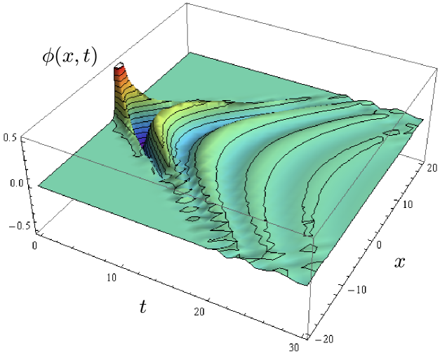
Figure 5: Numerical solution of the damped, unforced SGE (22) in $Mathematica$, with the following data (including the Gaussian initial state, zero initial velocity and symmetric boundary condition): $x\in[-20,20],~{}~{}t\in[0,30],~{}~{}\phi(x,0)=\exp({-x^{2}}),~{}~{}\phi_{t}(x,0)=0,~{}~{}\phi(-20,t)=\phi(20,t),~{}~{}\gamma=0.2,~{}~{}F(x,t)=0$. Damping of the waves is apparent.

2.3.2 Lax–pair and general SGE integrability

In both cases (1) and (3), the SGE admits a Lax–pair formulation:

$$\dot{L}=[L,M],$$ (17)

where overdot means time derivative, $L$ and $M$ are linear differential operators and $[L,M]\equiv LM-ML$ is their commutator (or, Lie bracket).

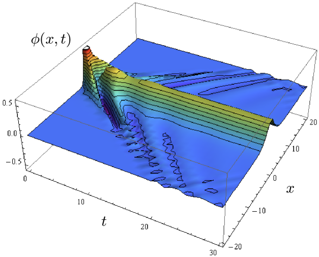
Figure 6: Numerical solution of the damped and spatially-forced SGE (22) in $Mathematica$, with the following data (including the Gaussian initial state, zero initial velocity and symmetric boundary condition): $x\in[-20,20],~{}~{}t\in[0,30],~{}~{}\phi(x,0)=\exp({-x^{2}}),~{}~{}\phi_{t}(x,0)=0,~{}~{}\phi(-20,t)=\phi(20,t),~{}~{}\gamma=0.2,~{}~{}F(x)=0.5\mathop{\mathrm{s}ech}(x)$. We can see the central sech-forcing along all time axis. Damping of the SG-waves is also apparent.

For example, it was shown in [30] that the SGE (1) is integrable through the following Lax pair:

$$\phi_{t}=L\phi,\qquad\phi_{x}=M\phi,\qquad\mathrm{where}$$ (18)

$$L = \left(\begin{array}[]{cc}\frac{\mathrm{i}}{4}(\phi_{x}+\phi_{t})&-\frac{1}{16\lambda}\mathrm{e}^{\mathrm{i}\phi}+\lambda\\ \frac{1}{16\lambda}\mathrm{e}^{-\mathrm{i}\phi}-\lambda&-\frac{\mathrm{i}}{4}(\phi_{x}+\phi_{t})\end{array}\right),\qquad\left(\mathrm{i}=\sqrt{-1}\right)$$

$$M = \left(\begin{array}[]{cc}\frac{\mathrm{i}}{4}(\phi_{x}+\phi_{t})&\frac{1}{16\lambda}\mathrm{e}^{\mathrm{i}\phi}+\lambda\\ -\frac{1}{16\lambda}\mathrm{e}^{-\mathrm{i}\phi}-\lambda&-\frac{\mathrm{i}}{4}(\phi_{x}+\phi_{t})\end{array}\right),\qquad\left(\lambda\in\mathbb{R}\right).$$

The Lax pair (18) possesses the following complex-conjugate symmetry: if $\phi=\left(\begin{array}[]{c}\phi_{1}\\ \phi_{2}\end{array}\right)$ solves the Lax pair (18) at $(\lambda,\phi)$, then $\left(\begin{array}[]{c}\overline{\phi_{2}}\\ \overline{\phi_{1}}\end{array}\right)$ solves the Lax pair (18) at $(-\bar{\lambda},\phi)$. In addition, there is a Darboux transformation for the Lax pair (18) as follows: let

$$u=\phi+2\mathrm{i}\ln\left[\frac{\mathrm{i}\phi_{2}}{\phi_{1}}\right],\qquad\left(u\in\mathbb{R}\right).\qquad$$

If $\phi=\phi|_{\lambda=\nu}$ for some $\nu\in\mathbb{R},$ then

$$\psi=\left(\begin{array}[]{cc}-\nu\phi_{2}/\phi_{1}&\lambda\\ -\lambda&\nu\phi_{1}/\phi_{2}\end{array}\right)\phi.$$

solves the Lax pair (18) at $(\lambda,u)$. Also, from its spatial part: $\phi_{x}=M\phi$, a complete Floquet theory can be developed. See [30] for the proofs and more technical details.

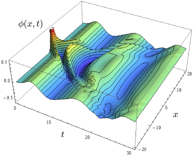
Figure 7: Numerical solution of the damped and temporally-forced SGE (22) in $Mathematica$, with the following data (including the Gaussian initial state, zero initial velocity and symmetric boundary condition): $x\in[-20,20],~{}~{}t\in[0,30],~{}~{}\phi(x,0)=\exp({-x^{2}}),~{}~{}\phi_{t}(x,0)=0,~{}~{}\phi(-20,t)=\phi(20,t),~{}~{}\gamma=0.2,~{}~{}F(x)=0.1\mathop{\mathrm{s}in}(t/2)$. We can see the sine-forcing along all time axis. Damping of the SG-waves is also apparent.

2.4 SGE modifications

2.4.1 SGE with the positive sine term

The simplest SGE modification is to replace the minus sine term with the plus sine:

$$\phi_{tt}=\phi_{xx}+\sin\phi,\qquad\text{{or}}\qquad\phi_{tt}(x,t)=\phi_{xx}(x,t)+\sin\phi(x,t).$$ (21)

Again, a typical, spatially-symmetric, boundary-value problem for (21) is defined by:

$$x \in [-L,L]\subset\mathbb{R},\qquad\left(t\in\mathbb{R}^{+}\right),\hskip 48.36958pt$$

$$\phi(x,0) = f(x),\quad\phi_{t}(x,0)=0,\quad\phi(-L,t)=\phi(L,t),$$

where $f(x)\in\mathbb{R}$ is an axially-symmetric function (see Figure 4).

2.4.2 Perturbed SGE and $\pi$–kinks

As we have seen above (and it was proved by [6, 7]), the (1+1) SGE is integrable. In general though, the perturbations to this equation associated with the external forces and inhomogeneities spoil its integrability and the equation can not be solved exactly. Nevertheless, if the influence of these perturbations is small, the solution can be found perturbatively [33]. The perturbation theory for solitons was developed by [37] and subsequently applied by [38] to dynamics of vortices in Josephson contacts. Perturbed SGEs come in a variety of forms (see, e.g. [37, 38, 39, 42]).

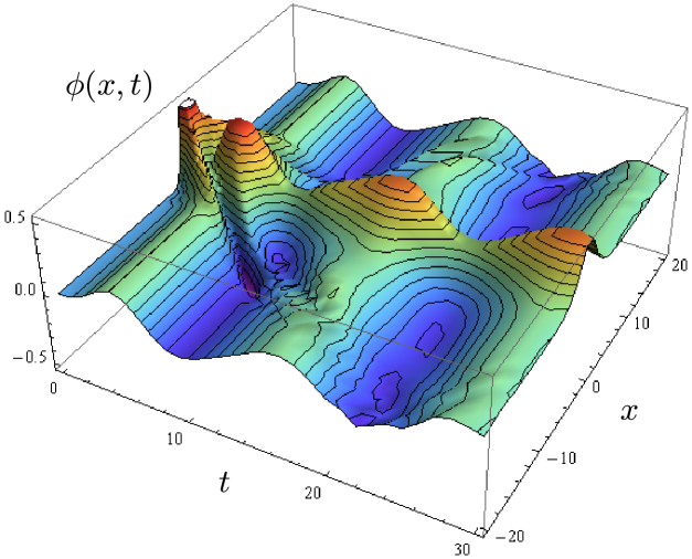
Figure 8: Numerical solution of the damped and both spatially and temporally forced SGE (22) in $Mathematica$, with the following data (including the Gaussian initial state, zero initial velocity and symmetric boundary condition): $x\in[-20,20],~{}~{}t\in[0,30],~{}~{}\phi(x,0)=\exp({-x^{2}}),~{}~{}\phi_{t}(x,0)=0,~{}~{}\phi(-20,t)=\phi(20,t),~{}~{}\gamma=0.2,~{}~{}F(x,t)=0.1\mathop{\mathrm{s}in}(t/2)+0.5\mathop{\mathrm{s}ech}(x)$. We can see both temporal sine-forcing and spatial sech-forcing along all time axis. Damping of the SG-waves is still visible.

One common form is a damped and driven SGE:

$$\phi_{tt}+\gamma\phi_{t}-\phi_{xx}+\sin\phi=F,$$ (22)

where $\gamma\phi_{t}$ is the damping term and $F(x,t)$ is the spatiotemporal forcing. Special cases of the forcing term $F=F(x,t)$ in (22) are: (i) purely temporal $F=F(t)$ (e.g., periodic, see Figure 6); (ii) purely spatial $F=F(x)$ (e.g., central-symmetric, see Figure 7); and (iii) spatiotemporal $F=F(x,t)$ (e.g., temporally-periodic and spatially central-symmetric, see Figure 8).

Considering (for simplicity) purely spatial forcing: $F(x,t)=F(x)$, it has been shown in [47, 48] that if $F(x_{0})=0$ for some point $x_{0}\in\mathbb{R}$, this can be an equilibrium position for the soliton. If there is only one zero, in case of a soliton this is a stable equilibrium position if $\left(\frac{\partial F(x)}{\partial x}\right)_{x_{0}}>0$; in case of an antisoliton, this is a stable equilibrium position if $\left(\frac{\partial F(x)}{\partial x}\right)_{x_{0}}<0$ (see and references therein).

In particular if

$$F(x)=2(\beta^{2}-1)\sinh(\beta x)/\cosh^{2}(\beta x),\qquad(\beta\in\mathbb{R}),$$

the exact stationary kink–solution of (22) is:

$$\phi_{k}=4\arctan\left[\exp\left(\beta x\right)\right].$$

The stability analysis, which considers small amplitude oscillations around
 $\phi_{k}\left[\phi(k,x)=\phi_{k}(x)+f(x)\mathrm{e}^{\lambda t}\right],$ leads to the following eigenvalue problem:

$$\widehat{L}f=\Gamma f,\quad\mathrm{where\quad}\ \widehat{L}=-\partial_{x}^{2}+\left[1-2\cosh^{-2}(\beta x)\right]\quad\mathrm{and\quad}\Gamma=-\lambda^{2}-\gamma\lambda\;.$$

The eigenvalues of the discrete spectrum are given by the formula

$$\Gamma_{n}=\beta^{2}(\Lambda+2\Lambda n-n^{2})-1,$$

where $\Lambda(\Lambda+1)=2/\beta^{2}$. The integer part of $\Lambda$, yields the number of eigenvalues in the discrete spectrum, which correspond to the soliton modes (this includes the translational mode $\Gamma_{0}$, and the internal or shape modes $\Gamma_{n}$ with $n>0$ (see [47, 48]).

In case of a function $F$ defined in such a way that it possesses many zeroes, maxima and minima, perturbed SGE (22) describes an array of inhomogeneities. For example,

$$F(x)={\sum_{n=-q}^{q}4\left(1-\beta^{2}\right)\frac{\mathrm{e}^{\beta\left(x+x_{n}\right)}-\mathrm{e}^{3\beta\left(x+x_{n}\right)}}{\left(\mathrm{e}^{2\beta\left(x+x_{n}\right)}+1\right)^{2}},}$$

where $x_{n}=(n+2)\log\left(\sqrt{2}+1\right)/\beta$ ($n=-q,-q+1\cdots,q-1,q$), and $q+2$ is the number of extrema points of $F(x)$. When the soliton is moving over intervals where $\frac{dF(x)}{dx}<0$, its internal mode can be excited. The points $x_{i}$ where $F(x_{i})=0$ and $\frac{dF(x_{i})}{dx}<0$, are ‘barriers’ which the soliton can overcome due to its kinetic energy (for more details, see [47, 48]).

Study of non-localized $\pi$-kinks in parametrically forced SGE (PSGE):

$$\phi_{tt}\;=\;\phi_{xx}\;-\;a(t/\epsilon)\,\sin\phi,$$ (23)

(over the fast time scale $\epsilon,$ where $a$ is a mean-zero periodic function with a unit amplitude), has been performed by [18, 19], via $2\pi$-kinks as approximate solutions. In particular, a finite-dimensional counterpart of the phenomenon of $\pi$-kinks in PSGE is the stabilization of the inverted Kapitza pendulum by periodic vibration of its suspension point. Geometrical averaging technique of [45] was applied as a series of canonical near-identical transformations via Arnold’s normal form technique [51], as follows.

Starting with the Hamiltonian of PSGE (23), given by:

$$H(\phi)=\int_{-\infty}^{+\infty}\left(\frac{p^{2}}{2}+\frac{\phi_{x}^{2}}{2}-a\cos{\phi}\right)dx,\qquad\mathrm{where}\text{ \ }\left(p\,\equiv\,\phi_{t}\equiv\dot{\phi}\right),$$

a series of canonical transformations was performed in [18] with the aim to kill all rapidly-oscillating terms, the following slightly-perturbed Hamiltonian was obtained:

$$H_{\mathrm{per}}=\int_{-\infty}^{+\infty}\left(\frac{p_{3}^{2}}{2}+\frac{\phi_{3x}^{2}}{2}+\frac{1}{2}\epsilon^{2}\langle a_{-1}^{2}\rangle\sin^{2}{\phi_{3}}\right)dx+O(\epsilon^{3}),$$

which, after rescaling: $X=\epsilon x,\;T=\epsilon t,\;P=2\epsilon^{-1}p_{3},\;\Phi=2\phi_{3},$ gave the following system of a slightly perturbed SGE with $2\pi$-kinks as approximate solutions:

$$\Phi_{T}=P+O(\epsilon^{2}),\qquad P_{T}=\Phi_{XX}-\langle a_{-1}^{2}\rangle\sin{\Phi}+O(\epsilon),$$

where $a_{-1}$ is an anti-derivative with zero average. Finally, after rescaling back to variables $(\phi_{3},p_{3})$, approximate solutions $\phi_{3}\approx\psi(x,t)$ in the form of $\pi$-kinks were obtained, with

$$\psi(x,t)=2\arctan{\left[\exp{\left(\epsilon\sqrt{\langle a_{-1}^{2}\rangle}\frac{x-ct}{\sqrt{1-c^{2}}}\right)}\right]},$$

where $c$ is the wave-propagation velocity. For more technical details, see [18].

In addition, he following two versions of the perturbed SGE have been studied in [19]:

1. Directly forced SGE:

   $$\phi_{tt}-\phi_{xx}+\sin{\phi}=Mf(\omega t).$$

   After shifting to the oscillating reference frame by the transformation:

   $$\phi=\theta+M\omega^{-2}F(\omega t),$$ (24)

   where $F$ has zero mean and $F^{\prime\prime}(\tau)=f(\tau),$ the parametrically forced ODE is obtained:

   $$\ddot{\theta} = -\sin{(\theta+M\omega^{-2}F(\omega t))}\,,\qquad\mathrm{with}$$ (25)

   $$H = \frac{p^{2}}{2}-A(\omega t)\cos(\theta)+B(\omega t)\sin(\theta),$$

   where $p$ is the momentum canonically conjugate to $\theta$, and

   $$A(\omega t)=\cos(M\omega^{-2}F(\omega t)),\qquad B(\omega t)=\sin(M\omega^{-2}F(\omega t)).$$

   From (25), the corresponding evolution PDE (in canonical form) is obtained for a new phase $\theta$ on top of a rapidly oscillating background field:

   $$\theta_{t}=p,\qquad p_{t}=\theta_{xx}-\sin{(\theta+M\omega^{-2}F(\omega t))}.$$

   After retracing the identical transformation (24), the so-obtained (approximate) solutions become $\pi$-kinks (see [19] for technical details).

2. Damped and driven SGE

   $$\phi_{tt}-\phi_{xx}+\sin{\phi}=Mf(\omega t)-\alpha\phi_{t}+\eta,$$ (26)

   which is frequently used to describe long Josephson junctions [38]. Starting with a homogeneous transformation to the oscillating reference frame, analogous to (24) and designed to remove the free oscillatory term: $\phi=\theta+G(t),$ and substituting this transformation to (26), while choosing the function $G$ so that it solves the ODE

   $$\ddot{G}+\alpha\dot{G}=Mf(\omega t),$$

   the following evolution PDE is obtined (in canonical form) [19]:

   $$\theta_{t}=p,\qquad p_{t}=\theta_{xx}-\alpha p+\eta-\sin(\theta+G(\omega t)).$$ (27)

   For the particular case of $f(\tau)=\sin{\tau}$, the the function $G$ is found to be:

   $$G(\tau)=-\frac{\alpha}{\omega}\frac{M}{\alpha^{2}+\omega^{2}}\cos{\tau}-\frac{M}{\alpha^{2}+\omega^{2}}\sin{\tau}.$$

   After a series of transformations (related to a directly-forced pendulum), in zeroth order in $\alpha,\eta$, the evolution PDE (27) reduces (after neglecting terms $\sim\omega^{-3}$) to SGE, which has $\pi$-kink solutions. Therefore, slightly perturbed $\pi$-kinks are approximate solutions of the original equation (26) (on top of the rapidly oscillating background field; see [19] for technical details).

2.4.3 SGE in (2+1) dimensions

The (2+1)D SGE with additional spatial coordinate ($y$) is defined on $\mathbb{R}^{2,1}$as:

$$\varphi_{tt}=\Delta\varphi-\sin\varphi=\varphi_{xx}+\varphi_{yy}-\sin\varphi.$$ (28)

A special class of solutions of (28) can be constructed by generalization of the solution of (1) which does not depend on one of the coordinates, or, obtained by Lorentz transforming the solutions of a stationary 2D SGE. However, there are numerical solutions of (28) which cannot be derived from the (1) or (3), e.g., radial breathers (or, pulsons) [34].

A more general class of solutions of the (2+1)D SG equation has the following form,

$$\varphi(x,y,t)=4\,\arctan\exp\left[y-f(x\pm t)\right],$$ (29)

which exactly satisfies (28) with an arbitrary real-valued twice-differentiable function $f=f(x\pm t)$. The excitations, described by $f$ are similar to elastic shear waves in solid mechanics [46].

Since the equation (28) is Lorentz-covariant, we can obtain other solutions performing Lorentz transformations on (29), which leads to a class of solutions of the form [34]:

$$\varphi(x,y,t)=4\,\arctan\exp\left[\frac{y-v\,t}{\sqrt{1-v^{2}}}-f\left(x\pm\frac{t-v\,y}{\sqrt{1-v^{2}}}\right)\right].$$

2.4.4 Two coupled SGEs

The following two-parameter system of two coupled SGEs was introduced by [49]:

$$\phi_{tt}-\phi_{xx} = -\beta^{2}\sin(\phi-\psi),$$ (30)

$$\psi_{tt}-\alpha^{2}\psi_{xx} = \sin(\phi-\psi),\qquad\text{{with constants} }(\alpha,\beta>0).$$

For numerical solution, see Figure 9.

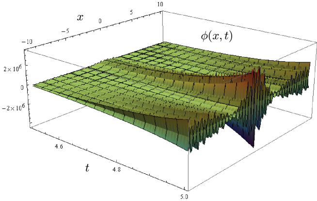
Figure 9: Numerical solution of the SGE-system (30) in $Mathematica$, with the following data:  $x\in[-10,10],~{}~{}t\in[0,5],~{}~{}\alpha=0.5,~{}~{}\beta=0.3,~{}~{}\phi(x,0)=0.3\exp({-x^{2}}),~{}~{}\psi(x,0)=0.7\exp({-x^{2}}),~{}~{}\phi_{t}(x,0)=0,~{}~{}\phi(-10,t)=\phi(10,t),~{}~{}\psi_{t}(x,0)=0,~{}~{}\psi(-10,t)=\psi(10,t)$.

The SGE-system (30) has been exactly solved by [50], where (using a series of substitutions) it was first reduced to the nonlinear second-order ODE:

$$\varphi^{\prime\prime}(\xi)=\left[\frac{1+\alpha^{2}\beta^{2}-c^{2}\left(1+\beta^{2}\right)}{\left(c^{2}-1\right)\left(c^{2}-\alpha^{2}\right)\mu^{2}}+\frac{2\varphi^{\prime 2}}{\varphi(\xi)^{2}+1}\right]\varphi(\xi),$$ (31)

equivalent to the following autonomous system in the $\left(X,Y\right)-$plane:

$$\frac{dX}{d\xi}=Y,\qquad\frac{dY}{d\xi}=\left[\frac{1+\alpha^{2}\beta^{2}-c^{2}\left(1+\beta^{2}\right)}{\left(c^{2}-1\right)\left(c^{2}-\alpha^{2}\right)\mu^{2}}+\frac{2Y^{2}}{X^{2}+1}\right]X.$$ (32)

System (32) has an equilibrium point at the origin: $\left(X,Y\right)=(0,0),$ in which the Jacobian matrix is:

$$J_{(0,0)}=\left(\begin{array}[]{cc}0&1\\ \lambda&0\end{array}\right),\qquad\text{with}\qquad\lambda=\frac{\alpha^{2}\beta^{2}-c^{2}\left(1+\beta^{2}\right)+1}{\left(c^{2}-1\right)\left(c^{2}-\alpha^{2}\right)\mu^{2}}.$$

The phase portraits from this system show that there exist periodic solutions of the coupled SGEs (30).

Using the exponential ansatz:

$$\varphi(\xi)=\frac{p\exp(\xi)+q\exp(-\xi)}{r\exp(\xi)+s\exp(-\xi)},\qquad\text{{with constants} }(p,q,r,s\in\mathbb{R}),$$

four pairs of analytic solutions of the system (31), and therefore of the system (30), were found in [50]. We present here only the first two (simpler) solution pairs:

$$\phi_{1}(x,t) = \frac{\beta^{2}}{4\left(c^{2}-1\right)\mu^{2}}\sin(2\xi)+c_{1}\xi+c2,\quad$$

$$\psi_{1}(x,t) = \frac{\beta^{2}}{4\left(c^{2}-1\right)\mu^{2}}\sin(2\xi)+c_{1}\xi+c2-2\arctan(\tan(\xi)),$$

$$\xi = \mu(x-ct),\,\qquad c=\sqrt{\frac{1-\alpha^{2}\beta^{2}}{1-\beta^{2}}}.$$

$$\phi_{2}(x,t) = \frac{\beta^{2}}{4\left(c^{2}-1\right)\mu^{2}}\sin(2\xi)+c_{1}\xi+c2,\quad$$

$$\psi_{2}(x,t) = \frac{\beta^{2}}{4\left(c^{2}-1\right)\mu^{2}}\sin(2\xi)+c_{1}\xi+c2-2\arctan(\cot(\xi)),$$

$$\xi = \mu(x-ct),\,\qquad c=\sqrt{\frac{1-\alpha^{2}\beta^{2}}{1-\beta^{2}}}.$$

For more technical details, see [50].

2.5 Sine–Gordon chain and discrete breathers

2.5.1 Frenkel–Kontorova model

The original Frenkel–Kontorova model [16, 15, 17] of stationary and moving crystal dislocations, was formulated historically decades before the continuous SGE. It consists of a chain of harmonically coupled atoms in a spatially periodic potential, governed by the set of differential-difference equations:

$$\ddot{\phi}_{n}+\frac{1}{\Delta x^{2}}\left[\phi_{n+1}-2\phi_{n}+\phi_{n-1}\right]+\sin\phi_{n}=0,\,$$ (33)

where $\phi_{n}$ denotes the position of the $n$th atom in the chain. Alternatively, system (33) represents a chain of torsionally-coupled pendula (see Figure 2), where $\phi_{n}$ is the angle which the $n$th pendulum makes with the vertical.

2.5.2 Sine–Gordon chain

To derive dynamical equations of the sine–Gordon chain (SGC), consisting of anharmonic oscillators with the coupling constant $\mu$, we start with the three-point, central, finite-difference approximation of the spatial derivative term $\phi_{xx}$ in the SGE:

$$\phi_{xx} \approx \frac{1}{\Delta x^{2}}\left[\phi_{n+1}-2\phi_{n}+\phi_{n-1}\right]+O(x^{2})$$

$$= -\frac{1}{\Delta x^{2}}\left[(\phi_{n}-\phi_{n-1})-(\phi_{n+1}-\phi_{n})\right]+O(x^{2}).$$

Applying this finite-difference approximation to the SGE (1), and also performing the corresponding replacements: $\phi\rightarrow\phi_{n},~{}\phi_{tt}\rightarrow\ddot{\phi}_{n}$ and $\mu=1/\Delta x^{2},$ we obtain the set of difference ODEs defining the SGC:

$$\ddot{\phi}_{n}+\mu\left[(\phi_{n}-\phi_{n-1})-(\phi_{n+1}-\phi_{n})\right]+\sin\phi_{n}=0\,.$$ (34)

The system (34) describes a chain of interacting particles subjected to a periodic on-site potential $V(x)=\sin(x)$. In the continuum limit, (34) becomes the standard SGE (1) and supports stable propagation of a kink-soliton of the form (16).

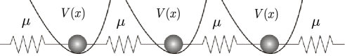
Figure 10: Simple sine–Gordon chain (SGC) with the coupling constant $\mu$ and the periodic on-site potential $V(x)=\sin(x)$.

The linear-wave spectrum of (34) around a kink has either one or two localized modes (which depends on the value of $\mu)$ [35]. The frequencies of these modes lie inside the spectrum gap. The linear spectrum, with the linear frequency $\omega$ and the wave number $k,$ is given by:

$$\omega^{2}=1+4\mu\sin^{2}\frac{k}{2},$$ (35)

while the gap edge frequency is $\omega=1.$

The simplest example of (34), containing only two oscillators, is defined by [35]:

$$\ddot{\phi}_{1,\,2}+\mu(\phi_{1,\,2}-\phi_{2,\,1})+\sin\phi_{1,\,2}=0\,.$$ (36)

It was demonstrated in [44], using the method of averaging in fast oscillations, that a perturbed SGC, damped and driven by a large-amplitude ac-force, might support localized kink solitons. Specifically, they considered the perturbed SGC:

$$\ddot{\phi}_{n}-\mu\left[\phi_{n+1}-2\phi_{n}+\phi_{n-1}\right]+\sin\phi_{n}=\chi+\alpha\sin\omega t-\gamma\dot{\phi}_{n},$$ (37)

where $\chi$ is a dc-force, $\alpha$ and $\omega$ are the normalized (large) amplitude and frequency of a periodic force, respectively, while $\gamma$ is the normalized dissipative coefficient. Without the forcing on the right-hand side, (37) reduces to (34).

2.5.3 Continuum limits

Perturbed SGEs have their corresponding perturbed SGCs. The following $0$-$\pi~{}$SGC was proposed in [52]:

$$\ddot{\phi_{n}}=\frac{\phi_{n-1}-2\phi_{n}+\phi_{n+1}}{a^{2}}-\sin(\phi_{n}+\theta_{n})+\gamma,$$ (38)

as an equation of a phase $\phi_{n}$-motion (of a $0$-$\pi$ array of Josephson junctions). Here, $a$ is the lattice spacing parameter, $\gamma>0$ is the applied bias current density, and $\theta_{n}=(0$ if $n\leq 0$ and $-\pi$ if $n>0)$ is the phase jump of $\pi$ in $\phi_{n}$. The SGC equation (38) is derived from the following discrete Lagrangian:

$$L_{\mathrm{D}}=\int{\sum_{n\in\mathbb{Z}}{\left[\frac{1}{2}\left(\frac{d\phi_{n}}{dt}\right)^{2}-\frac{1}{2}\left(\frac{\phi_{n+1}-\phi_{n}}{a}\right)^{2}-1+\cos(\phi_{n}+\theta_{n})+\gamma\phi_{n}\right]}\,dt}.$$ (39)

In the continuum limit $a\ll 1$ Lagrangian (39) becomes

$$L_{\mathrm{C}}=\iint_{-\infty}^{\infty}\left[\,\frac{1}{2}\left(\phi_{t}\right)^{2}-\frac{1}{2}\left(\widetilde{L}_{a}\phi_{x}\right)^{2}-1+\cos(\phi+\theta)+\gamma\phi\right]\,dx\,dt\,,$$

from which, the continuum limit of (38) gives the following perturbed SGE:

$$\phi_{tt}=L_{a}\phi_{xx}-\sin(\phi+\theta)+\gamma,$$

where $\theta=(0$ if $x\leq 0$ and $-\pi$ if $x>0)$, while the differential operators $L_{a}\phi_{xx}$ and $\widetilde{L}_{a}\phi_{x}$ are given by the following Taylor expansions:

$$L_{a}\phi_{xx} = \frac{\phi_{n-1}-2\phi_{n}+\phi_{n+1}}{a^{2}}=2\sum_{k=0}^{\infty}\frac{a^{2k}}{(2k+2)!}\,\partial_{xx}^{k}\phi_{xx}(na),$$

$$\widetilde{L}_{a}\phi_{x} = \frac{\phi_{n+1}-\phi_{n}}{a}=\sum_{k=0}^{\infty}\frac{a^{k}}{(k+1)!}\,\partial_{x}^{k}\phi(na).$$

For more technical details, including several other continuum limits, see [52].

2.5.4 Discrete breathers

Generally speaking, it is a well-known fact (see, e.g. [58] and references therein) that different types of excitations, most notably phonons (propagating linear waves) and discrete breathers (DBs for short; they are time-periodic spatially localized excitations, also labeled intrinsic localized modes or discrete solitons) can occur as solutions of spatially-discrete nonlinear lattices. According to S. Flach et al. [55, 54, 58] DBs are caused by a specific interplay between the nonlinearity and discreteness of the lattice. The lattice nonlinearity provides with an amplitude-dependent tunability of oscillation or rotation frequencies of DBs, while its spatial discreteness leads to finite upper bounds of the frequency spectrum of small amplitude waves. Although DBs present complex dynamical objects, experimental measurements can (in many cases) be well understood by using their time-averaged properties (see [56]). In addition, nonlinear discrete lattices admit different types of DBs depending on the spectrum of linear waves propagating in the lattice [53, 54, 55, 57], including: acoustic breathers, rotobreathers and optical breathers (see Figure 11).

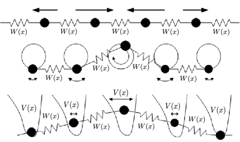
Figure 11: Different types of discrete breathers (DBs): acoustic breather (top), rotobreather (middle), and optical breather (bottom); modified and adapted from [53, 54, 55, 57]).

A particular system studied in [54, 59] has been characterized by the lattice Hamiltonian:

$$H = \sum_{n}(\frac{1}{2}\dot{x}_{n}^{2}+W(x_{n}-x_{n-1})+V(x_{n}))$$

$$= \sum_{n}(\frac{1}{2}p_{n}^{2}+W(x_{n}-x_{n-1})+V(x_{n})),$$

where $x_{n}=x_{n}(t)$ are time-dependent coordinates with canonically-conjugate momenta $p_{n}=\dot{x}_{n}(t),$ $W(x_{n})=W(x)$ is the nearest neighbor interaction, and $V(x_{n})=V(x)$ is an optional on-site (substrate) potential. From (2.5.4) the following equations of motion are derived:

$$\ddot{x}_{n} = -W^{\prime}(x_{n}-x_{n-1})+W^{\prime}(x_{n+1}-x_{n})-V^{\prime}(x_{n}),\qquad\text{{or}}$$

$$\dot{x}_{n} = \dot{x}_{n},\qquad\dot{p}_{n}=-W^{\prime}(x_{n}-x_{n-1})+W^{\prime}(x_{n+1}-x_{n})-V^{\prime}(x_{n}),$$

where (for simplicity) the following zero initial conditions are assumed:

$$V(0)=W(0)=V^{\prime}(0)=W^{\prime}(0)=0,~{}~{}~{}V^{\prime\prime}(0)\geq 0,~{}~{}~{}W^{\prime\prime}(0)>0.$$

Hamiltonian (2.5.4) supports the excitation of small amplitude linear waves:

$$x_{n}(t)\sim\exp\left[\mathrm{i}(\omega_{q}t-qn)\right],$$

with the wave number $q$ and the corresponding frequency spectrum $\omega_{q}^{2}$ which, due to the underlying lattice, depends periodically on $q$:

$$\omega_{q}^{2}=V^{\prime\prime}(0)+4W^{\prime\prime}(0)\sin^{2}\left(\frac{q}{2}\right),$$

and its absolute value has always a finite upper bound. The maximum (Debye) frequency of small amplitude waves is:

$$\omega_{q}=\sqrt{V^{\prime\prime}(0)+4W^{\prime\prime}(0)}.$$

DBs exist for different types of potentials $W(x)$ and $V(x)$. DB solutions are [54] (i) time-periodic: $\hat{x}_{n}(t+T_{b})=\hat{x}_{n}(t),$ and (ii) spatially localized: $\hat{x}_{|n|\rightarrow\infty}\rightarrow 0$. In addition, if the Hamiltonian $H$ is invariant under a finite translation/rotation of any $x_{n}\rightarrow x_{n}+\lambda$, then discrete rotobreathers may exist (see [60]), which are excitations characterized by one or several sites in the breather center evolving in a rotational state: $\hat{x}_{0}(t+T_{b})=\hat{x}_{0}(t)+\lambda$, while outside this center the lattice is governed again by time periodic spatially localized oscillations.

3 Sine–Gordon solitons, kinks and breathers in living cellular structures

In this section, we give the applications of the sine–Gordon equation (and the variety of its traveling–wave solutions), as spatiotemporal models of nonlinear excitations in living cellular structures.

3.1 SGE–solitons in DNA

In this subsection, we review the first three papers describing SGE–solitary excitations in DNA. The first two papers in this domain were published by [62] and [64] – incidentally, under the same title, in the same journal (PRA), using two slightly-different modifications of the same coupled SGE–system (30).

Firstly, Yomosa considered in [62] (see also [63]) the standard Watson–Crick double–helix $B-$form DNA model, in which conformation and stability of DNA and the polynucleotide double helices are determined by:

1. The energy $E_{B}$ of the hydrogen H-bonds between inter-strand complementary base pairs, given by:

   $$E_{B}=\sum_{n}B[1-\cos(\theta_{n}-\theta_{n}^{\prime}-\pi)],$$

   where $B$ is a parameter associated with the H-bond energy, while $\theta_{n}=\measuredangle(B_{n},P_{n})$ and $\theta_{n}^{\prime}=\measuredangle(B_{n}^{\prime},P_{n}^{\prime})$ denote angles between horizontal projections of the complementary base pairs and their corresponding axes;  and

2. The stacking energy $E_{S}$ between intra-strand adjacent bases, given by:

   $$E_{S}=\sum_{n}S[1-\cos(\theta_{n}-\theta_{n-1}-\alpha_{0})]+S[1-\cos(\theta_{n}^{\prime}-\theta_{n-1}^{\prime}-\alpha_{0})],$$

   where $S$ is a parameter associated with the stacking energy of DNA chains and $\alpha_{0}=36^{\circ}.$

Next, by adding the rotational kinetic energy:

$$T_{\mathrm{rot}}=\frac{1}{2}\sum_{n}I[\dot{\theta}_{n}^{2}+\dot{\theta}_{n}^{\prime 2}],$$

(where $I$ is the mean value of the moments of inertia $I_{n}$ of the bases for the rotations around the axes $P$) to the potential energies $E_{B}$ and $E_{S}$, the following SG–chain Hamiltonian for DNA and synthetic polynucleotide double–helices was formulated:

$$H = T_{\mathrm{rot}}+E_{B}+E_{S}=\frac{1}{2}\sum_{n}I[\dot{\theta}_{n}^{2}+\dot{\theta}_{n}^{\prime 2}]+\sum_{n}B[1-\cos(\theta_{n}-\theta_{n}^{\prime}-\pi)]$$ (41)

$$+ \sum_{n}\left\{S[1-\cos(\theta_{n}-\theta_{n-1}-\alpha_{0})]+S[1-\cos(\theta_{n}^{\prime}-\theta_{n-1}^{\prime}-\alpha_{0})]\right\}.$$

From the Hamiltonian (41), via canonical Hamiltonian formalism, the following two sets of coupled SGC–equations of motion were derived in [62]:

$$I\ddot{\theta}_{n}+B\sin(\theta_{n}-\theta_{n}^{\prime}-\pi)+S[\sin(\theta_{n}-\theta_{n-1}-\alpha_{0})-\sin(\theta_{n+1}-\theta_{n}-\alpha_{0})] = 0,$$

$$I\ddot{\theta}_{n}^{\prime}+B\sin(\theta_{n}-\theta_{n}^{\prime}-\pi)+S[\sin(\theta_{n}^{\prime}-\theta_{n-1}^{\prime}-\alpha_{0})-\sin(\theta_{n+1}^{\prime}-\theta_{n}^{\prime}-\alpha_{0})] = 0.$$

Further, by linearizing this coupled ODE-system (assuming the smallness of the angles $\theta_{n}-\theta_{n-1}-\alpha_{0}$ and $\theta_{n}^{\prime}-\theta_{n-1}^{\prime}-\alpha_{0})$ and subsequently performing the continuum limit:

$$\theta_{n}(t)\rightarrow\theta(x,t),\qquad\theta_{n}^{\prime}(t)\rightarrow\theta^{\prime}(x,t),$$ (42)

Yomosa derived the following system of two coupled SGEs, of the (slightly-modified) form of (30):

$$I\theta_{tt}-S\theta_{xx} = -B\sin(\theta-\theta^{\prime}-\pi),$$ (43)

$$I\theta_{tt}^{\prime}-S\theta_{xx}^{\prime} = B\sin(\theta-\theta^{\prime}-\pi).$$

Unfortunately, in his time, Yomosa was not able solve the coupled system (43), so he took the difference of the two SGEs and obtained the following single SGE representing a dynamic (plane) base-rotator model:

$$\frac{1}{v_{0}^{2}}\phi_{tt}=\phi_{xx}-\frac{1}{l^{2}}\sin\phi,\qquad\text{where \ (}v_{0}=\sqrt{\frac{S}{I}},\text{ \ }l=\sqrt{\frac{S}{2B}}).$$ (44)

Finally, by imposing the following boundary condition:

$$\cos\phi = 1\qquad\text{{for} \ }(\phi=2\pi n,\text{ \ \ }n=0,\pm 1,...)\qquad$$

$$\text{{at} \ }\xi = \pm\infty\qquad(\text{{at} \ }x=\pm\infty\quad\text{{for all \ }}t),$$

the following traveling solitary-wave solutions of (44) were obtained in the form (13) of akink–antikink pair:

$$\phi(x,t)=4\,\arctan\exp\left[\pm\frac{\left(\xi-\xi_{0}\right)}{\sqrt{1-v/v_{0}^{2}}l}\right].\text{ \ }$$

Secondly, Zhang clarified in [64] the pioneering (and therefore somewhat-messy) approach of Yomosa and proposed the following modified SGC–Hamiltonian for the $B-$form DNA double–helix (rewritten here in above Yomosa’s notation for consistency):

$$H = \frac{1}{2}\sum_{n}I[\dot{\theta}_{n}^{2}+\dot{\theta}_{n}^{\prime 2}]+\sum_{n}V(\theta_{n},\theta_{n}^{\prime})$$

$$+ \frac{1}{2}\sum_{n}\left[S(\theta_{n}-\theta_{n-1})^{2}+S(\theta_{n}^{\prime}-\theta_{n-1}^{\prime})^{2}\right],$$

where $V(\theta_{n},\theta_{n}^{\prime})$ is the inter-strand interaction energy in $n$th base pair, given by:

$$V(\theta_{n},\theta_{n}^{\prime}) = B[1-\cos(\theta_{n}-\theta_{n}^{\prime})]+\lambda(1-\cos\theta_{n})+\lambda(1-\cos\theta_{n}^{\prime})$$

$$+ \beta\left\{3(1-\cos\theta_{n}\cos\theta_{n}^{\prime})-[1-\cos(\theta_{n}-\theta_{n}^{\prime})]\right\}.$$

From the Hamiltonian (3.1), the following SGC–equations of motion were derived in [64]:

$$I\ddot{\theta}_{n}+B\sin(\theta_{n}-\theta_{n}^{\prime})+\beta[3\sin\theta_{n}\cos\theta_{n}^{\prime}-\sin(\theta_{n}-\theta_{n}^{\prime})]+\lambda\sin\theta_{n}$$

$$\qquad=S(\theta_{n+1}-2\theta_{n}+\theta_{n-1}),$$ (46)

$$I\ddot{\theta}_{n}^{\prime}-B\sin(\theta_{n}-\theta_{n}^{\prime})+\beta[3\cos\theta_{n}\sin\theta_{n}^{\prime}+\sin(\theta_{n}-\theta_{n}^{\prime})]+\lambda\sin\theta_{n}^{\prime}$$

$$\qquad=S(\theta_{n+1}^{\prime}-2\theta_{n}^{\prime}+\theta_{n-1}^{\prime}).$$

By performing the approximation (42), Zhang introduced the continuum variables: $\theta\$and $\theta^{\prime}$. Subsequently, by introducing new variables: $\phi=\theta+\theta^{\prime},$ $\psi=\theta-\theta^{\prime},$ he obtained the following system of two perturbed and coupled SGEs:

$$\phi_{xx}-(1/c_{0}^{2})\phi_{tt} = (1/l^{2})\sin\phi+(2/d^{2})\sin(\phi/2)\cos(\psi/2),$$

$$\psi_{xx}-(1/c_{0}^{2})\psi_{tt} = (1/l^{2})\sin\psi+(2/d^{2})\sin(\psi/2)\cos(\phi/2),$$

$$\text{{where}}\quad c_{0} = \sqrt{S/I},\quad l=\sqrt{S/(3\beta)},\ \quad d=\sqrt{S/\lambda},$$

which cannot be solved analytically. So, by setting $\lambda=0$ in (46), Zhang arrived at the following system of two independent SGEs [(with $Q=(2B+\beta)/(3\beta)$]:

$$\phi_{xx}-(1/c_{0}^{2})\phi_{tt} = (1/l^{2})\sin\phi,$$ (47)

$$\psi_{xx}-(1/c_{0}^{2})\psi_{tt} = (Q/l^{2})\sin\psi,$$

with the simple solution of a single soliton with velocity $c$:

$$\phi_{0}^{\pm}(x,t)=4\,\arctan\exp\left(\pm z\right),\qquad\psi_{0}^{\pm}(x,t)=4\,\arctan\exp\left(\pm\sqrt{Q}\,z\right),$$ (48)

$$\text{{where}}\quad z=(\gamma/l)(\xi-\xi_{0}),\quad\xi=x-ct,\quad\gamma=1/\sqrt{1-c^{2}/c_{0}^{2}}.$$

Finally, by returning to original continuum variables $\theta\$and $\theta^{\prime},$ from (48), Zhang obtained a set of $\pi$-kink/antikink and $2\pi$-kink/antikink solutions (see [64] for more technical details).

The third (and most-cited) paper in this domain (of SGE–solitary excitations in DNA) was [68] (see also [69, 70]), who proposed a discrete SGC model for DNA-promoter dynamics. Salerno introduced the following SGC–Hamiltonian (slightly refined from Yomosa’s and Zhang’s Hamiltonians):

$$H = \frac{1}{2}\sum_{n=1}^{N}I[\dot{\psi}_{n}^{2}+\dot{\theta}_{n}^{2}]+\sum_{n=1}^{N}K\left[(\psi_{n+1}-\psi_{n})^{2}+(\theta_{n+1}-\theta_{n})^{2}\right]$$ (49)

$$+ \sum_{n=1}^{N}\eta_{n}[1-\cos(\psi_{n}-\theta_{n})],$$

where $N$ is the number of base-pairs in the SGC and $K$ is the backbone spring constant along both DNA–helices. $\eta_{n}$ is a nonlinear parameter used to model the strength of H-bonds between complementary bases, chosen according to the following rule: $\eta_{n}=\lambda_{n}\beta$ with $\lambda_{n}=2$ if it refers to $A-T$ or $T-A$ pairs, $\lambda_{n}=3$ otherwise, with $\beta$ a free parameter. From the Hamiltonian (49), the following SGC–equations of motion were derived:

$$I\ddot{\psi}_{n} = K(\psi_{n+1}-2\psi_{n}+\psi_{n-1})-\frac{\beta}{2}\lambda_{n}\sin(\psi_{n}-\theta_{n}),$$ (50)

$$I\ddot{\theta}_{n} = K(\theta_{n+1}-2\theta_{n}+\theta_{n-1})-\frac{\beta}{2}\lambda_{n}\sin(\theta_{n}-\psi_{n}).$$

Further, from (50), the following SGC–equation of motion is obtained for the angle difference: $\phi_{n}=\psi_{n}-\theta_{n}$, between complementary bases:

$$\ddot{\phi}_{n}=\phi_{n+1}-2\phi_{n}+\phi_{n-1}-\frac{\beta}{K}\lambda_{n}\sin\phi_{n}.$$ (51)

We remark that the ODE (51) has the standard form of (34); from it, in the continuum limit, the standard SGE (1) is obtained, with exact soliton solutions (as described in the subsection 2.3.1 before). Salerno used the ODE–model (51) to study nonlinear wave dynamics of the $T7A1-$DNA promoter (see [68] for further technical details).

3.2 SGE–solitons in protein folding

For over a decade, it has been known that nonlinear excitations can influence conformational dynamics of biopolymers; e.g., the effective bending rigidity of a biopolymer chain could lead to a buckling instability [115]. Subsequently, several models have been proposed to explain such protein transition (see, e.g. [116] and references therein).

In this subsection, we review two protein–folding dynamics papers. Firstly, it was suggested in [114] that protein folding may be mediated via interaction of the protein (molecular) chain with SGE–solitons which propagate along the chain. Local potential energy of the chain is modeled by an asymmetric double-well potential:

$$V(\varphi)=\varepsilon(\varphi+\delta)^{2}(\varphi^{2}-{\frac{2}{3}}\varphi\delta+{\frac{1}{3}}\varphi^{2}-2),$$

where the scalar variable $\varphi$ represents local conformation of the protein, $\varepsilon$ is a small positive parameter, while $\delta$ is the asymmetry parameter (ranging from $-1$ to $1)$. The two minima of the potential, corresponding to the local $\alpha$- and $\beta$-conformations of the chain, are positioned at $\varphi=\pm 1$ and the energy-difference between them is:  $\Delta E={\frac{16}{3}}\varepsilon\delta.$

Solitonic excitations are realized in [114] by an additional, dissipative SGE–field $\phi(x),$ where $x$ is the position along the protein. The following interaction potential (with the positive parameter $\Lambda$) is used to mediate interaction between the two fields:

$$u(\phi,\varphi)={\frac{\Lambda}{\Lambda+1}}(1-\cos\phi)\varphi^{2}.$$

The following dissipative equations of motion are derived [114]:

$$\phi_{tt} = \phi_{xx}-{\frac{1+\Lambda\varphi^{2}}{1+\Lambda}}\sin\phi-\gamma_{\phi}\phi_{t},$$ (52)

$$m\varphi_{tt} = -4\varepsilon(\varphi+\delta)(\varphi^{2}-1)-{\frac{2\Lambda}{1+\Lambda}}\varphi(1-\cos\phi)-\gamma_{\varphi}\varphi_{t},$$

where $\gamma_{\phi}\phi_{t}$ and $\gamma_{\varphi}\varphi_{t}$ are dissipative terms. In the small interaction limit (ignoring $\gamma_{\phi}\phi_{t}$), it is chosen:

$$\phi(x,t)=f(x-vt)+\Delta\theta(x,t),\qquad\varphi(x,t)=1+\Delta\varphi(x,t),$$

where $f(z)=4\arctan(\mathrm{e}^{-z})$ is the usual SGE–kink, moving with velocity $v$. For $\varphi(x,t),$ the following approximate sech–soliton solution is obtained:

$$\Delta\varphi\simeq-{\frac{4\Lambda/m}{v^{2}+(\omega/2)^{2}}}\,{\frac{1}{\cosh^{2}(x-vt)}};$$

so, near the center of the $\phi$ kink, $\varphi$ is pushed away from its local minima $\varphi=1$ towards the other local minima. A localized static solution of (52) is found to be:

$$\phi=4\tan^{-1}{\frac{1}{q+\sqrt{1+q^{2}}}},\qquad\varphi^{2}=1-{\frac{\Lambda}{\varepsilon(1+\Lambda)}}\,{\frac{1}{1+q^{2}}},$$

where $q\equiv\sqrt{1-a}\,\sinh(x-x_{0})$, $a=\Lambda^{2}/[2\varepsilon(1+\Lambda)^{2}]{;}$ for more technical details, see [114].

More recently, a Lagrangian field–theory based modeling approach to protein folding has been proposed in [117]. They proposed the protein Lagrangian including three terms:

(i) nonlinear unfolding $\phi^{4}-$protein at the initial state:

$$\mathcal{L}_{\mathrm{unf}}=\frac{1}{2}\left(\partial_{\mu}\phi\right)^{\dagger}\left(\partial^{\mu}\phi\right)+\frac{m_{\phi}^{4}}{\lambda_{\phi}}\left[1-\cos\left(\frac{\sqrt{\lambda_{\phi}}}{m_{\phi}}|\phi|\right)\right];$$

(ii) nonlinear sources injected into the backbone, modeled by $\psi^{4}$ self-interaction:

$$\mathcal{L}_{\mathrm{src}}=\frac{1}{2}\left(\partial_{\mu}\psi\right)^{\dagger}\left(\partial^{\mu}\psi\right)+\frac{\lambda_{\psi}}{4!}\,(\psi^{\dagger}\psi)^{2};$$

(iii) the interaction term (with the coupling constant $\Lambda$):

$$\mathcal{L}_{\mathrm{int}}=-\Lambda\,(\phi^{\dagger}\phi)(\psi^{\dagger}\psi).$$

The total potential (from all three terms) reads:

$$V_{\mathrm{tot}}(\phi,\psi)=\frac{m_{\phi}^{4}}{\lambda_{\phi}}\left[1-\cos\left(\frac{\sqrt{\lambda_{\phi}}}{m_{\phi}}|\phi|\right)\right]+\frac{\lambda_{\psi}}{4!}\,(\psi^{\dagger}\psi)^{2}-\Lambda\,(\phi^{\dagger}\phi)(\psi^{\dagger}\psi).$$

Assuming that $\lambda_{\phi}$is small enough to be approximately at the same order with $\lambda_{\psi}$, the first term can be expanded in term of $\sqrt{\lambda_{\psi}}$, giving (up to the 2^nd order accuracy):

$$V_{\mathrm{tot}}(\phi,\psi)\approx\frac{m_{\phi}^{2}}{2}\,\phi^{\dagger}\phi-\frac{\lambda_{\phi}}{4!}\,(\phi^{\dagger}\phi)^{2}+\frac{\lambda_{\psi}}{4!}\,(\psi^{\dagger}\psi)^{2}-\Lambda\,(\phi^{\dagger}\phi)(\psi^{\dagger}\psi),$$

from which the total Lagrangian: $\mathcal{L}_{\mathrm{tot}}=\mathcal{L}_{\mathrm{unf}}+\mathcal{L}_{\mathrm{src}}+\mathcal{L}_{\mathrm{int}}$ can be (up to the 2^nd-order accuracy) approximated by:

$$\mathcal{L}_{\mathrm{tot}}(\phi,\psi) = \frac{1}{2}\left[\left(\partial_{\mu}\phi\right)^{\dagger}\left(\partial^{\mu}\phi\right)+\left(\partial_{\mu}\psi\right)^{\dagger}\left(\partial^{\mu}\psi\right)\right]$$

$$+\frac{m_{\phi}^{2}}{2}\,\phi^{\dagger}\phi-\frac{\lambda_{\phi}}{4!}\,(\phi^{\dagger}\phi)^{2}+\frac{\lambda_{\psi}}{4!}\,(\psi^{\dagger}\psi)^{2}-\Lambda\,(\phi^{\dagger}\phi)(\psi^{\dagger}\psi).$$

From the Euler–Lagrangian PDEs for the total Lagrangian (3.2):

$$\frac{\partial\mathcal{L}_{\mathrm{tot}}}{\partial|\phi|}-\partial_{\mu}\frac{\partial\mathcal{L}_{\mathrm{tot}}}{\partial(|\partial_{\mu}\phi|)}=0,\;\;\;\;\frac{\partial\mathcal{L}_{\mathrm{tot}}}{\partial|\psi|}-\partial_{\mu}\frac{\partial\mathcal{L}_{\mathrm{tot}}}{\partial(|\partial_{\mu}\psi|)}=0,$$

the following coupled and perturbed SGE and (nonlinear) KGE with cubic forcing are derived:

$$\phi_{tt} = \phi_{xx}-\frac{m_{\phi}^{3}}{\sqrt{\lambda_{\phi}}}\,\sin\left(\frac{\sqrt{\lambda_{\phi}}}{m_{\phi}}|\phi|\right)+2\Lambda\,|\phi||\psi|^{2},$$ (54)

$$\psi_{tt} = \psi_{xx}-\frac{\lambda_{\psi}}{6}\,|\psi|^{3}+2\Lambda\,|\psi||\phi|^{2},$$ (55)

where $\lambda_{\phi}-$ and $\lambda_{\psi}-$terms determine nonlinearities of backbone and source, respectively.

Numerical solution of the two coupled (1+1) PDEs, (54)–(55), with the following boundary conditions:

$$\begin{array}[]{lcl}\phi(0,t)=\phi(L,t)=0\;\;\text{and}\;\;\psi(0,t)=\psi(L,t)=0&\text{for}&0\leq t\leq b,\\ \phi(x,0)=p(x)\;\;\text{and}\;\;\psi(x,0)=f(x)&\text{for}&0\leq x\leq L,\\ \phi_{t}(x,0)=q(x)\;\;\text{and}\;\;\psi_{t}(x,0)=g(x)&\text{for}&0<x<L,\end{array}$$ (56)

(where $p(x)$, $q(x)$, $f(x)$ and $g(x)$ are auxiliary functions), would describe the contour of conformational changes for protein folding. It was performed in [117] using the following forward finite differences:

$$\phi_{i,j+1} = 2\phi_{i,j}-\phi_{i,j-1}+\Delta t^{2}\left(\frac{\phi_{i+1,j}-2\phi_{i,j}+\phi_{i-1,j}}{\Delta x^{2}}+2\Lambda\psi_{i,j}^{2}\phi_{i,j}\right.$$

$$\left.-\frac{m_{\phi}^{3}}{\hbar^{3}\sqrt{\lambda_{\phi}}}\sin\left(\frac{\sqrt{\lambda_{\phi}}}{m_{\phi}}\,\phi_{i,j}\right)\right),$$

$$\psi_{i,j+1} = 2\psi_{i,j}-\psi_{i,j-1}+\Delta t^{2}\left(\frac{\psi_{i+1,j}-2\psi_{i,j}+\psi_{i-1,j}}{\Delta x^{2}}+2\Lambda w_{i,j}^{2}\psi_{i,j}-\frac{\lambda_{\psi}}{6}\psi_{i,j}^{3}\right),$$

where the values at the first time-step $t_{1}$ are given by the boundary conditions (56), while the values at the second time-step $t_{2}$ are determined by the 2^nd-order Taylor expansion:

$$\phi_{i,2} = p_{i}-\Delta tq_{i}+\frac{1}{2}\Delta t^{2}\left(\frac{p_{i+1}-2p_{i}+p_{i-1}}{\Delta x^{2}}+2\Lambda f_{i}^{2}p_{i}\right.$$

$$\left.-\,\frac{m_{\phi}^{3}}{\hbar^{3}\sqrt{\lambda_{\phi}}}\sin\left(\frac{\sqrt{\lambda_{\phi}}}{m_{\phi}}\,p_{i}\right)\right),\qquad(\mathrm{for\ }i=2,3,\cdots,N-1),$$

$$\psi_{i,2} = f_{i}-\Delta tg_{i}+\frac{1}{2}\Delta t^{2}\left(\frac{f_{i+1}-2f_{i}+f_{i-1}}{\Delta x^{2}}+2\Lambda p_{i}^{2}f_{i}-\frac{\lambda_{\psi}}{6}f_{i}^{3}\right).$$

For more technical details, see [117].

3.3 SGE–solitons in microtubules

In this subsection, we review two most-significant papers describing SGE–solitary excitations in microtubules (MTs), and then point-out to some related quantum studies of neural MTs.

3.3.1 Soliton dynamics in MTs

To the best of our knowledge, the first paper describing soliton dynamics in MTs was [72] (see also [73, 74, 75]; for a recent review, see [76]), in which Satarić et al. developed a ferroelectric model of neural MTs where the motion of MT subunits is reduced to a single longitudinal DOF per dimer at a position $n$, denoted by $\phi_{n}.$ The overall effect of the surrounding dimers on a dipole at a chosen site $n$ can be qualitatively described by the following double-well quartic potential:

$$V(\phi_{n})=-\frac{1}{2}A\phi_{n}^{2}+\frac{1}{4}B\phi_{n}^{4}\,,$$ (57)

where $A$ and $B$ are real parameters ($A$ is a linear function of temperature). As an electrical dipole, a dimer in the intrinsic electric field of the MT acquires the additional potential energy given by:

$$V_{\mathrm{el}}=-qE\phi_{n}\,,$$

where $q=18\times 2e$ ($e=$ electron charge) denotes the effective mobile charge of a single dimer and $E$ is the magnitude of the intrinsic electric field. In addition, two more MT–related energies can also be defined:
(i) the potential energy of restoring strain–forces between adjacent dimers in the protofilament (with a unique spring/stiffness constant $k$):

$$V_{\mathrm{str}}=\frac{1}{2}k(\phi_{n+1}-\phi_{n})^{2},\qquad\text{{and}}$$

(ii) the (velocity $\dot{\phi}_{n}-$dependent) kinetic energy associated with the longitudinal displacements of constituent dimers with unique mass $m$:

$$T(\dot{\phi}_{n})=\frac{1}{2}\sum_{n=1}^{N}m\dot{\phi}_{n}^{2},$$

where $N$ is the total number of constituent dimers in the microtubular chain (MTC). The full MTC–Hamiltonian is now given by:

$$H = T(\dot{\phi}_{n})+V_{\mathrm{str}}+V(\phi_{n})+V_{\mathrm{el}}$$

$$= \sum_{n=1}^{N}\left[\frac{1}{2}m\dot{\phi}_{n}^{2}+\frac{1}{2}k(\phi_{n+1}-\phi_{n})^{2}-\frac{1}{2}A\phi_{n}^{2}+\frac{1}{4}B\phi_{n}^{4}\,-qE\phi_{n}\right].$$

Also, in order to derive a realistic equation of motion for the MTC, it is indispensable to include the viscous force: $F_{\mathrm{v}}(\dot{\phi}_{n})=-\gamma\dot{\phi}_{n}$, with the damping coefficient $\gamma.$

Using the Hamiltonian (3.3.1) together with the damping force $F_{\mathrm{v}}(\dot{\phi}_{n}),$ and subsequently performing the continuum limit (with equilibrium spacing $r_{0}$ between adjacent dimers):

$$\phi_{n}(t) \rightarrow \phi(x,t),$$

$$\phi_{n+1}(t) \rightarrow \phi(x,t)+r_{0}\phi_{x}(x,t)+\frac{1}{2}r_{0}^{2}\phi_{xx}(x,t)+...,$$

– Satarić et al. finally derived their nonlinear (forced and damped) wave equation:

$$m\phi_{tt}+\gamma\phi_{t}-kr_{0}^{2}\phi_{xx}=A\phi-B\phi^{3}+qE.$$ (59)

The importance of the electric force term $qE$ lies in the fact that the PDE (59) admits soliton solutions with no energy loss, which acquires the form of a traveling wave, and can be expressed by defining a normalized displacement field [77]:

$$\psi(\xi)=\frac{\phi(\xi)}{\sqrt{A/B}},\quad\text{{with\ \ }}\left(\xi=\alpha(x-vt),\,\alpha=\sqrt{\frac{|A|}{m(v_{0}^{2}-v^{2})}}\right),$$

where $v_{0}=\sqrt{k/m}r_{0}$ is the sound velocity and $v$ is the soliton–propagation velocity. In terms of the $\psi(\xi)$ variable, the wave equation (59) reduces to a damped anharmonic oscillator ODE:

$$\psi^{\prime\prime} + \rho\psi^{\prime 3}+\psi+\sigma=0,\qquad\text{{where}}$$ (60)

$$\rho = \gamma v[m|A|(v_{0}^{2}-v^{2})]^{-\frac{1}{2}},\qquad\sigma=q\sqrt{B}|A|^{-3/2}E,$$

which has a unique bounded solution [72]:

$$\psi(\xi)=a+\frac{b-a}{1+\exp\left(\frac{b-a}{\sqrt{2}}\xi\right)},\qquad\text{{such that:}}$$ (61)

$$(\psi-a)(\psi-b)(\psi-d)=\psi^{3}-\psi-\left(\frac{q\sqrt{B}}{|A|^{3/2}}E\right).$$ (62)

So the kink propagates along the protofilament axis with fixed velocity:

$$v=v_{0}/\sqrt{1+2\gamma^{2}/(9d^{2}m|A|)},$$

which depends on the strength of the electric field $E$ via (62). The total conserved energy of the kink (61) is given by:

$$E = \frac{2\sqrt{2}}{3}\frac{A^{2}}{B}+\frac{\sqrt{2}}{3}k\frac{A}{B}+\frac{1}{2}m^{\ast}v^{2},\qquad\text{{where}}$$ (63)

$$m^{\ast} = \frac{4}{3\sqrt{2}}\frac{mA\alpha}{r_{0}B}\qquad\text{is kink}^{\prime}\text{s \emph{effective} mass.}$$

For the further development of the theory, with kink-antikink waves traveling in opposite directions along the MTC, see [72, 78, 73, 74, 75].

Now, from our general SGE perspective, Satarić model (59) can be approximated by the perturbed SGE (22), rewritten here for our readers’ convenience:

$$\phi_{tt}+\gamma\phi_{t}-\phi_{xx}+\sin\phi=F,$$

– if we apply the following assumptions:
(i) normalized units: $m=k=r_{0}=1$;
(ii) electrical force: $qE=F\equiv F(x,t);$  and
(iii) using the (first two terms of the) Taylor–series expansion of the sine term:

$$\sin\phi=\phi-\frac{1}{6}\phi^{3}+O(\phi^{4})\approx A\phi-B\phi^{3}.$$ (64)

Using assumptions (i)–(ii) and approximation (64), all results of the section 2.4.2 (illustrated with the simulation Figures 4–8) are ready to be employed for the further SGE analysis of solitary excitations in microtubules.

The second paper describing soliton dynamics in MTs was [79]. Under similar assumptions as [72], they proposed the same expresions for the kinetic energy $T(\dot{\phi}_{n})$ and potential energy $V_{\mathrm{str}}$ of restoring strain–forces between adjacent dimers. However, in contrast to the quartic potential (57), Chou et al. followed the recipes from solid state physics [80] and expressed the interaction for the $n$th tubulin molecule of a protofilament by the following periodic (effective) potential:

$$V(\phi_{n})=V_{0}\left[1-\cos\left(\frac{2\pi\phi_{n}}{a_{0}}\right)\right]\,,$$

where $V_{0}$ is the half-height of the potential energy barrier, $\phi_{n}$ is the displacement of the $n$th tubulin molecule within a particular protofilament and $a_{0}=8$nm is the distance between the centers of two neighboring tubulin molecules along a protofilament. In this way, they defined the following MTC–Hamiltonian:

$$H = T(\dot{\phi}_{n})+V_{\mathrm{str}}+V(\phi_{n})$$

$$= \sum_{n=1}^{N}\left[\frac{1}{2}m\dot{\phi}_{n}^{2}+\frac{1}{2}k(\phi_{n+1}-\phi_{n})^{2}+V_{0}\left(1-\cos\frac{2\pi\phi_{n}}{a_{0}}\right)\right].$$

Using canonical Hamilton’s equations, from (3.3.1) they derived the MTC–equations of motion for the $n$th tubulin molecule within a protofilament (for $n=1,2,...N$):

$$m\ddot{\phi}_{n}=k(\phi_{n+1}-2\phi_{n}+\phi_{n-1})-\frac{2\pi V_{0}}{a_{0}}\sin\frac{2\pi\phi_{n}}{a_{0}}.$$ (66)

In the continuum limit: $\phi_{n}(t)\rightarrow\phi(x,t),$ the MTC–equations of motion (66) reduce to the SGE:

$$m\phi_{tt} = ka_{0}^{2}\phi_{xx}-\left(\frac{2\pi}{a_{0}}\right)^{2}V_{0}\sin\phi,\qquad\text{{or}}$$ (67)

$$\phi_{tt} = \frac{1}{c^{2}}\phi_{xx}-\frac{1}{l^{2}}\sin\phi,\qquad\text{{with} \ }\left(c^{2}=\frac{ka_{0}^{2}}{m},~{}~{}\frac{1}{l^{2}}=\frac{4\pi^{2}V_{0}}{ka_{0}^{4}}\right),$$

which is the same SGE as (47) that was used by [64] for DNA–solitons, with kink–antikink solutions (48). Using (67), Chou et al. showed that there was a very high and narrow peak at the center of the kink width, implying that a tubulin molecule would have its maximum momentum when it reaches the top of the periodic potential (for more technical details, see [79]).

In particular, in the case of neural MTs, possibility for sub-neuronal processing of information by cytoskeletal tubulin tails has been proposed by [81], by showing that local electromagnetic field supports information that could be converted into specific protein tubulin-tail conformational states. Long-range collective coherent behavior of the tubulin tails could be modeled in the form of sine-Gordon kinks, antikinks or breathers that propagate along the microtubule outer surface, and the tubulin-tail soliton collisions could serve as elementary computational gates that control cytoskeletal processes. The authors of [81] have used the results of [82], combined with the elastic ribbon SGE–model of [80]. Applying Bäcklund transformations (4) they found 2- and 3-soliton solutions, as well as their elastic collisions. They developed $Maple^{TM}$-based animations of a whole ‘zoo’ of colliding solitons, including kink/antikink pairs and three types of breathers: (i) a standing breather, (ii) a traveling large amplitude breather and (iii) a traveling small amplitude breather.

3.3.2 Liouville’s stringy time–arrow in neural MTs

Now, recall that the term cubic in $\psi$ in the equation of motion (60) was responsible for the appearance of a kink-like classical solution. Let us formulate a Liouville $(1+1)-$string theory of the neural MT–complex, following [78], and consider a general polynomial in $T$ equation of motion for a static tachyon:

$$T^{\prime\prime}(\xi)+\rho T^{\prime}(\xi)=P(T),$$ (68)

(where $\xi$ is some space-like coordinate and $P(T)$ is a polynomial of degree $n)$, in which the ‘friction’ term $T^{\prime}$ expresses a Liouville derivative. In this interpretation of the Liouville field as a local scale on the world-sheet it is natural to assume that the single-derivative term expresses the non-critical string $\beta$-function, and hence is itself a polynomial $R$ of degree $m$: $T^{\prime}(\xi)=R(T)$. Such equations lead to kink-like solutions [83]:

$$T(\xi) = \frac{1}{2a_{4}}\{\mathrm{sgn}(a_{2}a_{4})a_{2}\mathrm{tanh}[\frac{1}{2}a_{2}(x-vt)]-a_{2}\},$$ (69)

$$\text{{where \ }}v = \frac{A_{3}-3a_{2}a_{4}}{a_{4}}\text{ \ {is the velocity,}}$$

which is a universal behavior for biological systems [77], showing the existence of a scheme which admits kink–like solutions for energy transfer without dissipation in cells. The structure of the equation (68), which leads to kink-like solutions (69), is generic for Liouville strings in non-trivial background space-times.

According to the conventional Liouville theorem, written here in terms of Poisson brackets $\{.,.\}$:

$$\rho_{t}=-\{\rho,H\},$$ (70)

the phase-space density of the field theory associated with the matter DOF of the MT–complex evolves with time as a consequence of phase-space volume-preserving symmetries. More generally, statistical description of the temporal evolution of the MT–complex using classical density matrices $\rho(\phi^{i},t)$ [84]:

$$\rho_{t}=-\{\rho,H\}+\beta^{i}G_{ij}\partial_{p_{j}}\rho\,,$$ (71)

where $p_{i}$ are momenta canonically-conjugate to the fields $\phi^{i}$, and $G_{ij}$ is the metric in the space of fields $\{\phi^{i}\}$. The non-Hamiltonian term in (71) leads to a violation of the Liouville theorem (70) in the classical phase space $\{\phi^{i},p_{j}\}$, and constitutes the basis for a dissipative quantum-mechanical description of the system [84], upon density-matrix quantization. In string theory, summation over world sheet surfaces will imply quantum fluctuations of the string target-space background fields $\phi^{i}.$

Using Dirac’s quantization rule:  $\{{.,.}\}\longrightarrow-\mathrm{i}\,[\,{.,.}],$ the quantum version of (71) reads (in terms of the quantum commutator $[{.,.}])$ [84]:

$${\hat{\rho}}_{t}=\mathrm{i}[{\hat{\rho}},{\hat{H}}]+\mathrm{i}\beta^{i}G_{ij}[{\hat{\phi}}^{i},{\hat{\rho}}],$$ (72)

where the hat denotes quantum operators, and appropriate quantum ordering (in the sense of [86]) is understood. In (72), $\hat{H}$ is the Hamiltonian evolution operator, while

$$\hat{\rho}=\sum_{a}P(a)\left|\Psi_{a}\right\rangle\left\langle\Psi_{a}\right|,\quad\text{{with}}\quad(\mathrm{Tr}(\hat{\rho})=1),$$

is von Neumann’s density matrix operator, in which each quantum state $\left|\Psi_{a}\right\rangle$ occurs with probability $P(a)$;  von Neumann’s entropy is defined as:

$$S=-\mathrm{Tr}(\hat{\rho}[\ln\hat{\rho}]).$$

The very structure of the quantum Liouville equation (72) implies the following properties of the MT–complex: [84, 85, 87]:
(i) conservation of probability $P$:

$$P_{t}=\mathrm{Tr}_{t}(\hat{\rho})=0;$$

(ii) conservation of average energy $\left\langle E\right\rangle$:  $\left\langle E\right\rangle_{t}\equiv\mathrm{Tr}_{t}(\hat{\rho}E)=(p_{i}\beta^{i})_{t}=0;$ and
(iii) monotonic increase in entropy $S$:

$$S_{t}\equiv-\mathrm{Tr}_{t}(\hat{\rho}\ln\hat{\rho})=S(\beta^{i}G_{ij}\beta^{j})\geq 0,$$

– which naturally implies a microscopic arrow of time within the MT–complex [87].

3.4 SGE–solitons in neural impulse conduction

Recently, two biophysicists from the Niels Bohr Institute in Copenhahen, T. Heimburg and A. Jackson (see [88, 89]), challenged the half-a-century old electrical theory of neural impulse conduction, proposed by A.L. Hodgkin and A.F. Huxley in the form of their celebrated HH equations (1963 Nobel Prize in Physiology or Medicine). The HH model, which relies on ionic currents through ion channel proteins and the membrane capacitor, is the presently accepted textbook model for the nerve impulse conduction.

For our readers’ reference, here is a brief on the HH model, which (in its basic form) consists of four coupled nonlinear first-order ODEs, including the cable equation for the neural membrane potential $V$, together with $m,h$ and $n$  equations for the gating variables of Na and K channels and leakage (see [92, 93]; for recent reviews, see [94, 95]):

$$C_{m}\dot{V} = -g_{\mathrm{Na}}m^{3}h(V-V_{\mathrm{Na}})-g_{\mathrm{K}}n^{4}(V-V_{\mathrm{K}})-g_{\mathrm{L}}(V-V_{\mathrm{L}})+I_{j}^{\mathrm{ext}},$$

$$\dot{m} = -(a_{m}+b_{m})\,m+a_{m},\qquad\;\dot{h}=-(a_{h}+b_{h})\,h+a_{h},$$ (73)

$$\dot{n} = -(a_{n}+b_{n})\,n+a_{n},\qquad\text{{where}}$$

$$a_{m} = 0.1\,(V+40)/[1-\mathrm{e}^{-(V+40)/10}],\qquad\;b_{m}=4\,\mathrm{e}^{-(V+65)/18},$$

$$a_{n} = 0.01\,(V+55)/[1-\mathrm{e}^{-(V+55)/10}],\qquad b_{n}=0.125\,\mathrm{e}^{-(V+65)/80},$$

$$a_{n} = 0.07\,\mathrm{e}^{-(V+65)/20},\qquad\qquad b_{n}=1/[1+\mathrm{e}^{-(V+35)/10}].$$

Here the reversal potentials of Na, K channels and leakage are: $V_{\mathrm{Na}}=50$ mV, $V_{\mathrm{K}}=-77$ mV and $V_{\mathrm{L}}=-54.5$ mV; the maximum values of corresponding conductivities are: $g_{\mathrm{Na}}=120\;\mathrm{mS/cm}^{2}$, $g_{\mathrm{K}}=36\;\mathrm{mS/cm}^{2}$ and $g_{\mathrm{L}}=0.3\;\mathrm{mS/cm}^{2}$; the capacity of the membrane is: $C_{m}=1\;\mu\mathrm{F/cm}^{2}$. The external, input current is given by:

$$I_{j}^{\mathrm{ext}}=g_{\mathrm{syn}}(V_{a}-V_{c})\sum_{n}\alpha(t-t_{in}),$$ (74)

which is induced by the pre-synaptic spike-train input applied to the neuron $i$, given by:  $U_{i}(t)=V_{a}\sum_{n}\delta(t-t_{in}).$ In (74), $t_{in}$ is the $n$th firing time of the spike-train inputs, $g_{\mathrm{syn}}$ and $V_{c}$ denote the conductance and the reversal potential, respectively, of the synapse, $\tau_{\mathrm{s}}$ is the time constant relevant to the synapse conduction, and $\alpha(t)=(t/\tau_{\mathrm{s}})\;\mathrm{e}^{-t/\tau_{\mathrm{s}}}\Theta(t)\ ($where $\Theta(t)$ is the Heaviside function).

In addition, Hodgkin and Huxley assumed that the total current is the sum of the trans-membrane current and the current along the axon and that a propagating solution exists that fulfills a wave equation, so the simple cable ODE figuring in the basic HH model (73) was further expanded into the following PDE for the propagating nerve impulse depending on the axon radius $a$:

$$\frac{a}{2R_{i}}V_{xx}=C_{m}V_{t}+g_{\mathrm{K}}(V-E_{K})+g_{\mathrm{Na}}(V-E_{Na}),$$

where $R_{i}$ is the resistance of the cytosol within the nerve (see [89] for technical review).

The HH model was originally proposed to account for the property of squid giant axons [92, 93] and it has been generalized with modifications of ion conductances. More generally, the HH–type models have been widely adopted for a study on activities of transducer neurons such as motor and thalamus relay neurons, which transform the amplitude-modulated input to spike-train outputs. For attempts to relate the HH model (as well as its simplified form, Fitzhugh–Nagumo model (FHN) [96, 97]) with propagation of solitons in neural cell membranes see [98] and references therein.

However, the HH model fails to explain a number of features of the propagating nerve pulse, including the reversible release and reabsorption of heat and the accompanying mechanical, fluorescence, and turbidity changes [88, 89]:

“The most striking feature of the isothermal and isentropic compression modulus is its significant undershoot and striking recovery. These features lead generically to the conclusions (i) that there is a minimum velocity of a soliton and (ii) that the soliton profiles are remarkably stable as a function of the soliton velocity. There is a maximum amplitude and a minimum velocity of the solitons that is close to the propagation velocity in myelinated nerves…”

Earlier work of A.V. Hill [91] (another English Nobel laureate), on heat production in nerves (which was based on his previous work on heat production in contracted muscles [90]) is actually reviewed in [93], where it is noted that the heat release and absorption response during the action potential is important ‘but is not understood’.

Based on thermodynamic relation between heat capacity and membrane area compressibility, Heimburg and Jackson considered in [88, 89] a (1+1) hydrodynamic PDE for the dispersive sound propagation in a cylindrical membrane of a density-pulse, governing the changes $\Delta\rho^{A}$ (along the $x$-axis) of the lateral membrane density $\rho^{A}$, defined by: $\Delta\rho^{A}(x,t)=\rho^{A}(x,t)-\rho_{0}^{A}$ , where $\rho_{0}^{A}=4.035\cdot 10^{-3}\,g/m^{2}$ is the equilibrium lateral area density in the fluid phase of the membrane slightly above the melting point. The related sound velocity $c$ can be expanded into a power series (close to the lipid melting transition) as:

$$c^{2}=c_{0}^{2}+p(\Delta\rho^{A})+q(\Delta\rho^{A})^{2}+\ldots,$$ (75)

where $c_{0}=176.6$ m/s is the velocity of small amplitude sound, while $p$ and $q$ are parameters ($p=-16.6\,c_{0}^{2}/\rho_{0}^{A}$ and $q=79.5\,c_{0}^{2}/(\rho_{0}^{A})^{2}$).

In our standard $\phi-$notation, with $\phi(x,t)\equiv\Delta\rho^{A}(x,t)$, the dispersive wave equation of [88, 89] can be written as:

$$\phi_{tt}=c^{2}\phi_{xx}-f(\phi)\,.$$ (76)

Here, we need to make two remarks regarding the dispersive wave equation (76):

1. If the compressibility is approximately constant and if $\Delta\rho^{A}\ll\rho_{0}^{A},$ then the dispersive force $f(\phi)$ is zero and (76) reduces to the standard wave equation (depending only on the small amplitude sound $c_{0}^{2}$):

   $$\phi_{tt}=c_{0}^{2}\phi_{xx}\,.$$

2. If higher sound frequencies (resulting in higher propagation velocities as the isentropic compressibility is a decreasing function of frequency) become dominant, the dispersive forcing function $f(\phi)$ in (76) needs to be defined, or ad-hoc chosen [88, 89] to mimic the linear frequency–dependence of the sound velocity with a positive parameter $h$ as:  $f(\phi)=h\phi_{xxxx\,}.$ In this case, the expansion (75) needs to be explicitely included into PDE (76), resulting in the equation governing dispersive sound propagation, which reads (in original notation of [88, 89]):

   $$\frac{\partial^{2}}{\partial t^{2}}\Delta\rho^{A}=\frac{\partial}{\partial x}\left[\left(c_{0}^{2}+p(\Delta\rho^{A})+q(\Delta\rho^{A})^{2}\right)\frac{\partial}{\partial x}\Delta\rho^{A}\right]-h\frac{\partial^{4}}{\partial x^{4}}\Delta\rho^{A}.$$ (77)

   Furthermore, by introducing the sound propagation velocity $v,$ after the coordinate transformation: $z=x-v\cdot t$, the dispersive PDE (77) can be recast into a time-independent form, describing the shape of a propagating density excitation:

   $$v^{2}\frac{\partial^{2}}{\partial z^{2}}\Delta\rho^{A}=\frac{\partial}{\partial z}\left[\left(c_{0}^{2}+p(\Delta\rho^{A})+q(\Delta\rho^{A})^{2}\right)\frac{\partial}{\partial z}\Delta\rho^{A}\right]-h\frac{\partial^{4}}{\partial z^{4}}\Delta\rho^{A}.$$

   This 1-dimensional PDE has a localized (stationary) solution [99]:

   $$\Delta\rho^{A}(z)=\frac{p}{q}\cdot\frac{1-\left(\frac{v^{2}-v_{min}^{2}}{c_{0}^{2}-v_{min}^{2}}\right)}{1+\left(1+2\sqrt{\frac{v^{2}-v_{min}^{2}}{c_{0}^{2}-v_{min}^{2}}}\cosh\left(\frac{c_{0}}{h}z\sqrt{1-\frac{v^{2}}{c_{0}^{2}}}\right)\right),}$$

   which is a sech-type soliton, a typical solution for KdV and NLS equations.

Now, without arguing either pro- or contra- Heimburg–Jackson theory of neural sound propagation, as an alternative to Hodgkin–Huxley electrical theory, we will simply accept the natural solitary explanation of the nerve impulse conduction, regardless of the physical medium that is carrying it (sound, or heat, or electrical, or smectic liquid crystal [98], or possibly quantum-mechanical [78]). However, we are free to chose a different form for the dispersive force term $f(\phi)$ in the perturbed wave equation (76). For example, instead of the Heimburg–Jackson’s ad-hoc choice of the forth-derivative term, following [72] and subsequent studies of neural MTs, we can choose a double-well quartic dispersive potential (57), which will, combined with the approximation (64), result in the standard SGE (1), generating analytical solutions of the traveling soliton, kink-antikink and breather form (as described in the subsection 2.3.1 before).

3.5 Muscular–contraction solitons on Poisson manifolds

For geometrical analysis of nonlinear PDEs, instead of using common symplectic structures arising in ordinary Hamiltonian mechanics, the more appropriate approach is a Poisson manifold $(\mathbf{g}^{\ast},\,\{F,G\})$, in which $\mathbf{g}^{\ast}$ is a chosen Lie algebra with a $(\pm)$ Lie–Poisson bracket $\{F,G\}_{\pm}(\mu)$) and carries an abstract Poisson evolution equation $\dot{F}\,=\,\{F,H\}$. This approach is well–defined in both the finite– and the infinite–dimensional case (see [110, 111, 112, 113]).

Recall that a Lie algebra consists of a vector (e.g., Banach) space $\mathbf{g}$ carrying a bilinear skew–symmetric operation $[,]:\mathbf{{g}\times{g}\rightarrow{g}}$, called the commutator or Lie bracket. This represents a pairing: $[\xi,\eta]\,=\,\xi\eta\,-\,\eta\xi$  of elements $\xi,\eta\in\mathbf{g}$ and satisfies Jacobi identity:

$$[[\xi,\eta],\mu]+[[\eta,\mu],\xi]+[[\mu,\xi],\eta]=0.$$

Let $\mathbf{g}$ be a (finite– or infinite–dimensional) Lie algebra and $\mathbf{g}^{\ast}$ its dual Lie algebra, that is, the vector space $L^{2}$ paired with $\mathbf{g}$ via the inner product $<,>:\mathbf{g}^{\ast}\times\mathbf{g}\rightarrow\mathbb{R}$. If $\mathbf{g}$ is finite–dimensional, this pairing reduces to the usual action (interior product) of forms on vectors. The standard way of describing any finite–dimensional Lie algebra $\mathbf{g}$ is to provide its $n^{3}$ structural constants $\gamma_{ij}^{k}$, defined by $[\xi_{i},\xi_{j}]\,=\,\gamma_{ij}^{k}\xi_{k}$, in some basis $\xi_{i},\,(i=1,\dots,n)$

For any two smooth functions $F,G:\mathbf{g}^{\ast}\rightarrow\mathbb{R}$, we define the ($\pm$) Lie–Poisson bracket by:

$$\{F,G\}_{\pm}(\mu)=\pm<\mu,\left[{\frac{{\delta F}}{{\delta\mu}}},{\frac{{\delta G}}{{\delta\mu}}}\right]>.$$ (79)

Here $\mu\in\mathbf{g}^{\ast}$, $[\xi,\mu]$ is the Lie bracket in $\mathbf{g}$ and ${{\delta F}/{\delta\mu}}$, ${{\delta G}/{\delta\mu}}\in\mathbf{g}$ are the functional derivatives of $F$ and $G$.

Given a smooth Hamiltonian function $H:\mathbf{g^{\ast}}\rightarrow\mathbb{R}$ on the Poisson manifold $(\mathbf{g}^{\ast},\{F,G\}_{\pm}(\mu))$, the time evolution of any smooth function $F:\mathbf{g^{\ast}}\rightarrow\mathbb{R}$ is given by the abstract Poisson evolution equation:

$$\dot{F}=\{F,H\}.$$ (80)

Now, the basis of Davydov’s molecular model of muscular contraction is oscillations of Amid I peptide groups with associated dipole electric momentum inside a spiral structure of myosin filament molecules (see [101, 102, 103]). There is a simultaneous resonant interaction and strain interaction generating a collective interaction directed along the axis of the spiral. The resonance excitation jumping from one peptide group to another can be represented as an exciton, the local molecule strain caused by the static effect of excitation as a phonon and the resultant collective interaction as a soliton.

Davydov’s own model of muscular solitons was given by the nonlinear Schrödinger equation (NLS) [101, 102]:

$$\mathrm{i}\psi_{t}=-\psi_{xx}+2\chi|\psi|^{2}\psi,$$ (81)

for $-\infty<x<+\infty$. Here $\psi=\psi(x,t)$ is a smooth complex-valued wave function with initial condition $\psi(x,t)|_{t=0}\,=\,\psi(x)$ and $\chi$ is a nonlinear parameter. In the linear limit ($\chi\,=\,0$) (81) becomes the ordinary Schrödinger equation for the wave $\psi$-function of the free 1D particle with mass $m=1/2$ [102].

To put this muscular–contraction model into a rigorous geometrical settings, we can define the infinite-dimensional phase-space manifold $\mathcal{P}=\{(\psi,\bar{\psi})\in S(\mathbb{R}\mathbf{,{C})\}}$, where $S(\mathbb{R}\mathbf{,{C})}$ is the Schwartz space of rapidly-decreasing complex-valued functions defined on $\mathbb{R}$). We define also the algebra $\mathbf{{\chi}(\mathcal{P})}$ of observables on $\mathcal{P}$ consisting of real-analytic functional derivatives ${\delta F}/{\delta\psi}$, ${\delta F}/{\delta\bar{\psi}}\in S(\mathbb{R}\mathbf{,{C})}$. The Hamiltonian function $H:\mathcal{P}\rightarrow\mathbb{R}$ is given by:

$$H(\psi)\,=\,\int_{-\infty}^{+\infty}\left(\left|\psi_{x}\right|^{2}\,+\,\chi|\psi|^{4}\right)dx$$

and is equal to the total energy of the soliton, which is a conserved quantity for (81) (see, e.g. [108, 109]).

The Poisson bracket on $\mathbf{{\chi}(\mathcal{P})}$ represents a direct generalization of the classical finite–dimensional Poisson bracket [104]:

$$\{F,G\}_{+}(\psi)\,=\,\mathrm{i}\int_{-\infty}^{+\infty}\left(\frac{\delta F}{\delta\psi}\frac{\delta G}{\delta\bar{\psi}}\,-\,\frac{\delta F}{\delta\bar{\psi}}\frac{\delta G}{\delta\psi}\right)dx.$$ (82)

It manifestly exhibits skew–symmetry and satisfies Jacobi identity. The functional derivatives are given by:

$${\delta F}/{\delta\psi}\,=\,-\mathrm{i}\{F,\bar{\psi}\}\qquad\mathrm{and\qquad}{\delta F}/{\delta\bar{\psi}}\,=\,\mathrm{i}\{F,\psi\}.$$

Therefore the algebra of observables $\mathbf{{\chi}(\mathcal{P})}$ represents the Lie algebra and the Poisson bracket is the $(+)$ Lie–Poisson bracket $\{F,G\}_{+}(\psi)$. The nonlinear Schrödinger equation (81) for the solitary particle–wave is a Hamiltonian system on the Lie algebra $\mathbf{{\chi}(\mathcal{P})}$ relative to the $(+)$ Lie–Poisson bracket $\{F,G\}_{+}(\psi)$ and Hamiltonian function $H(\psi)$. Therefore the Poisson manifold $(\mathbf{{\chi}(\mathcal{P})}$, $\{F,G\}_{+}(\psi))$ is defined and the abstract Poisson evolution equation (80), rewritten here as: $\ {\dot{\psi}}=\{{\psi},H\},$ which holds for any smooth function ${\psi}:\mathbf{{\chi}(\mathcal{P})\rightarrow}\mathbb{R}$, is equivalent to (81).

An alternative model of muscular soliton dynamics is provided by the Korteweg–deVries equation (KdV, see [104]):

$$f_{t}\,-\,6ff_{x}\,+\,f_{xxx}\,=\,0,\qquad(f_{x}=\partial_{x}f),$$ (83)

where $x\in\mathbb{R}$ and $f$ is a real–valued smooth function defined on $\mathbb{R}$. This equation is related to the ordinary Schrödinger equation by the inverse scattering method (see [108, 109]).

Again, we may define the infinite–dimensional phase–space manifold $\mathcal{V}=\{f\in S(\mathbb{R})\}$, where $S(\mathbb{R}$) is the Schwartz space of rapidly–decreasing real–valued functions $\mathbb{R}$). Further, we define $\mathbf{{\chi}(\mathcal{V})}$ to be the algebra of observables consisting of functional derivatives ${\delta F}/{\delta f}\in S(\mathbb{{R})}$. The Hamiltonian $H:\mathcal{V}\rightarrow\mathbb{R}$ is given by:

$$H(f)\,=\,\int_{-\infty}^{+\infty}(f^{3}\,+\,\frac{1}{2}f_{x}^{2})\,dx,$$

and provides the total energy of the soliton, which is a conserved quantity for (83) (see [108, 109]).

As a real–valued analogue to (82), the $(+)$ Lie–Poisson bracket on $\mathbf{{\chi}(\mathcal{V})}$ is given via (78) by:

$$\{F,G\}_{+}(f)\,=\,\int_{-\infty}^{+\infty}\frac{\delta F}{\delta f}\frac{d}{dx}\frac{\delta G}{\delta f}\,dx.$$

Again it possesses skew–symmetry and satisfies Jacobi identity. The functional derivatives are given by ${\delta F}/{\delta f}\,=\,\{F,f\}$. The KdV equation (83), describing the behavior of the muscular molecular soliton, is a Hamiltonian system on the Lie algebra $\mathbf{{\chi}(\mathcal{V})}$ relative to the $(+)$ Lie–Poisson bracket $\{F,G\}_{+}(f)$ and the Hamiltonian function $H(f)$. Therefore, the Poisson manifold $(\mathbf{\chi}(\mathcal{V}),\{F,G\}_{+}(f))$ is defined and the abstract Poisson evolution equation (80), rewritten here as:  $\dot{f}=\{f,H\},$ which holds for any smooth function $f:\mathbf{{\chi}(\mathcal{V})\rightarrow}\mathbb{R}$, is equivalent to (83).

Another alternative model of muscular soliton dynamics is provided by our SGE (1): $\ \phi_{tt}=\phi_{xx}-\sin\phi$. Again, we may define the infinite–dimensional phase–space manifold $\mathcal{V}=\{\phi\in S(\mathbb{R})\}$, where $S(\mathbb{R}$) is the Schwartz space of rapidly–decreasing real–valued functions $\mathbb{R}$). Further, we define $\mathbf{{\chi}(\mathcal{V})}$ to be the algebra of observables consisting of functional derivatives ${\delta F}/{\delta}\phi\in S(\mathbb{{R})}$. The Hamiltonian $H:\mathcal{V}\rightarrow\mathbb{R}$ is given by:

$$H(\phi)=\int_{-\infty}^{\infty}\left[\frac{1}{2}(\pi^{2}+\phi_{x}^{2})+1-\cos\phi\right]\,dx,$$

and provides the total energy of the soliton, which is a conserved quantity for the SGE (1). The $(+)$ Lie–Poisson bracket on $\mathbf{{\chi}(\mathcal{V})}$ is given via (78) by:

$$\{F,G\}_{+}(\phi)\,=\,\int_{-\infty}^{\infty}\left(\frac{\delta F}{\delta\phi}\frac{\delta G}{\delta\pi}-\frac{\delta F}{\delta\pi}\frac{\delta G}{\delta\phi}\right)dx.$$

Again it possesses skew–symmetry and satisfies Jacobi identity. The functional derivatives are given by: ${\delta F}/{\delta}\phi=\,\{F,\phi\}\in S(\mathbb{{R})}$. The SGE (1), describing the behavior of the molecular muscular soliton, is a Hamiltonian system on the Lie algebra $\mathbf{{\chi}(\mathcal{V})}$ relative to the $(+)$ Lie–Poisson bracket $\{F,G\}_{+}(\phi)$ and the Hamiltonian function $H(\phi)$. Therefore, the Poisson manifold $(\mathbf{\chi}(\mathcal{V}),\{F,G\}_{+}(\phi))$ is defined and the abstract Poisson evolution equation (80), rewritten here as:  $\dot{\phi}=\{\phi,H\},$ which holds for any smooth function $\phi:\mathbf{{\chi}(\mathcal{V})\rightarrow}\mathbb{R}$, is equivalent to (1).

4 Conclusion

In this paper, we have reviewed sine–Gordon equation and its traveling wave solutions. These solitary spatiotemporal processes can serve as realistic models of nonlinear excitations in complex systems in physical sciences as well as in various living cellular structures, including intra–cellular ones (DNA, protein folding and microtubules) and inter–cellular ones (neural impulses and muscular contractions). We have showed that sine–Gordon solitons, kinks and breathers can give us new insights even in such long–time established and Nobel–Prize winning living systems as the Watson–Crick double helix DNA model and the Hodgkin–Huxley neural conduction model.

References

- [1] V.G. Ivancevic, Comment on the review article: Thermostatted kinetic equations as models for complex systems in physics and life sciences, by Carlo Bianca, Physics of Life Reviews 9, 400-402, (2012)
- [2] V.G. Ivancevic, D.J. Reid, Turbulence and Shock-Waves in Crowd Dynamics, Nonlin. Dynamics 68(1-2), 285-304, (2012)
- [3] V.G. Ivancevic, T.T. Ivancevic, Ricci flow and nonlinear reaction-diffusion systems in biology, chemistry, and physics, Nonlin. Dynamics 65(1-2), 35-54, (2011)
- [4] V.G. Ivancevic, T.T. Ivancevic, Complex Nonlinearity: Chaos, Phase Transitions, Topology Change and Path Integrals. Springer, Series: Understanding Complex Systems, Berlin, (2008)
- [5] R.K. Bullough, P.J. Caudrey (Eds.), Solitons, Springer-Verlag, Berlin, (1980)
- [6] M. Ablowitz, H. Segur, Solitons and the Inverse Scattering Transform, SIAM, Philadelphia, (1981)
- [7] R. Rajaraman, Solitons and Instantons. North-Holland, Amsterdam, (1982)
- [8] S.P. Novikov, S.V. Manakov, L.P. Pitaevskii, V.E. Zakharov, Theory of Solitons: The Inverse Scattering Method, Springer-Verlag, (1984)
- [9] A.C. Newell, Solitons in mathematics and physics, SIAM, Philadelphia, (1985)
- [10] A.D. Polyanin, V.F. Zaitsev, Handbook of Nonlinear Partial Differential Equations. Chapman & Hall/CRC Press, (2004)
- [11] L.D. Faddeev, L.A. Takhtajan, Hamiltonian Methods in the Theory of Solitons, Springer, Series: Classics in Mathematics, Berlin, (2007)
- [12] C-L. Terng, K. Uhlenbeck, Geometry of Solitons, Notices of AMS 47, 17-25, (2000)
- [13] B. Meszena, System of Pendulums: A Realization of the Sine-Gordon Model, Wolfram Demonstrations Project, (2013)
- [14] Yu.S. Kivshar, B.A. Malomed, Dynamics of solitons in nearly integrable systems, Rev. Mod. Phys. 61, 763-915, (1989)
- [15] O.M. Braun, Yu.S. Kivshar, Nonlinear dynamics of the Frenkel-Kontorova model, Phys. Rep. 306, 1-108, (1998)
- [16] Y.I. Frenkel, T. Kontorova: J. Phys. Acad. Sci. USSR 1, 137, (1939)
- [17] O.M. Braun, Yu.S. Kivshar, The Frenkel-Kontorova model. Springer Verlag, New York, (2004)
- [18] V. Zharnitsky, I. Mitkov, M. Levi, Parametrically forced sine-Gordon equation and domain walls dynamics in ferromagnets, Phys. Rev. B57(9), 5033, (1998)
- [19] V. Zharnitsky, I. Mitkov, N. Gronbech-Jensen, kinks in strongly ac driven sine-Gordon systems, Phys. Rev. E58(1), R52-R55, (1998)
- [20] Wikipedia, the free encyclopedia, Sine-Gordon equation, (2012)
- [21] Wolfram MathWorld, Sine-Gordon equation, (2012)
- [22] Encyclopedia of Mathematics, L.A. Takhtajan (originator), Sine-Gordon equation, (2012)
- [23] M.J. Ablowitz, D.J. Kaup, A.C. Newell, and H. Segur, Method for solving the sine-Gordon equation. Phys. Rev. Let. 30, 1262-1264, (1973)
- [24] M.J. Ablowitz, P.A. Clarkson, Solitons, nonlinear evolution equations and inverse scattering, Cambridge Univ. Press, Cambridge, (1991)
- [25] G. Darboux, Lecon sur la théorie générale des surfaces (3rd ed.). Chelsea, (1972)
- [26] R. Temam, Infinite Dimensional Dynamical Systems in Mechanics and Physics (2nd ed.), Springer-Verlag, NY, (1996)
- [27] M. Tabor, Chaos and integrability in nonlinear dynamics, John Wily & Sons, NY, (1989)
- [28] J.K. Perring, T.H.R. Skyrme, A Model Unified Field Equation. Nucl. Phys. 31, 550-555, (1962)
- [29] P. Lax, Integrals of nonlinear equations of evolution and solitary waves, Comm. Pure App. Math. 21(5), 467-490, (1968)
- [30] Y.C. Li, Homoclinic tubes and chaos in perturbed sine-Gordon equation, Chaos, Solitons & Fractals 20(4), 791-798, (2004)
- [31] J.M. Guilarte, Lectures on quantum sine-Gordon models, Univ. Fed. Matto Grosso, Brazil, (2010)
- [32] M. Haskins, J.M. Speight, Nonlinearity 11, 1651-1671, (1998)
- [33] D.R. Gulevich, F.V. Kusmartsev, Perturbation theory for localized solutions of sine-Gordon equation: decay of a breather and pinning by microresistor, Phys. Rev. B74, 214303, (2006)
- [34] D.R. Gulevich, F.V. Kusmartsev, S. Savel’ev, V.A. Yampol’skii, F. Nori, Shape waves in 2D Josephson junctions: exact solutions and time dilation, Phys. Rev. Lett. 101, 127002, (2008)
- [35] J.E. Prilepsky, A.S. Kovalev, On the internal modes in sine-Gordon chain, Phys. Rev. E71, 046601, (2005)
- [36] B. Bodo, S. Morfu, P. Marquié, B.Z. Essimbi, Noise induced breather generation in a sine-Gordon chain, J. Stat. Mech. The. Exp. 01, 01026, 8 pp. (2009)
- [37] J.P. Keener, D.W. McLaughlin, Solitons under perturbations, Phys. Rev. A16, 777-790, (1977)
- [38] D.W. McLaughlin, A.C. Scott, Perturbation analysis of fluxon dynamics, Phys. Rev. A18, 1652-1680, (1978)
- [39] D.J. Kaup, A.C. Newell, Theory of Nonlinear Oscillating Dipolar Excitations in One-Dimensional Condensates, Phys. Rev. B18, 5162-5167, (1978)
- [40] O.H. Olsen, M.R. Samuelsen, Sine-Gordon 2-kink dynamics in the presence of small perturbations, Phys. Rev. B28(1), 210-217, (1983)
- [41] P.C. Dash, Correct dynamics of sine-Gordon 2-kink in presence of periodic perturbing force, J. Phys. C: Solid State Phys. 18, L125, (1985)
- [42] D.J. Kaup, Perturbation theory for solitons in optical fibers, Phys. Rev. A42, 5689-5694, (1990)
- [43] Yu.S. Kivshar, N. Gronbech-Jensen, M.R. Samuelsen, Pi kinks in a parametrically driven sine-Gordon chain, Phys. Rev. B45(14), 7789-7794, (1992)
- [44] N. Gronbech-Jensen, Yu. S. Kivshar, Inverted kinks in ac driven damped sine-Gordon chains, Phys. Let. A171, 338-343, (1992)
- [45] M. Levi, Geometry and physics of averaging with applications, Physica D132, (1-2), 150-164, (1999)
- [46] Y.C. Fung, Foundations of Solid Mechanics, Prentice Hall, New Jersey, (1965)
- [47] J.A. Gonzalez, A. Bellorin, L.E. Guerrero, Internal modes of sine-Gordon solitons in the presence of spatiotemporal perturbations, Phys. Rev. E65, 065601(R), (2002)
- [48] J.A. Gonzalez, A. Bellorin, L.E. Guerrero, How to excite the internal modes of sine-Gordon solitons, Cha. Sol. Fra. 17, 907, (2003)
- [49] K.R. Khusnutdinova, D.E. Pelinovsky, On the exchange of energy in coupled Klein Gordon equations, Wave Motion 38, 1-10, (2003)
- [50] A.H. Salas, Exact solutions of coupled sine-Gordon equations, Nonl. Anal. Real World Appl. 11, 3930 3935, (2010)
- [51] V.I. Arnold, Geometrical methods in the theory of ordinary differential equations, Springer-Verlag, (1983)
- [52] G. Derks, A. Doelman, S.A. van Gils, H. Susanto, Stability analysis of -kinks in a 0- Josephson junction, SIAM J. Appl. Dyn. Syst. 6, 99-141, (2007)
- [53] S. Aubry, Breathers in nonlinear lattices: Existence, linear stability and quantization (Lattice dynamics, Paris, 1995); Physica D103, 201-250, (1997)
- [54] S. Flach, A.E. Miroshnichenko, M.V. Fistul, Wave scattering by discrete breathers, Chaos 13, 596-609, (2003)
- [55] S. Flach, C.R. Willis, Discrete breathers, Phys. Rep. 295, 182-264, (1998)
- [56] A.E. Miroshnichenko, S. Flach, M.V. Fistul, Y. Zolotaryuk, J.B. Page, Breathers in Josephson junction ladders: Resonances and electromagnetic wave spectroscopy, Phys. Rev. E64, 066601, (2001)
- [57] S. Flach, A.V.Gorbach, Discrete breathers in Fermi-Pasta-Ulam lattices, Chaos 15, 015112, (2005)
- [58] S. Flach, A.V.Gorbach, Discrete breathers - Advances in theory and applications, Phys. Rep. 467, 1-116, (2008)
- [59] S. Flach, A.V.Gorbach, Discrete breathers with Dissipation, A Chapter in Dissipative Solitons: From Optics to Biology and Medicine (Eds. A. Ankiewicz, N. Akhmediev), Springer: Lect. Notes in Physics 751, 1-32, (2008)
- [60] S. Takeno, M. Peyrard, Nonlinear modes in coupled rotator models, Physica D92, 140, (1996)
- [61] S.W. Englander, N.R. Kallenbach, A.J. Heeger, J.A. Krumhansl, S. Litwin, Nature of the open state in long polynucleotide double helices: possibility of soliton excitations, Proc. Natl. Acad. Sci. U.S.A. 77(12), 7222-7226, (1980)
- [62] S. Yomosa, Soliton excitations in deoxyribonucleic acid (DNA) double helices, Phys. Rev. A27, 2120-2125, (1983)
- [63] S. Yomosa, Solitary excitations in deoxyribonuclei acid (DNA) double helices, Phys. Rev. A30, 474-480, (1984)
- [64] C-T. Zhang, Soliton excitations in deoxyribonucleic acid (DNA) double helices, Phys. Rev. A35(2), 886-891, (1987)
- [65] J.A. Pople, Molecular association in liquids II. A theory of the structure of water. Proc. Roy. Soc. London A205, 163-178, (1951)
- [66] L.V. Yakushevich, The effects of damping, external fields and inhomogeneity on the nonlinear dynamics of biopolymers, Stud. Biophys. 121, 201, (1987)
- [67] L.V. Yakushevich, Nonlinear physics of DNA (2nd ed.), John Wiley & Sons, (2006)
- [68] M. Salerno, Discrete model for DNA-promoter dynamics, Phys. Rev. A44(8), 5292-5297, (1991)
- [69] M. Salerno, Dynamical Properties of DNA Promoters, Phys. Lett. A167, 49-53 (1992)
- [70] M. Salerno, Yu. Kivshar, DNA promoters and nonlinear dynamics, Phys. Lett. A193, 263-266, (1994)
- [71] P. Dustin, Microtubules, Springer, Berlin, (1984)
- [72] M.V. Satarić, J.A. Tuszyńsky, R.B. Žakula, Kinklike excitations as an energy-transfer mechanism in microtubules. Phys. Rev. E48, 589-597, (1993)
- [73] M.V. Satarić, S. Zeković, J.A. Tuszyńsky, J. Pokorni, Mossbauer effect as a possible tool in detecting nonlinear excitations in microtubules. Phys. Rev. E58, 6333-6339, (1998)
- [74] M.V. Satarić, J.A. Tuszyńsky, Relationship between ferroelectric liquid crystal and nonlinear dynamics of microtubules. Phys. Rev. E67, 011901-011911, (2003)
- [75] S. Zdravković, L. Kavitha, M.V. Satarić, S. Zeković, J. Petrović, Modified extended tanh-function method and nonlinear dynamics of microtubules, Chaos, Solitons & Fractals 45(11), 1378-1386, (2012)
- [76] V.G. Ivancevic, T.T. Ivancevic, Quantum Neural Computation, Springer, Series: Intelligent Systems, Control and Automation, (2009)
- [77] P. Lal, Kink solitons and friction, Phys. Lett. A111, 389, (1985)
- [78] N.E. Mavromatos, D.V. Nanopoulos, A Non-Critical String (Liouville) Approach to Brain Microtubules: State Vector Reduction, Memory Coding and Capacity, Int. J. Mod. Phys. B11, 851, (1997)
- [79] K.C. Chou, C.T. Zhang, G.M. Maggiora, Solitary wave dynamics as a mechanism for explaining the internal motion during microtubule growth, Biopolymers, 34(1), 143-53, (1994)
- [80] R.K. Dodd, J.C. Eilbeck, J.D. Gibbon, H.C. Morris, Solitons and Nonlinear Wave Equations, Academic Press, London, (1982)
- [81] D.D. Georgiev, S.N. Papaioanou, J.F. Glazebrook, Solitonic effects of the local electromagnetic field on neuronal microtubules, Neuroquantology 5(3), 276-291, (2007)
- [82] E. Abdalla, B. Maroufi, B.C. Melgar, M.B. Sedra, Information transport by sine-Gordon solitons in microtubules, Physica A301, 169-173, (2001)
- [83] M. Otwinowski, R. Paul, W. Laidlaw, Exact travelling wave solutions of a class of nonlinear diffusion equations by reduction to a quadrature, Phys. Lett. A128, 483, (1988)
- [84] J. Ellis, N.E. Mavromatos, D.V. Nanopoulos, String theory modifies quantum mechanics, Phys. Lett. B293, 37-48, (1992)
- [85] J. Ellis, N.E. Mavromatos, D.V. Nanopoulos, How large are dissipative effects in non-critical Liouville string theory? Phys. Rev. D63, 024024, (2001)
- [86] G. Lindblad, On the generators of quantum dynamical semigroups, Comm. Math. Phys. 48, 119-130, (1976)
- [87] D.V. Nanopoulos, As time goes by, Riv. Nuovo Cim. 17N10, 1-53, (1994)
- [88] T. Heimburg, A.D. Jackson, On soliton propagation in biomembranes and nerves, Proc. Natl. Acad. Sci. USA, 102(28), 9790-9795, (2005)
- [89] T. Heimburg, A.D. Jackson, On the action potential as a propagating density pulse and the role of anesthetics, Biophys. Rev. Let. 2, 57-78, (2007)
- [90] A.V. Hill, The heat of shortening and the dynamic constants of muscle, Proc. R. Soc. London B76, 136-195, (1938)
- [91] B.C. Abbott, A.V. Hill, J.V. Howarth, The positive and negative heat production associated with a nerve impulse, Proc. R. Soc. London B148(931), 149-87, (1958)
- [92] A.L. Hodgkin, A.F. Huxley, A quantitative description of membrane current and application to conduction and excitation in nerve, J. Physiol. (London) 117, 500-544, (1952)
- [93] A.L. Hodgkin, The Conduction of the Nervous Impulse, Liverpool Univ. Press, (1964)
- [94] D. Guo, Q. Wang, M. Perc, Complex synchronous behavior in interneuronal networks with delayed inhibitory and fast electrical synapses, Phys. Rev. E85, 061905, (2012)
- [95] T. Ivancevic, H. Greenberg, R. Greenberg, Sport Without Injuries And Ultimate Health through Nature, Science and Technology, Springer, Series: Cognitive Systems Monographs, Berlin, (in press)
- [96] R. FitzHugh, Mathematical models of threshold phenomena in the nerve membrane, Bull. Math. Biophys. 17, 257-269, (1955)
- [97] J. Nagumo, S. Arimoto, S. Yoshizawa, An active pulse transmission line simulating nerve axon. Proc. IRE 50, 2061-2070, (1962)
- [98] P. Das, W.H. Schwarz, Solitons in cell membranes, Phys. Rev. E51, 3588-3612 (1995)
- [99] B. Lautrup, R. Appali, A.D. Jackson, T. Heimburg, The stability of solitons in biomembranes and nerves, Eur. Phys. J.E. Soft Matter 34(6), 1-9, (2011)
- [100] V.G. Ivancevic, T.T. Ivancevic, Natural Biodynamics. World Scientific, Series: Mathematical Biology, Singapore, (2006)
- [101] A.S. Davydov, The theory of contraction of proteins under their excitation. J. Theor. Biol. 38, 559-569, (1973)
- [102] A.S. Davydov, Biology and Quantum Mechanics, Pergamon Press, New York, (1982)
- [103] A.S. Davydov, Solitons in Molecular Systems. (2nd ed), Kluwer, Dordrecht, (1991)
- [104] V. Ivancevic, C.E.M. Pearce, Poisson manifolds in generalised Hamiltonian biomechanics. Bull. Austral. Math. Soc. 64, 515-526, (2001)
- [105] V.G. Ivancevic, Nonlinear complexity of human biodynamics engine, Nonlin. Dynamics 61(1-2), 123-139, (2010)
- [106] V.G. Ivancevic, Adaptive-Wave Alternative for the Black-Scholes Option Pricing Model, Cogn. Comput, 2(1), 17-30, (2010)
- [107] V.G. Ivancevic, Adaptive wave models for sophisticated option pricing, J. Math. Finance 1, 41-49, (2011)
- [108] W.M. Seiler, R.W. Tucker, Involution and constrained dynamics I: The Dirac approach, J. Phys. A28, 4431-4451, (1995)
- [109] W.M. Seiler, Involution and constrained dynamics II: The Faddeev-Jackiw approach, J. Phys. A28, 7315-7331, (1995)
- [110] J.E. Marsden, T.S. Ratiu, Introduction to Mechanics and Symmetry: A Basic Exposition of Classical Mechanical Systems (2nd ed), Springer, New York, (1999)
- [111] V.G. Ivancevic, T.T. Ivancevic, Geometrical Dynamics of Complex Systems: A Unified Modelling Approach to Physics Control Biomechanics Neurodynamics and Psycho-Socio-Economical Dynamics. Springer, Dordrecht, (2006)
- [112] V.G. Ivancevic, T.T. Ivancevic, Applied Differential Geometry: A Modern Introduction. World Scientific, Series: Mathematics, Singapore, (2007)
- [113] V.G. Ivancevic, T.T. Ivancevic, New Trends in Control Theory, World Scientific, Series: Stability, Vibration and Control of Systems, Singapore, (2012)
- [114] S. Caspi, E. Ben-Jacob, Toy Model Studies of Soliton Mediated Protein Folding and Conformation Changes, Europhys. Let. 47, 522-527, (1999)
- [115] S.F. Mingaleev, Y.B. Gaididei, P.L. Christiansen, Y. Kivshar, Nonlinearity-induced conformational instability and dynamics of biopolymers, Europhys. Lett. 59, 403-409, (2002)
- [116] A. Sulaiman, F.P. Zen, H. Alatas, L.T. Handoko, Anharmonic oscillation effect on the Davydov-Scott monomer in a thermal bath, Phys. Rev. E81, 061907, (2010)
- [117] M. Januar, A. Sulaiman, L.T. Handoko, Nonlinear conformation of secondary protein folding, Int. J. Mod. Phys. Conf. Ser. 9, 127-132, (2012)