Using spherical wavelets to search for magnetically-induced alignment in the arrival directions of ultra-high energy cosmic rays

Abstract

Due to the action of the intervening cosmic magnetic fields, ultra-high energy cosmic rays (UHECRs) can be deflected in such a way as to create clustered energy-ordered filamentary structures in the arrival direction of these particles, the so-called multiplets. In this work we propose a new method based on the spherical wavelet transform to identify multiplets in sky maps containing arrival directions of UHECRs. The method is illustrated in simulations with a multiplet embedded in isotropic backgrounds with different numbers of events. The efficiency of the algorithm is assessed through the calculation of Type I and II errors.

1 Introduction

Cosmic rays were discovered more than one century ago. One remarkable feature of the cosmic ray spectrum is that it spans more than ten orders of magnitude, up to hundreds of EeV (1 EeV $=10^{18}$ eV). The spectrum roughly follows an inverse power law, which means that the expected flux of particles at the highest energies is extremely low compared to the lower energies. In fact, at energies of a few EeV, only one particle per square kilometer per year is expected. Particles with energies $\gtrsim$ 1 EeV are referred to as ultra-high energy cosmic rays. Some experiments, such as the Pierre Auger Observatory and the Telescope Array Project, have been designed to increase the statistics of events in this energy range. Despite the improved statistics, questions pertaining to the origin, nature and mechanisms of acceleration of these particles, remain unanswered.

Due to the presence of galactic and extragalactic magnetic fields, charged cosmic rays are expected to be deflected. Hence, incoming directions, as measured by a detector, do not point back to the exact position of the source. The magnitude of the deflection depends on the strength of the intervening fields. In the case of charged particles the deflections are roughly inversely proportional to the particle energy. Therefore, for coherent fields, the different Larmor radii described by cosmic rays can create filamentary structures ordered by energy, known as multiplets. This allows the reconstruction of the source position, and consequently enhances the possibility to do astronomy with UHECRs.

In this paper we propose a new method of identifying multiplets, based on the spherical wavelet transform. The paper is organized as follows: in section 2, we review the physics underlying multiplets; in section 3 we present the wavelet transform from a pattern matching algorithm point of view, and give motivations for its use in cosmic ray physics; in section 4 we present a novel algorithm to identify filamentary structures in cosmic ray maps; in section 5 the method is applied to simulated data sets; in section 6, we present our results; in section 7 we make our final remarks.

2 Cosmic Magnetic Fields and Multiplets

Several results show that at ultra-high energies the cosmic ray spectrum contains atomic nuclei. Data from the High Resolutions Fly’s Eye Experiment (HiRes) indicate that UHECRs are probably protons [1], whereas the results from the Pierre Auger Observatory indicate that the composition tends to heavy nuclei at the highest energies [2]. Despite this controversy, one can consider that UHECRs are predominantly charged particles and, as such, can be deflected by magnetic fields.

The deflection expected for a UHECR of charge $Z$ due to the regular component of the galactic magnetic field (GMF) is given approximately by [3]:

$$\delta\approx 53^{\circ}\frac{Z}{E}\left|\int\limits_{0}^{L}\frac{d\vec{r}}{\mbox{kpc}}\times\frac{\vec{B}}{\mbox{$\mu$G}}\right|{\ }\mbox{EeV},$$ (1)

where $E$ is the energy of the particle, $\vec{B}$ the magnetic field, and $L$ the travel distance of the particle. Since $|\vec{B}|\sim\mu$G and is coherent over lengths of $\sim$ 10 kpc, typical deflections are $\sim$ 10^∘ for protons of 10 EeV.

The expected deflection due to the turbulent component is [4]:

$$\delta_{turb}\approx 10^{\circ}\frac{Z{\ }{\mbox{EeV}}}{E}\frac{B_{rms}}{\mbox{$\mu$G}}\sqrt{\frac{L}{\mbox{kpc}}}\sqrt{\frac{L_{c}}{\mbox{50 pc}}},$$ (2)

where $B_{rms}$ is the root mean square intensity of the magnetic field and $L_{c}$ is its coherence length.

According to equation (1) the deflection is inversely proportional to the energy of the particle. Therefore it is possible that energy ordered filamentary structures, the so-called multiplets, can be detected in cosmic ray maps as shown in figure 1. Another method to detect filamentary structures in the arrival directions distributions of UHECRs was proposed by Harari et al.[5].

An interesting property of the multiplets is that the position of the source can be reconstructed, allowing one to identify UHECRs sources. A method to reconstruct the source position of a multiplet was presented by Golup et al. [6] and was used by the Pierre Auger Collaboration to estimate the position of the sources for some possible multiplet candidates [4]. In the aforementioned work, no statistically significant evidence for multiplets arising from magnetic deflections was found for energies above 20 EeV.

Figure 1: Illustration of a multiplet on the tangent plane of a sky map. The dots represent events from higher (red) to lower (blue) energies. The black dot corresponds to the position of the source.

It is important to notice that for some models of the galactic magnetic fields such as the ones proposed by [7, 8, 9] cosmic ray multiplets can be formed, whereas in other models such as the one recently proposed by [10] they are less likely to occur, due to the strength of the field, especially the turbulent component.

The role played by extragalactic magnetic fields in the deflection of UHECRs is not fully understood. Simulations of the propagation of UHE particles in the large scale structure of the universe have been performed by several groups [11, 12, 13, 14]. However, these results are contradictory and one cannot obtain a clear picture of the effects of the extragalactic magnetic field for the deflection of UHECRs.

3 Wavelets on the sphere

In many branches of Physics, particularly Astrophysics and Cosmology, wavelets have been successfully applied to solve various problems, particularly related to detection of signals. Wavelets on the plane have been widely used to denoise cosmic microwave background (CMB) maps [15, 16, 17]. However, the problem of identifying anisotropies in the distribution of arrival directions of UHECRs has not been properly addressed, and only a few works [18, 19, 20, 21, 22] on this topic are available in the literature.

Wavelets are commonly used in one and two dimensional data analysis, but in recent years the interest in data lying on the sphere has increased. This is due to experiments such as the Cosmic Background Explorer (CoBE), the Wilkinson Microwave Anisotropy Probe (WMAP), the Planck Satellite and the Pierre Auger Observatory, which make use of these kinds of data. The need to process these data sets drove the interest on new techniques, such as wavelets, under active development. Many interesting applications of spherical wavelets can be found in [23, 24, 25, 26, 27, 28].

Wavelets can be particularly useful for cosmic ray data analysis, where we usually have to deal with a non uniform exposure. They are also useful to search for local structures in the sky, with a defined position, such as point sources, and possibly an orientation, such as multiplets. An event by event analysis is not viable, and the analysis in harmonic space would be even harder since all local properties are lost. Spherical wavelets come up as a good alternative to address these problems. Other attractive features of wavelet analysis are:

• any function can be exactly represented by its wavelet coefficients;

• local features of the signal can be enhanced in the wavelet domain, meaning that the number of coefficients needed to represent a given signal is reduced;

• it provides scale decomposition, making it possible to identify structures with different angular sizes and focus on the resolution of interest in the signal;

• it does not rely on any tangent plane approximation, in the case of wavelets on the sphere.

Data representation in wavelet domain can be thought as something between pixel and harmonic representation. Sometimes it is very convenient to decompose the data to enhance properties that are not clear in harmonic or pixel domain. Wavelets can be interpreted as local analysis functions which can be rotated and/or dilated, to obtain information regarding the signal morphology.

3.1 Pattern matching on the sphere

In this subsection we show that the problem of finding a multiplet, or any other pattern defined on the sphere, can be treated by the fast rotational matching algorithm [29].

Let $f(\theta,\varphi)$ and $h(\theta,\varphi)$ be two functions defined on the sphere. Assume that $h$ is a rotated version of $f$, such that $f=\Lambda(\alpha,\beta,\gamma)h$, with $\alpha$, $\beta$ and $\gamma$ being Euler angles, and $\Lambda$ denoting the rotation operator in $SO(3)$.

If we know that a rotated version of the pattern $f$ is present in $h$, we can find its latitude, longitude and orientation on the sphere by correlating all rotated versions of $f$ with $h$, and selecting the rotation which maximizes the correlation

$$C=\int\limits_{\mathbb{S}^{2}}h(\theta,\varphi)\overline{\Lambda f(\theta,\varphi)}d(\cos\theta)d\varphi.$$ (3)

We can parametrize the rotations in terms of Euler angles. In this case the correlation function can be denoted by $C=C(\alpha,\beta,\gamma)$. In other words, we want to find the angles $\alpha$, $\beta$ and $\gamma$ for which $C$ is maximum.

The straightforward evaluation of $C$ is very time-consuming and not affordable depending on the precision we are using to describe our signal. Denoting the band-limit of the signal by $B$, the complexity of equation (3) is $O(B^{5})$. This complexity can be reduced to $O(B^{4})$ by calculating the correlation in the harmonic domain. So, we can write the spherical harmonic expansions of $f$ and $h$ as

$$f(\theta,\varphi)=\sum_{l=0}^{B-1}\sum_{m=-l}^{l}a_{lm}Y^{l}_{m}(\theta,\varphi)$$ (4)

$$h(\theta,\varphi)=\sum_{l=0}^{B-1}\sum_{m=-l}^{l}b_{lm}Y^{l}_{m}(\theta,\varphi),$$ (5)

with $Y^{l}_{m}$ being spherical harmonics. Using these expansions we can show (see ref. [30] for more details) that the correlation function (3) can be cast as

$$C = \sum_{l=0}^{B-1}\sum_{m,n=-l}^{l}\overline{a_{lm}}b_{ln}D^{l}_{mn}(\alpha,\beta,\gamma)$$ (6)

$$= \sum_{l=0}^{B-1}\sum_{m,n=-l}^{l}\overline{a_{lm}}b_{ln}e^{im\alpha}d^{l}_{mn}(\beta)e^{in\gamma},$$ (7)

where $D^{l}_{mn}$ denotes the Wigner-D functions and $d^{l}_{mn}$ the small Wigner-d functions. This algorithm is called Fast Rotational Matching, abbreviated to FRM. It uses the Fast Fourier Transform (FFT) on both $\alpha$ and $\gamma$ to calculate equation 7. Depending on the tessellation chosen, the FFT can be extended to the $\beta$ coordinate [29].

This approach to find a multiplet may not be an option because we do not know exactly the pattern $f(\theta,\varphi)$ that describes the multiplet. Moreover, for angular resolutions corresponding to a band limit higher than $B=128$, too much memory would be required. For $B=256$, for example, approximately 4.5 GB of RAM would be necessary in our implementation.

In the next subsection we show that the difficulties mentioned above can be overcome by using a special family of directional wavelets instead of the pattern itself.

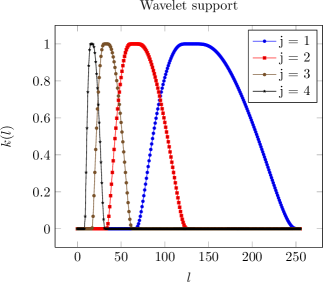
Figure 2: The figure shows the harmonic support in the frequency domain of the family of wavelets used, for $J=8$.

3.2 Pattern matching with directional wavelets

When the function $f$ from equation 4 is a wavelet, and $h$ is the signal of interest, equation 3 is the definition of the forward spherical wavelet transform, and the correlation function can be interpreted as the wavelet representation of the signal $h$.

The wavelets used in this work are defined in the harmonic domain. Their harmonic representation has the special property of allowing them to be split into a kernel and a directional part

$$b_{lm}=k(l)S_{lm},$$ (8)

where the kernel $k(l)$ is responsible for dilations and $S_{lm}$ is responsible for the directional properties of the wavelets. This split ensures that dilations do not affect directional properties, so that these two parts can be treated independently.

Table 1: First column: scale $j$. Second column: wavelet support. Third column: angular sizes in degrees for which the wavelet is sensitive. Fourth column: maximum precision on the angular variables in degrees.

$j$	Support	Angular size (∘)	Precision (∘)
$0$	$(256,128)$	$(0.7,1.4)$	$0.7$
$1$	$(256,64)$	$(0.7,2.8)$	$0.7$
$2$	$(128,32)$	$(1.4,5.6)$	$1.4$
$3$	$(64,16)$	$(2.8,11.3)$	$2.8$
$4$	$(32,8)$	$(5.6,22.5)$	$5.6$
$5$	$(16,4)$	$(11.3,45.0)$	$11.3$
$6$	$(8,2)$	$(22.5,90.0)$	$22.5$
$7$	$(4,1)$	$(45.0,180.0)$	$45.0$
$8$	$(2,1)$	$(90.0,180.0)$	$90.0$

The kernel $k(l)$ at each scale $j$ has zero values at frequencies outside the range $(2^{J-1-j},2^{J+1-j})$, where $J$ is the total number of scales. This interval is usually referred to as the wavelet support. The support is related to the frequencies to which the wavelets are sensitive. For a graphical representation see figure 2. It is interesting to notice in this figure that an adequate choice of $j$ can suppress some values of $l$, making this method powerful even when we consider the exposure of a detector, which is usually associated with low values of $l$.

In our implementation, for a given band limit $B$, the number of scales $J$ in the wavelet analysis is given by $J=\log_{2}B$. Since we have used $B=256$, then $J=8$. For a physical interpretation, however, it is simpler to think in terms of angular sizes. For that, we can convert the frequency range into angular sizes using the formula $360^{\circ}/2l$, where $l$ is the frequency we are interested in. In table 1 the angular size to which each scale is sensitive is shown.

The sensitivity of the wavelet in finding the angle $\gamma$ can be controlled by imposing a band limit on $S_{lm}$. Denoting this band limit by $N$, then $S_{lm}=0$ for all $m\geq N$. If the directional features of the signal are not relevant for the analysis, low values of $N$, such as $N=1$, can be used. The maximum value of $N$ at scale $j$ is given by $N=2^{J-j+1}$. The precision of the orientation for a given $N$ is given by $\Delta\gamma=180/N$. In this work, we have used $N=127$, shown in figure 3, which gives a precision $\Delta\gamma=1.42$ degrees. This value is a good compromise between computational resources and the required precision.

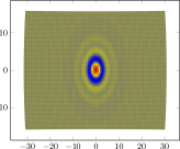
(a) $N=1$

(b) $N=127$

Figure 3: Comparison of wavelet with parameters $(J,j,N)=(8,2,1)$ and $(J,j,N)=(8,2,127)$. Both axes are in units of degrees. The wavelet shown in figure (b) is the one used in the analysis.

4 Looking for multiplets

We have developed an algorithm that uses spherical wavelets to identify and locate filaments in maps containing arrival directions of UHECRs. The algorithm is described below.

1. From a set of events, calculate the function $h(\theta,\varphi)$ that represents the signal. This involves choosing a tessellation for the sphere, and counting the total number of events contained in each pixel in the sky.

2. Calculate the Fourier expansion of $h(\theta,\varphi)$, resulting in the coefficients $a_{lm}$ (see equation 4).

3. Choose the appropriate wavelet. For the family of wavelets used, this involves choosing three parameters, the maximum scale $J$, the scale at which the analysis is performed $j$ and the azimuthal band limit, controlled by the parameter $N$. Ideally, the angular size of the wavelet will match the size of the multiplet. This choice relies on 1.

4. Calculate $C(\alpha,\beta,\gamma)$ from equation (7).

5. Select all $(\alpha,\beta,\gamma)$ such that $|C(\alpha,\beta,\gamma)|>C_{0}$, where $C_{0}$, is threshold value.

6. Select the events at each location $(\alpha,\beta,\gamma)$ (see section 4.2). This will result in $m$ groups of events.

7. Discard all groups of events for which $n<n_{0}$, where $n$ is the number of events in the group, and $n_{0}$ is a threshold value.

8. For each group of events, calculate the correlation $c$ of the graph $\delta\times 1/E$ (see equation 17).

9. Accept as a multiplet candidate all groups for which $|c|>c_{0}$, where $c_{0}$ is a threshold value. (see section 4.2)

4.1 Establishing thresholds

To carry out all steps of this algorithm one needs to establish three threshold values: the wavelet threshold $C_{0}$ used in step $5$, the minimum number of events $n_{0}$, used in step $7$, and the minimum correlation $c_{0}$, used in step $9$.

To calculate the thresholds, we have used simulated sky maps containing arrival directions of events isotropically distributed. No magnetic fields are considered in this case, so that if a multiplet is identified by our method, it certainly happened by chance. This allows us to establish the threshold values $C_{0}$, $c_{0}$, and $n_{0}$ by using the algorithm previously presented in section 4.

To estimate $c_{0}$ we use M simulations of isotropic skies, where each simulated sky follows the same injection spectrum and exposure as the data that is being analysed. $C_{i}$ is the largest wavelet coefficient obtained for each realization $i$, according to step $5$ of the algorithm.

By selecting only one value of $C$ for each realization, we have a single correlation coefficient $c_{i}$ for each of the simulated isotropic skies, calculated at step $8$ of the algorithm.

From $M$ wavelet coefficients $C_{i}$ and correlations $c_{i}$, we choose

$$C_{0}=\bar{C}+r_{C}\sigma_{C}\ \ \mbox{and}\ \ \ c_{0}=\bar{c}+r_{c}\sigma_{c},$$ (9)

where $\bar{C}$ and $\bar{c}$ denote the average values over $M$ realizations, and $\sigma_{C}$ and $\sigma_{c}$ their respective standard deviations. The numbers $r_{C}$ and $r_{c}$ are chosen according to the error the user is willing to accept. In this work we set $r_{C}=1$ and $r_{c}=1$.

The threshold value for the number of events in the multiplet, $n_{0}$, is chosen depending on the specific problem. In this analysis, for example, we have chosen $n_{0}=10$, following ref. [4].

4.2 Selecting events

To select events around the position where a wavelet has a high magnitude we need the Euler angles $\alpha$ and $\beta$, to provide a location in the sky, and the angle $\gamma$, to provide an orientation. A multiplet can, in principle, describe an arbitrary curve on the celestial sphere, depending on the intervening magnetic fields. To be general for all possible shapes we have used small segments as shown on figure 4. Each segment should be small enough so that the curve described by the events is approximately a straight line inside the segment.

A small deflection angle ($\lesssim 10^{\circ}$) can be written as $\delta=\Delta s/r$, which in spherical coordinates takes the form

$$\Delta s^{2}=r^{2}((\Delta\beta)^{2}+\sin^{2}\beta(\Delta\alpha)^{2}),$$ (10)

with $\Delta s$ being the linear distance over the surface of a sphere of radius $r$.

Now we note that the unit vectors $\hat{\alpha}$ and $\hat{\beta}$, which point in the direction where $\alpha$ and $\beta$ vary, are orthogonal and span the plane tangent to the sphere at $(\alpha,\beta)$. Using equation 10 we can write a displacement vector, tangent to that point as

$$\vec{d}=r(\Delta\beta)\hat{\beta}+r\sin\beta(\Delta\alpha)\hat{\alpha}.$$ (11)

It is convenient to write $\vec{d}$ in terms of $\hat{L}$, aligned with the wavelet, and $\hat{W}$, which is perpendicular to it. These vectors are related to $\hat{\alpha}$ and $\hat{\beta}$ by a rotation of an angle $\gamma$ in the tangent plane, as shown below:

$$\hat{\alpha} = \cos\gamma\hat{L}-\sin\gamma\hat{W}$$ (12)

$$\hat{\beta} = \sin\gamma\hat{L}-\cos\gamma\hat{W}.$$ (13)

We can now cast equation 11 as

$$\vec{d}=d_{\hat{L}}\hat{L}+d_{\hat{W}}\hat{W},$$ (14)

where

$$d_{\hat{L}} = r(\Delta\beta\cos\gamma+\sin\beta\Delta\alpha\sin\gamma)$$ (15)

$$d_{\hat{W}} = r(-\Delta\beta\sin\gamma+\sin\beta\Delta\alpha\cos\gamma).$$ (16)

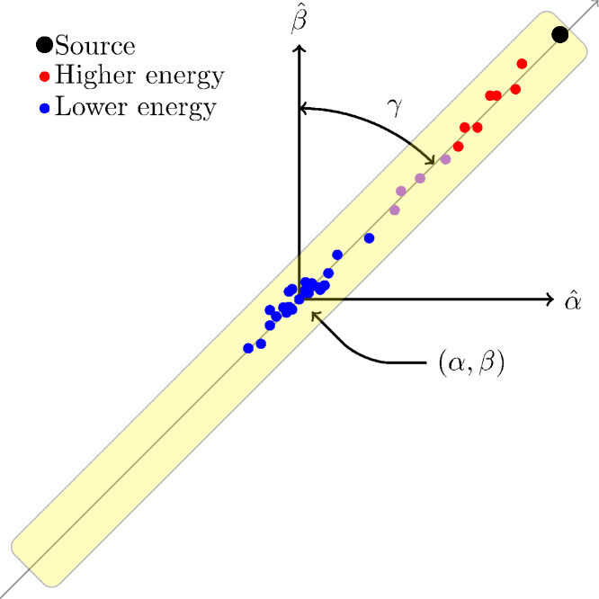
Figure 4: Illustration of a multiplet along a segment. The dots represent events from higher (red) to lower (blue) energies. The angles $(\alpha,\beta,\gamma)$ are the Euler angles associated with the multiplet.

With equations 15 and 16, we can select events in the sky at the position of maximum wavelet coefficient. The only information required are the Euler angles $\alpha$, $\beta$, and $\gamma$, since $r=1$ for the celestial sphere.

5 Analysis

To simulate both the background and the events belonging to the multiplet, we have used the software CRPropa [32]. Protons were injected following a typical $E^{-2.2}$ spectrum, for $15<E<40$ EeV. The effective detector size is a sphere of diameter 1 Mpc, and the source was assumed to be in our local universe, at a distance of 30 Mpc from the detector. If the events reach the sphere, a flag “detected” is raised. Otherwise, the events are rejected. With these settings we achieve an angular resolution of $\approx$ 1.9^∘.

For the isotropic data sets, the events were simulated in random positions of the sky.

We have divided our analysis in two parts. First we analyze an isotropic distribution of events to establish the thresholds, as explained in section 4.1. In the second part of the analysis we used a simulated multiplet composed of 10 events, embedded in the same isotropic datasets previously used. We have chosen 10 events based on [4], where 10 is the lower number of events found on a multiplet. The multiplet was simulated in the same direction each time, since by spherical symmetry the simulation is unchanged if both the source position and the magnetic field are rotated by the same angle. On the other hand, keeping the magnetic field constant and varying the source position could be a source of confusion, since the perpendicular component of the magnetic field would also vary, resulting in different multiplets each time. In the special case where event trajectories are parallel to the magnetic field, the analysis is pointless, since no multiplet is formed.

The multiplet formation was induced by an uniform magnetic field of 1 nG oriented in the $\hat{z}$ direction. Nevertheless, the results are totally independent of the method used to generate the multiplets, since it depends only on the position of the events, and on the energy- deflection correlation. The number of isotropic events range between 100 and 1000 events, in steps of 100, and a total of 1000 realizations for each of these values. The multiplet embedded in one of the isotropic skies containing 1000 isotropically distributed events can be seen in figure 5.

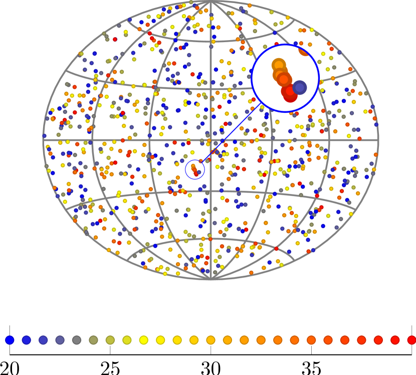
Figure 5: Simulated multiplet containing 10 events embedded in a background of 1000 events. The color scale corresponds to the energy of the events in units of EeV. The zoom shows more closely the events of the simulated multiplet.

The simulated multiplet has a correlation coefficient $c=0.99$ when no background is present. $c$ corresponds to the Pearson’s coefficient of the $\delta\times E^{-1}$ graph, given by:

$$c=\frac{\sum\limits_{i=1}^{n}\left(\frac{1}{E_{i}}-\left<\frac{1}{E}\right>\right)\sum\limits_{i=1}^{n}\left(\delta_{i}-\left<\delta\right>\right)}{\sqrt{\sum\limits_{i=1}^{n}\left(\frac{1}{E_{i}}-\left<\frac{1}{E}\right>\right)^{2}}\sqrt{\sum\limits_{i=1}^{n}\left(\delta_{i}-\left<\delta\right>\right)^{2}}}.$$ (17)

The scale at which we performed the analysis was chosen based on table 1. At scales $j=2$ and $3$ the angular size of the wavelet is close to what we would expect for a multiplet similar to the simulated one, i.e. $10^{\circ}\times 2^{\circ}$. Since at scale $j=3$ the maximum precision of the angular variable is $2.8^{\circ}$, we have used $j=2$ for the analysis. The size of the segments are $10^{\circ}\times 2^{\circ}$, to match the dimensions of the wavelet.

6 Results and Discussion

In this section we present the results of the proposed algorithm, when applied to the simulations.

Since the magnitude of the wavelet coefficients are used to select directions of interest in sky maps, i.e. Euler angles, establishing the wavelet coefficient threshold is a crucial part of the analysis. The wavelets should have enough sensitivity to distinguish the cases of interest (isotropic data sets with an embedded multiplet and without it). Figure 6 shows the average values of the magnitude of the largest wavelet coefficients found in each realization, for the two data sets. The error bars are the standard deviation of the 1000 realizations of isotropic skies. In this particular case, for a multiplet composed of 10 events, the error bars start overlapping at around 1000 events, which corresponds to a fraction of events from the multiplet with respect to the background of $\approx 10^{-2}$.

Figure 6: Magnitude of the largest wavelet coefficients in all the 1000 realizations, as a function of the number of events in the background. Blue circles correspond to the purely isotropic case, and red squares to the multiplet embedded in the isotropic background. The error bars are the standard deviation of the wavelet coefficients for all the realizations.

The correlation coefficient is the main observable to properly characterize a multiplet. In this analysis we have used $n_{0}=10$, which means that a candidate will only be considered a multiplet if it is composed by, at least, 10 events. We also have to determine the value of $c_{0}$, which is the value of the threshold correlation coefficient. It is expected that the greater the number of isotropically distributed events, which corresponds to the background, the smaller the correlation coefficient. This is corroborated by figure 7, which shows that the correlation coefficient monotonically decreases for larger number of background events, indicating a contamination of the multiplet by the background. This allows us to establish a threshold value for the correlation coefficient. For 1000 isotropic events the lowest value of $c_{0}$ considered is $c_{0}=0.4$, according to equation 9.

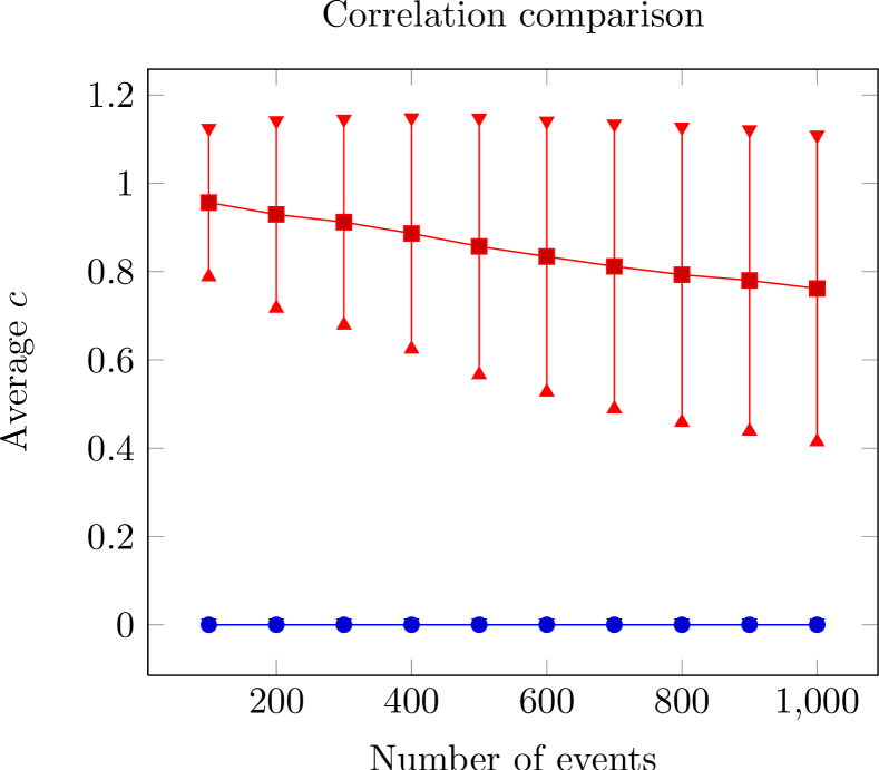
Figure 7: Correlation coefficients of the 1000 realizations, as a function of the number of events in the background. Blue circles correspond to the purely isotropic case, and red squares to the multiplet embedded in the isotropic background. The error bars are the standard deviation of the correlation coefficients for all the realizations.

It is important to address the questions related to the probability of the algorithm finding a multiplet with $c>c_{0}$ in a given data set, when no multiplets are known to be present (Type II error), and the probability of a multiplet having $c<c_{0}$ if it is known to be present in the data (Type I error). In the isotropic simulations, no multiplets with $c>0.4$ were identified for a fraction of events equal to $10^{-2}$, implying that the maximum Type II error of the method is $10^{-3}$. Figure 8 shows the Type I error introduced by our method. It is worth mentioning that for the most conservative case, which has the lowest fraction of number of events of the multiplet with respect to the number of events of the background, the Type I error introduced by using a threshold value $c_{0}=0.4$ is approximately 25%, whereas for the least conservative case it is around 2%. For a high threshold value such as $c_{0}=0.9$, this error is of the order of 30% for the most conservative case. It is important to stress that the estimated Type I and II errors depend on the confidence interval adopted, set by the parameters $r_{C}$ and $r_{c}$.

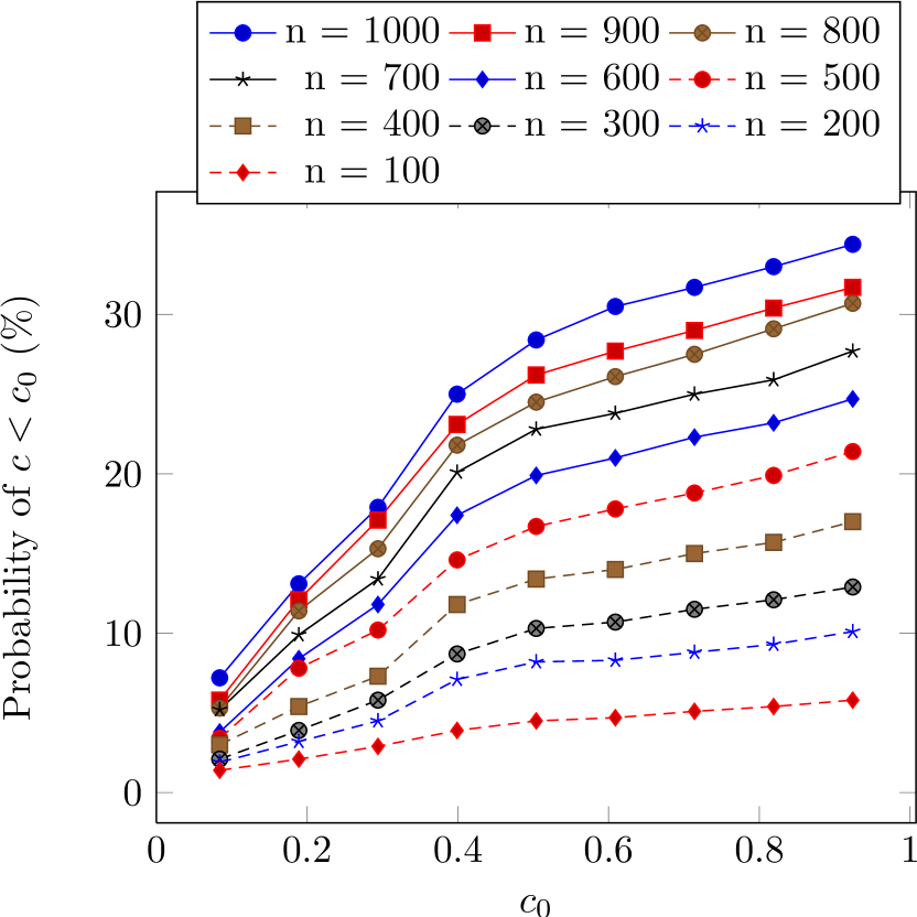
Figure 8: Probability of having $c<c_{0}$ (Type I error) when the multiplet is known to be present in the data set. Each curve corresponds to a different fraction of events of the multiplet with respect to the isotropic background.

7 Conclusion

We have developed a wavelet based analysis method to identify multiplets in maps containing arrival directions of UHECRs. We have illustrated the method by applying it to a hypothetical scenario with a uniform magnetic field of 1 nG, considering several fractions of events from the multiplet with respect to the background, down to a fraction of $10^{-2}$. All the parameters used in this study are rather arbitrary. These choices were made to illustrate the method, and not to evaluate its overall performance.

The observables used to accept or reject the multiplet candidate were the magnitude $C$ of the wavelet coefficient at the multiplet location $(\alpha,\beta,\gamma)$, the correlation $c$ of the deflection versus inverse of the energy graph and the total number of events in the multiplet $n_{0}$.

The efficiency of the method was assessed by comparing the analysis when applied to isotropically distributed events with and without an embedded multiplet. The probability of wrongly accepting a candidate multiplet with a correlation coefficient $c$ above the threshold value $c_{0}>0.4$ is below $10^{-3}$. The probability of wrongly rejecting a candidate multiplet, when it is known to be present in the data, is in the most conservative case, approximately 30%. This value goes down to 3% by decreasing the number of isotropic events in the data set. For the adopted correlation coefficient threshold, these values are, respectively, 25% and 2%.

Even though we have assumed a uniform detector exposure for the analysis previously presented, the results also hold for a non uniform exposure, since the ideal parameters for a multiplet search in the wavelet analysis suppress low frequency modes that could be related to the coverage of the cosmic ray detector. The only caveat is that, in this case, the comparison data sets should follow an isotropic distribution modulated by the exposure of the detector.

The method is focused on the search of multiplets, but it can be adapted for generic application to related problems in astrophysics, particularly the ones involving the search of filamentary structures in sky maps.

All results showed in this paper can be easily reproduced with the software SWAT (Spherical Wavelet Analysis Tool), developed by the authors of this paper. In case of interest in the code, please contact us.

References

- HiRes Collaboration [2010] HiRes Collaboration, Phys. Rev. Lett., 104 (2010) 161101. [arXiv:0910.4184]
- Pierre Auger Collaboration [2010] Pierre Auger Collaboration, Phys. Rev. Lett. (2010) 104 091101. [arXiv:1002.0699]
- Harari et al. [2002] D. Harari et al., J. High Energy Phys. 0203 (2002) 45. [astro-ph/0202362]
- Pierre Auger Collaboration [2012] Pierre Auger Collaboration, Astropart. Phys. 35 (2012) 354. [arXiv:1111.2472]
- Harari et al. [2006] D. Harari, S. Mollerach, E. Roulet, Astropart. Phys. 25 (2006) 412. [astro-ph/0602153]
- Golup et al. [2009] G. Golup et al., Astropart. Phys. 32 (2009) 269. [arXiv:0902.1742]
- Harari et al. [1999] D. Harari, S. Mollerach, E. Roulet, J. High Energy Phys. 8 (1999) 22. [astro-ph/9906309]
- Sun et al. [2008] X. H. Sun et al., Astron. Astrophys. 477 (2008) 573. [arXiv:0711.1572]
- Pshirkov et al. [2011] M. S. Pshirkov et al., Astrophys. J. 738 2 (2011) 192. [arXiv:1103.0814]
- Jansson & Farrar [2012] R. Jansson, G. Farrar, Astrophys. J., 757 (2012) 14. [arXiv:1204.3662]
- Sigl et al. [2003] G. Sigl, F. Miniati, T. Ensslin, Phys. Rev. D 68 (2003) 043002. [astro-ph/0302388]
- Dolag et al. [2005] K. Dolag et al., JCAP 1 (2005) 9. [astro-ph/0410419]
- Armengaud et al. [2005] E. Armengaud, G. Sigl, F. Miniati, Phys. Rev. D 72 (2005) 043009. [astro-ph/0412525]
- Das et al. [2008] S. Das et al., Astrophys. J. 682 7 (2008) 29. [arXiv:0801.0371]
- Cayón et al. [1999] L. Cayón et al., in de Oliveira-Costa A., Tegmark M., eds, Microwave Foregrounds. ASP Conference Series 181 (1999) 349.
- Sanz et al. [1999] J. L. Sanz et al., Mon. Not. R. Astr. Soc. 309 (1999) 672. [astro-ph/9906367]
- González-Nuevo et al. [2006] J. González-Nuevo et al., Mon. Not. R. Astr. Soc. 369 (2006) 1603. [astro-ph/0604376]
- Faÿ et al. [2011] G. Faÿ et al., (2011). [arXiv:1107.5658]
- Alves Batista et al. [2010] R. Alves Batista et al. Physicæ Proceedings 1 (2010) 1-6. [arXiv:1201.2183]
- Alves Batista et al. [2011] R. Alves Batista, E. Kemp, B. Daniel, Int. J. Mod. Phys. E 20 (2011) 61-66. [arXiv:1201.2799]
- Ivanov et al. [2003a] A. A. Ivanov, A. D. Krasilnikov, M. I. Pravdin, JETP Lett. 78 (2003) 695.
- Ivanov et al. [2003b] A. A. Ivanov, A. D. Krasilnikov, M. I. Pravdin, International Cosmic Ray Conference 1 (2003) 341.
- Martínez-González et al. [2002] Martínez-González E. et al., Mon. Not. R. Astr. Soc. 336 (2002) 22. [astro-ph/0111284]
- McEwen et al. [2006a] J. D. McEwen et al., Mon. Not. R. Astr. Soc. 369 (2006) 1858. [astro-ph/0510349]
- McEwen et al. [2006b] J. D. McEwen et al., J. Fourier Anal. Appl. 13 (2006) 495. [arXiv:0704.3158]
- McEwen et al. [2008a] J. D. McEwen et al., Mon. Not. R. Astr. Soc. 388 (2008) 659. [arXiv:0803.2157]
- McEwen et al. [2007] J. D. McEwen et al., Society of Photo-Optical Instrumentation Engineers (SPIE) Conference Series 6701 (2007) 670115. [arXiv:0708:3874]
- McEwen et al. [2008b] J. D. McEwen et al., Mon. Not. R. Astr. Soc. 384 (2008) 1289. [arXiv:0704.0626]
- Kovacs & Wriggers [2002] J. A. Kovacs, W. Wriggers, Acta Crystallogr. D. 58 (2002) 1282.
- Kostelec & Rockmore [2008] P. Kostelec, D. Rockmore, J. Fourier Anal. Appl. 14 (2008) 145.
- Wiaux et al. [2008] Y. Wiaux et al., Mon. Not. R. Astr. Soc. 388 (2008) 770. [arXiv:0712.3519]
- Kampert et al. [2007] K.-H. Kampert et al., Astropart. Phys. 42 (2013) 41. [arXiv:1206.3132]