Probe and Adapt: Rate Adaptation for HTTP Video Streaming At Scale

Abstract

Today, the technology for video streaming over the Internet is converging towards a paradigm named HTTP-based adaptive streaming (HAS), which brings two new features. First, by using HTTP/TCP, it leverages network-friendly TCP to achieve both firewall/NAT traversal and bandwidth sharing. Second, by pre-encoding and storing the video in a number of discrete rate levels, it introduces video bitrate adaptivity in a scalable way so that the video encoding is excluded from the closed-loop adaptation. A conventional wisdom is that the TCP throughput observed by an HAS client indicates the available network bandwidth, and thus can be used as a reliable reference for video bitrate selection.

We argue that this is no longer true when HAS becomes a substantial fraction of the total traffic. We show that when multiple HAS clients compete at a network bottleneck, the presence of competing clients and the discrete nature of the video bitrates together result in difficulty for a client to correctly perceive its fair-share bandwidth. Through analysis and test bed experiments, we demonstrate that this fundamental limitation leads to, for example, video bitrate oscillation that negatively impacts the video viewing experience. We therefore argue that it is necessary to design at the application layer using a “probe-and-adapt” principle for HAS video bitrate adaptation, which is akin to, but also independent of the transport-layer TCP congestion control. We present PANDA – a client-side rate adaptation algorithm for HAS – as practical embodiment of this principle. Our test bed results show that compared to conventional algorithms, PANDA is able to reduce the instability of video bitrate selection by over 75% without increasing the risk of buffer underrun.

I Introduction

Over the past few years, we have witnessed a major technology convergence for Internet video streaming towards a new paradigm named HTTP-based adaptive streaming (HAS). Since its inception in 2007 by Move Networks [1], HAS has been quickly adopted by major vendors and service providers. Today, HAS is employed for over-the-top video delivery by many major media content providers. A recent report by Cisco [7] predicts that video will constitute more than 90% of the total Internet traffic by 2014. Therefore, HAS may become a predominant form of Internet traffic in just a few years.

In contrast to conventional RTP/UDP-based video streaming, HAS uses HTTP/TCP – the protocol stack traditionally used for Web traffic. In HAS, a video stream is chopped into short segments of a few seconds each. Each segment is pre-encoded and stored at a server in a number of versions, each with a distinct video bitrate, resolution and/or quality. After obtaining a manifest file with necessary information, a client downloads the segments sequentially using plain HTTP GETs, estimates the network conditions, and selects the video bitrate of the next segment on-the-fly. A conventional wisdom is that since the bandwidth sharing of HAS is dictated by TCP, the problem of video bitrate selection can be resolved straightforwardly. A simple rule of thumb is to approximately match the video bitrate to the observed TCP throughput.

Fetched Bitrate Aggregated over 36 Streams

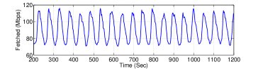
Fetched Bitrate of Individual Streams (Zoom In)

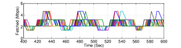
Figure 1: Oscillation of video bitrate when 36 Microsoft Smooth clients compete at a 100-Mbps link. For more detailed experimental setup, refer to $\S$VI-B.

I-A Emerging Issues

A major trend in HAS use cases is its large-scale deployment in managed networks by service providers, which typically leads to aggregating multiple HAS streams in the aggregation/core network. For example, an important scenario is that within a single household or a neighborhood, several HAS flows belonging to one DOCSIS bonding group compete for bandwidth. In the unmanaged wide-area Internet, as HAS is growing to become a substantial fraction of the total traffic, it will also become more and more common to have multiple HAS streams compete for available bandwidth at any network bottlenecks.

While a simple rate adaptation algorithm might work fairly well for the case where a single HAS stream operates alone or shares bandwidth with non-HAS traffic, recent studies [13, 3] have reported undesirable behaviors when multiple HAS streams compete for bandwidth at a bottleneck link. For example, while studies have suggested that significant video quality variation over time is undesirable for a viewer’s quality of experience [18], in [13] the authors reported unstable video bitrate selection and unfair bandwidth sharing among three Microsoft Smooth clients sharing a 3-Mbps link. In our own test bed experiments (see Figure 1), we observed significant and regular video bitrate oscillation when multiple Microsoft Smooth clients share a bottleneck link. We also found that oscillation behavior persists under a wide range of parameter settings, including the number of players, link bandwidth, start time of clients, heterogeneous RTTs, random early detection (RED) queueing parameters, the use of weight fair queueing (WFQ), the presence of moderate web-like cross traffic, etc.

Our study shows that these HAS rate oscillation and instability behaviors are not incidental – they are simply symptoms of a much more fundamental limitation of the conventional HAS rate adaptation algorithms, in which the TCP downloading throughput observed by a client is directly equated to its fair share of the network bandwidth. This fundamental problem would also impact a HAS client’s ability to avoid buffer underrun when the bandwidth suddenly drops. In brief, the problem derives from the discrete nature of HAS video bitrates. This makes it impossible to always match the video bitrate to the network bandwidth, resulting in undersubscription of the network bandwidth. Undersubscription is typically coupled with clients’ on-off downloading patterns. The off-intervals then become a source of ambiguity for a client to correctly perceive its fair share of the network bandwidth, thus preventing the client from making accurate rate adaptation decisions.

I-B Overview of Solution

To overcome this fundamental limitation, we envision a solution based on a “probe-and-adapt” principle. In this approach, the TCP downloading throughput is taken as an input only when it is an accurate indicator of the fair-share bandwidth. This usually happens when the network is oversubscribed (or congested) and the off-intervals are absent. In the presence of off-intervals, the algorithm constantly probes the network bandwidth by incrementing its sending rate, and prepares to back off once it experiences congestion. This new mechanism shares the same spirit with TCP’s congestion control, but it operates independently at the application layer and at a per-segment rather than a per-RTT time scale. We present PANDA (Probe AND Adapt) – a client-side rate adaptation algorithm – as a specific implementation of this principle.

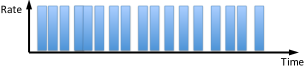
(a) PANDA

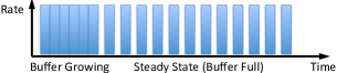
(b) Conventional Bimodal

Figure 2: Illustration of PANDA’s fine-granular request intervals vs. a conventional algorithm’s bimodal request intervals.

Probing constitutes fine-tuning the requested network data rate, with continuous variation over a range. By nature, the available video bitrates in HAS can only be discrete. A main challenge in our design is to create a continuous decision space out of the discrete video bitrate. To this end, we propose to fine-tune the intervals between consecutive segment download requests such that the average data rate sent over the network is a continuous variable (see Figure 2 for an illustrative comparison with the conventional scheme). Consequently, instead of directly tuning the video bitrate, we probe the bandwidth based on the average data rate, which in turn determines the selected video bitrate and the fine-granularity inter-request time.

There are various benefits associated with the probe-and-adapt approach. First, it avoids the pitfall of inaccurate bandwidth estimation. Having a robust bandwidth measurement to begin with gives the subsequent operations improved discriminative power (for example, strong smoothing of the bandwidth measurement is no longer required, leading to better responsiveness). Second, with constant probing via incrementing the rate, the network bandwidth can be more efficiently utilized. Third, it ensures that the bandwidth sharing converges towards fair share (i.e., the same or adjacent video bitrate) among competing clients. Lastly, an innate feature of the probe-and-adapt approach is asymmetry of rate shifting – PANDA is equipped with conservative rate level upshift but more responsive downshift. Responsive downshift facilitates fast recovery from sudden bandwidth drops, and thus can effectively mitigate the danger of playout stalls caused by buffer underrun.

Notation	Explanation
$w$	Probing additive increase bitrate
$\kappa$	Probing convergence rate
$\alpha$	Smoothing convergence rate
$\beta$	Client buffer convergence rate
$\Delta$	Quantization margin
$\epsilon$	Multiplicative safety margin
$\tau$	Video segment duration (in video time)
$B$	Client buffer duration (in video time)
$B_{\min}$; $B_{\max}$	Minimum/maximum client buffer duration
$T$	Actual inter-request time
$\hat{T}$	Target inter-request time
$\tilde{T}$	Segment download duration
$x$	Actual average data rate
$\hat{x}$	Target average data rate (or bandwidth share)
$\hat{y}$	Smoothed version of $\hat{x}$
$\tilde{x}$	TCP throughput measured, $\tilde{x}:=\frac{r\cdot\tau}{\tilde{T}}$
$\mathcal{R}$	Set of video bitrates $\mathcal{R}:=\{R_{1},...,R_{L}\}$
$r$	Video bitrate available from $\mathcal{R}$
$S(\cdot)$	Rate smoothing function
$Q(\cdot)$	Video bitrate quantization function

TABLE I: Notations used in this paper

I-C Paper Organization

In the rest of the paper, after formalizing the problem ($\S$II), we first introduce a method to characterize the conventional rate adaptation algorithms ($\S$III), based on which we analyze the root cause of its problems ($\S$IV). We then introduce our probe-and-adapt approach ($\S$V) to directly address the root cause, and present the PANDA rate adaptation algorithm as a concrete implementation of this idea. We provide comprehensive performance evaluations ($\S$VI). We conclude the paper with final remarks and discussion of future work ($\S$VIII).

II Problem Model

In this section, we formalize the problem by first describing a representative HAS server-client interaction process. We then outline a four-step model for an HAS rate adaptation algorithm. This will allow us to compare the proposed PANDA algorithm with its conventional counterpart. Table I lists the main notations used in this paper.

II-A Process of HAS Server-Client Interaction

Consider that a video stream is chopped into segments of $\tau$ seconds each. Each segment has been pre-encoded at $L$ video bitrates, all stored at a server. Denote by $\mathcal{R}:=\{R_{1},...,R_{L}\}$ the set of available video bitrates, with $0<R_{\ell}<R_{m}$ for $\ell<m$.

For each client, the streaming process is divided into sequential segment downloading steps $n=1,2,...$. The process we consider here generalizes the process used by conventional HAS clients by further incorporating variable durations between consecutive segment requests. Refer to Figure 3. At the beginning of each download step $n$, a rate adaptation algorithm:

• Selects the video bitrate of the next segment to be downloaded, $r[n]\in\mathcal{R}$;

• Specifies how much time to give for the current download, until the next download request (i.e., the inter-request time), $\hat{T}[n]$.

The client then initiates an HTTP GET request to the server for the segment of sequence number $n$ and video bitrate $r[n]$, and the downloading starts immediately. Let $\tilde{T}[n]$ be the download duration – the time required to complete the download. Assuming that no pipelining of downloading is involved, the next download step starts after time

$$T[n]=\max(\hat{T}[n],\tilde{T}[n]),$$ (1)

where $T[n]$ is the actual inter-request time. That is, if the download duration $\tilde{T}[n]$ is shorter than the target delay $\hat{T}[n]$, the client waits time $\hat{T}[n]-\tilde{T}[n]$ (i.e., the off-interval) before starting the next downloading step (Scenario A); otherwise, the client starts the next download step immediately after the current download is completed (Scenario B).

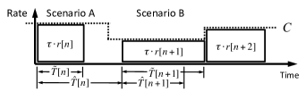
Figure 3: The HAS segment downloading process.

Typically, a rate adaptation algorithm also measures its TCP throughput $\tilde{x}$ during the segment downloading, via:

$$\tilde{x}[n]:=\frac{r[n]\cdot\tau}{\tilde{T}[n]}.$$

The downloaded segments are stored in the client buffer. After playout starts, the buffer is consumed by the video player at a natural rate of one video second per real second on average. Let $B[n]$ be the buffer duration (measured in video time) at the end of step $n$. Then the buffer dynamics can be characterized by:

$$B[n]=\max\left(0,B[n-1]+\tau-T[n]\right).$$ (2)

II-B Four-Step Model

We present a four-step model for an HAS rate adaptation algorithm, generic enough to encompass both the conventional algorithms (e.g., [15, 19, 20, 17, 16]) and the proposed PANDA algorithm. In this model, a rate adaptation algorithm proceeds in the following four steps.

• Estimating. The algorithm starts by estimating the network bandwidth $\hat{x}[n]$ that can legitimately be used.

• Smoothing. $\hat{x}[n]$ is then noise-filtered to yield the smoothed version $\hat{y}[n]$, with the aim of removing outliers.

• Quantizing. The continuous $\hat{y}[n]$ is then mapped to the discrete video bitrate $r[n]\in\mathcal{R}$, possibly with the help of side information such as client buffer size, etc.

• Scheduling. The algorithm selects the target interval until the next download request, $\hat{T}[n]$.

III Conventional Approach

Using the four-step model above, in this section we introduce a scheme to characterize a conventional rate adaptation algorithm, which will serve as a benchmark.

To the best of our knowledge, almost all of today’s commercial HAS players implement the measuring and scheduling parts of the rate adaptation algorithm in a similar way, though they may differ in their implementation of the smoothing and quantizing parts of the algorithm. Our claim is based on a number of experimental studies of commercial HAS players [2, 10, 13]. The scheme described in Algorithm 1 characterizes their essential ideas.

At the beginning of each downloading step $n$:

1. Estimate the bandwidth share $\hat{x}[n]$ by equating it to the measured TCP throughput:

   $$\hat{x}[n]=\tilde{x}[n-1].$$ (3)

2. Smooth out $\hat{x}[n]$ to produce filtered version $\hat{y}[n]$ by

   $$\hat{y}[n]=S(\{\hat{x}[m]:m\leq n\}).$$ (4)

3. Quantize $\hat{y}[n]$ to the discrete video bitrate $r[n]\in\mathcal{R}$ by

   $$r[n]=Q\left(\hat{y}[n];...\right).$$ (5)

4. Schedule the next download request depending on the buffer fullness:

   $$\hat{T}[n]=\begin{cases}0,&B[n-1]<B_{\max},\\ \tau,&\mathrm{otherwise.}\end{cases}$$ (6)

Algorithm 1 Conventional

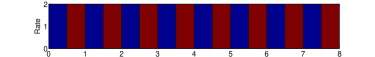
(a) Perfectly Subscribed, Round-Robin

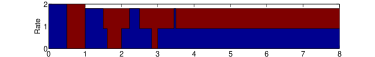
(d) Oversubscribed

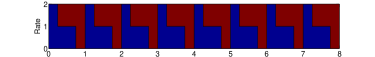
(b) Perfectly Subscribed, Partially Overlapped

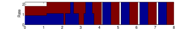
(e) Undersubscribed

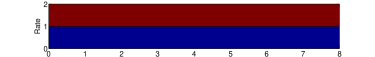
(c) Perfectly Subscribed, Fully Overlapped

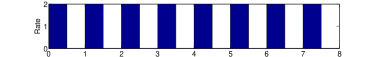
(f) Single-Client

Figure 4: Illustration of various bandwidth sharing scenarios. In (a), (b) and (c), the link is perfectly subscribed. In (d), the bandwidth sharing starts with round-robin mode but then link becomes oversubscribed. In (e), the bandwidth sharing starts with fully overlapped mode when the link is oversubscribed. Starting from the second round, the link becomes undersubscribed. In (f), a single client is downloading, and the downloading on-off pattern exactly matches that of the blue segments in (a).

First, the algorithm equates the currently available bandwidth share $\hat{x}[n]$ to the past TCP throughput $\tilde{x}[n-1]$ observed during the on-interval $\tilde{T}[n-1]$. As the bandwidth is inferred reactively based on the previous downloads, we refer to this as reactive bandwidth estimation.

The algorithm then obtains a filtered version $\hat{y}[n]$ using a smoothing function $S(\cdot)$ that takes as input the measurement history $\{\hat{x}[m]:m\leq n\}$, as described in (4). Various filtering methods are possible, such as sliding-window moving average, exponential weighted moving average (EWMA) or harmonic mean [13].

The next step maps the continuous $\hat{y}[n]$ to a discrete video bitrate $r[n]\in\mathcal{R}$ using a quantization function $Q(\cdot)$. In general, $Q(\cdot)$ can also incorporate side information, including the past fetched bitrates $\{r[m]:m<n\}$ and the buffer history $\{B[m]:m<n\}$.

Lastly, the algorithm determines the target inter-request time $\hat{T}[n]$. In (6), $\hat{T}[n]$ is a mechanical function of the buffer duration $B[n-1]$. If $B[n-1]$ is less than a pre-defined maximum buffer $B_{\max}$, $\hat{T}[n]$ is set to $0$, and by (1), the next segment downloading starts right after the current download is finished; otherwise, the inter-request time is set to the video segment duration $\tau$, to stop the buffer from further growing. This creates two distinct modes of segment downloading – the buffer growing mode and the steady-state mode, as shown in Figure 2(b). We refer to this as the bimodal download scheduling.

IV Analysis of the Conventional Approach

In this section, we take a deep dive into the conventional rate adaptation algorithms and study their limitations.

IV-A Bandwidth Cliff Effect

As we have seen in the previous section, conventional rate adaptation algorithms use reactive bandwidth estimation (3) that equates the estimated bandwidth share to the TCP throughput observed during the on-intervals. In the presence of competing HAS clients, however, the TCP throughput does not always faithfully represent the fair-share bandwidth. In this section, we present an intuitive analysis of this phenomenon, by extending the one first presented in [3]. A rigorous analysis of this phenomenon is presented in Appendix A.

First, we illustrate with simple examples. Figure 4 (a) - (e) show the various scenarios of how a link can be shared by two HAS clients in steady-state mode. We consider three different scenarios: perfect link subscription, link oversubscription and link undersubscription. We assume ideal TCP behavior, i.e., perfectly equal sharing of the available bandwidth when the transfers overlap.

Perfect Subscription: In perfect link subscription, the total amount of traffic requested by the two clients perfectly fills the link. (a), (b) and (c) illustrate three different modes of bandwidth sharing, depending on the starting time of downloads relative to each other. Essentially, under perfect subscription, there are unlimited number of bandwidth sharing modes.

Oversubscription: In (d), the two clients start with round-robin mode and perfect subscription. Starting from the second round of downloading, the bandwidth is reduced and the link becomes oversubscribed, i.e., each client requests segments larger than its current fair-share portion of the bandwidth. This will result in unfinished downloads at the end of each downloading round. Then, the unfinished segment will start overlapping with segments of the next round. This repeats and the downloading will become more and more overlapped, until all the clients enter the fully overlapped mode.

Undersubscription: In (e), initially the bandwidth sharing is in fully overlapped mode, and the link is oversubscribed. Starting from the second round, the bandwidth increases and the link becomes undersubscribed. Then the clients start filling up each other’s off-intervals, until a transmission gap emerges. The bandwidth sharing will eventually converge to a mode which is determined by the download start times.

In any case, the measured TCP throughput faithfully represents the fair-share bandwidth only when the bandwidth sharing is in the fully overlapped mode; in all other cases the TCP throughput overestimates the fair-share bandwidth. Thus, most of the time, the bandwidth estimate is accurate when the link is oversubscribed. Bandwidth overestimation occurs when the link is undersubscribed or perfectly subscribed. In general, when the number of competing clients is $n$, the bandwidth overestimation ranges from one to $n$ times the fair-share bandwidth.

Although the preceding simple examples assume idealized TCP behavior which abstracts away the complexity of TCP congestion control dynamics, it is easy to verify that similar behavior occurs with real TCP connections. To see this, we conducted a simple test bed experiment as follows. We implemented a “thin client” to mimic an HAS client in the steady-state mode. Each thin client repeatedly downloads a segment every 2 seconds. We run 100 instances of the thin client sharing a bottleneck link of 100 Mbps, each with a starting time randomly selected from a uniform distribution between 0 and 2 seconds. Figure 5 plots the measured average TCP throughput as a function of the link subscription rate. We observe that when the link subscription is below 100%, the measured throughput is about 3x the fair-share bandwidth of ~1 Mbps. When the link subscription is above 100%, the measured throughput successfully predicts the fair-share bandwidth quite accurately. We refer to this sudden transition from overestimation to fairly accurate estimation of the bandwidth share at 100% subscription as the bandwidth cliff effect.

We summarize our findings as follows:

• Link oversubscription converges to fully overlapped bandwidth sharing and accurate bandwidth estimation.

• Link undersubscription converges to a bandwidth sharing pattern determined by the download start times and bandwidth overestimation.

• In perfect link subscription, there exist unlimited bandwidth sharing modes, leading to bandwidth overestimation.

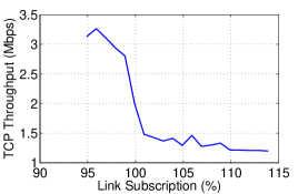
Figure 5: Bandwidth cliff effect: measured TCP throughput vs. link subscription rate for 100 thin clients sharing a 100-Mbps link. Each thin client repeatedly downloads a segment every $\tau=2$ seconds.

IV-B Video Bitrate Oscillation

With an understanding of the bandwidth cliff effect, we are now in a good position to explain the bitrate oscillation observed in Figure 1.

Figure 6 illustrates this process. When the client buffer reaches the maximum level $B_{\max}$, by (6), off-intervals start to emerge. The link becomes undersubscribed, leading to bandwidth overestimation (a). This triggers the upshift of requested video bitrate (b). As the available bandwidth cannot keep up with the video bitrate, the buffer falls below $B_{\max}$. By (6), the client falls back to the buffer growing mode and the off-intervals disappear, in which case the link again becomes oversubscribed and the measured throughput starts to converge to the fair-share bandwidth (c). Lastly, due to the quantization effect, the requested video bitrate falls below the fair-share bandwidth (d), and the client buffer starts growing again, completing one oscillation cycle.

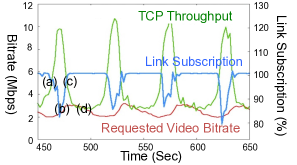
Figure 6: Illustration of vicious cycle of video bitrate oscillation. This plot is obtained with 36 Smooth clients sharing a 100-Mbps link. For experimental setup, refer to $\S$VI-B.

IV-C Fundamental Limitation

The bandwidth overestimation phenomenon reveals a more general and fundamental limitation of the class of conventional reactive bandwidth estimation approaches discussed so far. As video bitrates are chosen solely based on measured TCP throughput from past segment downloads during the on-intervals, such decisions completely ignore the network conditions during the off-intervals. This leads to an ambiguity of client knowledge of available network bandwidth during the off-intervals, which, in turn, hampers the adaptation process.

To illustrate this point, consider two alternative scenarios as depicted in Figures 4 (f) and (a). In (f), the client downloading the blue (darker-shaded) video segments occupies the link alone; in (a), it shares the same link with a competing client downloading the green (lighter-shaded) video segments. Note that the on/off-intervals for all the blue (darker-shaded) video segments follow exactly the same pattern in both scenarios. Consequently, the client observes exactly the same TCP throughput measurement over time. If the client would obtain a complete picture of the network, it would know to upshift its video bitrate in (f) but retain its current bitrate in (a). In practice, however, an individual client cannot distinguish between these two scenarios, hence, is bound to the same behavior in both.

Note that as long as the off-intervals persist, such ambiguity in client knowledge is inherent to the bandwidth measurement step in a network with competing streams. It cannot be resolved or remedied by improved filtering, quantization, or scheduling steps performed later in the client adaptation algorithm. Moreover, the bandwidth cliff effect, as discussed in Section IV-A, suggests that the bandwidth overestimation problem does not improve with more clients, and that it can introduce large errors even with slight link undersubscription.

Instead, the client needs to take a more proactive approach in adapting the video bitrate — whenever it is known that the client knowledge is impaired, it must avoid using such knowledge in bandwidth estimation. A way to distinguish the case when the knowledge is impaired from when it is not, is to probe the network subscription by small increment of its data sending rate. We describe one algorithm that follows such an alternative approach in the next section.

V Probe-and-Adapt Approach

In this section, we introduce our proposed probe-and-adapt approach to directly address the root cause of the conventional algorithms’ problems. We begin the discussion by laying out the design goals that a rate adaptation algorithm aims to achieve. We then describe the PANDA algorithm as an embodiment of the probe-and-adapt approach, and provide its functional verification using experimental traces.

V-A Design Goals

Designing an HAS rate adaptation algorithm involves tradeoffs among a number of competing goals. It is not legitimate to optimize one goal (e.g., stability) without considering its tradeoff factors. From an end-user’s perspective, an HAS rate adaptation algorithm should be designed to meet these criteria:

• Avoiding buffer underrun. Once the playout starts, buffer underrun (i.e., complete depletion of buffer) leads to a playout stall. Empirical study [8] has shown that buffer underrun may have the most severe impact on a user’s viewing experience. To avoid it, some minimal buffer level must be maintained at all times, and the adaptation algorithm must be highly responsive to network bandwidth drops.

• High quality smoothness. In the simplest setting without considering visual perceptual models, high video quality smoothness translates into avoiding both frequent and significant video bitrate shifts among available video bitrate levels [13, 18].

• High average quality. High average video quality dictates that a client should fetch high-bitrate segments as much as possible. Given a fixed network bandwidth, this translates into high network utilization.

• Fairness. In the simplest setting, fairness translates into equal network bandwidth sharing among competing clients.

Note that this list above is non-exhaustive. Other criteria, such as low playout startup latency, are also important factors impacting user’s viewing experience.

V-B PANDA Algorithm

In this section, we discuss the PANDA algorithm. Compared to the reactive bandwidth estimation used by a conventional rate adaptation algorithm, PANDA uses a more proactive probing mechanism. By probing, PANDA determines a target average data rate $\hat{x}$. This average data rate is subsequently used to determine the video bitrate $r$ to be fetched, and the interval $\hat{T}$ until the next segment download request.

The PANDA algorithm is described in Algorithm 2, and a block diagram interpretation of the algorithm is shown in Figure 7. Compared to the conventional algorithm in Algorithm 1, we only make modifications in the estimating and scheduling steps – we replace (3) with (7) for estimating the bandwidth share, and (6) with (10) for scheduling the next download request. We now focus on elaborating each of these two modifications.

At the beginning of each downloading step $n$:

1. Estimate the bandwidth share $\hat{x}[n]$ by

   $$\frac{\hat{x}[n]-\hat{x}[n-1]}{T[n-1]}=\kappa\cdot(w-\max(0,\hat{x}[n-1]-\tilde{x}[n-1])),$$ (7)

2. Smooth out $\hat{x}[n]$ to produce filtered version $\hat{y}[n]$ by

   $$\hat{y}[n]=S(\{\hat{x}[m]:m\leq n\}).$$ (8)

3. Quantize $\hat{y}[n]$ to the discrete video bitrate $r[n]\in\mathcal{R}$ by

   $$r[n]=Q\left(\hat{y}[n];...\right).$$ (9)

4. Schedule the next download request via

   $$\hat{T}[n]=\frac{r[n]\cdot\tau}{\hat{y}[n]}+\beta\cdot\left(B[n-1]-B_{\min}\right)$$ (10)

Algorithm 2 PANDA

Figure 7: Block diagram for PANDA (Algorithm 2). Module D represents delay of one adaptation step.

In the estimating step, (7) is designed to directly address the root cause that leads to the video bitrate oscillation phenomenon. Based on the insights obtained from $\S$IV-A, when the link becomes undersubscribed, the direct TCP throughput estimate $\tilde{x}$ becomes inaccurate in predicting the fair-share bandwidth, and thus should be avoided. Instead, the client continuously increments the target average data rate $\hat{x}$ by $\kappa\cdot w$ per unit time as a probe of the available capacity. Here $\kappa$ is the probing convergence rate and $w$ is the additive increase rate. The algorithm keeps on monitoring the TCP throughput $\tilde{x}$, and compares it against the target average data rate $\hat{x}$. If $\tilde{x}>\hat{x}$, $\tilde{x}$ would not be informative, since in this case the link may still be undersubscribed and $\tilde{x}$ may overestimate the fair-share bandwidth. Thus, its impact is suppressed by the $\max(0,\cdot)$ function. But if $\tilde{x}<\hat{x}$, then TCP throughput cannot keep up with the target average data rate indicates that congestion has occurred. This is when the target data rate $\hat{x}$ should back off. The reduction imposed on $\hat{x}$ is made proportional to $\hat{x}-\tilde{x}$. Intuitively, the lower the measured TCP throughput $\tilde{x}$, the more reduction that needs to be imposed on $\hat{x}$. This design makes our rate adaptation algorithm very agile to bandwidth changes.

PANDA’s probing mechanism shares similarities with TCP’s congestion control [11], and has an additive-increase-multiplicative-decrease (AIMD) interpretation: $\kappa\cdot w$ is the additive increase term, and $-\kappa\cdot\max(0,\hat{x}[n-1]-\tilde{x}[n-1])$ can be interpreted as the multiplicative decrease term. The main difference is that in TCP, congestion is indicated by packet losses (TCP Reno) or increased round-trip time (delay-based TCP), whereas in (7), congestion is indicated by the reduction of measured TCP throughput. This AIMD property ensures that PANDA is able to efficiently utilize the network bandwidth, and in the presence of multiple clients, the bandwidth for each client eventually converges to fair-share status.

In the scheduling step, (10) aims to determine the target inter-request time $\hat{T}[n]$. By right, $\hat{T}[n]$ should be selected such that the smoothed target average data rate $\hat{y}[n]$ is equal to $\frac{r[n]\cdot\tau}{\hat{T}[n]}$. But additionally, the selection of $\hat{T}[n]$ should also drive the buffer $B[n]$ towards a minimum reference level $B_{\min}>0$, so the second term is added to the right hand side of (10), where $\beta>0$ controls the convergence rate.

One distinctive feature of the PANDA algorithm is its hybrid closed-loop/open-loop design. Refer to Figure 7. In this system, (7) forms a closed loop by itself that determines the target average data rate $\hat{x}$. (10) forms a closed loop by itself that determines the target inter-request time $\hat{T}$. Overall, the estimating, smoothing, quantizing and scheduling steps together form an open loop. The main motivation behind this design is to reduce the bitrate shifts associated with quantization. Since quantization is excluded from the closed loop of $\hat{x}$, it allows $\hat{x}$ to settle in a steady state. Since $r[n]$ is a deterministic function of $\hat{x}[n]$, it can also settle in a steady state.

In Appendix B, we present an equilibrium and stability analysis of PANDA. We summarize the main results as follows. Our equilibrium analysis shows that at steady state, the system variables settle at

$$\hat{x}_{o} = \tilde{x}_{o}+w$$

$$= \hat{y}_{o}$$

$$r_{o} = Q(\hat{x}_{o};...)$$

$$B_{o} = \left(1-\frac{r_{o}}{\hat{y}_{o}}\right)\cdot\frac{\tau}{\beta}+B_{\min},$$ (12)

where the subscript $o$ denotes value of variables at equilibrium. Our stability analysis shows that for the system to converge towards the steady state, it is necessary to have:

$$\kappa < \frac{2}{\tau}$$ (13)

$$w \leq \Delta,$$ (14)

where $\Delta$ is a parameter associated with the quantizer $Q(\cdot)$, referred to as the quantization margin, i.e., the selected discrete rate $r$ must satisfy

$$r[n]\leq\hat{y}[n]-\Delta.$$ (15)

V-C Functional Verification

We verify the behavior of PANDA using experimental traces. For detailed experiment setup (including the selection of function $S(\cdot)$ and $Q(\cdot)$), refer to $\S$VI-B.

First, we evaluate how a single PANDA client adjusts its video bitrate as the the available bandwidth varies over time. In Figure 8, we plot the TCP throughput $\tilde{x}$, the target average data rate $\hat{x}$, the fetched video bitrate $r$ and the client buffer $B$ for a duration of 500 seconds, where the bandwidth drops from 5 to 2 Mbps at 200 seconds, and rises back to 5 Mbps at 300 seconds. Initially, the target average data rate $\hat{x}$ ramps up gradually over time; the fetched video bitrate $r$ also ramps up correspondingly. After the initial ramp-up stage, $\hat{x}$ settles in a steady state. It can be observed that at steady state, the difference between $\hat{x}$ and $\tilde{x}$ is about 0.3 Mbps, equal to $w$, which is consistent with (V-B). Similarly, the buffer $B$ also settles in a steady state, and after plugging in all the parameters, one can verify that the steady state of buffer (12) also holds. At 200 seconds, when the bandwidth suddenly drops, the fetched video bitrate quickly drops to the desirable level. With this quick response, the buffer hardly drops. This property makes PANDA favorable for live streaming applications. When the bandwidth rises back to 5 Mbps at 300 seconds, the fetched video bitrate gradually ramps up to the original level.

Note that, in practical implementation, we can further add a startup logic to improve PANDA’s ramp-up speed at the stream startup stage, akin to the slow-start mode of TCP. The idea is simple: since it is necessary to add off-intervals only when the buffer duration $B[n]$ exceeds the minimum reference level $B_{\min}$, we can use the conventional algorithm at startup or after playout stall, until $B[n]\geq B_{\min}$; after that, we switch to the main Algorithm 2. Without the presence of the off-intervals, the conventional algorithm works fast enough and reasonably well. Figure 9 shows the startup behavior of a PANDA player with 5 Mbps link bandwidth, with and without the startup logic. As can be seen, the startup logic allows the video bitrate to ramp up efficiently, albeit at the expense of somewhat dampened buffer growth.

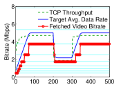
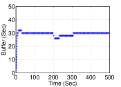
Figure 8: A PANDA client adapts its video bitrate under a bandwidth-varying link. The bandwidth is initially at 5 Mbps, drops to 2 Mbps at 200 seconds and rises back to 5 Mbps at 300 seconds.

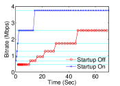
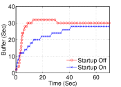
Figure 9: Comparison of the startup behavior of a PANDA player with and without the startup logic. The bandwidth is 5 Mbps.

The more intriguing question is whether PANDA could effectively stop the bitrate oscillation observed in the Smooth players. We conduct an experiment with the same setup as the experiment shown in Figure 1, except that the PANDA player and the Smooth player use slightly different video bitrate levels (due to different packaging methods). The resulting fetched bitrates in aggregate and for each client are shown in Figure 10. From the plot of the aggregate fetched bitrate, except for the initial fluctuation, the aggregate bitrate closely tracks the available bandwidth of 100 Mbps. Zooming in to the individual streams’ fetched bitrates, the fetched bitrates are confined within two adjacent bitrate levels and the number of shifts is much smaller than the Smooth client’s case. This affirms that PANDA is able to achieve better stability than the Smooth’s rate adaptation algorithm. In $\S$VI, we perform a comprehensive performance evaluation on each adaptation algorithm.

Fetched Bitrate Aggregated over 36 Streams

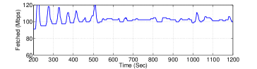
Fetched Bitrate of Individual Streams (Zoom In)

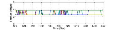
Figure 10: 36 PANDA clients compete at a 100-Mbps link in steady state.

To help the reader develop a better intuition on why PANDA performs better than a conventional algorithm, in Figure 11 we plot the trace of the measured TCP throughput and the target average data rate for the same experiment as in Figure 10. Note that the fair-share bandwidth for each client is about 2.8 Mbps. From the plot, the TCP throughput not only grossly overestimates the fair-share bandwidth, it also has a large variation. If used directly, this degree of noisiness gives the subsequent operations a very hard job to extract useful information. For example, one may apply strong filtering to smooth out the bandwidth measurement, but this would seriously affect the responsiveness of the client. When the network bandwidth suddenly drops, the client would not be able to respond quickly enough to reduce its video bitrate, leading to catastrophic buffer underrun. Moreover, the bias is both large and difficult to predict, making any correction to the mean problematic. In comparison, although also biased, the target average data rate estimated by the probing mechanism is much less noisy than the TCP throughput. One can easily correct the bias (via (15) and quantization) and select the right video bitrate without sacrificing responsiveness.

Measured TCP Throughput $\tilde{x}$

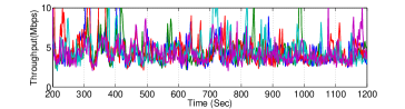
Target Average Data Rate $\hat{x}$

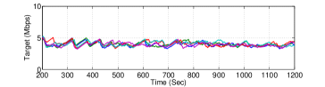
Figure 11: The traces of the TCP throughput and the target average data rate of 36 PANDA clients compete at a 100-Mbps link in steady state. The traces of the first five clients are plotted.

In Figure 12, we verify the stability criteria (13) and (14) of PANDA. With $\tau=2$, the system is stable if $\kappa<1$. This is demonstrated by Figure 12 (a), where we show the traces of the target average rate $\hat{x}$ for two $\kappa$ values 0.9 and 1.1. In Figure 12 (b), we show that when $\Delta=0$, the buffer cannot converge towards the reference level of 30 seconds.

VI Performance Evaluation

In this section, we conduct a set of test bed experiments to evaluate the performance of PANDA against other rate adaptation algorithms.

VI-A Evaluation Metrics

In $\S$V-A, we discussed four criteria that are most important for a user’s watching experience – i) ability to avoid buffer underruns, ii) quality smoothness, iii) average quality, and iv) fairness. In this paper, we use buffer undershoot as the metric for Criterion i), described as follows.

• Buffer undershoot: We measure how much the buffer goes down after a bandwidth drop as a indicator of an algorithm’s ability to avoid buffer underruns. The less the buffer undershoot, the less likely the buffer will underrun. Let $B_{o}$ be a reference buffer level (30 seconds for all players in this paper), and $B_{i,t}$ the buffer level for player $i$ at time $t$. The buffer undershoot for player $i$ at time $t$ is defined as $\frac{\max(0,B_{o}-B_{i,t})}{B_{o}}$. The buffer undershoot for player $i$ within a time interval $\mathcal{T}$ (right after a bandwidth drop), is defined as the 90th-percentile value of the distribution of buffer undershoot samples collected during $\mathcal{T}$.

We inherit the metrics defined in [13] – instability, inefficiency and unfairness, as the metrics for Criteria ii), iii) and iv), respectively. We only make a slight modification to the definition of inefficiency. Let $r_{i,t}$ be the video bitrate fetched by player $i$ at time $t$.

• Instability: The instability for player $i$ at time $t$ is $\frac{\sum_{d=0}^{k-1}|r_{i,t-d}-r_{i,t-d-1}|\cdot w(d)}{\sum_{d=0}^{k-1}r_{i,t-d}\cdot w(d)}$, where $w(d)=k-d$ is a weight function that puts more weight on more recent samples. $k$ is selected as 20 seconds.

• Inefficiency: Let $C$ be the available bandwidth. [13] defines inefficiency as $\frac{\left|\sum_{i}r_{i,t}-C\right|}{C}$ for player $i$ at time $t$. But sometimes the sum of fetched bitrate $\sum_{i}r_{i,t}$ can be greater than $C$. To avoid unnecessary penalty in this case, we revise the inefficiency metric to $\frac{\max\left(0,C-\sum_{i}r_{i,t}\right)}{C}$ for player $i$ at time $t$.

• Unfairness: Let $JainFair_{t}$ be the Jain fairness index calculated on the rates $r_{i,t}$ at time $t$ over all players. The unfairness at $t$ is defined as $\sqrt{1-JainFair_{t}}$.

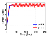
(a) $\kappa$

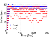
(b) $\Delta$

Figure 12: Experimental verification of PANDA’s stability criteria. In (a), one PANDA client streams over a link of 5 Mbps. In (b), 10 PANDA clients compete over a 10 Mbps link.

VI-B Experimental Setup

HAS Player Configuration: The benchmark players that we use to compare against PANDA are:

• Microsoft Smooth player [5], a commercially available proprietary player. The Smooth players are of version 1.0.837.34 using Silverlight runtime version 4.0.50826. To our best knowledge, the Smooth player as well as the Apple HLS and the Adobe HDS players all use the same TCP throughput measurement mechanism, so we picked the Smooth player as a representative.

• FESTIVE player, which we implemented based on the details specified in [13]. The FESTIVE algorithm is the first known client-side rate adaptation algorithm designed to specifically address the multi-client scenario.

• A player implementing the conventional algorithm (Algorithm 1), which differs from PANDA only in the estimating and scheduling steps.

For fairness, we ensure that PANDA and the conventional player use the same smoothing and quantizing functions. For smoothing, we implemented a EWMA smoother of the form: $\frac{\hat{y}[n]-\hat{y}[n-1]}{T[n-1]}=-\alpha\cdot\left(\hat{y}[n-1]-\hat{x}[n]\right)$, where $\alpha>0$ is the convergence rate of $\hat{y}[n]$ towards $\hat{x}[n]$. For quantization, we implemented a dead-zone quantizer $r[n]=Q(\hat{y}[n],r[n-1])$, defined as follows: Let the upshift threshold be defined as $r_{up}:=\begin{array}[]{ccc}\max_{r\in\mathcal{R}}r\end{array}$ subject to $r\leq\hat{y}[n]-\Delta_{up}$, and the downshift threshold as $r_{down}:=\begin{array}[]{ccc}\max_{r\in\mathcal{R}}r\end{array}$ subject to $r\leq\hat{y}[n]-\Delta_{down}$, where $\Delta_{up}$ and $\Delta_{down}$ are the upshift and downshift safety margin respectively, with $\Delta_{up}\geq\Delta_{down}\geq 0$. The dead-zone quantizer updates $r[n]$ as

$$r[n]=\begin{cases}r_{up},&r[n-1]<r_{up},\\ r[n-1],&r_{up}\leq r[n-1]\leq r_{down},\\ r_{down},&\mathrm{otherwise}.\end{cases}$$ (16)

The “dead zone” $[r_{up},r_{down}]$ created by setting $\Delta_{up}>\Delta_{down}$ mitigates frequent bitrate hopping between two adjacent levels, thus stabilizing the video quality (i.e. hysteresis control). For the conventional player, set $\Delta_{up}=\epsilon\cdot\hat{y}$ and $\Delta_{down}=0$, where $0\leq\epsilon<1$ is the multiplicative safety margin. For PANDA, due to (14) and (15), set $\Delta_{up}=w+\epsilon\cdot\hat{y}$ and $\Delta_{down}=w$ .

Table II lists the default parameters used by each player, as well as their varying values. For fairness, all players attempt to maintain a steady-state buffer of 30 seconds. For PANDA, $B_{\min}$ is selected to be 26 seconds such that the resulting steady-state buffer is 30 seconds (by (12)).

Server Configuration: The HTTP server runs Apache on Red Hat 6.2 (kernel version 2.6.32-220). The Smooth player interacts with an Microsoft IIS server by default, but we also perform experiments of Smooth player interacting with an Apache server on Ubuntu 10.04 (kernel version 2.6.32.21).

Network Configuration: As service provider deployment over a managed network is our primary case of interest, our experiments are configured to highly match the imporant scenario where a number of HAS flows compete for bandwidth within a DOCSIS bonding group. The test bed is configured as in Figure 13. The queueing policy used at the aggregation router-home router bottleneck link is the following. For a link bandwidth of 10 Mbps or below, we use random early detection (RED) with $(min\_thr,max\_thr,p)=(30,90,0.25)$; if the link bandwidth is 100 Mbps, we use RED with $(min\_thr,max\_thr,p)=(300,900,1)$. The video content is chopped into segments of $\tau=2$ seconds, pre-encoded with $L=10$ bitrates: 459, 693, 937, 1270, 1745, 2536, 3758, 5379, 7861 and 11321 Kbps. For the Smooth player, the data rates after packaging are slightly different.

Algorithm	Parameter	Default	Values
PANDA	$\kappa$	0.14	0.04,0.07,0.14,0.28,0.42,0.56
	$w$	0.3
	$\alpha$	0.2	0.05,0.1,0.2,0.3,0.4,0.5
	$\beta$	0.2
	$\epsilon$	0.15	0.5,0.4,0.3,0.2,0.1,0
	$B_{\min}$	26
Conventional	$\alpha$	0.2	0.01,0.04,0.07,0.1,0.15,0.2
	$\epsilon$	0.15
	$B_{\max}$	30
FESTIVE	Window	20	20,15,10,6,3,1
	$targetbuf$	30

TABLE II: Parameters used in experiments

Figure 13: The network topology configured in the test bed. Local indicates that the bitrate is effectively unbounded and the link delay is 0 ms.

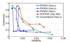
(a)

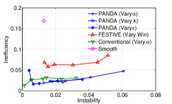
(b)

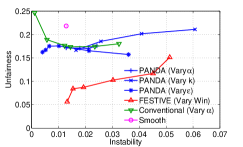
(c)

Figure 14: The impact of varying instability on buffer undershoot, inefficiency and unfairness for PANDA and other benchmark players.

VI-C Performance Tradeoffs

It would not be legitimate to discuss a single metric without minding its impact on other metrics. In this section, we examine the performance tradeoffs among the four metrics of interest. We designed an experimental process under which we can measure all four metrics in a single run. For each run, five players (of the same type) compete at a bottleneck link. The link bandwidth stays at 10 Mbps from 0 seconds to 400 seconds, drops to 2.5 Mbps at 400 seconds and stays there until 500 seconds. We record the instability, inefficiency and unfairness averaged over 0 to 400 seconds over all players, and the buffer undershoot over 400 to 500 seconds averaged over all players. Figure 14 shows the tradeoff between stability and each of the other criteria – buffer undershoot, inefficiency and unfairness – for each of the types of player. Each data point is obtained via averaging over 10 runs, and each data point represents a different value for one of the parameters of the corresponding algorithm, as indicated in the Values column of Table II.

For the PANDA player, the three parameters that affect instability the most are: the probing convergence rate $\kappa$, the smoothing convergence rate $\alpha$ and the safety margin $\epsilon$. Figure 14 (a) shows that as we vary these parameters, the tradeoff curves mostly stay flat (except for at extreme values of these parameters), implying that the PANDA player maintains good responsiveness as the stability is improved. A few factors contribute to this advantage of PANDA: First, as the bandwidth estimation by probing is quite accurate, one does not need to apply strong smoothing. Second, since after a bandwidth drop, the video bitrate reduction is made proportional to the TCP throughput reduction, PANDA is very agile to bandwidth drops. On the other hand, for both the FESTIVE and the conventional players, the buffer undershoot significantly increases as the scheme becomes more stable. Overall, PANDA has the best tradeoff between stability and responsiveness to bandwidth drop, outperforming the second best conventional player by more than 75% reduction in instability at the same buffer undershoot level. It is worth noting that the conventional player uses exactly the same smoothing and quantization steps as PANDA, which implies that the gain achieved by PANDA is purely due to the improvement in the estimating and scheduling steps. FESTIVE has the largest buffer undershoot. We believe this is because the design of FESTIVE has mainly concentrated on stability, efficiency and fairness, but ignored responsiveness to bandwidth drops. As we do not have access to the Smooth player’s buffer, we do not have its buffer undershoot measure in Figure 14 (a).

Figure 14 (b) shows that PANDA has the lowest inefficiency over all as we vary its instability. The probing mechanism ensures that the bandwidth is most efficiently utilized. As the instability increases, the inefficiency also increases moderately. This makes sense intuitively, as when the bitrate fluctuates, the average fetched bitrate also decreases. The efficiency of the conventional algorithm underperforms PANDA, but outperforms FESTIVE. Lastly, the Smooth player has the highest inefficiency.

Lastly, Figure 14 (c) shows that in terms of fairness, FESTIVE achieves the best performance. This may be due to the randomized scheduling strategy of FESTIVE. PANDA and the conventional players have similar fairness; both of them outperform the Smooth player.

VI-D Increasing Number of Players

In this section, we focus on the question of how the number of players affects instability, inefficiency and unfairness at steady state. Two scenarios are of interest: i) we increase the number of players while fixing the link bandwidth at 10 Mbps, and ii) we increase the number of players while varying the bandwidth such that the bandwidth/player ratio is fixed at 1 Mbps/player. Figure 15 and Figure 16 report results for these two cases, respectively. Each data point is obtained by averaging over 10 runs.

Refer to Figure 15 (a). In the single-player case, all four schemes are able to maintain their fetched video bitrate at a constant level, resulting in zero instability. As the number of players increases, the instability of the conventional player and the Smooth player both increase quickly in a highly consistent way. We speculate that they have very similar underlying structure. The FESTIVE player is able to maintain its stability at a lower level, due to the strong smoothing effect (smoothing window at 20 samples by default), but the instability still grows with the number of players, likely due to the bandwidth overestimation effect. The PANDA player exhibits a rather different behavior: at two players it has the highest instability, then the instability starts to drop as the number of players increases. Investigating into the experimental traces reveals that this is related to the specific bitrate levels selected. More importantly, via probing, the PANDA player is immune to the symptoms of the bandwidth overestimation, thus it is able to maintain its stability as the number of clients increases. The case of varying bandwidth in Figure 16 (a) exhibits behavior fairly consistent with Figure 15 (a), with PANDA and FESTIVE exhibiting much less instability compared to the Smooth and the conventional players.

Figure 15 (b) and Figure 16 (b) for the inefficiency metric both show that PANDA consistently has the best performance as the number of players grow. The conventional player and FESTIVE have similar performance, both outperforming the Smooth player by a great margin. We speculate that the Smooth player has some large bitrate safety margin by design, with the purpose of giving cross traffic more breathing room.

Lastly, let us look at fairness. Refer to Figure 15 (a). We have found that when the overall bandwidth is fixed, the unfairness measure has high dependence on the specific bitrate levels chosen, especially when the number of players is small. For example, at two players, when the fair-share bandwidth is 5 Mbps, the two PANDA players end up in steady state with 5.3 Mbps and 3.7 Mbps, resulting in a high unfairness score. At three players, when the fair-share bandwidth is 3.3 Mbps, the three PANDA players each end up with 3.7, 3.7 and 2.5 Mbps for a long period of time, resulting in a lower unfairness score. FESTIVE exhibits lowest unfairness overall, which is consistent with the results obtained in Figure 14 (c). In the varying-bandwidth case in Figure 16 (c), The unfairness ranking is fairly consistent as the number of players grow: FESTIVE, PANDA, the conventional, and Smooth.

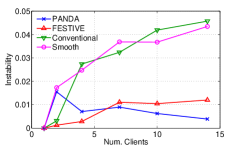
(a)

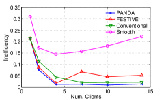
(b)

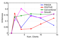
(c)

Figure 15: Instability, inefficiency and unfairness as the number of clients increases. The link bandwidth is fixed at 10 Mbps.

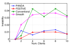
(a)

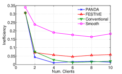
(b)

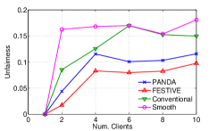
(c)

Figure 16: Instability, inefficiency and unfairness as the number of clients increases. The link bandwidth increases with the number of players, with the bandwidth-player ratio fixed at 1 Mbps/player.

VI-E Competing Mixed Players

One important question to ask is how PANDA will behave in the presence of different type of players? If it behaves too conservatively and cannot grab enough bandwidth, then the deployment of PANDA will not be successful. To answer this question, we take the four types of players of interest and have them compete on a 10-Mbps link. For the Smooth player, we test it with both a Microsoft IIS server running on Windows 7, and an Apache HTTP server running on Ubuntu 10.04. A single trace of the fetched bitrates for 500 seconds is shown in Figure 17. The plot shows that the Smooth player’s ability to grab the bandwidth highly depends on the server it streams from. Using the IIS server, which runs on Windows 7 with an aggressive TCP, it is able to fetch video bitrates over 3 Mbps. With the Apache HTTP server, which uses Ubuntu 10.04’s conservative TCP, the fetched bitrates are about 1 Mbps. The conventional, PANDA and FESTIVE players all run on the same TCP (Red Hat 6), so their differences are due to their adaptation algorithms. Due to bandwidth overestimation, the conventional player aggressively fetches high bitrates, but the fetched bitrates fluctuate. Both PANDA and FESTIVE are able to maintain a stable fetched bitrate at about the fair-share level of 2 Mbps.

VI-F Summary of Performance Results

• The PANDA player has the best stability-responsiveness tradeoff, outperforming the second best conventional player by 75% reduction in instability. PANDA also has the best bandwidth utilization.

• The FESTIVE player has been tuned to yield high stability, high efficiency and good fairness. However, it underperforms other players in responsiveness to bandwidth drops.

• The conventional player yields good efficiency, but lacks in stability, responsiveness to bandwidth drops and fairness.

• The Smooth player underperforms in efficiency, stability and fairness. When competing against other players, its ability to grab bandwidth is a consequence of the aggressiveness of the underlying TCP stack.

VII Related Work

AIMD Principle: The design of the probing mechanism in PANDA shares similarity with Jacobson’s AIMD principle for TCP congestion control [11]. Kelly’s framework on network rate control [14] provides a theoretical justification for the AIMD principle, and proves its stability in the general network setup.

HAS Measurement Studies: Various research efforts have focused on understanding the behavior of several commercially deployed HAS systems. One such example is [2], where the authors characterize and evaluate HTTP streaming players such as Microsoft Smooth Streaming, Netflix, and Adobe OSMF via experiments in controlled settings. The first measurement study to consider HAS streaming in the multi-client scenarios is [3]. The authors identify the root cause of the player’s rate oscillation problem as the existence of on-off patterns in HAS traffic. In [10], the authors measure behavior of commercial video streaming services, i.e., Hulu, Netflix, and Vudu, when competing with other long-lived TCP flows. The results revealed that inaccurate estimations can trigger a feedback loop leading to undesirably low-quality video.

Existing HAS Designs: To improve the performance of adaptive HTTP streaming, several rate adaptation algorithms [15, 19, 20, 17, 16] have been proposed, which, in general, fit into the four-step model discussed in Section II-B. In [12], a sophisticated Markov Decision Process (MDP) is employed to compute a set of optimal client strategies in order to maximize viewing quality. The MDP requires the knowledge of network conditions and video content statistics, which may not be readily available. Control-theoretical approaches, including use of a PID controller, are also considered by several works [6, 19, 20]. A PID controller with appropriate parameter choice can improve streaming performance. Server-side mechanisms are also advocated by some works [9, 4]. Two designs have been considered to address the multi-client issues: in [4], a rate-shaping approach aiming to eliminate the off-intervals, and in [13], a client rate adaptation algorithm design implementing a combination of randomization, stateful rate selection and harmonic mean based averaging.

VIII Conclusions

This paper identifies an emerging issue for HTTP adaptive streaming, which is expected to become the predominant form of the Internet traffic, and lays out a solution direction that can effectively address this issue. Our main contributions in this paper can be summarized as follows:

• We have identified the bandwidth cliff effect as the root cause of the bitrate oscillation phenomenon and revealed the fundamental limitation of the conventional reactive measurement based rate adaptation algorithms.

• We have envisioned a general probe-and-adapt principle to directly address the root cause of the problems, and designed and implemented PANDA, a client-based rate adaptation algorithm, as an embodiment of this principle.

• We have proposed a generic four-step model for an HAS rate adaptation algorithm, based on which we have fairly compared the proposed approach with the conventional approach.

The probe-and-adapt approach and our PANDA realization thereof achieve significant improvements in stability of HAS systems at no cost in responsiveness. Given this framework, we plan to explore further improvements in our future work.

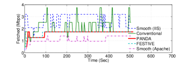
Figure 17: PANDA, Smooth (w/ IIS), Smooth (w/ Apache), FESTIVE and the conventional players compete at a bottleneck link of 10 Mbps.

Appendix A Bandwidth Cliff Effect: Theoretical Analysis

A-A Problem Formulation

Consider that $K$ clients share a bottleneck link of capacity $C$. The streaming process of each client consists of discrete downloading steps $n=1,2,...$, where during each step one video segment is downloaded.

Fixed requested video bitrate. As we are interested in how the measured TCP throughput causes HAS clients to shift their video bitrates requested, we analyze the stage of the dynamics where the rate shift has not occurred yet. Thus, in our model, we assume that each HAS client does not change its requested video bitrate over the time interval of analysis. For $k=1,...K$, each $k$-th client requests a video segment of fixed size $r_{k}\cdot\tau$ at each downloading step, where $r_{k}\in\mathcal{R}$ is the video bitrate selected.

Segment requesting time and downloading duration. Denote by $R_{k}(t)$ the instantaneous data downloading rate of the $k$-th client at time $t$ (note that $R_{k}$ and $r_{k}$ are different). Denote by $t_{k}[n]$ the time that the $k$-th client requests its $n$-th segment (which, for simplicity, is also assumed to be the time that the downloading starts). For each client, assume that the requesting time of the first segment $t_{k}[1]$ is given. For $n\geq 1$, the requesting time of the next segment is determined by:

$$t_{k}[n+1]=t_{k}[n]+\max(\tau,\tilde{T_{k}}[n]),$$ (17)

where $\tilde{T_{k}}[n]$ is the actual duration of the $k$-th client downloading its $n$-th segment. This is a reasonable assumption where the buffer level of a HAS client has reached the maximum level. The actual duration of downloading, $\tilde{T_{k}}[n]$, can be related to $r_{k}$ by

$$\int_{t=t_{k}[n]}^{t_{k}[n]+\tilde{T_{k}}[n]}R_{k}(t)\cdot dt=r_{k}\cdot\tau.$$ (18)

The TCP throughput measured by the $k$-th client for downloading the $n$-th segment, is defined as $\tilde{x}_{k}[n]:=\frac{r_{k}\cdot\tau}{\tilde{T_{k}}[n]}$. In a conventional HAS algorithm, the TCP throughput is used as an estimator of a client’s fair-share bandwidth, which, ideally, is equal to $\frac{C}{K}$.

Idealized TCP behavior. We assume that the network obeys a simplified bandwidth sharing model, where we do not consider the effects such as TCP slow-start restart and heterogenous RTTs. At any moment $t\geq 0$ when there are $A(t)\geq 1$ active TCP flows sharing the bottleneck link, each active flow will receive a fair-share data rate of $R_{k}(t)=\frac{C}{A(t)}$ instantaneously, and the total traffic rate in the link is $C$; at any moment when there is no active TCP flows, or $A(t)=0$, the total traffic rate in the link is $0$. For this case, we have the following definition:

Definition 1.

A gap is an interval within which the total traffic rate of all clients is $0$.

Client initial state. We assume that each client may have some arbitrary initial state, including:

• Time of requesting the first segment $t_{k}[1]$, $k=1,...,K$, as forementioned.

• Initial data downloading rate, i.e., it may be that $R_{k}(t)>0$ for $t<t_{k}[1]$, $k=1,...,K$, where the rate may be due to requesting a segment earlier than the first segment being considered. In practice, this may correspond to the cases where the clients have already started downloading but may be in a different state, before the first segment being considered (e.g., link is oversubscribed before it becomes undersubscribed).

A-B Link Undersubscription

The link is undersubscribed by the $K$ HAS clients if the sum of the requested video bitrates is less than the link capacity, i.e., $\sum_{k=1}^{K}r_{k}<C$. We would like to show that even the slightest undersubscription of the link would lead to convergence into a state where each client has a TCP throughput greater than its fair-share bandwidth $\frac{C}{K}$.

To begin with, we prove a set of lemmas. We first show that any two adjacent requesting times $t_{k}[n]$ and $t_{k}[n+1]$ are spaced by exactly $\tau$ if there exists a gap between them.

Lemma 2.

$t_{k}[n+1]=t_{k}[n]+\tau$ if there exists a gap $[t^{-},t^{+})$ with $t_{k}[n]\leq t^{-}$ and $t^{+}\leq t_{k}[n+1]$.

Proof:

By (17), the only case that $t_{k}[n+1]\neq t_{k}[n]+\tau$ is when $\tilde{T_{k}}[n]>\tau$. But this cannot hold, since otherwise there cannot be a gap $[t^{-},t^{+})$ with $t_{k}[n]\leq t^{-}$ and $t^{+}\leq t_{k}[n+1]$. ∎

The rest of the lemmas in this section make the assumption of $\sum_{k=1}^{K}r_{k}<C$. First, we show that at least one gap must emerge after some time.

Lemma 3.

There exists a gap $[t^{-},t^{+})$, where $t^{-}>\max_{k}t_{k}[1]$.

Proof:

By (17), within $[t,t+\tau)$ for any $t$, each client can download at most one segment, or data of size at most $r_{k}\cdot\tau$. Consider within an interval $[\max_{k}t_{k[1]},\max_{k}t_{k[1]}+m\cdot\tau)$ for some $m\in\mathcal{N}$. The maximum size of the data that can be downloaded by the $K$ clients is $B_{res}+m\cdot\sum_{k=1}^{K}r_{k}\tau$, where $B_{res}$ is the total size of the residue data from segments requested prior to $\max_{k}t_{k}[1]$, including those prior to the first segments being considered, as discussed in Section A-A, client initial state. By the idealized TCP behavior, at any instant, the total traffic rate can be either $C$ or $0$. If zero total traffic rate does not happen, the total downloaded data size within the interval being considerd is $mC\tau$. Therefore, a sufficient condition for a gap $[t^{-},t^{+})$ to occur is to have $t^{-}>\max_{k}t_{k[1]}+m\cdot\tau$, where $mC\tau>B_{res}+m\cdot\sum_{k=1}^{K}r_{k}\tau$, or $m=\left\lceil B_{res}/\tau\cdot(C-\sum_{k=1}^{K}r_{k})\right\rceil$. ∎

The next lemma shows that within an interval of duration $\tau$ immediately following this gap, each client must request one and only one segment.

Lemma 4.

Within the interval $[t^{+},t^{+}+\tau)$, each client must request one and only one segment.

Proof:

First, we show that each client must request at least one segment. Invoking Lemma 2 and the fact that $[t^{-},t^{+})$ is a gap, the request times immediately preceding and following $[t^{-},t^{+})$ must be spaced exactly by $\tau$. This can never hold if no segment is requested within $[t^{+},t^{+}+\tau)$.

Second, we show that each client can request at most one segment within $[t^{+},t^{+}+\tau)$. This directly follows applying (17) to any interval of duration $\tau$, similar to the proof of Lemma 3. ∎

Since exactly one segment is requested by each client within $[t^{+},t^{+}+\tau)$, for convenience, let us re-label these segments using a new index $n^{\prime}$.

Lemma 5.

$[t^{-}+\tau,t^{+}+\tau)$ is a gap.

Proof:

First, invoking Lemma 2 and the fact that $[t^{-},t^{+})$ is a gap, we have $t_{k}[n^{\prime}-1]=t_{k}[n^{\prime}]-\tau$ for $k=1,...,K$. In other words, the starting time patterns within intervals $[t^{+}-\tau,t^{+})$ and $[t^{+},t^{+}+\tau)$ exactly repeat.

Second, consider the data traffic within $[t^{+}-\tau,t^{+})$ and $[t^{+},t^{+}+\tau)$. The only difference is that within $[t^{+}-\tau,t^{+})$, there might be unfinished residue data from the previous segments whereas within $[t^{+},t^{+}+\tau)$, there is no such unfinished residue data due to the gap $[t^{-},t^{+})$. By (18), the exact starting times and the idealized TCP behavior, the downloading completion time can only get delayed with the extra residue data, thus we must have $\tilde{T}_{k}[n^{\prime}-1]\geq\tilde{T}_{k}[n^{\prime}]$, $k=1,...,K$. Therefore, the data traffic within $[t^{+},t^{+}+\tau)$ must finish no later than $t^{-}+\tau$, and $[t^{-}+\tau,t^{+}+\tau)$ must also be a gap. ∎

The following theorem shows that in the case of link undersubscription, regardless of the client initial states, the banwidth sharing among the clients will eventually converge to a periodic pattern.

Theorem 6.

If $\sum_{k=1}^{K}r_{k}<C$, the data downloading rate $R_{k}(t)$ of each client will converge to a periodic pattern with period $\tau$, i.e., there exists some $t^{\prime}\geq 0$ such that for all $t\geq t^{\prime}$, $R_{k}(t+\tau)=R_{k}(t)$, $k=1,...,K$.

Proof:

The interval $[t^{+},t^{+}+\tau)$ has no residue data from the previous unfinished segments, because of the gap $[t^{-},t^{+})$. Using this fact and the idealized TCP behavior, the data downloading rates $R_{k}(t)$, $k=1,...,K$ for $t\in[t^{+},t^{+}+\tau)$ is a deterministic function of the starting times $t_{k}[n^{\prime}]$, $k=1,...,K$. The same argument applies to $R_{k}(t)$, $k=1,...,K$ for $t\in[t^{+}+\tau,t^{+}+2\tau)$ and $t_{k}[n^{\prime}+1]$, $k=1,...,K$.

By Lemma 2 and Lemma 5, we have $t_{k}[n^{\prime}+1]=t_{k}[n^{\prime}]+\tau$ for $k=1,...,K$. In other words, other than the offset $\tau$, the starting time patterns within $[t^{+},t^{+}+\tau)$ and $[t^{+}+\tau,t^{+}+2\tau)$ are the same. Invoking the deterministic function argument, we can show $R_{k}(t+\tau)=R_{k}(t)$, $k=1,...,K$ for $t\in[t^{+},t^{+}+\tau)$. Taking $t^{\prime}=t^{+}$ and repeatly applying the argument above to the intervals $[t^{+}+m\tau,t^{+}+(m+1)\tau)$, $m=2,3,...$ complete the proof. ∎

Note that by the idealized TCP behavior, no client’s TCP throughput would overestimate its fair-share bandwdith $\frac{C}{K}$ only if the number of active flows $A(t)=K$ during all the active time. After the bandwith sharing pattern converges to periodic, this happens only when the starting times of all clients are all aligned and their segment data size are equal. The following corollary is an immediate consequence of Theorem 6:

Corollary 7.

If $\sum_{k=1}^{K}r_{k}<C$, and $t_{k}[n^{\prime}]\neq t_{l}[n^{\prime}]$ for some $k\neq l$, then for some clients the TCP throughput will converge to a value that is greater than its fair-share bandwdith, i.e., there exists $k^{\prime}$ with $\tilde{x}_{k^{\prime}}[n]>\frac{C}{K}$ for $n\geq n^{\prime}$. In particular, if $r_{1}=r_{2}=...=r_{K}$, then for all $k^{\prime}=1,...,K$, $\tilde{x}_{k^{\prime}}[n]>\frac{C}{K}$ for $n\geq n^{\prime}$.

Note that the start times pattern $t_{k}[n^{\prime}]$, $k=1,...,K$ will dictate exactly by how much the TCP throughput overestimates the fair-share bandwidth, with the range $\frac{\tilde{x}_{k}[n]}{C/K}\in[1,K]$.

A-C Link Oversubscription

We next consider the case that the link is oversubscribed by the $K$ HAS clients, i.e., $\sum_{k=1}^{K}r_{k}>C$. We first show a sufficient condition under which the TCP throughput would correctly predict the fair-share bandwidth.

Theorem 8.

If $r_{k}>\frac{C}{K}$ for all $k=1,...,K$, all clients’ TCP throughput converges to the fair-share bandwidth, i.e., there exists $n^{\prime}>0$ such that $\tilde{x}_{k}[n]=\frac{C}{K}$, $k=1,...,K$ for $n\geq n^{\prime}$.

Proof:

We first want to show that there exists $n^{\prime}>0$ such that $\tilde{T}_{k}[n]>\tau$ for all $k=1,...,K$ for $n\geq n^{\prime}$. Assume that the opposite is true, i.e., there exists at least a client $k^{\prime}$ such that, $\tilde{T}_{k^{\prime}}[n]\leq\tau$ for all $n\geq n^{\prime}$. Since $r_{k^{\prime}}>\frac{C}{K}$, this would hold only if within the active intervals of client $k^{\prime}$, at least another client $k^{\prime\prime}$ must be inactive. Denote by $[t_{k^{\prime\prime}}^{-},t_{k^{\prime\prime}}^{+})$ the first such inactive interval. Consider within an interval $[t_{k^{\prime\prime}}^{-},t_{k^{\prime\prime}}^{-}+m\cdot\tau)$ for some $m\in\mathcal{N}$. By the idealistic TCP behavior, the total number of bits that can be downloaded by the $K-1$ clients (other than $k^{\prime}$) must be $\leq(K-1)/K\cdot m\tau C$. This contradicts the fact that $\tilde{T}_{k}[n]>\tau$, for $k\neq k^{\prime}$, $n\geq n^{\prime}$. Thus, the assumption is invalid.

Then, by (17), for $n\geq n^{\prime}$, all clients are active all the time. By the idealistic TCP behavior, we have $\tilde{x}_{k}[n]=\frac{C}{K}$, $k=1,...,K$ for $n\geq n^{\prime}$. ∎

By slightly extending the above argument, a sufficient and necessary condition for the correct fair-share bandwidth estimation of all clients can be found.

Theorem 9.

If $\sum_{k=1}^{K}r_{k}>C$, all clients’ TCP throughput converges to the fair-share bandwidth, if and only if $r_{k}\geq\frac{C}{K}$ for all $k=1,...,K$ and there exists $k^{\prime}$ such that $r_{k^{\prime}}>\frac{C}{K}$.

Appendix B Analysis of PANDA

We perform an equilibrium and stability analysis of PANDA. For simplicity, we only analyze the single-client case where the system has an equilibrium point.

B-A Analysis of $\hat{x}$

Assume the measured TCP download throughput $\tilde{x}$ is equal to the link capacity $C$. Consequently, (7) can be re-written in two scenarios (refer to Figure 3) as:

$$\frac{\hat{x}[n]-\hat{x}[n-1]}{T[n-1]}=\begin{cases}\kappa\cdot w,&\mbox{if~{}}\hat{x}<C,\\ \kappa\cdot w-\kappa\cdot(\hat{x}[n-1]-C),&\mbox{otherwise}.\end{cases}$$ (19)

At equilibrium, setting (19) to zero leads to $w=\hat{x}_{o}-C$, hence, $\hat{x}_{o}=C+w>\tilde{x}_{o}=C$.

Considering the simplifying assumptions of $\hat{y}=\hat{x}$ (no smoothing) and a quantizer with a margin $\Delta$ such that $r=\hat{y}-\Delta$, we need $r_{o}=\hat{x}_{o}-\mbox{$\Delta$}<C$ at equilibrium. Therefore, the quantization margin of the quantizer needs to satisfy

$$\Delta>\hat{x}_{o}-C=w,$$

so that the system stays on the multiplicative-decrease side of the equation at steady state.

Note that close to equilibrium, the intervals between consecutive segment downloads match the segment playout duration $T[n-1]=\tau$, therefore, calculation of the estimated bandwidth $\hat{x}$ follows the simple form of a difference equation:

$$\hat{x}[n]=a\cdot\hat{x}[n-1]+b.$$

The two constants are: $a=1-\kappa\cdot\tau$ and $b=\kappa\cdot(C+w)\cdot\tau$. The sequence converges if and only if $|a|<1$. Hence, we need: $-1<1-\kappa\cdot\tau<1$, leading to the stability criterion:

$$0<k<\frac{2}{\tau}.$$

B-B Analysis of $\hat{T}$ and $B$

Assume no smoothing $\hat{x}=\hat{y}$. During transient states, when $T=\hat{T}>\tilde{T}$, update of $\hat{T}$ pushes the playout buffer size in the right direction: $\hat{T}<\frac{r[n]\cdot\tau}{\hat{x}[n]}$ leads to a steady growth in buffer size when $B<B_{\min}$. At steady state, $\hat{T}_{o}=\tau=\hat{T}_{o}>\tilde{T}_{o}$. It can be derived from (10) that:

$$B_{o}=B_{\min}+\left(1-\frac{r_{o}}{\hat{x}_{o}}\right)\cdot\frac{\tau}{\beta}$$

where $B_{o}$ is playout buffer at equilibrium.

References

- [1] History of Move Networks. Available online: http://www.movenetworks.com/history.html.
- [2] S. Akhshabi, S. Narayanaswamy, Ali C. Begen, and C. Dovrolis. An experimental evaluation of rate-adaptive video players over HTTP. Signal Processing: Image Communication, 27:271–287, 2012.
- [3] Saamer Akhshabi, Lakshmi Anantakrishnan, Constantine Dovrolis, and Ali C. Begen. What happens when HTTP adaptive streaming players compete for bandwidth. In Proc. ACM Workshop on Network and Operating System Support for Digital Audio and Video (NOSSDAV’12), Toronto, Ontario, Canada, 2012.
- [4] Saamer Akhshabi, Lakshmi Anantakrishnan, Constantine Dovrolis, and Ali C. Begen. Server-based traffic shaping for stabilizing oscillating adaptive streaming players. In to appear in NOSSDAV13, 2013.
- [5] Alex Zambelli. IIS Smooth Streaming Technical Overview. http://tinyurl.com/smoothstreaming.
- [6] Luca De Cicco, Saverio Mascolo, and Vittorio Palmisano. Feedback control for adaptive live video streaming. In Proc. ACM Multimedia Systems Conference (MMSys’11), pages 145–156, San Jose, CA, USA, February 2011.
- [7] Cisco White Paper. Cisco visual networking index - forecast and methodology, 2011-2016. http://tinyurl.com/ciscovni2011to2016.
- [8] F. Dobrian, V. Sekar, A. Awan, I. Stoica, D. Joseph, A. Ganjam, J. Zhan, and H. Zhang. Understanding the impact of video quality on user engagement. In Proceedings of the ACM SIGCOMM 2011 conference, SIGCOMM ’11, pages 362–373, New York, NY, USA, 2011. ACM.
- [9] Remi Houdaille and Stephane Gouache. Shaping http adaptive streams for a better user experience. In Proceedings of the 3rd Multimedia Systems Conference, pages 1–9, 2012.
- [10] Te-Yuan Huang, Nikhil Handigol, Brandon Heller, Nick McKeown, and Ramesh Johari. Confused, timid, and unstable: Picking a video streaming rate is hard. In Proceedings of the 2012 ACM conference on Internet measurement conference, 2012.
- [11] V. Jacobson. Congestion avoidance and control. In Symposium proceedings on Communications architectures and protocols, SIGCOMM ’88, pages 314–329, New York, NY, USA, 1988. ACM.
- [12] Dmitri Jarnikov and Tanir Ozcelebi. Client Intelligence for Adaptive Streaming Solutions. EURASIP Journal on Signal Processing: Image Communication, Special Issue on Advances in IPTV Technologies, 26(7):378–389, August 2011.
- [13] Junchen Jiang, Vyas Sekar, and Hui Zhang. Improving fairness, efficiency, and stability in http-based adaptive video streaming with festive. In Proceedings of the 8th international conference on Emerging networking experiments and technologies (CoNEXT), 2012.
- [14] F. P. Kelly, A. K. Maulloo, and D. K. H. Tan. Rate control for communication networks: Shadow prices, proportional fairness and stability. The Journal of the Operational Research Society, 49(3):237–252, 1998.
- [15] Chenghao Liu, Imed Bouazizi, and Moncef Gabbouj. Rate Adaptation for Adaptiv HTTP streaming. In Proc. ACM Multimedia Systems Conference (MMSys’11), pages 169–174, San Jose, CA, USA, February 2011.
- [16] Chenghao Liu, Imed Bouazizi, Miska M. Hannuksela, and Moncef Gabbouj. Rate adaptation for dynamic adaptive streaming over HTTP in content distribution network. Signal Processing: Image Communication, 27(4):288–311, April 2012.
- [17] Konstantin Miller, Emanuele Quacchio, Gianluca Gennari, and Adam Wolisz. Adaptation algorithm for adaptive streaming over http. In Proceedings of 2012 IEEE 19th International Packet Video Workshop, pages 173–178, 2012.
- [18] R.K.P. Mok, E.W.W. Chan, X. Luo, and R.K.C. Chang. Inferring the QoE of HTTP video streaming from user-viewing activities. In Proc. SIGCOMM W-MUST, 2011.
- [19] Guibin Tian and Yong Liu. Towards agile and smooth video adaptation in dynamic http streaming. In Proceedings of the 8th international conference on Emerging networking experiments and technologies (CoNEXT), pages 109–120, 2012.
- [20] Chao Zhou, Xinggong Zhang, Longshe Huo, and Zongming Guo. A control-theoretic approach to rate adaptation for dynamic http streaming. In Proceedings of Visual Communications and Image Processing (VCIP), pages 1–6, 2012.