Real time evolution at finite temperatures with operator space matrix product states

Abstract

We propose a method to simulate the real time evolution of one dimensional quantum many-body systems at finite temperature by expressing both the density matrices and the observables as matrix product states. This allows the calculation of expectation values and correlation functions as scalar products in operator space. The simulations of density matrices in inverse temperature and the local operators in the Heisenberg picture are independent and result in a grid of expectation values for all intermediate temperatures and times. Simulations can be performed using real arithmetics with only polynomial growth of computational resources in inverse temperature and time for integrable systems. The method is illustrated for the XXZ model and the single impurity Anderson model.

1 Introduction

The simulation of strongly interacting quantum many-body systems is, in general, a computationally difficult task. Even in the case of one-dimensional quantum systems with finite range interactions, where ground state properties have become readily accessible using the density matrix renormalization group (DMRG) algorithm [1], accessing the dynamics remains hard. While, the matrix product states (MPS) [2, 3, 4] that are at the core of DMRG manage to describe the ground states due to their weak entanglement [5, 6], the entanglement increases in the real time evolution [3, 5, 7, 8] making the study of dynamics computationally challenging even for pure states.

Even harder is dynamics at finite temperatures. MPS based methods operate on the level of wave functions. Systems at thermal equilibrium, described by a mixture of quantum states, thus need to be purified by being described as a pure state in an enlarged system, consisting of the system and an auxiliary environment. The simulation is then performed on this purified system [4, 9] and by tracing over the degrees of freedom of the environment, the properties of the original system are obtained. This idea was first implemented in Ref. [4, 10] for density matrices of thermal quantum systems and systems far from equilibrium. The same concept was used in the simulation of dynamical properties of thermal systems where the real time evolution was computed on the level of the purified system and the density operator for the original system was obtained by tracing over the environment [11, 12].

A disadvantage of these purification based approaches is that they require additional information on the environment, and especially on its dynamics. In general, these methods are accompanied by an exponential growth of computational resources with time and elaborate procedures are required to control the fast growth of entanglement. Recent advances in the application to the XXZ model have shown that a smart choice of the environmental dynamics can significantly extend the accessible simulation times [13]. However, the question of the optimal environment and its dynamics is still open. Even finding a good choice of the environmental dynamics requires deep knowledge of the system and is far from being straightforward.

Here we propose an alternative strategy, based on operator space concepts and matrix product states. Similarly to the purification approach, we describe the density matrices as many-body states; however, our states are not superpositions of quantum states but superpositions of operators [14, 10]. In the same way we also describe the observables and their dynamics, known as the time dependent DMRG in the Heisenberg picture [14, 15]. An operator space approach was used in [16], however, still retaining the exponential growth of computational costs. The key feature of our approach is the combination of both concepts where the expectation value of an observable at a given time and temperature is calculated as a scalar product of two vectors in the operator space, one representing the density matrix and the other the real time evolution of an operator. This way, the simulation of density matrices and the real time evolution of operators are decoupled and can be performed independently such that only two simulations are sufficient to calculate a grid of expectation values at various intermediate (inverse) temperatures and times.

The computational costs to simulate the density matrices grow polynomially in time due to a low degree of correlation at thermal equilibrium [17], although such description has mostly been used to simulate systems far from the equilibrium [18]. Similarly, the simulation of local operators also exhibits polynomial growth of resources [14] for integrable systems. This corresponds to a logarithmic growth of the operator space equivalent of the entanglement entropy (OSEE) [19], which is reminiscent of the situation in a pure-state local quantum quench [20, 21]. Our method can therefore be used to simulate the real time evolution of local operators in integrable quantum systems in polynomial time.

2 Methods

Let us consider a quantum system of $n$ sites with a Hilbert space $\mathcal{H}$. The expectation value of an operator $a:\mathcal{H}\to\mathcal{H}$ in a mixed state described by a density matrix $\rho$, is given by ${\langle a\rangle}={\rm tr}(\rho a)$ with ${\rm tr}(\rho)=1$. Like the operator $a$, the density matrix is also a linear map over $\mathcal{H}$ and these maps form the operator space algebra $\mathcal{K}$ with an inner product ${\left(a|b\right)}=(\textrm{dim}\mathcal{H})^{-1}{\rm tr}(a^{\dagger}b)$. The expectation value of $a$ can thus be given as

$${\langle a\rangle}={\left(\rho|a\right)}\big{/}{\left(\rho|e\right)},$$ (1)

where the bracket notation ${\left|a\right)}$ is used when referring to $a\in\mathcal{K}$ and ${\left|e\right)}$ corresponds to the fully mixed state (the identity). In thermal equilibrium for inverse temperature $\beta=(k_{\rm B}T)^{-1}$, the expectation values are given by using ${\left|\rho(\beta)\right)}={\left|e^{-\beta H}\right)}$ as the density matrix whereas the time evolution of Eq. (1) is obtained by replacing $a$ by the Heisenberg operator $a(t)=e^{itH}ae^{-itH}$. Clearly, the simulations for $\rho(\beta)$ and $a(t)$ can be done independently.

The density matrices $\rho(\beta)$ are obtained by the imaginary time evolution, starting from the infinite temperature equilibrium state ${\left|e\right)}$. By defining a map over the operator space, $\hat{\chi}:\mathcal{K}\to\mathcal{K}$, which left-multiplies an operator by $H$, i.e. $\hat{\chi}{\left|a\right)}\equiv{\left|Ha\right)}$, the density matrix ${\left|\rho(\beta)\right)}={\left|e^{-\beta H}\right)}$ becomes

$${\left|\rho(\beta)\right)}=e^{-\beta\hat{\chi}}{\left|e\right)}.$$ (2)

Similarly, the Heisenberg evolution $a(t)=e^{itH}ae^{-itH}$ can be simulated by introducing a linear map defined as $\hat{H}{\left|x\right)}\equiv{\left|[x,H]\right)}$ for $x\in\mathcal{K}$. It was shown [19] that the Heisenberg evolution is hence transformed to the Schrödinger evolution in the operator space

$${\left|a(t)\right)}=e^{-it\hat{H}}{\left|a(0)\right)}.$$ (3)

Both $\hat{\chi}$ and $\hat{H}$ have the same form and the same range of interactions as $H$, if the basis for $\mathcal{K}$ is local (see A).

Let us now define a suitable basis for $\mathcal{K}$. While any basis could in principle be used, it is advantageous to choose a basis given by direct products of local basis operators $\{p_{\nu_{j}}^{[j]}\}$ pertaining to the site $j$, as $P_{\underline{\nu}}=p_{\nu_{1}}^{[1]}\otimes p_{\nu_{2}}^{[2]}\otimes\cdots\otimes p_{\nu_{n}}^{[n]}$. These operators are chosen such that they form an orthonormal set. A suitable choice for $\{p_{\nu_{j}}^{[j]}\}$ depends on the type of simulation and a different choice can be made for the thermal (2) and the real time evolution (3). For the former, the map $\hat{\chi}$, represented by $[\hat{\chi}]_{\mu,\nu}=(\textrm{dim}\mathcal{H})^{-1}{\rm tr}(P_{\mu}^{\dagger}\hat{\chi}P_{\nu})$, is real if $\{P_{\nu}\}$ are real which in turn allows us to simulate the thermal density matrices (2) with real arithmetics.

For the real time evolution (3), where $\hat{H}$ is represented by a matrix $[\hat{H}]_{\mu,\nu}=(\textrm{dim}\mathcal{H})^{-1}{\rm tr}([P_{\mu}^{\dagger},P_{\nu}]H)$, a different choice for $\{P_{\nu}\}$ is made to maintain the formulation in real arithmetics. If $P_{\mu}^{\dagger}=P_{\mu}$, then $[\hat{H}]_{\mu,\nu}=-[\hat{H}]_{\nu,\mu}$ and $\hat{H}$ is represented by a hermitian skew-symmetric matrix. Together with the imaginary unit in the exponent of (3), the Heisenberg evolution is generated by a real valued map. Finally, due to different operator space bases used in the thermal and the Heisenberg evolution, the calculation of expectation values must be preceded by a basis transformation, which in our case is a product operator and has no significant effects on the computational costs.

For reference we list a few typical operator space bases. In the case of spin-$1/2$ models, spinless fermions or hard core bosons the basis is given by the products of Pauli matrices $p_{\mu_{j}}^{[j]}=\sigma_{j}^{\mu_{j}}$ for $\mu_{j}\in\{0,1,2,3\}$. This basis is hermitian and thus suitable for the real time evolution whereas the thermal evolution is done using a real local basis $\{\sigma^{0},\sigma^{1},-i\sigma^{2},\sigma^{3}\}$. The local basis for spin-$1$ systems is provided by Gell-Mann matrices whereas for spin-$3/2$ it can be chosen as $\{S^{(a,b)}=\sigma^{a}\otimes\sigma^{b}\}$. In all cases, the local basis is hermitian and its real representation can be found in a straightforward way.

Let us now focus on the MPS ansatz for the operators. For simplicity we shall assume a spin-$1/2$ model although the results are readily generalized to any many-body quantum system with a local dimension $d$. The operators $P_{\nu_{1},\ldots,\nu_{n}}=\sigma_{1}^{\nu_{1}}\cdots\sigma_{n}^{\nu_{n}}$ form the basis set ${\left|\underline{\nu}\right)}\equiv{\left|P_{\underline{\nu}}\right)}$ and $a\in\mathcal{K}$ is given in terms of a MPS [14]

$${\left|a\right)}=\sum_{\nu_{1},\ldots,\nu_{n}}{\rm tr}[\mathbf{A}^{[1]\nu_{1}}\cdots\mathbf{A}^{[n]\nu_{n}}]{\left|\nu_{1},\ldots,\nu_{n}\right)},$$

with real matrices $\mathbf{A}^{[j]\nu_{j}}$ of dimension at most $D\times D$ (see e.g. [4]) where $D$ is the bond dimension. The evolutions (2) and (3) are simulated using the Suzuki-Trotter decomposition and local updates of the MPS, known as the time dependent DMRG algorithm [5, 6, 7, 8] which is particularly efficient when $H$ contains at most nearest-neighbor interactions.

The thermal expectation value ${\langle A(t)\rangle}_{\beta}$ given by (1) is obtained by combining the independent simulations (2) and (3). Using the same principles, we can simulate $\langle a(t)b\rangle_{\beta}$ where $a(t)$ and $b$ are MPS, by constructing a matrix product operator $\hat{B}:x\mapsto bx$. The result is given by $\langle b\,a(t)\rangle_{\beta}={\left(\rho(\beta)\right|}\hat{B}{\left|a(t)\right)}\big{/}{\left(\rho(\beta)|e\right)}$ which in the MPS language corresponds to calculating an expectation value. Similarly $\langle a(t)\,b\rangle_{\beta}$ is obtained.

3 Results

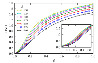
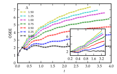
The method proposed here can be used to simulate the real time evolution of a wide range of models at finite temperature, for local operators such as the spin projection at a given site, a local current, or correlations of local operators (e.g. Green’s functions). We start by analyzing the complexity of both constituents of the method, the evolution of the density matrices and the time evolution of operators in the Heisenberg picture. We quantify the complexity in terms of the OSEE [19] which is an operator space analogue of the entanglement entropy for quantum states, defined as $S^{\sharp}(x)=-{\rm tr}[\hat{R}\log_{2}\hat{R}]$ for $\hat{R}={\rm tr}_{E}({\left|x\right)}{\left(x\right|})$. The bipartition is chosen symmetrically and thus the environment $E$ in the partial trace includes half of the system. The effective bond dimension then scales as $\exp(S^{\sharp}(x))$ with the OSEE. For density matrices, it was also observed [17] that the OSEE is related to the quantum mutual information which quantifies the total correlations between two parts of the system.

Figure 1: Operator space entanglement entropy (OSEE) in the evolution of density matrices $\rho(\beta)$ in the inverse temperature $\beta$ (left) and the local current operator $j_{n/2}(t)$ (right) for the XXZ model on $100$ sites with $\Delta$ indicated in the legends. Bond dimensions are $D=1024$ and $D=1200$, respectively. A logarithmic dependence in (imaginary) time is observed in both cases (see the insets in a semi-log scale).

We first consider a spin-$1/2$ XXZ model with open boundary conditions described by the Hamiltonian

$$H=\sum_{l=1}^{n-1}\Big{(}\sigma_{l}^{x}\sigma_{l+1}^{x}+\sigma_{l}^{y}\sigma_{l+1}^{y}+\Delta\sigma_{l}^{z}\sigma_{l+1}^{z}\Big{)},$$ (4)

where $\Delta$ is the anisotropy parameter. The OSEE of the initial state $\rho(\beta=0)$ is zero (the fully mixed state is separable). As shown in Fig. 1 (left), we observe logarithmic growth of the OSEE in the inverse temperature [17]. Furthermore, we simulate the Heisenberg evolution (3) of the spin current flowing between sites $m$ and $m+1$, $j_{m}=i(\sigma_{m}^{+}\sigma_{m+1}^{-}-\sigma_{m}^{-}\sigma_{m+1}^{+})$, with $\sigma_{m}^{\pm}=(\sigma_{m}^{x}\pm i\sigma_{m}^{y})/2$ for $m=n/2$. The results in Fig. 1 (right) show the logarithmic growth of OSEE which is an extension of the results in [14]. Similar to the evolution of density matrices, we observe an increase of OSEE for larger anisotropies $\Delta$ where the simulation is more expensive. The logarithmic growth of OSEE corresponds to polynomial growth of the bond dimension [14, 19] and the simulation can be performed efficiently. We note that the computational cost is expected to grow exponentially [14] for non-integrable systems, like in other similar methods.

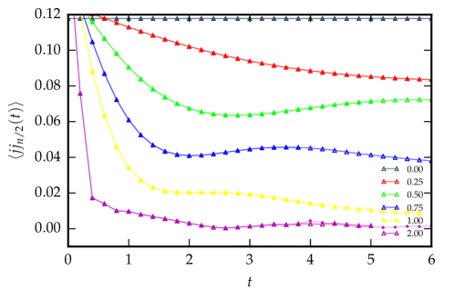
The simulation of the density matrices and the local operators can now be used to calculate e.g. the spin current correlation function $\langle jj_{n/2}(t)\rangle_{\beta}$. The results are shown in Fig. 2, with an inverse temperature $\beta=0.25$. The infinite-time limit of these current-correlations yields the Drude weight which can be used to signal ballistic transport in various integrable models, see [22]. For the XXZ chain similar results were obtained in Refs. [23, 13, 24], a detailed discussion is however beyond the scope of this manuscript and will be presented elsewhere. When compared to Ref. [13] (with our time scale multiplied by a factor of 4 due to the spin operators) we observe, on one hand, that the reachable times are approximately twice as large in the gapped regime ($\Delta=2$ in Fig. 2) with a maximal bond dimension $D=1000$. On the other hand, the computation in the gapless regime, $\Delta<1$, is less demanding and the curves obtained with a smaller bond dimension $D=800$ are essentially indistinguishable in Fig. 2. This is in complete agreement with the picture obtained from the OSEE scaling. In turn, for small $\Delta$ the simulation can be pushed beyond the time scale shown in Fig. 2, similarly to Ref. [13].

Figure 2: Current correlation function for the XXZ model on $100$ sites for various $\Delta$ and fixed $\beta=0.25$. Different symbols correspond to bond dimensions $D=800$ (circles) and $D=1000$ (triangles) for the real time evolution. The error in $\rho(\beta)$ is negligible for $D=200$.

As another illustration of the method we calculate the Green’s functions of the single impurity Anderson model which can be mapped [25, 26] to an XXZ-like model

$$H=\sum_{j=-\infty}^{\infty}\tau_{j}(\sigma_{j}^{+}\sigma_{j+1}^{-}+\sigma_{j}^{-}\sigma_{j+1}^{+})+Un_{0}n_{1}+\epsilon_{f}(n_{0}+n_{1})$$ (5)

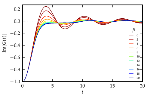
with $n_{j}=\sigma_{j}^{-}\sigma_{j}^{+}$ and the interaction strength $U$. The hopping parameters $\tau_{-1}=\tau_{1}$ are given by the hybridization whereas the rest of $\tau_{j}$ are determined from the discretization of the bath (and $\tau_{0}=0$), see [26] for details. The interaction term is only present between sites $0$ and $1$ (corresponding to spin-$\uparrow$ and spin-$\downarrow$ of the impurity) which allows longer acessible times and lower temperatures. We simulate the single particle Green’s function $G(t)=-i\langle\{f_{\uparrow}^{\dagger},f_{\uparrow}(t)\}\rangle_{\beta}$ where $f_{\uparrow}$ is the annihilation operator at the impurity for spin-$\uparrow$, written as $f_{\uparrow}=(\prod_{j<0}\sigma_{j}^{z})\sigma_{0}^{+}$ due to Jordan-Wigner transformation. Despite the nonlocality, the Heisenberg evolution of this operator can be simulated efficiently [14, 19]. We actually simulate Majorana operators $w=f_{\uparrow}+f_{\uparrow}^{\dagger}$ and $w^{\prime}=i(f_{\uparrow}-f_{\uparrow}^{\dagger})$ which are hermitian and allow the simulation in the real arithmetics. The results for the imaginary part of the Green’s function, shown in Fig. 3, can be used to calculate the spectral functions (see e.g. Ref.[27, 28, 29]) by means of a Fourier transform which will be in detail presented elsewhere.

Figure 3: Temporal Green’s function for the single impurity Anderson model (5) for $U=1$, $\tau_{j}=\frac{1}{2}$, $\tau_{0}=0$, and the particle-hole symmetric $\epsilon_{f}=-U/2$ where local Coulomb correlations are most pronounced.

4 Conclusions

We have proposed a tensor network method to simulate the real time dynamics of one dimensional quantum many-body systems at finite temperatures. The main advantage of the method is that it decouples the real time evolution from the imaginary evolution in the inverse temperature such that two independent simulations give the results for all combinations temperature–time. Furthermore, the simulations are done in real arithmetics. The method is most useful for integrable systems where the costs grow polynomially, and systems close to the integrability where the asymptotic exponential growth only appears at later times. The method can also be used to study nonequilibrium impurity physics [30], in particular current-voltage characteristics of strongly correlated nanostructures in the non-linear response regime. The proposed framework can be extended to two dimensional systems described in terms of projected entangled pair states [31] (see B); albeit with significantly higher computational costs.

Appendix A Algorithm

In Table 1 we present a algorithm to simulate the real time evolution at finite temperatures. In particular, we explain how to generate the super operators $\hat{\chi}$ and $\hat{H}$ for a one-dimensional system of $n$ sites with a local dimension $d$ and a Hamiltonian operator $H$. Let us first decompose the Hamiltonian into a sum of local product operators

$$H=\sum_{\mu}H_{1}^{(\mu)}+\sum_{\nu}H_{2}^{(\nu)},$$ (6)

where $H_{1}^{(\mu)}$ are local operators of dimension $d\times d$ and $H_{2}^{(\nu)}$ are two-site operators of dimension $(d\times d)\times(d\times d)$. The local Hilbert space for one site is generated by a set of $d^{2}$ Gell-Mann matrices $\{\sigma^{j},\,j=0,1,\ldots,d^{2}-1\}$ of dimension $d\times d$ where $\sigma^{0}=\mathbf{1}$ is the identity. The super operators $\hat{\chi}$ and $\hat{H}$ are defined as $\hat{\chi}:a\mapsto Ha$ and $\hat{H}:a\mapsto[a,H]$.

Practical algorithm for the calculation of $\langle ba(t)\rangle_{\beta}$

1. Assume a one-dimensional system of $n$ sites with a local dimension $d$ and Hamiltonian $H$ of the form (6)

2. Set up Gell-Mann matrices $\{\sigma^{j},\,j=0,1,\ldots,d^{2}-1\}$

3. Construct super-maps $\hat{\chi}$ and $\hat{H}$

4. Construct a MPS representation of the the unit ${\left|e\right)}$

5. Construct a MPS representation for the initial operator ${\left|a\right)}$

6. Simulate ${\left|\rho(\beta)\right)}={\rm e}^{-\beta\hat{\chi}}{\left|e\right)}$ using tDMRG and save ${\left|\rho(\beta)\right)}$ for various inverse temperatures $\beta$

7. Simulate ${\left|a(t)\right)}={\rm e}^{-it\hat{H}}{\left|a\right)}$ using tDMRG and save ${\left|a(t)\right)}$ for various times $t$

8. Construct $\hat{b}$ from $b$ such that $\hat{b}:x\mapsto bx$ (in the same way as $\hat{\chi}$ from $H$).

9. For all $t$ and $\beta$, calculate ${\left(\rho(\beta)\right|}\hat{b}{\left|a(t)\right)}$ and ${\left(\rho(\beta)|e\right)}$.

Table 1: Practical algorithm to simulate a time correlation function $\langle ba(t)\rangle_{\beta}$ at an inverse temperature $\beta$.

The thermal super-map $\hat{\chi}$ thus contains the same number of product operators as the hamiltonian

$$\hat{\chi}=\sum_{\mu}\hat{\chi}_{1}^{(\mu)}+\sum_{\nu}\hat{\chi}_{2}^{(\nu)},$$

where single-site terms are transformed to $d^{2}\times d^{2}$ matrices

$$[\hat{\chi}_{1}^{(\mu)}]_{j,l}=d^{-1}{\rm tr}\big{[}(\sigma^{j})^{\dagger}H_{1}^{(\mu)}\sigma^{l}\big{]},\qquad j,l=0,1,\ldots,d^{2}-1$$

and the two-site terms to $d^{2}\times d^{2}\times d^{2}\times d^{2}$ tensors

$$[\hat{\chi}_{2}^{(\nu)}]_{j_{1},j_{2},l_{1},l_{2}}=d^{-2}{\rm tr}\big{[}(\sigma^{j_{1}}\otimes\sigma^{j_{2}})^{\dagger}H_{2}^{(\nu)}(\sigma^{l_{1}}\otimes\sigma^{l_{2}})\big{]}.$$

The super-map $\hat{H}$ contains twice as many local terms as the Hamiltonian operator (due to the commutator), namely

$$\hat{H}=\sum_{\mu}(\hat{H}_{1}^{(2\mu-1)}+\hat{H}_{1}^{(2\mu)})+\sum_{\nu}(\hat{H}_{2}^{(2\nu-1)}+\hat{H}_{2}^{(2\nu)}).$$

The single-site terms are obtained as

$$[\hat{H}_{1}^{(2\mu-1)}]_{j,l}=d^{-1}{\rm tr}\big{[}(\sigma^{j})^{\dagger}\sigma^{l}H^{(\mu)}\big{]}$$

and

$$[\hat{H}_{1}^{(2\mu)}]_{j,l}=d^{-1}{\rm tr}\big{[}(\sigma^{j})^{\dagger}H^{(\mu)}\sigma^{l}\big{]}.$$

and similarly for the two-site terms.

Note that we can and we should (to work in real arithmetics) use a different basis set $\{\sigma_{\nu}\}$ for $\hat{\chi}$ and $\hat{H}$,real matrices for the former and Hermitian for the latter.

The transformation from the Hamiltonian to $\hat{\chi}$ and $\hat{H}$ can thus be treated as a black-box routine, providing the “Hamiltonian operators” which can be used in an imaginary (thermal) and a real (Heisenberg picture) time evolution – using an existing implementation of the time dependent DMRG algorithm (tDMRG) [5].

Appendix B Two-dimensional systems with PEPS

Here we briefly sketch the way how the method can be extended to two dimensional systems. In principle, the method can already be used for small two-dimensional systems as-is, represented by a matrix product state in a snake-like structure [1, 5] which gives remarkably accurate results for the ground states, see e.g. Ref. [32] for a recent study. However, for more extended two-dimensional systems the preferred description is given in terms of Projected Entangled Pair States (PEPS) [31]. Here we show how our method can be used with PEPS. For simplicity we assume a spin-$1/2$ quantum system on a $m\times n$ rectangular lattice. Any operator can be written as a superposition of basis operators

$$a=\sum_{\nu_{i,j}}a_{\underline{\nu}}\,\sigma_{1,1}^{\nu_{1,1}}\cdots\sigma_{1,n}^{\nu_{1,n}}\cdots\sigma_{m,n}^{\nu_{m,n}}$$

for $\nu_{i,j}\in\{0,x,y,z\}$ and the corresponding elements of the operator space ${\left|a\right)}$ can be represented by a PEPS-Ansatz,

$${\left|a\right)}=\sum_{\nu_{1,1}\cdots\nu_{m,n}}{\rm tr}\big{[}\mathbf{A}^{[1,1]\nu_{1,1}}\cdots\mathbf{A}^{[m,n]\nu_{m,n}}\big{]}{\left|\nu_{1,1},\ldots,\nu_{m,n}\right)}.$$ (7)

The trace in (7) must be understood as a tensor-trace, for details on PEPS see Ref. [31]. The operator $a$ is now represented in terms of rank-$4$ tensors $\mathbf{A}^{[i,j]\nu_{i,j}}\in\mathbb{R}^{D_{\rm l}\times D_{\rm u}\times D_{\rm d}\times D_{\rm r}}$ where $(D_{\rm l},D_{\rm u},D_{\rm d},D_{\rm r})$, are the dimensions of the bonds connecting the site $[i,j]$ to the neighboring sites (left,up,down,right), respectively.

The method proposed in the main text can now be used exactly in the same way as in the one-dimensional case, by operating on PEPS instead of MPS. The super-maps $\hat{\chi}$ and $\hat{H}$ are identical to the one-dimensional case and generate the evolution in the Heisenberg picture

$${\left|a(t)\right)}={\rm e}^{-it\hat{H}}{\left|a\right)}$$

and the thermal evolution of the density matrix

$${\left|\rho(\beta)\right)}={\rm e}^{-\beta\hat{\chi}}{\left|e\right)}.$$

The only difference to the one-dimensional case is that the computation with PEPS is significantly more expensive and an accurate description might require a considerably increased computational effort. In particular, the complexity of the real time evolution scales as $O(D^{12})$ (as opposed to $O(D^{3})$ for matrix product states). It is not clear at present whether the computational costs still scale polynomially in time like in the one-dimensional case, however, results from the ground state simulations are consistent with this conjecture.

References

- [1] S. R White, Phys. Rev. Lett. 69, 2863 (1992).
- [2] S. Östlund and S. Rommer, Phys. Rev. Lett. 75, 3537 (1995).
- [3] G. Vidal, Phys. Rev. Lett. 91, 147902 (2003); Phys. Rev. Lett. 93, 040502 (2004).
- [4] F. Verstraete, J. J. García-Ripoll, and J. I. Cirac, Phys. Rev. Lett. 93, 207204 (2004).
- [5] U. Schollwöck, Rev. Mod. Phys. 77, 259 (2005).
- [6] U. Schollwöck, Ann. Phys. 326, 96 (2011).
- [7] S. R. White and A. E. Feiguin, Phys. Rev. Lett. 93, 076401 (2004).
- [8] A. J. Daley, C. Kollath, U. Schollwöck, and G. Vidal, J. Stat. Mech. (2004) P04005
- [9] A. E. Feiguin and S. R. White, Phys. Rev. B 72, 220401(R) (2005).
- [10] M. Zwolak and G. Vidal, Phys. Rev. Lett. 93, 207205 (2004).
- [11] T. Barthel, U. Schollwöck, and S. R. White, Phys. Rev. B 79, 245101 (2009).
- [12] A. E. Feiguin and G. A. Fiete, Phys. Rev. Lett. 106, 146401 (2011).
- [13] C. Karrasch, J. H. Bardarson, and J. E. Moore, Phys. Rev. Lett. 108, 227206 (2012); New J. Phys. 15, 083031 (2013)
- [14] T. Prosen and M. Žnidarič, Phys. Rev. E 75, 015202(R) (2007).
- [15] M. J. Hartmann, J. Prior, S. R. Clark and M. B. Plenio, Phys. Rev. Lett. 102, 057202 (2009).
- [16] T. Barthel, U. Schollwöck, and S. Sachdev, arXiv:1212.3570; T. Barthel, New J. Phys. 15, 073010 (2013).
- [17] M. Žnidarič, T. Prosen, and I. Pižorn, Phys. Rev. A 78, 022103 (2008).
- [18] T. Prosen and M. Žnidarič, J. Stat. Mech. (2009) P02035.
- [19] T. Prosen and I. Pižorn, Phys. Rev. A 76, 032316 (2007); I. Pižorn and T. Prosen, Phys. Rev. B 79, 184416 (2009).
- [20] V. Eisler and I. Peschel, J. Stat. Mech. (2007) P06005.
- [21] P. Calabrese and J. Cardy, J. Stat. Mech. (2007) P10004.
- [22] F. Heidrich-Meisner, A. Honecker and W. Brenig, Eur. Phys. J. Spec. Top. 151, 135 (2007)
- [23] J. Sirker, R. G. Pereira, and I. Affleck, Phys. Rev. Lett. 103, 216602 (2009); Phys. Rev. B 83, 035115 (2011).
- [24] C. Karrasch, J. Hauschild, S. Langer, and F. Heidrich-Meisner, Phys. Rev. B 87, 245128 (2013).
- [25] R. Bulla, T. A. Costi, and T. Pruschke, Rev. Mod. Phys. 80, 395 (2008).
- [26] A. Weichselbaum, F. Verstraete, U. Schollwöck, J. I. Cirac and J. von Delft, Phys. Rev. B. 80, 165117 (2009).
- [27] A. Weichselbaum and J. von Delft, Phys. Rev. Lett. 99, 076402 (2007).
- [28] R. Peters, T. Pruschke, and F. B. Anders, Phys. Rev. B 74, 245114 (2006).
- [29] A. Isidori, D. Roosen, L. Bartosch, W. Hofstetter, and P. Kopietz, Phys. Rev. B 81, 235120 (2010).
- [30] F. Heidrich-Meisner, A. E. Feiguin, and E. Dagotto, Phys. Rev. B 79, 235336 (2009); J. Eckel, F. Heidrich-Meisner, S.G. Jakobs, M. Thorwart, M. Pletyukhov, and R. Egger New J. Phys. 12, 043042 (2010).
- [31] F. Verstraete and J. I. Cirac, arXiv:cond-mat/0407066.
- [32] S. Depenbrock, I. P. McCulloch, and U. Schollwöck, Phys. Rev. Lett. 109, 067201 (2012).