Ellipticity and prolaticity of the initial gravitational-shear field at the position of density maxima
Abstract
Dark-matter haloes are supposed to form at the positions of maxima in the initial matter density field. The gravitational-shear field’s ellipticity and prolaticity that serve as input for the ellipsoidal-collapse model, however, are derived from a distribution that does not take the additional maximum constraint into account. In this article, I quantify the variations of the most probable and the expected values of the ellipticity and the prolaticity when considering this additional constraint as well as the implications for the ellipsoidal-collapse model. Based on the statistics of Gaussian random fields, it is possible to set up a joint distribution for the eigenvalues of the gravitational-shear tensor and the matter density that incorporates the maximum constraint by invoking a vanishing first derivative and a negative definite second derivative of the density field into the calculation. In the density range relevant for cosmological structure formation, both the most probable and the expected value of the ellipticity calculated from the standard distribution used in the literature are about 3–8 per cent higher compared to the ones calculated under the additional assumption of a density maximum. Additionally, the analogous quantities for the prolaticity do not vanish but acquire slightly positive values in the range of –. For large overdensities, the predictions from both distributions converge. The values for and derived from the ellipsoidal-collapse model using the standard distribution for the initial ellipticity and prolaticity are up to 4 and 6 per cent higher, respectively, than those obtained taking the additional maximum constraint into account in the range of – in mass and 0–2 in redshift.
keywords:
cosmology: theory – methods: analytical – dark matter – cosmological parameters – galaxies: clusters: general1 Introduction
Galaxies and galaxy clusters as collapsed objects are supposed to form from peaks in the initial matter density field. After an overdense patch has decoupled from the Hubble expansion, the extent of this patch is supposed to reach a maximum value, then to shrink again until the collapse stops when the structure reaches virial equilibrium. Analytical models for this evolution include the spherical-collapse model (e.g. Gunn & Gott 1972; Lahav et al. 1991; Lacey & Cole 1993; Wang & Steinhardt 1998; Pace, Waizmann & Bartelmann 2010) and the ellipsoidal-collapse model (e.g. Icke 1973; White & Silk 1979; Barrow & Silk 1981; Bartelmann, Ehlers & Schneider 1993; Eisenstein & Loeb 1995; Bond & Myers 1996).
Most of the theories of inflation predict that the density field is initially a random field whose non-Gaussianity is small (Planck Collaboration XXIV, 2013). Since also derivatives and integrals of Gaussian random fields are again Gaussian, a multivariate Gaussian random field can be used to derive the initial number density of peaks in the density field as a function of peak height by applying respective constraints to the density field’s first and second derivatives (Bardeen et al., 1986).
Not only can the density field be described as a Gaussian random field, but through Poisson’s equation, also the gravitational field has to follow a Gaussian distribution and therefore also the eigenvalues of the gravitational-shear tensor can be derived from the statistics of Gaussian random fields (Doroshkevich, 1970; Zel’dovich, 1970). These eigenvalues can be combined to define the ellipticity and the prolaticity of the gravitational-shear field whose distribution for a given value of the overdensity can be derived by transformation of variables (Bardeen et al. 1986; van de Weygaert & Bertschinger 1996; Sheth, Mo & Tormen 2001) and either their most probable or their expected values are used to set the initial conditions in the ellipsoidal-collapse model by Bond & Myers (1996).
However, this distribution does not take into account that haloes should form at maxima in the density field, but rather yields the probability density for ellipticity and prolaticity for any overdensity irrespective if it is taken at a maximum or not. Recently, attempts have been made to take the maximum constraint into account when calculating the gravitational-shear tensor’s conditional eigenvalues for given eigenvalues of the density’s Hessian (Rossi, 2012) as well as the conditional ellipticity and prolaticity from them (Rossi, 2013) by extending the formalism of Doroshkevich (1970) and Sheth et al. (2001). Rossi (2012, 2013), however, only covers one of the two constraints necessary for a density maximum, i.e. that the density’s Hessian has to be negative definite. The other necessary condition, namely the vanishing first derivative of the density, is not taken into account. Additionally, Rossi (2013) does not derive the distribution for the unconstrained ellipticity and prolaticity necessary for the ellipsoidal-collapse model by Bond & Myers (1996).
Comparisons to numerical simulations, however, reveal that the simple picture of this model is not fully realized. For example, Ludlow & Porciani (2011) found out that not all collapsed haloes form from a density peak in the initial Gaussian random field whose characteristic mass is close to that of the halo. Only 70 per cent of well-resolved haloes in their simulation possess this preference, whereby heavier haloes have the tendency to stay near the position of the initial peak, while low-mass haloes increasingly tend to move away from the location of the initial density peak due to the gravitational influence of the surrounding structure. Also Elia, Ludlow & Porciani (2012) claim that relating virialized haloes to density peaks of a given height is too simplistic to forecast the density bias parameters correctly with the analytic model by Desjacques & Sheth (2010).
The works by both Ludlow, Borzyszkowski & Porciani (2011) and Despali, Tormen & Sheth (2013) have shown that the initial protohaloes are not spherical as assumed in the model by Bond & Myers (1996) but have already a rather ellipsoidal shape. Additionally, they found out that for most haloes the deformation and the mass tensors are all well aligned and that the longest axis corresponds to the direction of maximal compression. While the first result corresponds to one of the main assumptions of the ellipsoidal-collapse model, the latter is in direct contrast with it. Accounting for these deviations in the analytical model results in lowering the critical overdensity significantly for a given mass (Ludlow et al., 2011) and in a possible inversion of axes so that the initially shortest axis might become the longest during the evolution and vice versa (Ludlow et al., 2011; Despali et al., 2013).
Despite the differences between results from numerical simulations and the simple ellipsoidal-collapse model by Bond & Myers (1996), we will focus on the latter taking only into account modifications by Angrick & Bartelmann (2010) in the following to clarify if incorporating the maximum constraint alters the results from this model for the critical overdensity and the virial overdensity more significantly than the other aforementioned effects found in numerical simulations.
In this article, I will show how the distribution of the gravitational shear’s ellipticity and prolaticity at the position of density maxima can be derived from the statistics of Gaussian random fields by accounting for the two aforementioned necessary constraints (vanishing first derivative and negative definite Hessian). In Section 2, I give a short introduction to Gaussian random fields and show step-by-step how the targeted distribution can be calculated invoking the technique to derive number densities from multivariate Gaussians of the relevant quantities based on Bardeen et al. (1986) and how the constraint for the density’s Hessian can be properly considered without diagonalisation. In Section 3, I compare the results from three distributions to each other. The first one incorporates only the constraint for the density’s Hessian to be negative definite, the second one includes additionally the constraint for the vanishing first derivative of the density, and the third one is the distribution of Sheth et al. (2001) that does not take any of these constraints into account. Furthermore, I present the implications for the ellipsoidal-collapse model by Bond & Myers (1996), especially on the linear overdensity and the virial overdensity in this section. Finally, I summarize the main results of this article in Section 4.
2 The conditional distribution for ellipticity and prolaticity
In this section, I derive the conditional probability for the ellipticity and the prolaticity of the gravitational shear from the statistics of Gaussian random fields. First, I give a brief overview over the theoretical background of Gaussian random fields based on Bardeen et al. (1986, see also Angrick & Bartelmann 2009 for further information). Hence, I also adopt for the random field and and for its first and second derivatives, respectively.
2.1 Theoretical background
An -dimensional random field assigns a set of random numbers to each point in -dimensional space. A joint probability function can be declared for arbitrary points with as the probability that the field , considered at the points , has values between and .
A Gaussian random field is a field whose joint probability functions are multivariate Gaussians. Let with be a set of Gaussian random variables with means and . The covariance matrix M has the elements , and the joint probability function of the Gaussian random variables is
| (1) |
with the quadratic form
| (2) |
These random variables can, for example, not only include the field , but also its derivatives, integrals or linear combinations thereof since they are also Gaussian.
In the following, I will focus on the density contrast defined by that is defined on the three-dimensional Euclidean space with coordinates . Here, is the position-dependent density and is the cosmic background density. Hence, I will set from now on.
This homogeneous Gaussian random field with zero mean is fully characterized by its two-point correlation function or equivalently its Fourier transform, the power spectrum . Its spectral moments are defined by
| (3) |
where is the Fourier transform of the filter function , and is its filter size. In the following, I adopt Gaussian filtering, hence
| (4) |
The zeroth-order spectral moment is the power spectrum’s variance.
It is possible to scale the field as well as its derivatives with corresponding spectral moments so that they become dimensionless. I will denote these reduced fields with a tilde, e.g. , , and , where now and . A quantity that will be used more often in the next sections is a special combination of the first three spectral moments, .
The elements of the gravitational-shear tensor (Zel’dovich, 1970) contain the scaled second derivatives of the gravitational potential ,
| (5) |
where is Newton’s constant, so that by Poisson’s equation. I will denote the eigenvalues of with , where . The ellipticity and the prolaticity are combinations of these eigenvalues,
| (6) |
Ordering the eigenvalues in the way , as it is commonly done in the literature, imposes the constraints and for . Since a spherical configuration has , this is equivalent to . While the ellipticity measures the anisotropy in the --plane, the prolaticity quantifies the shape perpendicular to it: if , the configuration is prolate, for it is oblate. Note that ellipticity and prolaticity are defined on the linear density field and should not be confused with the shape of the final halo.
Following Bardeen et al. (1986), the conditional probability for the random variables and given a maximum of reduced height can be expressed as
| (7) |
where, as already mentioned above, is the reduced first derivative of and is the corresponding reduced Hessian, which has only six independent components since it is symmetric. Note that only those subvolumes contribute to the integral for which is negative definite, i.e. its three eigenvalues are negative. This is taken into account by the function which has the property
| (8) |
I will discuss in Section 2.3 how the function can be specified explicitly.
2.2 The joint probability of relevant quantities
To calculate , I shall start with establishing the 15-dimensional joint probability of reduced variables to evaluate the numerator of equation (7).
The correlation matrix M incorporates all auto- and cross-correlations of the various random variables. These are
| (9) | ||||||
| (10) |
where is the Kronecker symbol and the quantity is a combination of Kronecker symbols given by . All other correlations apart from those listed above vanish (cf. also Bardeen et al., 1986; Rossi, 2012). Defining the vector of random variables
| (11) |
the correlation matrix M looks like
| (12) |
where the different submatrices are given by
| (13) |
The determinant of M is
| (14) |
and the inverse of M is
| (15) |
where 1 and are defined as above and
| (16) |
Rotating the coordinate system such that becomes diagonal and assuming that its eigenvalues are ordered like , Bardeen et al. (1986) showed that the volume element can be written as
| (17) |
Note that the two matrices and do not commute and hence cannot be diagonalized simultaneously.
Therefore, the off-diagonal elements of do not vanish, whereas , and the diagonal of is populated by its eigenvalues after the rotation.
The circumstance that and do not commute can be shown as follows. The elements of the density’s Hessian are given by
| (18) |
where is chosen as an abbreviation for the scaled fourth derivative of the gravitational potential analogous to equation (5). The commutator of the two matrices and is defined as . Written in components, it is given by
| (19) |
where I have used that and . Hence, the two matrices and do not commute.
Switching from the eigenvalues to the new variables , and (cf. equation 6), the Jacobi determinant of the transformation introduces an additional factor so that
| (20) |
Starting from equations (1) and (2) with the random variables (11), inverse (15) of the correlation matrix and the correlation matrix’ determinant (14), one can construct the multivariate Gaussian probability distribution (1). Then, I rotate the coordinate system such that the matrix becomes diagonal and switch from the three eigenvalues to the new variables , , and , taking into account that the differentials transform like shown in equations (17) and (20). Finally, since I concentrate on maxima, I set so that
| (21) |
In that way, the integrand in the numerator of equation (7) can be written as
| (22) |
where I have introduced the abbreviations
| (23) |
and with
| (24) |
2.3 Sylvester’s criterion
To evaluate the numerator of equation (7), I have to integrate over those parts of the volume spanned by the matrix elements of for which the latter is negative definite. This can be achieved by taking into account the following criterion. A Hermitian matrix is positive definite if and only if all its leading principal minors are positive, where the th leading principal minor is the determinant of its upper left submatrix. This is known as Sylvester’s criterion. Since the negative of a positive definite and Hermitian matrix is negative definite, this implies that all odd principal minors have to be negative and all even principal minors have to be positive.
Thus, the function introduced in equation (7) can be specified as
| (25) |
When integrating equation (22) numerically over the various matrix elements, I also multiply it by the function and integrate over all six independent elements from to .
2.4 The number density of maxima in the density field
In analogy to the way I have derived equation (22), it is possible to derive the joint probability . Apart from the correlations and , which are already given in equation (9), the auto-correlation of the density contrast, and the cross-correlation are the only non-vanishing contributions that are needed for the derivation. The vector of random variables that enters equation (1) in this case has 10 components and can be written by
| (26) |
so that the correlation matrix looks like
| (27) |
where , 1, and A are defined in equation (13), whereas and are vectors of the form
| (28) |
respectively. Inverting M leads to
| (29) |
where
| (30) |
At this point, it is most efficient to rotate the coordinate system into the eigensystem of . Note that this rotation is different from the one applied when calculating equation (22), since there I aimed at diagonalising instead of to introduce the ellipticity and the prolaticity , which are defined in the eigensystem of . The calculation in this section, however, corresponds to deriving the number density of maxima of a certain height (see below), which is a quantity independent of the choice of the coordinate system’s rotation so that I am free to choose a different rotation from the one applied to derive equation (22).
Using the ordered eigenvalues of the density’s reduced Hessian , the volume element can be written after the diagonalisation analogously to equation (17) as
| (31) |
Switching to the new variables , and , introduced in equation (23), which are functions of the eigenvalues after the rotation,
| (32) |
introduces an additional factor through the Jacobian of the transformation,
| (33) |
The last step again is to set so that
| (34) |
where I have used that is negative if is negative definite.
Applying all the various steps mentioned above, the integrand in the denominator of equation (7) can be written as
| (35) |
To evaluate the denominator of equation (7), I have to integrate over the eigenvalues from to 0, or, since I have transformed to the new variables , , and , integrate over them in the proper range. The condition translated to the new variables reads
| (36) |
Note that the variables and are negative in contrast to the analogous variables and for the gravitational-shear tensor.
It turns out that the integrations over and can be done analytically, while the integration over has to be done numerically. The denominator of equation (7) is equal to the number density of maxima of the reduced density field if multiplied by a factor . The latter can be written as
| (37) |
with
| (38) |
Now all the ingredients to express the probability to find the ellipticity and the prolaticity of the gravitational-shear field in the range and given a density peak of height are at hand. To summarize, after scaling it to the reduced density , the probability is given by the ratio (7), where the numerator is expressed by equation (22) together with equations (23) and (24), and the denominator by equations (37) and (38) except the factor . The function defined in equation (25) offers a nice way to take into account the constraint that equation (22) has to be integrated only over those subvolumes for which the matrix is negative definite.
2.5 Comparison to the ansatz of Rossi
Rossi (2012) derives a conditional probability for the reduced shear tensor given a positive definite Hessian (see his equations 18 and 19). In the language of this paper, his probability looks like
| (39) |
where , and accounts for integration over the subvolume for which is positive definite and can thus be similarly declared as in equation (25) with the difference that all submatrices need to have positive determinants. Both and can be written as an expression analogous to the distribution of the gravitational-shear tensor’s eigenvalues derived by Doroshkevich (1970).
However, it is not possible to diagonalize both matrices and simultaneously since the commutator of the two does not vanish. Hence, the aim of Rossi (2013) is that this ansatz can be used to determine the probability from equation (39), implying that the eigenvalues of both the former matrices can be used. This, however, is not possible since only one of them can be diagonalized at once, it is not obvious how the six-dimensional integration over all entries of the matrix can be circumvented.
Furthermore, equation (39) seems incomplete in the sense that it neglects the constraint that the first derivative has to vanish for a maximum. Rossi (2012, 2013) only takes into account the Hessian which has to be positive definite,111Actually, it should be negative definite for a maximum. However, a homogeneous Gaussian random field with zero mean is symmetric in the sense that integration over subvolumes which are either positive or negative definite yields the same result. and therefore, his probability is not only based on maxima in the density field but also on areas for which the first derivative is non-zero. Equation (7) is more specific in that respect since it takes the constraint explicitly into account (see also Bardeen et al., 1986).
To quantify the difference between accounting for this additional constraint or not, I will also evaluate the conditional probability that only incorporates the constraint on the density’s Hessian. In this case, equation (7) simplifies to
| (40) |
where I integrate over the subvolumes for which is negative definite for consistency. Note the absence of the factor in both integrals in equation (40) in comparison to equation (7) which originated from the property that in the infinitesimal volume around a maximum and therefore .
Since can be derived analogously to except that the first derivative is missing since no constraints are applied to it, I will only present the final result. The integrand in the numerator of equation (40) is given by
| (41) |
while the integrand in the denominator can be written as
| (42) |
Equations (41) and (42) deviate from equations (22) and (35) only in two ways. (a) The normalizations differ because the vanishing first derivative was not taken into account in equations (41) and (42). This difference, however, drops out when taking their ratio. (b) The factor is not present in both equations. In contrast to the previous point, this additional factor does not vanish when taking the ratio since in both the numerator and the denominator, an integration over the reduced Hessian still has to be carried out.
3 Results
In this section, I present some numerical results based on the theoretical work developed in the previous section. For the calculation, I adopt a flat reference CDM model inspired by the Planck results (Planck Collaboration XVI, 2013) with matter density , dark-energy density , baryon density , a Hubble constant of in units of and power spectrum normalization . Note that by this definition, does not correspond to the eighth spectral moment but to the square root of the variance filtered on a scale of 8 Mpc. All previous values are set at redshift . The primordial spectral index of the power spectrum is set to , and I adopt the transfer function of Eisenstein & Hu (1998).
3.1 The joint distribution for ellipticity and prolaticity
In the following, I compare the distributions (7) and (40) with the distribution
| (45) |
(Sheth et al., 2001), which does not take any of the two constraints on the first derivative and the Hessian into account. For a better comparison to other papers in the literature and to simplify the connection to a mass scale, I adopt the variable
| (46) |
instead of . In the former equation, is the linear overdensity of the spherical-collapse model, and is the power spectrum’s variance exponentially filtered on the scale (cf. equation 3). Hence, for a given , the corresponding reduced density contrast is simply and the radius has to be chosen such that equation (46) is fulfilled. It is then used to calculate the higher spectral moments and from equation (3) and also .
In Table 1, I list the corresponding mass for both and for some redshifts between 0 and 1 in the cosmological model introduced at the beginning of Section 3.
| 0 | |
|---|---|
| 0.2 | |
| 0.4 | |
| 0.6 | |
| 0.8 | |
| 1 | |
| 0 | |
|---|---|
| 0.2 | |
| 0.4 | |
| 0.6 | |
| 0.8 | |
| 1 | |
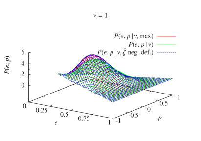
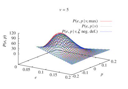
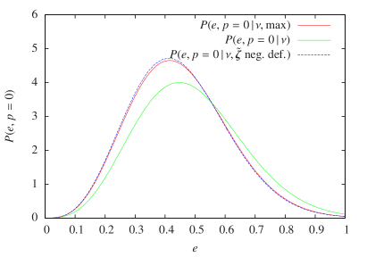
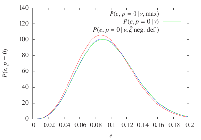
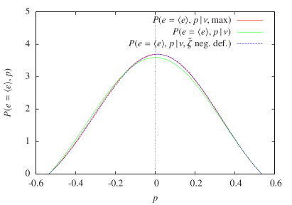
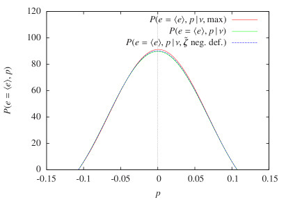
In Fig. 1, I compare the distributions (7), (40), and (45) as a function of and for two different values of . For , the distributions and (red and blue lines, respectively) coincide very well over the whole range of and , whereas peaks at a slightly larger value of and as a consequence of the normalization to unity has a smaller amplitude at the maximum compared to the two former distributions. This implies that haloes of lower mass tend to be slightly less elliptical than predicted by the standard formula (45).
For , the situation is reversed: now corresponds very well to , whereas has a larger amplitude compared to the two former distributions. The amplitude of the relative differences between the distributions, however, has shrunk, indicating that the additional constraints become the less important the higher is.
What is most important for most practical purposes, however, is not the full distribution for and , but only the values that are either expected or most probable. The expectation values of and are used e.g. by Angrick & Bartelmann (2009) to determine the initial eigenvalues for the ellipsoidal-collapse model by Bond & Myers (1996), whereas the most probable values are used by Sheth et al. (2001) to determine the ellipsoidal barrier when establishing their mass function. The expectation values of and as well as their variances can be calculated analytically for the distribution . They are as a function of given by
| (47) | ||||||
| (48) |
(Angrick & Bartelmann, 2010). The most probable values for and from the same distribution are
| (49) |
respectively (Sheth et al., 2001).
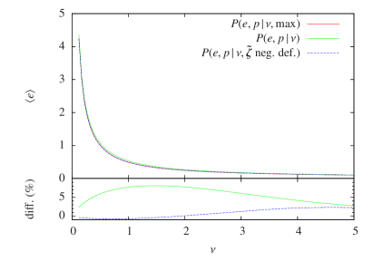
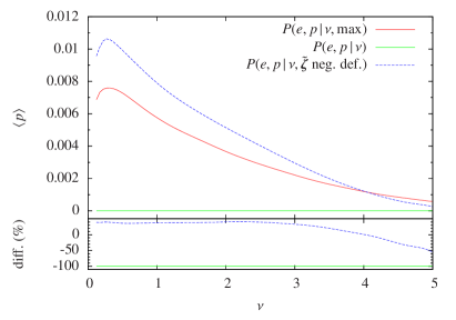
In Fig. 2, I present the expectation values for both ellipticity and prolaticity for the distributions , , and as a function of . As expected, the expectation value for the ellipticity is smaller if either both constraints for a maximum or only the constraint that the density’s Hessian has to be negative definite is taken into account. Additionally, the expected prolaticity acquires a small non-vanishing value in the latter two cases. For larger , the differences between the three distributions decrease. While the largest difference in is at with a value that is 8 per cent larger if none of the maximum constraints are taken into account, is monotonically decreasing for with increasing and has a maximal value of at for and for at the same position. Therefore, the most probable value for the prolaticity does not vanish identically for a density maximum as it is the case for arbitrary points.
Interestingly, taking the additional condition of a vanishing first derivative into account does not result in a very different (the modulus of the relative difference between the two results is 2 per cent for with a change of sign in the deviation at ), the relative difference for is practically constant with a value that is 40 per cent larger if the condition on the first derivative is neglected. It decreases until is equal for both distributions at , then changes sign and quickly reaches 50 per cent at . Although the relative change in the expected prolaticity is large if one incorporates the condition , the absolute amplitudes, however, remain rather small.
Both and at a maximum reach the values deduced from the joint probability of and not taking any of the two maximum constraints into account as for the same reason as already stated above: The higher is, the more probable it is that the maximum constraint is automatically fulfilled.
The same quantitative behaviour is found for the most probable values and . The deviations are 8 per cent for and 50 per cent for with the same dependence on as for the expectation values and so that the latter approaches zero for increasing .
In summary, the ellipticity used in analytical models of structure formation is about 3–8 per cent too high in the range of relevant for cosmology since the maximum constraint is not taken into account. The prolaticity is usually assumed to vanish, but should be slightly positive with values at the level of – in the same range.
3.2 Implications for the ellipsoidal-collapse model
In this section, I will quantify the consequences for the ellipsoidal-collapse model by Bond & Myers (1996), extended by Angrick & Bartelmann (2010), especially for the parameters and . Before, I will present the most important formulae.
The evolution of the scaled dimensionless principal axes with of a homogeneous ellipsoid, where the are the dimensional axes and is the radius of a sphere with homogeneous density that contains a mass , is governed by the following three coupled differential equations:
| (50) |
where a prime denotes differentiation with respect to the scale factor , is the universe’s expansion function, and . Here, is the density contrast inside the ellipsoid, and the are the external shear’s eigenvalues whose evolution is modelled according to the hybrid model so that
| (51) |
where is the turn-around scale factor of the th axis, is the linear growth factor of structure formation, and the are the internal-shear tensor’s eigenvalues given by
| (52) |
Note that in this type of ellipsoidal-collapse model, the ellipsoid’s principal axes are aligned with those of the external gravitational shear.
The initial conditions are chosen such that they are compatible with the Zel’dovich approximation at early times. Hence,
| (53) | ||||
| (54) |
since for which is safely fulfilled for . At this point, a change in the joint distribution for the ellipticity and the prolaticity has influence on the model’s results since the are the initial eigenvalues of the gravitational-shear tensor, whose elements were defined in equation (5). The eigenvalues are functions of , , and up to first order in and ,
| (55) | ||||
| (56) | ||||
| (57) |
implying .
The collapse of the th axis is stopped when the following virialization conditions derived from the tensor virial theorem are fulfilled,
| (58) |
The parameters and can be calculated from the ellipsoidal-collapse model by
| (59) |
where is the scale factor at which the third axis virializes.
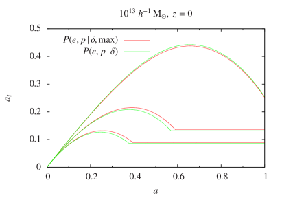
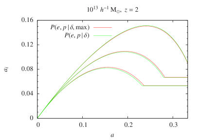
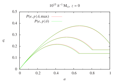
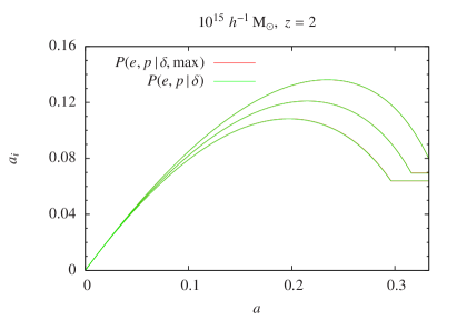
In Fig. 3, I present the evolution of the ellipsoid’s three axes as a function of the scale factor for two different virialization redshifts and two masses using either or for the determination of the axes’ initial conditions. These distributions enter the model via equations (53) and (54) since both and are dependent on the respective gravitational-shear tensor’s eigenvalue which is a linear combination of and . For clarity, I did not include the evolution of the ellipsoid’s axes for which the initial conditions are based on since the differences to the results for are negligible.
All four plots have in common that the two axes along which virialization sets in first ( and ) are smaller if the maximum constraint is not taken into account, whereas , the longest axis, is larger in comparison. Additionally, the virialization of and sets in earlier. These features are most pronounced for small masses and low redshifts.
The reason is as follows. For , is lowered, whereas is enlarged according to Fig. 2, but in terms of absolute values this effect is larger for the ellipticity than for the prolaticity. Hence, equations (55)–(57) imply that both and are lowered, whereas is enlarged so that according to equations (53) and (54), the axes and both start with slightly larger amplitudes and velocities, and is slightly smaller in both amplitude and velocity.
For large masses and high redshifts, however, the ellipsoid’s evolution differs less since a larger overdensity is needed for the ellipsoid to collapse at the redshift considered so that the change in and is much less pronounced as shown in Fig. 2. Hence, the smallest difference in the evolution can be found in Fig. 3 for the ellipsoid with virializing at . Additionally, the collapse becomes less ellipsoidal at larger masses and higher redshifts.
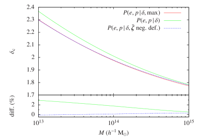
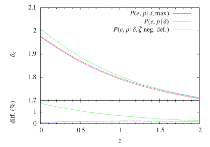
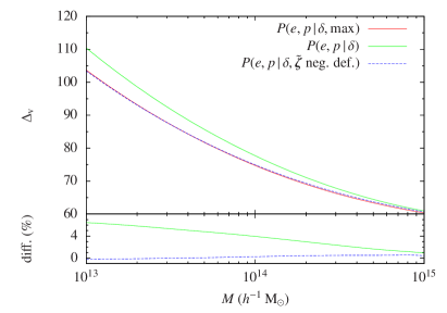
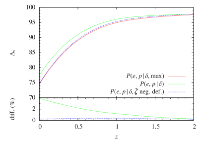
The results of this change in the axes’ evolution for the parameters and are shown in Fig. 4. The overall trend is that both parameters are lowered if additional constraints on the density’s spatial derivatives are taken into account. This effect is the stronger the lower the ellipsoid’s virialization redshift and its mass are. Additionally to the constraint that the density’s Hessian is negative definite, incorporating the second constraint of a vanishing first derivative changes both and by less than half a per cent over the whole mass and redshift ranges considered.
For ellipsoids with a mass between and and a virialization redshift between 0 and 2, is 3 per cent smaller if the maximum constraints are not accounted for, where the maximal deviation of 3 per cent is reached for and . The deviation drops to 2 per cent for and 0.5 per cent for both at .
The effect for is approximately twice as large as for with values for that are 7.5 per cent smaller if instead of is used for the initial conditions. Again, the largest deviation can be found for and . The difference drops to 4 per cent for and 1 per cent for both at .
While only the sum enters the computation of , whose evolution is then driven by the linear growth factor , the situation is different for . Here, the individual axes are initially altered due to a change of initial , and and evolve non-linearly. The at the time of virialization then determine according to equation (59). This non-linearity is the reason why the deviation for is larger than for .
4 Summary & conclusions
In the first part of this article, I have derived the probability for the gravitational-shear field’s ellipticity and prolaticity at the position of a peak in the density field with a given height. The derivation is based on the statistics of Gaussian random fields (Bardeen et al., 1986) and extends the works by Sheth et al. (2001) and Rossi (2012, 2013) as follows. In contrast to Sheth et al. (2001), I have added explicitly the maximum constraint in the calculation since it is expected that haloes form at the positions of peaks in the density field. Although Rossi (2012, 2013) started going into the same direction, they have considered the conditional eigenvalues of the matrix and the corresponding ellipticity and prolaticity. These, however, do not serve as ingredients for the ellipsoidal-collapse model by Bond & Myers (1996) since they use the ellipticity and the prolaticity derived from the eigenvalues of the matrix instead. Additionally, they considered that the density’s Hessian has to be negative definite for a maximum but did not take into account that the first derivative also has to vanish.
The main results of the first part can be summarized as follows:
-
•
The gravitational-shear tensor and the density’s Hessian cannot be diagonalized simultaneously. Since the eigenvalues of are needed for the definition of the ellipticity and prolaticity as used in the ellipsoidal-collapse model by Bond & Myers (1996), the priority is on the diagonalisation of so that first, the constraint that the density’s Hessian has to be negative definite for a maximum can only be considered via Sylvester’s criterion and second, the full six-dimensional integration over has to be carried out.
-
•
The conditional probability for and given a density maximum of height including the constraints on both the first and second derivatives is given by (7) after rescaling to . The numerator can be calculated by integrating equation (22) multiplied by the function (25) that takes into account Sylvester’s criterion for a negative definite Hessian of the density, while the denominator is given by equation (37) divided by together with equation (38).
-
•
The conditional probability for and only incorporating the constraint that the density’s Hessian has to be negative definite is given by (40) in rescaled quantities, where the numerator can be calculated using equation (41), while the denominator is given by equation (43) together with equation (44).
-
•
The distribution of and incorporating the maximum constraint peaks at lower ellipticities and slightly positive prolaticities compared to the unconstrained one by Sheth et al. (2001).
-
•
As a consequence, both the expected and the most probable ellipticities are about 3–8 per cent larger in the range if the maximum constraint is not accounted for with the largest deviation at around . Both the expected and the most probable prolaticity have slightly positive values at the level of – reaching the largest absolute value at .
-
•
Both expected and most probable values for ellipticity and prolaticity from the distribution tend to converge to the values from the distribution for since the larger , the more likely is the maximum constraint automatically fulfilled.
In the second part of this article, I quantify the impact on the ellipsoidal-collapse model by Bond & Myers (1996) that was slightly modified and extended by Angrick & Bartelmann (2010) if either both maximum constraints or only the constraint on the density’s Hessian are/is taken into account, especially on the parameters and . The main results of the second part are as follows.
-
•
If none of the additional constraints is taken into account, the resulting linear overdensity is up to 4 per cent higher compared to the constrained distribution , and the virial overdensity is up to 6 per cent higher in the mass range of – and in the redshift range of 0–2. The deviations between the results from the two distributions decrease for both increasing mass and redshift.
-
•
The results on the parameters and differ less than 0.5 per cent if the constraint that the first derivative has to vanish is neglected.
Although the calculation of and at the position of density maxima cannot be carried out analytically any more, and it is computationally rather expensive (1 min on an Intel Pentium(R) with 2.80 GHz) due to an eight-dimensional integral that has to be carried out, the final results for both and only change mildly. Therefore, it depends on the individual application of the ellipsoidal-collapse model if the gain of accuracy of a few percent in both parameters is more important than the long computation time that can be saved if the maximum constraint is neglected.
Acknowledgements
I want to thank M. Bartelmann for carefully reading the manuscript and for the suggestions that helped to improve it and B. M. Schäfer for the discussions that finally led to the implementation of Sylvester’s criterion.
References
- Angrick & Bartelmann (2009) Angrick C., Bartelmann M., 2009, A&A, 494, 461
- Angrick & Bartelmann (2010) Angrick C., Bartelmann M., 2010, A&A, 518, A38
- Bardeen et al. (1986) Bardeen J. M., Bond J. R., Kaiser N., Szalay A. S., 1986, ApJ, 304, 15
- Barrow & Silk (1981) Barrow J. D., Silk J., 1981, ApJ, 250, 432
- Bartelmann et al. (1993) Bartelmann M., Ehlers J., Schneider P., 1993, A&A, 280, 351
- Bond & Myers (1996) Bond J. R., Myers S. T., 1996, ApJS, 103, 1
- Desjacques & Sheth (2010) Desjacques V., Sheth R. K., 2010, Phys. Rev. D, 81, 023526
- Despali et al. (2013) Despali G., Tormen G., Sheth R. K., 2013, MNRAS, 431, 1143
- Doroshkevich (1970) Doroshkevich A. G., 1970, Astrophysics, 6, 320
- Eisenstein & Hu (1998) Eisenstein D. J., Hu W., 1998, ApJ, 496, 605
- Eisenstein & Loeb (1995) Eisenstein D. J., Loeb A., 1995, ApJ, 439, 520
- Elia et al. (2012) Elia A., Ludlow A. D., Porciani C., 2012, MNRAS, 421, 3472
- Gunn & Gott (1972) Gunn J. E., Gott III J. R., 1972, ApJ, 176, 1
- Icke (1973) Icke V., 1973, A&A, 27, 1
- Lacey & Cole (1993) Lacey C., Cole S., 1993, MNRAS, 262, 627
- Lahav et al. (1991) Lahav O., Lilje P. B., Primack J. R., Rees M. J., 1991, MNRAS, 251, 128
- Ludlow et al. (2011) Ludlow A. D., Borzyszkowski M., Porciani C., 2011, preprint (arXiv:1107.5808)
- Ludlow & Porciani (2011) Ludlow A. D., Porciani C., 2011, MNRAS, 413, 1961
- Pace et al. (2010) Pace F., Waizmann J.-C., Bartelmann M., 2010, MNRAS, 406, 1865
- Planck Collaboration XVI (2013) Planck Collaboration XVI 2013, preprint (arXiv:1303.5076)
- Planck Collaboration XXIV (2013) Planck Collaboration XXIV 2013, preprint (arXiv:1303.5084)
- Rossi (2012) Rossi G., 2012, MNRAS, 421, 296
- Rossi (2013) Rossi G., 2013, MNRAS, 430, 1486
- Sheth et al. (2001) Sheth R. K., Mo H. J., Tormen G., 2001, MNRAS, 323, 1
- van de Weygaert & Bertschinger (1996) van de Weygaert R., Bertschinger E., 1996, MNRAS, 281, 84
- Wang & Steinhardt (1998) Wang L., Steinhardt P. J., 1998, ApJ, 508, 483
- White & Silk (1979) White S. D. M., Silk J., 1979, ApJ, 231, 1
- Zel’dovich (1970) Zel’dovich Y. B., 1970, A&A, 5, 84