New method to detect rotation in high energy heavy ion collisions

Abstract

With increasing beam energies the angular momentum of the fireball in peripheral heavy ion collisions is increasing, and the proposed Differential Hanbury Brown and Twiss analysis is able to estimate this angular momentum quantitatively. The method detects specific space-time correlation patterns, which are connected to rotation.

I Introduction

In high energy peripheral heavy ion collisions the high angular momentum is realized in rotating flow, large velocity shear, vorticity and circulation. Viscous, explosive expansion leads to the decrease of vorticity and circulation with time, however, with small viscosity the vorticity remains significant at the final freeze-out (FO) stages. The proposed Differential Hanbury Brown and Twiss (HBT) analysis, a combination of standard two particle correlation functions, is adequate to analyze rotating systems. At the present collision energies the angular momentum and rotation is becoming a dominant feature of reaction dynamics, and up to now the rotation of the system was never analysed, neither with the HBT method nor in any other way. We present and analyse this method and its results in a high resolution, Particle In Cell fluid dynamics model. Fluid dynamics is proven to be the best theoretical method to describe collective flow phenomena. The same model was used to predict the rotation in peripheral ultra-relativistic reactions hydro1 , to point out the possibility of Kelvin Helmholtz Instability (KHI) hydro2 , flow vorticity CMW12 and polarization arising from local rotation, i.e. vorticity BCW2013 . The model was also tested for its numerical viscosity and the resulting entropy production Horvat . The formation of KHI was also observed recently in AdS/CFT holography, where the instability is even more pronounced in peripheral reactions, although the time scale is sufficiently short only at high quark chemical potentials as at FAIR, NICA and RHIC-BES Mcinnes14 .

The total angular momentum of the fireball is maximal at $b=0.3b_{max}$ VAC13 , while the angular momentum per net baryon charge is maximal around $b=(0.5-0.8)b_{max}$. At ultra-peripheral collisions fluctuations dominate collective effects. According to the present analysis the Differential HBT method is indicating rotation via particles at collective momenta, $p_{t}\approx(0.5-2)$ GeV/c the best, and the magnitude of the introduced Differential Correlation Function is monotonically increasing with the angular momentum.

II Correlation Function from Fluid Dynamics

The pion correlation function is defined as the inclusive two-particle distribution divided by the product of the inclusive one-particle distributions, such that WF10 :

$$C(p_{1},p_{2})=\frac{P_{2}(p_{1},p_{2})}{P_{1}(p_{1})P_{1}(p_{2})},$$ (1)

where $p_{1}$ and $p_{2}$ are the 4-momenta of pions. We introduce the center-of-mass momentum : $k=\frac{1}{2}(p_{1}+p_{2})\ ,$ and the relative momentum $q=p_{1}-p_{2}\ ,$ where from the mass-shell condition WF10 $q^{0}=\mbox{\boldmath$k$}\mbox{\boldmath$q$}/k^{0}$. We use a method for moving sources presented in Ref. Sinyukov-1 .

$$C(k,q)=1+\frac{R(k,q)}{\left|\int d^{4}x\,S(x,k)\right|^{2}}\ ,$$ (2)

where

$$\begin{split}R(k,q)=&\int d^{4}x_{1}\,d^{4}x_{2}\,\cos[q(x_{1}-x_{2})]\times\\ &S(x_{1},{k}+{q}/2)\,S(x_{2},{k}-{q}/2)\ .\end{split}$$ (3)

Using the emission function $S(x,k)$, discussed in refs. CS13 , here $R(k,q)$ can be calculated Sinyukov-1 via the function

$$J(k,q)=\int d^{4}x\ S(x,k+q/2)\,\exp(iqx)\ ,$$ (4)

and we obtain the $R(k,q)$ function as $R(k,q)=Re\,[J(k,q)\,J(k,-q)]$.

We estimate the local pion density by the specific entropy, $\sigma(x)$, as  $n_{\pi}(x)\propto n(x)\,\sigma(x)$,  where  $n(x)$  is the proper net baryon charge density. Thus the local invariant pion density is given by the Jüttner distribution as

$$f^{J}(x,p)=\frac{n(x)\sigma(x)}{C_{\pi}}\exp\left(-\frac{p^{\mu}u_{\mu}(x)}{T(x)}\right),$$ (5)

where  $C_{\pi}=4\pi m_{\pi}^{2}TK_{2}(m_{\pi}/T)$,  at temperature $T$, and $K_{2}$ is a modified Bessel function.

We assume that the single particle distributions, $f(x,p)$, in the source functions are Jüttner distributions, which depend on the local velocity, $u^{\mu}(x)$, and we use the notation $u_{1}=u(x_{1})=u^{\mu}(x_{1})$.

By using the Cooper-Frye (CF) freeze out description we can connect the Source function, $S$, to the phase space distribution function on the freeze out hypersurface. Let the space-time points of the hyper-surface be given in parametric form $x_{FO}=x_{FO}(x)$, which can be given by the freeze out condition (e.g $t=$const., $\tau=$const., $T=$const. or other). In the source function formalism this corresponds to a 4-volume integral

$$\begin{split}&\int d^{4}x\ S(x,p)=\int d^{4}x\ f^{J}(x,p)\ P(x,p)=\\ &\int d^{4}x\ f^{J}(x,p)\ \delta(x-x_{FO})\ p^{\mu}\hat{\sigma}_{\mu}\ ,\end{split}$$

where the emission probability is Cso-5 $P(x,p)=\delta(x-x_{FO})\ p^{\mu}\hat{\sigma}_{\mu}$. This CF freeze out treatment is the most frequent in fluid dynamical models. This sudden freeze out assumption can be relaxed by assuming an extended freeze out layer in the space time via replacing the Dirac delta function with a freeze out profile function in $P(x,p)$, e.g.:

$$\begin{split}&P(x,p)=\delta(x-x_{FO})\ p^{\mu}\hat{\sigma}_{\mu}\longrightarrow\\ &\frac{1}{\sqrt{\Delta\pi}}\exp\left(-\frac{(s-s_{FO})^{2}}{\Delta}\right)\ p^{\mu}\hat{\sigma}_{\mu}\ ,\end{split}$$

where $s$ is a local coordinate in the direction of $\hat{\sigma}^{\mu}$, and the local width of the freeze out layer is $\Delta=\Delta(x)$ (which should tend to zero to get the Dirac delta function for the emission probability). This description is then completely general, with the only assumption that the emission probability has a Gaussian profile. (This could also be relaxed.)

If we assume that the two coincident particles originate from two points, $x_{1}$ and $x_{2}$, the expression of the correlation function, Eq. (3) will be become CS13

$$\begin{split}R(k,q)=\int\!&d^{4}x_{1}d^{4}x_{2}\,S(x_{1},k)S(x_{2},k)\cos[q(x_{1}{-}x_{2})]\times\\ &\exp\left[-\frac{q}{2}\cdot\left(\frac{u(x_{1})}{T(x_{1})}-\frac{u(x_{2})}{T(x_{2})}\right)\right],\end{split}$$ (6)

and the corresponding $J(k,q)$-function is

$$J(k,q)=\int d^{4}x\ S(x,k)\,\exp\left[-\frac{q\cdot u(x)}{2T(x)}\right]\,\exp(iqx)\ ,$$ (7)

In Ref. CS13 different one, two and four source systems were tested with and without rotation. Here we study only the case where the emission is asymmetric and dominated by the fluid elements facing the detector.

In numerical fluid dynamical studies of symmetric (A+A) nuclear collision the initial state is symmetric around the center of mass (c.m.) of the system, and (if we do not consider random fluctuations) this symmetry is preserved during the fluid dynamical evolution.

Let us consider the usual conventions, $z$ is the beam axis, and the positive $z$-direction is the direction of the projectile beam. The impact parameter vector points into the positive $x$-direction, i.e. towards the projectile. Finally the $y$-axis is orthogonal to both.

The fluid dynamical system, without fluctuations can be considered as a set of symmetric pairs of fluid cells.

The emission probabilities from the two fluid cells of a source pair are not equal.

If we have several fluid cell sources, $s$, with Gaussian space-time (ST) emission profiles, then the source function in Jüttner approximation is

$$\begin{split}&\int d^{4}x\,S({x},k)=\sum_{s}\int_{s}d^{3}x_{s}\,dt_{s}\,S(x_{s},k)=\\ &(2\pi R^{2})^{3/2}\,\sum_{s}\frac{\gamma_{s}n_{s}(x)\,(k_{\mu}\,\hat{\sigma}^{\mu}_{s})}{C_{s}}\,\exp\left[-\frac{k\cdot u_{s}}{T_{s}}\right]\ ,\end{split}$$ (8)

where $n_{s}=n_{\pi}$, and the spatial integral over a cell volume is, $V_{cell}=(2\pi R^{2})^{3/2}$ while the time integral is normalized to unity. Similarly the $J$-function is

$$J(k,q)=\sum_{s}e^{-\frac{q}{2}\cdot\frac{u_{s}}{T_{s}}}\,e^{iqx_{s}}\int_{s}d^{4}x\ S_{s}(x,k)\,e^{iqx}\ .$$ (9)

We then assume that the FO layer is relatively narrow compared to the spatial spread of the fluid cells, so that the peak emission times, $t_{s}$, of all fluid cells are the same. Then the $\exp(iq^{0}t_{s})$ factor drops out from the $J(k,q)J(k,-q)$ product. This FO simplification is justified for rapid and simultaneous hadronization and FO from the plasma. For dilute and transparent matter the correlations from the time dependence of FO should be handled the same way as the spatial dependence.

Due to mirror symmetry with respect to the $[x,z]$, reaction plane, it is sufficient to describe the cells on the positive side of the $y$-axis. The other side is the mirror image of the positive side. Then we can evaluate the correlation function the same way as in Ref. CS13 .

Thus we define the quantities:

$$\begin{split}&Q_{c}=\left(2\pi R^{2}\right)^{3/2}\exp\left[-\frac{R^{2}q^{2}}{2}\right],\\ &P_{s}=\frac{\gamma_{s}n_{s}}{C_{s}}\exp\left[-\frac{k_{0}\,u^{0}_{s}}{T_{s}}\right],\\ &Q_{s}^{(q)}=\exp\left[-\frac{q_{0}\,u^{0}_{s}}{2T_{s}}\right],\\ &w_{s}=(k_{\mu}\,\hat{\sigma}^{\mu}_{s})\ \exp\left[-\frac{\Theta_{s}^{2}}{2}q_{0}^{2}\right]\ ,\\ \end{split}$$ (10)

where $u^{0}_{s}=\gamma_{s}$, the local 4-direction normal of the mean particle emission from an ST point of the flow is $\hat{\sigma}^{\mu}_{s}$ (assumed to be time-like), $R$ is the size (radius) of the fluid cells, and $\Theta_{s}$ is the path length of the time integral from the ST point of the source, $s$, while assuming a Gaussian emission time profile CS13 . The weights, $w_{s}$ arise directly from the Cooper-Frye formula Cso-5 .

We can reassign the summation for pairs, so that $s=\{i,j,k\}$ will correspond to a pair of cells: at $\{i,j,k\}$ and its reflected pair across the c.m. point at the same time at $\{i^{*},j^{*},k^{*}\}$. Then the function $S(k,q)$ becomes

$$\begin{split}&\int d^{4}xS(x,k)=\left(2\pi R^{2}\right)^{3/2}\times\\ &\sum_{s}P_{s}\left[w_{s}\exp\left(\frac{\mbox{\boldmath$k$}\mbox{\boldmath$u$}_{s}}{T_{s}}\right)+w_{s}^{*}\exp\left(\frac{\mbox{\boldmath$k$}\mbox{\boldmath$u$}_{s}^{*}}{T_{s}}\right)\right],\end{split}$$ (11)

while, the function $J(k,q)$ becomes

$$\begin{split}&J(k,q)=Q_{c}\sum_{s}P_{s}\left[Q_{s}^{(q)}w_{s}\exp\left[\left(\mbox{\boldmath$k$}{+}\frac{\mbox{\boldmath$q$}}{2}\right)\!\frac{\mbox{\boldmath$u$}_{s}}{T_{s}}\right]e^{i\mbox{\boldmath$q$}\mbox{\boldmath$x$}_{s}}\right.\\ &\left.+Q_{s}^{(q)}w_{s}^{*}\exp\left[\left(\mbox{\boldmath$k$}{+}\frac{\mbox{\boldmath$q$}}{2}\right)\!\frac{\mbox{\boldmath$u$}_{s}^{*}}{T_{s}}\right]e^{i\mbox{\boldmath$q$}\mbox{\boldmath$x$}_{s}^{*}}\right]\end{split}$$

Only the mirror symmetry across the participant c.m. is assumed, which is always true for globally symmetric, A+A, heavy ion collisions in a non-fluctuating fluid dynamical model calculation. Then the correlation function can be evaluated using Eqs. (2-4).

By using few fluid cell sources for tests, in Ref. CS13 it was shown that in case of a globally symmetric fluid dynamical configuration the correlation function only includes $\cos(c\,\mbox{\boldmath$k$}\mbox{\boldmath$u$}_{s})$ and $\cosh(c\,\mbox{\boldmath$k$}\mbox{\boldmath$u$}_{s})$ terms, therefore it will not depend on the direction of the velocity, only on its magnitude. The direction dependence becomes apparent in the correlation function only if we take into account that due to the radial expansion and the opacity of the strongly interacting QGP, the emission probability from the far side of the system is reduced compared to the side of the system facing the detector.

Based on the few source model results the Differential HBT method was introduced by evaluating the difference of two correlation functions measured at two symmetric angles, forward and backward shifted in the reaction plane in the participant c.m. frame by the same angle, i.e. at $\eta=\pm$const., so that the Differential Correlation Function (DCF) becomes

$$\Delta C(k,q)\equiv C(k_{+},q_{out})-C(k_{-},q_{out}).$$ (12)

For the exactly $\pm x$ -symmetric spatial configurations (i.e. $k_{+x}=k_{-x}$ and $k_{+z}=-k_{-z}$), e.g. central collisions or spherical expansion, $\Delta C(k,q)$ would vanish! It would become finite if the rotation introduces an asymmetry.

III The Freeze-out

The HBT method is sensitive to the time development of particle emission, and well suited to transport models where emission happens during the ST history of the collision, although the emission is concentrated at a FO layer.

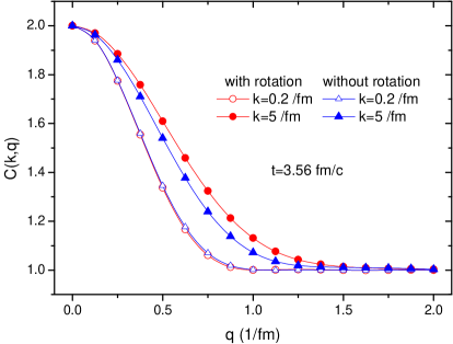
Figure 1: (color online) The dependence of the standard correlation function in the $\mbox{\boldmath$k$}_{+}$ direction from the collective flow, at the final time, 3.56 fm/c after reaching local equilibrium and 8.06 fm/c from the first touch, including the initial longitudinal expansion Yang-Mills field dynamics magas .

The fluid dynamical model is also able to describe emission in a ST volume or layer M-2 ; M-3 , or in hybrid models where a microscopic transport module is attached to the fluid dynamics, e.g. Yan12 . The determination of the FO surface normal or the emission direction from the ST FO layer and the emission profile in this layer are the subjects of present theoretical research, see AVC13 ; VAC13 ; Yun10 ; HP12 ; AVY13 . This complex FO process certainly has an influence on the HBT analysis, but our present aim is not to reproduce exactly a given experiment.

We focus on a single collective effect, the rotation, developing from the angular momentum during the initial stages of the fluid dynamics. Thus we constrain our discussion to the fluid dynamical stage, and adopt a relatively simple FO description from ref. Cso-5 , which can be implemented in Eq. (10). This provides the emission weight factors, $w_{s}$, which depend on the local mean emission direction $\hat{\sigma}^{\mu}$, and the flow velocity at the emission point.

The detector configuration is given by the two particles reaching a given detector in the direction of $k$. Thus the emission weights depend on the normal of the emission surface and of the emission, i.e. $\hat{\sigma}$ and $\hat{k}$. Most of the particles FO in a layer along a constant proper time hyperbola, with a dominant flow 4-velocity normal to this hyperbola: $\hat{\sigma}^{\mu}\approx u^{\mu}$. The origin of the hyperbola is at a ST point, which may precede the impact of the Lorentz contracted nuclei AVC13 .

We assume in the actual numerical calculations that in the expression of the weight, in Eq. (10), is the same for all surface layer elements: $Q_{s}^{(q)}=Q^{(q)}$ and $\Theta_{s}=\Theta$, so that $w_{s}=(k_{\mu}\,\hat{\sigma}^{\mu}_{s})\ \exp(-\Theta^{2}q_{0}^{2}/2)\ ,$ where $\hat{\sigma}_{s\mu}=(\sigma_{s}^{0},\mbox{\boldmath$\sigma$}_{s})$, so that $\ k_{\mu}\,\hat{\sigma}_{s}^{\mu}=k^{0}\sigma_{s}^{0}+\mbox{\boldmath$k$}\mbox{\boldmath$\sigma$}_{s}\ .$ If the emission path time-length, $\Theta$, tends to zero, then the time modifying factor becomes unity. With the choice $\hat{\sigma}_{\mu}=u_{\mu}$, the time-like FO normal is $\hat{\sigma}_{s\mu}=(\gamma_{s},\mbox{\boldmath$u$}_{s})$. Then $(k_{\mu}\hat{\sigma}^{\mu}_{s})=\gamma_{s}k_{0}{+}\mbox{\boldmath$k$}\mbox{\boldmath$u$}_{s}$. So the weight becomes

$$w_{s}=(\gamma_{s}k_{0}{+}\mbox{\boldmath$k$}\mbox{\boldmath$u$}_{s})\ \exp(-\Theta^{2}q_{0}^{2}/2).$$ (13)

This weight is explicitly different for the mirror image cell at $\mbox{\boldmath$x$}_{s}^{*}\rightarrow-\mbox{\boldmath$x$}_{s}$, where $\mbox{\boldmath$u$}_{s}^{*}\rightarrow-\mbox{\boldmath$u$}_{s}$ and then $w_{s}^{*}~{}=~{}(\gamma_{s}k_{0}{-}\mbox{\boldmath$k$}\mbox{\boldmath$u$}_{s})\exp(-\Theta^{2}q_{0}^{2}/2)\ .$

The weight factors appear both in the nominator and denominator of the correlator, so its normalization is balanced. On the other hand the role of the different factors in the weight have an effect to determine, which cells contribute more, which cells contribute less to the integrated result.

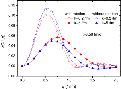
Figure 2: (color online) The Differential Correlation Function, $\Delta C(k,q)$, at the final time with and without rotation.

IV Results

The sensitivity of the standard correlation function on the fluid cell velocities decreases with decreasing distances among the cells. So, with a large number of densely placed fluid cells where all fluid cells contribute equally to the correlation function, the sensitivity on the flow velocity becomes negligibly weak.

Thus, the emission probability from different ST regions of the system is essential in the evaluation. This emission asymmetry due to the local flow velocity occurs also when the FO surface or layer is isochronous or if it happens at constant proper time.

We studied the fluid dynamical patterns of the calculations published in Ref. hydro2 , where the appearance of the KHI is discussed under different conditions. We chose the configuration, where both the rotation hydro1 , and the KHI occurred, at $b=0.7b_{max}$ with high cell resolution and low numerical viscosity at LHC energies, where the angular momentum is large, $L\approx 10^{6}\hbar$ VAC13 .

In spatially symmetric few source configurations CS13 , the standard correlation function did not show any difference if it is measured at two symmetric $k$ and $q$-out angles, e.g. in the reaction, [x-z] plane at $\mbox{\boldmath$k$}_{+}=(k_{x},0,+k_{z})$, $\mbox{\boldmath$q$}_{+}=(q_{x},0,+q_{z})$ and $\mbox{\boldmath$k$}_{-}=(k_{x},0,-k_{z})$, $\mbox{\boldmath$q$}_{-}=(q_{x},0,+q_{-})$, i.e. $\Delta C(k,q)$ vanished. Here we have chosen two directions at $\eta=\pm 0.76$, that is at polar angles of $90\pm 40$ degrees. These are measurable with the ALICE TPC and at the ATLAS and CMS also.

The standard correlation function is both influenced by the ST shape of the emitting source as well as its velocity distribution. The correlation function becomes narrower in $q$ with increasing time primarily due to the rapid expansion of the system. At the initial configuration the increase of $|\mbox{\boldmath$k$}|$ leads to a small increase of the width of the correlation function.

Nevertheless, in theoretical models we can switch off the rotation component of the flow, and analyse how the rotation influences the correlation function and especially the DCF, $\Delta C(k,q)$.

Fig. 1 compares the standard correlation functions with and without the rotation component of the flow at the final time moment. Here we see that the rotation leads to a small increase of the width in $q$ for the distribution at high values of $|\mbox{\boldmath$k$}|$, while at low momentum there is no visible difference.

In Fig. 2 $\Delta C(k,q)$ is shown for the configuration with and without rotation. For $k=5/$fm the rotation increases both the amplitude and the width of $\Delta C$. The dependence on $|\mbox{\boldmath$k$}|$ is especially large at the final time.

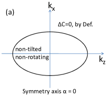
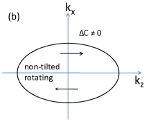
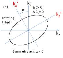
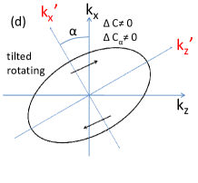
Figure 3: (Color online) Sketch of the configuration in different reference frames, with and without rotation of the flow. The non-rotating configurations have may have radial flow velocity components only. The DCF, $\Delta C_{\alpha}(k,q)$ is evaluated in a $K^{\prime}$ reference frame rotated by and angle $\alpha$ in the $x,z$, reaction plane. We search for the angle $\alpha$, where the non-rotataing configuration is ”symmetric”, so that it has a ”minimal” DCF as shown in Fig. 4.

In the original $K$ frame defined by the beam direction and the impact parameter, we can describe the vector $k$ with coordinates, $\mbox{\boldmath$k$}=\left\{\begin{array}[]{c}k_{x}\\ k_{z}\end{array}\right\}$. In the $K^{\prime}$ frame the same vector is then

$$\mbox{\boldmath$k$}^{\prime}(\alpha)=\left\{\begin{array}[]{c}k_{x^{\prime}}\\ k_{z^{\prime}}\end{array}\right\}=\left\{\begin{array}[]{c}k_{x}\cos\alpha-k_{z}\sin\alpha\\ k_{z}\cos\alpha+k_{x}\sin\alpha\end{array}\right\}\ .$$ (14)

Then one can define the DCF,

$$\Delta C_{\alpha}(\mbox{\boldmath$k$}^{\prime},\mbox{\boldmath$q$}^{\prime})\ ,$$ (15)

which depends on the angle $\alpha$. We have to find the proper symmetry axes of the emission ellipsoid. The conventional way would be the standard azimuthal HBT, however, we can exploit the features of the DCF. As the analytic examples CS13 show if (i) the shape is symmetric around the $x^{\prime}$ axis, and (ii) there is no rotation in the flow, then

$$\Delta C_{\alpha}\left(\mbox{\boldmath$k$}^{\prime},\mbox{\boldmath$q$}^{\prime}\right)=0\ .$$ (16)

Thus we can use the DFC to find the angle, $\alpha^{\prime}$, of the proper frame $K^{\prime}$ also. For a given $|\mbox{\boldmath$k$}|$ (e.g. $|\mbox{\boldmath$k$}|=5/$fm), we search for the minimum of the norm of the DCF as a function of $\alpha$.

This procedure is performed and the result is shown in Fig. 4 We separated the effect of the rotation by finding the symmetry angle where the rotation-less configuration yields vanishing or minimal $\Delta C$ for a given transverse momentum $k$.

The figure shows the result where the rotation component of the velocity field is removed. The DCF shows a minimum in its integrated value over $q$, for $\alpha=-11$ degrees. The shape of the DCF changes characteristically with the angle $\alpha$. Unfortunately this is not possible experimentally, so the direction of the symmetry axes should be found with other methods, like global flow analysis and/or azimuthal HBT analysis. To study the dependence on the angular momentum the same study was for lower angular momentum also, i.e. for a lower (RHIC) energy Au+Au collisions at the same impact parameter and time. We identified the angle where the rotation-less DCF was minimal, which was $\alpha=-8$ degrees, less than the deflection at higher angular momentum.

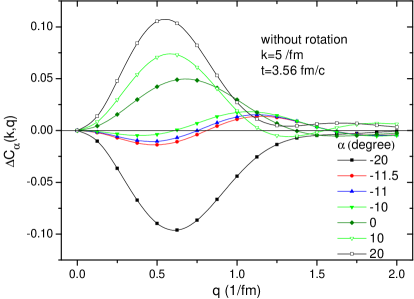
Figure 4: (Color online) The DCF at average pion wavenumber, $k=5/$fm and fluid dynamical evolution time, $t=3.56$fm/c, as a function of the functions of momentum difference in the ”out” direction $q$ (in units of 1/fm). The DCF is evaluated in a frame rotated in the reaction plane, in the c.m. system by angle $\alpha$.

We did this for two different energies, Pb+Pb / Au+Au at $\sqrt{s_{NN}}=2.36/0.2$ TeV respectively, while all other parameters of the collision were the same. The deflection angle of the symmetry axis was $\alpha=-11/-8$ degrees respectively. In these deflected frames we evaluated $\Delta C$ for the original, rotating configurations, which are shown in Fig. 5. This provides an excellent measure of the rotation.

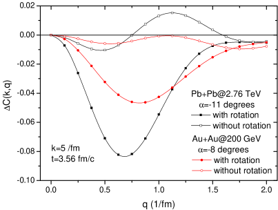
Figure 5: (color online) The DCF with and without rotation in the reference frames, deflected by the angle $\alpha$, where the rotation-less DCF is vanishing or minimal. In this frame the DCF of the original, rotating configuration indicates the effect of the rotation only. The amplitude of the DCF of the original rotating configuration doubles for the higher energy (higher angular momentum) collision.

On the other hand the rotation-less configuration cannot be generated from experimental data in an easy way. Other methods like the Global Flow Tensor analysis, or the azimuthal HBT analysis MLisa can provide an estimate for finding the deflection angle $\alpha$.

V Conclusion

The analysed model calculations show that the Differential HBT analysis can give a good quantitative measure of the rotation in the reaction plane of a heavy ion collision. These studies show that this measure is proportional to the beam energy or total angular momentum (while the polarization BCW2013 is not). It shows the best sensitivity at higher collective transverse momenta.

To perform the analysis in the rotation-less symmetry frame one can find the symmetry axis the best with the azimuthal HBT method, which provides even the transverse momentum dependence of this axis MLisa .

It is also important to determine the precise Event by Event c.m. position of the participants Eyyubova , and minimize the effect of fluctuations to be able to measure accurately the emission angles, which are crucial in the present $\Delta C(k,q)$ studies.

References

- (1) L.P. Csernai, V.K. Magas, H. Stöcker, and D.D. Strottman, Phys. Rev. C 84, 024914 (2011).
- (2) L.P. Csernai, D.D. Strottman and C. Anderlik, Phys. Rev. C 85, 054901 (2012).
- (3) L.P. Csernai, V.K. Magas, and D.J. Wang, Phys. Rev. C 87, 034906 (2013).
- (4) F. Becattini, L.P. Csernai, D.J. Wang, Phys. Rev. C 88, 034905 (2013).
- (5) Sz. Horvát, V.K. Magas, D.D. Strottman, L.P. Csernai, Phys. Lett. B 692, 277 (2010).
- (6) B. McInnes, and E.Teo, Nucl. Phys. B 878, 186 (2014).
- (7) V. Vovchenko, D. Anchishkin, and L.P. Csernai, Phys. Rev. C 88, 014901 (2013).
- (8) W. Florkowski: Phenomenology of Ultra-relativistic heavy-Ion Collisions, World Scientific Publishing Co., Singapore (2010).
- (9) A.N. Makhlin, Yu.M. Sinyukov, Z. Phys. C 39, 69 (1988); S.V. Akkelin, Yu.M. Sinyukov, Z. Phys. C 72, 501 (1996); T. Csörgő, S.V. Akkelin, Y. Hama, B. Lukács, and Yu.M. Sinyukov, Phys. Rev. C 67, 034904 (2003) .
- (10) L.P. Csernai, S. Velle, (2013) arXiv:1305.0385
- (11) T. Csörgő, Heavy Ion Phys. 15, 1-80, (2002); arXiv:hep-ph/0001233v3
- (12) E. Molnár, L. P. Csernai, V. K. Magas, Zs. I. Lazar, A. Nyiri, and K. Tamosiunas, J. Phys. G 34, 1901 (2007).
- (13) E. Molnár, L. P. Csernai, V. K. Magas, A. Nyiri, and K. Tamosiunas, Phys. Rev. C 74, 024907 (2006).
- (14) Yu-Liang Yan, Yun Cheng, Dai-Mei Zhou, Bao-Guo Dong, Xu Cai, Ben-Hao Sa, and Laszlo P Csernai, J. Phys. G 40, 025102 (2013).
- (15) D. Anchishkin, V. Vovchenko, and L.P. Csernai, Phys. Rev. C 87, 014906 (2013).
- (16) Y. Cheng, L.P. Csernai, V.K. Magas, B.R. Schlei, and D. Strottman, Phys. Rev. C 81, 064910 (2010).
- (17) P. Huovinen, H. Petersen, Eur. Phys. J. A 48, 171 (2012)
- (18) D. Anchishkin, V. Vovchenko, and S. Yezhov, Int. J. Modern Phys. E 22 1350042 (2013).
- (19) V.K. Magas, L.P. Csernai, D.D. Strottman, Phys. Rev. C 64, 014901 (2001), and Nucl. Phys. A 712, 167-204 (2002).
- (20) M.A. Lisa, N.N. Ajitanand, J.M. Alexander, et al., Phys. Lett. B 496, 1 (2000); M.A. Lisa, U. Heinz, U.A. Wiedemann, Phys. Lett. B 489, 287 (2000); E. Mount, G. Graef, M. Mitrovski, M. Bleicher, M.A. Lisa, Phys. Rev. C 84, 014908 (2011); G. Graef, M. Bleicher, and M. Lisa, Phys. Rev. C 89, 014903 (2014).
- (21) L.P. Csernai, G. Eyyubova, V.K. Magas, Phys. Rev. C 86, 024912 (2012).