Differential HBT Method to Analyze Rotation

Abstract

Two particle correlations are studied in the reaction plane of peripheral relativistic heavy ion reactions where the initial state has substantial angular momentum. The earlier predicted rotation effect and Kelvin Helmholtz Instability, leads to space-time momentum correlations among the emitted particles. A specific combination of two particle correlation measurements is proposed, which can sensitively detect the rotation of the emitting system. Here the method is presented in simple few source models where the symmetries and the possibilities of the detection can be demonstrated in a transparent way.

I Introduction

Collective flow is one of the most dominant observable features in heavy ion reactions up to the highest available energies, and its global symmetries as well as its fluctuations are extensively studied. Especially at the highest energies for peripheral reaction the angular momentum of the initial state is substantial, which leads to observable rotation according to fluid dynamical estimates hydro1 . Furthermore the low viscosity quark-gluon fluid may lead to to initial turbulent instabilities, like the Kelvin Helmholtz Instability (KHI), according to numerical fluid dynamical estimates hydro2 , which is also confirmed in a simplified analytic model KHI-Wang . These turbulent phenomena further increase the rotation of the system, which also leads to a large vorticity and circulation of the participant zone. CMW12 . In ref. hydro2 it is estimated that the increased rotation can be observable via the increased $v_{1}$-flow, but the $v_{1}$ signal at high energies is weak, so other observables of the rotation are also needed.

The two particle correlation method is used to determine the space-time size of the system emitting the observed particles, thus providing valuable information on the exploding and expanding system at the freeze out stage of a heavy ion collision. This method is based on the Hanbury Brown and Twiss (HBT) method, originally used for the determination of the size of distant stars StarHBT . In heavy ion collisions the HBT method was used first for the same purpose, the determination of the system size FirstHBTs , but later also the ellipsoidal shape of the system and its tilt DM95 ; MLisa . It was also observed relatively early that the expansion of the system modifies the size estimates due to the collective radial flow velocity of the emitting system Pratt , while the effect of flow on two particle correlations was also analysed in great detail Sin89 . Transport model studies have indicated that the HBT radius shows a minimum at the phase transition threshold QfLi07-9 .

A detailed two particle correlation study of flow rotation was not performed up to now LPSW . This became actual as at higher beam energies, where the initial angular momentum of the participant system is increasing in peripheral reactions, the system may rotate, causing a significant and detectable effect. Here we do not want to use the most advanced state of the art developments of the HBT method, rather we want to show in the most simple way, how rotation can be detected by the method.

Different theoretical approaches were worked out up to now to evaluate the two particle correlation functions in different reaction models. We here picked one method, which is not used very frequently up to now, but it can be generalized and used to fluid dynamical models with arbitrary flow patterns well. With this method hereby we study simplified, idealized fluid dynamical systems with different symmetry structures. These studies show how we can detect rotation via two particle correlation functions and what effects may cause difficulties in identifying rotation.

Based on these studies we also present a Differential Hanbury Brown and Twiss (DHBT) method, which can sensitively determine the strength (vorticity or circulation) of the rotating flow and the direction of this rotation.

I.1 The Emission Function

Following Cs-0 the definition of a particle 4-current is:

$$N^{\mu}=\int p^{\mu}\frac{d^{3}p}{p^{0}}f(x,p)\ ,$$ (1)

where $f(x,p)$ is the invariant scalar phase space density distribution of the emitted particles. The total flow of N nucleons across a space-time (ST) hypersurface, with the surface element, $d\sigma_{\mu}$ is:

$$N=\int\frac{d^{3}p}{p^{0}}\int d\sigma_{\mu}\,p^{\mu}f(x,p)\ .$$ (2)

If we do not perform the integration over the momentum, $p$, then we get the Cooper-Frye formula CF for invariant momentum distribution:

$$E\frac{dN}{d^{3}p}=\int d\sigma_{\mu}\,p^{\mu}f(x,p)\ ,$$ (3)

where $E=p^{0}$. This assumes that there is a 3-dimensional Freeze Out (FO) hypersurface, which can also be generalized to become a layer, as we will show. Using $d^{3}\mbox{\boldmath$p$}=dp_{||}d\mbox{\boldmath$p$}_{\perp}=p^{0}dyd\mbox{\boldmath$p$}_{\perp})$ we can write this in another form, and we can extend it to a 4-volume integral of a 4-dimensional Source Function, $S$, as CYW ; WF10 :

$$\frac{dN}{dyd^{2}p_{\perp}}=\int d\sigma_{\mu}(x)\,p^{\mu}f(x,p)=\int d^{4}x\,S(x,\mbox{\boldmath$p$})\ ,$$ (4)

where we assumed that the emission appears on a 3-dimensional hypersurface with the outward pointing normal, $d\sigma^{\mu}$. The emission function gives the distribution of the ST positions of momenta of emitted particles. The emission function gives the number of the particles, $\Delta N$, emitted in the phase-space element $\Delta^{3}x\Delta^{3}p$ per unit time, $\Delta t$. We get a Lorentz invariant scalar if we also multiply it by the energy, $p^{0}$, of the emitted particles:

$$S(x,\mbox{\boldmath$p$})=p^{0}\frac{\Delta N}{\Delta t\Delta^{3}x\Delta^{3}p}\ .$$ (5)

Along the lines of this introduction we can describe the emission over a hypersurface also as a 4-volume integral. We still assume a ST hypersurface with an outward pointing normal vector, $d\sigma^{\mu}$, but then the ST integral is interpreted as a 4-volume integral with a delta function for the given surface, $\delta(x^{\prime}-x)$ as:

$$\int S(x,\mbox{\boldmath$p$})\,d^{4}x=\int d^{4}x\,p^{\mu}\,\hat{\sigma}_{\mu}(x^{\prime})\,\delta^{(4)}(x^{\prime}-x)\,f(x,p)\ ,$$ (6)

where the emission is constrained to a 3-dimensional hypersurface in the ST and it is directed in a given direction characterized by the unit vector in the source described by $\hat{\sigma}_{\mu}(x^{\prime})\,\delta^{(4)}(x^{\prime})$. Even if we assume that the source is in a ST layer (which is not too thick, e.g. 2-3 fm or 2-3 fm/c), in this layer we can have a maximum of the emission. This FO layer in case of pions is narrow if we consider the rapid and simultaneous hadronization and FO from the plasma. This could even be idealized as a 3-dim hypersurface in the 4-dim ST if the thickness of the layer is neglected. Thus, $\hat{\sigma}_{\mu}$, is the unit normal vector of this surface or layer can be both timelike or spacelike:

$$\hat{\sigma}^{\mu}\hat{\sigma}_{\mu} = +1\ {\rm for\ timelike\ hypersurface\ or\ layer}\ ,$$

$$\hat{\sigma}^{\mu}\hat{\sigma}_{\mu} = -1\ {\rm for\ spacelike\ hypersurface\ or\ layer}\ .$$ (7)

The idealization of FO in a 3D hypersurface is not necessary, however it makes the presentation more transparent. The more realistic emission distribution must happen in a 4D ST surface layer, which can still can have an effective space-like or time-like normal vector. See refs. Sin89 ; M-2 ; M-3 ; M-4 . Although, one might naively believe that in case of a normal vector, $\hat{\sigma}^{\mu}=(1,0,0,0)$ the emission is uniform in all spatial directions, this is not true, as the local flow velocity also influences the emission probability Sin89 ; M-3 . When the flow velocity points in the direction of the detector (or the FO normal) the probability for the emission into the $\hat{\sigma}^{\mu}$-direction is bigger, so that the emission probability should be proportional to $(u^{\mu}\cdot\hat{\sigma}_{\mu})$. This will be important later on when the observability of rotation is discussed.

At ultrarelativistic energies most of the FO happens in time like directions, frequently idealized as $t=$constant or $\tau=$constant hypersurfaces or layers. In addition even in case of time-like FO the deeper (or earlier) points of the FO layer have a smaller emission probability because of the opacity of QGP, indicated also by the strong jet quenching. This effect causes additional asymmetries in the emission.

I.2 Hydrodynamical Parameterization

Let us assume that at the points of the source the matter is still in local equilibrium. Then we can describe the phase-space distribution of the particles, $f(x,p)$ by a Jüttner distributions Cs-0 or a relativistic Bose-Einstein or Fermi-Dirac distribution. Furthermore, instead of the delta function we may assume the emission distributed in a ST layer, which still has a preferred direction of emission $\hat{\sigma}^{\mu}$.

For our purposes the most suitable parametrization of the emission function is introduced in the special ”Buda-Lund” model, see section 8 of ref. Cso-5 . Here the emission function is parametrized as

$$S(x,\mbox{\boldmath$p$})\,d^{4}x=p^{\mu}\,d^{4}\Sigma_{\mu}(x)\,f(x,p),$$ (8)

where the emission probability and its dependence of the FO direction is already included in the $p^{\mu}\,d^{4}\Sigma_{\mu}(x)$ term. The 4-volume integral is directed and yields a maximum for $k^{\mu}$ which is closest to $d^{4}\Sigma^{\mu}(x)$. In the Buda-Lund model the FO direction points into the flow 4-velocity, $d^{4}\Sigma^{\mu}(x)\propto u^{\mu}$. This is also a frequent approximation in other fluid dynamical models, although, in the general case it is not a valid approximation. Thus, this approach is identical to the dynamical volume FO in a layer M-2 ; M-3 ; M-4 , discussed above. We also assume that the FO layer depends parametrically on the proper time, $\tau$, (or distance $s$) in the FO factor $d^{4}\Sigma^{\mu}(x)\propto\hat{\sigma}^{\mu}d^{4}x$. So, that the emission probability is proportional to  $G(x)\,H(\tau)$:

$$S(x,\mbox{\boldmath$p$})d^{4}x=p^{\mu}\ \hat{\sigma}_{\mu}(x)\ G(x)\,H(\tau)\,\ d\tau d^{3}x\ f(x,p)\ ,$$

where

$$H(\tau)=\frac{1}{(2\pi\Theta^{2})^{1/2}}\exp\left[-\frac{(\tau-\bar{\tau})^{2}}{2\Theta^{2}}\right],$$ (9)

and that the widths of the emitting sources do not change significantly during the course of emission from a given source. (The emission probability will be discussed in more detail when the source asymmetry is analysed in section III.) The emission function characterized with a locally thermalized volume-emitting source is then:

$$S(x,\mbox{\boldmath$p$})\,d^{4}x=\frac{g}{(2\pi\hbar)^{3}}\frac{p^{\mu}\,\hat{\sigma}_{\mu}(x)\,G(x)\,H(\tau)\,d\tau d^{3}x}{\exp\left(\frac{p^{\mu}u_{\mu}(x)}{T(x)}-\frac{\mu(x)}{T(x)}\right)-1},$$ (10)

where in place of $f(x,p)$ we inserted the relativistic Bose-Einstein distribution. The factor $g$ stands for the degeneracy, $u^{\mu}(x)$ is the 4-velocity field, $T(x)$ is the temperature field, $\mu(x)$ is the chemical potential and $d^{4}x=d\tau\,dx\,dy\,dz$. $G(x)$ is the ST emission density across the layer of the particles (e.g. pions). This can be approximated with a ST hypersurface and then with $\Theta\rightarrow 0$ we obtain the Cooper-Frye FO description. CF

For the phase space distribution we frequently use the Jüttner (relativistic Boltzmann) distribution:

$$f^{J}(x,p)=\frac{g}{(2\pi\hbar)^{3}}\exp\left(-\frac{p^{\mu}u_{\mu}(x)}{T(x)}+\frac{\mu(x)}{T(x)}\right),$$ (11)

which is normalized to the invariant scalar density of particles

$$n(x)=N^{\mu}u_{\mu}=u_{\mu}\int\frac{d^{3}p}{p^{0}}p^{\mu}\,f(x,p)=\frac{ge^{\mu/T}}{(2\pi\hbar)^{3}}C_{n},$$ (12)

where $C_{n}=4\pi m^{2}TK_{2}(m/T)$ and we use the $c=k=1$ convention. Thus in terms of the local invariant scalar particle density the Jüttner distribution is Cs-0

$$f^{J}(x,p)=\frac{n(x)}{C_{n}}\exp\left(-\frac{p^{\mu}u_{\mu}(x)}{T(x)}\right).$$ (13)

We can also define $d\sigma^{\mu}=dx\,dy\,dz\ \hat{\sigma}^{\mu}$ (for a timelike surface or layer) where the norm of $d\sigma^{\mu}$ is the 3-volume of the source element (like a fluid cell), similarly to Refs. M-2 ; M-3 ; M-4

Our source function in this case, with Eq. (13), similarly to Ref. Cso-5 in the frame where $\hat{\sigma}^{\mu}=(1,0,0,0)$ is:

$$G(x)=N_{FD}(x)/n(x),$$ (14)

where $N_{FD}(x)$ is the density of particles arising from fluid-dynamical (FD) evolution (or from other transport models). Then taking inti account the flow velocity in this frame:

$$N_{FD}(x)=\gamma n(x)\ .$$ (15)

The $H(\tau)$ (or $H(s)$) freeze-out probability along the $\tau$ (or $s$) parameter, across the layer can be integrated separately from the remaining three orthogonal coordinates.

Here we assume that the primary direction of the emission is $\hat{\sigma}^{\mu}$. Thus, in case of an explosively expanding system it points towards the detector, so $\hat{\sigma}^{\mu}\approx\hat{k}^{\mu}$. The emission happens from the 4-volume of ST surface layer with an effective normal direction $\hat{\sigma}^{\mu}$, and not from a ST hypersurface.

In ref. Sin89 the correlation function was analyzed in detail in dependence of the direction of the primary emission direction, $k^{\mu}$. A possibility of longitudinal momentum difference was considered in terms of the rapidity of the two emitted particles, where the difference of the longitudinal momenta, the width parameter, was studied in detail. While this analysis provides a deeper insight into the features of the correlation function, in our studies we concentrate to the rotation of the system and restrict ourself to a simplest presentation of the correlation function, which can be realized experimentally without much additional effort.

We can assume FO from a narrow layer at a proper time hyperbola $\tau_{FO}=cons.$ like in the Buda-Lund model, see ref. Cso-5 . This can be practical if the CFD model uses proper time and rapidity coordinates. Recent studies indicate that irrespective of the coordinate system choice, in the major part of FO in high energy collisions the FO happens near to a constant proper time hyperbola, although the origin of this FO-hyperbola is at an earlier point of time than the intersection of the centers of the projectile and target trajectories Anchiskin .

For the first test purpose we take an oversimplified model of 4 fluid elements, which may or may not expand or rotate. We assume that these are in the reaction plane, $[x-z]$-plane, and will characterise parameters of a heavy ion reaction based on CFD results. We assume that the system is stationary so the time emission probability is a Gaussian (like) distribution in time. Later on we intend to study and see that these methods can be applied for realistic full scale FD calculations also.

I.3 Pion Correlation Functions

The pion correlation function is defined as the inclusive two-particle distribution divided by the product of the inclusive one-particle distributions, such that WF10 :

$$C(p_{1},p_{2})=\frac{P_{2}(p_{1},p_{2})}{P_{1}(p_{1})P_{1}(p_{2})},$$ (16)

where $p_{1}$ and $p_{2}$ are the 4-momenta of the pions.

We will assume pions are created at two points, $x_{1}$ and $x_{2}$, which are distributed in space. The particle distribution is given by the reduced phase space source distribution:

$$S(x,{p})=f(x,{p})\,p^{\mu}\,\hat{\sigma}_{\mu}\,G(x)\,H(\tau)\ .$$ (17)

For two identical pions with momenta $p_{1}$ and $p_{2}$ the two-particle distribution is:

$$P_{2}(p_{1},p_{2})=\int d^{4}x_{1}d^{4}x_{2}S(x_{1},p_{1})S(x_{2},p_{2})|\psi_{12}|^{2},$$ (18)

where the wave equation $\psi_{12}$ is given by:

$$\psi_{12}=\frac{1}{\sqrt{2}}(e^{ip_{1}\cdot x_{1}+ip_{2}\cdot x_{2}}+e^{ip_{1}\cdot x_{2}+ip_{2}\cdot x_{1}})\ .$$ (19)

We now introduce the center-of-mass momentum

$$k=\frac{1}{2}(p_{1}+p_{2}),$$ (20)

and the relative momentum

$$q=p_{1}-p_{2},$$ (21)

where assuming the mass-shell constraint for the two particles and so we have $q\cdot k=(p_{1}-p_{2})\cdot(p_{1}+p_{2})/2=(p_{1}^{2}-p_{2}^{2})/2=(m_{\pi}^{2}-m_{\pi}^{2})/2=0$, which leads to $q^{0}=\mbox{\boldmath$q$}\cdot\mbox{\boldmath$k$}/k^{0}$

With the relative and center-of-mass momentum we can write the wave equation as:

$$\psi_{12}=\frac{e^{ik\cdot(x_{1}+x_{2})}}{\sqrt{2}}\left(e^{iq\cdot(x_{1}-x_{2})/2}+e^{-iq\cdot(x_{1}-x_{2})/2}\right)\ ,$$ (22)

and then

$$|\psi_{12}|^{2}=\left[1+\frac{1}{2}\left(e^{iq\cdot(x_{1}-x_{2})}+e^{-iq\cdot(x_{1}-x_{2})}\right)\right]\ .$$ (23)

We can then insert Eq. (23) into Eq. (18), and we obtain:

$$P_{2}(p_{1},p_{2}) = \int d^{4}x_{1}\,d^{4}x_{2}\,S(x_{1},{k}+{q}/2)\,S(x_{2},{k}-{q}/2)$$ (24)

$$\times \left[1+\frac{1}{2}\left(e^{iq\cdot(x_{1}-x_{2})}+e^{-iq\cdot(x_{1}-x_{2})}\right)\right]\ ,$$

where the last term in the brackets is $\cos[q(x_{1}-x_{2})]$. Similarly for the one particle distribution we get:

$$P_{1}(p)=\int d^{4}x\ S(x,k)\ .$$ (25)

We now use a method for moving sources presented in ref. Sinyukov-1 . Using Eqs. (24,25), together with the definition of the correlation function we have:

$$C(k,q)=1+\frac{R(k,q)}{\left|\int d^{4}x\,S(x,k)\right|^{2}}\ ,$$ (26)

where

$$\begin{split}R(k,q)=&\int d^{4}x_{1}\,d^{4}x_{2}\,\cos[q(x_{1}-x_{2})]\times\\ &S(x_{1},{k}+{q}/2)\,S(x_{2},{k}-{q}/2)\ .\end{split}$$ (27)

Here $R(k,q)$ can be calculated Sinyukov-1 via the function

$$\begin{split}&J(k,q)=\int d^{4}x\ S(x,k+q/2)\,\exp(iqx)=\\ &\int d^{4}x\ S(x,k+q/2)\,[\cos(qx)+i\sin(qx)]\ ,\end{split}$$ (28)

and we obtain the $R(k,q)$ function as

$$R(k,q)={\rm Re}\,[J(k,q)\,J(k,-q)]$$ (29)

This can be verified, by using Eq. (28), forming a double integral over $d^{4}x_{1}\,d^{4}x_{2}$ from $J(k,q)\,J(k,-q)$, yielding to a term $\exp[-iq(x_{1}-x_{2})]$. Then taking the real part of the double integral leads to a term $\cos[q(x_{1}-x_{2})]$ and this recovers Eq. (27).

Source with local Jütner distribution: Let us take the $S(x_{1},p_{1})S(x_{2},p_{2})$ term in Eq. (24), and assume that the single particle distributions, $f(x,p)$, in the source functions are Jüttner distributions, which depend on the local velocity, $u^{\mu}(x)$ , via the term

$$\exp\left(\frac{-p^{\mu}u_{\mu}(x)}{T(x)}\right)$$ (30)

as shown in Eq. (13). Here the local flow velocity may be different in different locations, $x_{1}$ and $x_{2}$, and this influences the correlations of the observed momenta. Thus, the scalar products in terms of $k$ and $q$ become:

$$\begin{split}&\exp(-p_{1}u_{1})\,\exp(-p_{2}u_{2})=\\ &\exp(-(k+q/2)\,u_{1})\,\exp(-(k-q/2)\,u_{2})=\\ &\exp(-ku_{1})\,\exp(-ku_{2})\,\exp(-q(u_{1}-u_{2})/2)\end{split}$$ (31)

where we used the notation $u_{1}=u(x_{1})=u^{\mu}(x_{1})$. We assume that for a given detector position the normal direction of the emission is approximately the same, so for the two sources the term $p^{\mu}\hat{\sigma}_{\mu}(x)\,$ is the same and it cancels in the nominator and denominator.

Thus, the expression of the correlation function, Eq. (27) will be modified to

$$\begin{split}R(k,q)=\int\!&d^{4}x_{1}d^{4}x_{2}\,S(x_{1},k)S(x_{2},k)\cos[q(x_{1}{-}x_{2})]\times\\ &\exp\left[-\frac{q}{2}\cdot\left(\frac{u(x_{1})}{T(x_{1})}-\frac{u(x_{2})}{T(x_{2})}\right)\right],\end{split}$$ (32)

and the corresponding $J(k,q)$ function will become

$$J(k,q)=\int d^{4}x\ S(x,k)\,\exp\left[-\frac{q\cdot u(x)}{2T(x)}\right]\,\exp(iqx)\ ,$$ (33)

In Eq. (32) the term including the momentum component $q$ and the flow velocity $u$ becomes unity if the source has a uniform distribution of $u(x)/T(x)$, and in this case we may be able to use the so called smoothness approximation: $S(x,k{+}q/2)S(y,k{-}q/2)\approx S(x,k)S(y,k)$, and the correlation function, expression (26), takes the form

$$C(k,q)=1+\frac{\left|\int d^{4}x\ e^{iqx}S(x,k)\right|^{2}}{\left|\int d^{4}x\,S(x,k)\right|^{2}}\ ,$$ (34)

I.4 One Fluid Cell as Source

We now assume a source function, which is reduced to one Freeze Out (FO) time moment. Thus the integration over the 4-volume of an emission layer is reduced to the 3-volume of a FO hypersurface. For simplicity, we assume FO along the timelike cordinate, $t$, where we assume a local Jüttner distribution. Thus, we have the source function as

$$S({x},k)=G(x)\,H(t)\exp\left(-\frac{k_{\mu}u^{\mu}(x)}{T(x)}\right)k^{\mu}\,\hat{\sigma}_{\mu}\ ,$$ (35)

where $k^{\mu}\hat{\sigma}_{\mu}$ is an invariant scalar, and for a single cell we use a simple quadratic parametrization for $n(x)$ as:

$$G(x)=\gamma n(x)=\gamma n_{s}\exp\left(-\frac{x^{2}+y^{2}+z^{2}}{2R^{2}}\right).$$ (36)

Here $n_{s}$ is the average density of the Gaussian source (or fluid cell) of mean radius $R$.

Single source at rest: The invariant scalar $k^{\mu}u_{\mu}$ can be calculated in the frame where the cell is at rest. We have then

$$u^{\mu}=(1,0,0,0)\Rightarrow-\frac{k_{\mu}u^{\mu}}{T}=-\frac{k^{0}}{T}=-\frac{E_{k}}{T}\ .$$ (37)

In this simplest case we also assume that the FO direction is $\hat{\sigma}^{\mu}=(1,0,0,0)$, so the $\tau$-coordinate coincides with the $t$-coordinate, and it is orthogonal to the $x,y,x-$ coordinates. Then we can make use of the following integral:

$$\int_{-\infty}^{+\infty}e^{-ax^{2}}d^{3}x=\left(\frac{\sqrt{\pi}}{\sqrt{a}}\right)^{3}\ .$$ (38)

We can perform the integral along the $t$ direction of $H(t)$, which gives unity and then the single particle distribution is

$$\begin{split}&\int\!d^{4}x\ S(x,k)=\frac{n_{s}}{C_{n}}\ (k^{\mu}\hat{\sigma}_{\mu})\ \exp\left(-\frac{E_{k}}{T_{s}}\right)\times\\ &\int_{-\infty}^{+\infty}\!\!\!\!\!\!H(t)dt\int_{-\infty}^{+\infty}\!\!\!\!e^{-\frac{x^{2}}{2R^{2}}}dx\int_{-\infty}^{+\infty}\!\!\!\!e^{-\frac{y^{2}}{2R^{2}}}dy\int_{-\infty}^{+\infty}\!\!\!\!e^{-\frac{z^{2}}{2R^{2}}}dz\ =\\ &n_{s}\ (k^{\mu}\hat{\sigma}_{\mu})\ \exp\left(-\frac{E_{k}}{T_{s}}\right)\frac{\left(2\pi R^{2}\right)^{3/2}}{C_{n}}\ ,\end{split}$$ (39)

where $T_{s}$ is the temperature of the source, and $E_{k}=k^{0}$ in the rest frame of the fluid cell. Due to the normalization of $H(t)$ the integral over the time $t$ is unity. The contribution to the nominator from Eq. (33) is

$$\begin{split}&J(k,q)=\int d^{4}x\,e^{iq\cdot x}e^{-q^{0}/(2T_{s})}S({x},k)\ =\ \frac{n_{s}\,(k^{\mu}\hat{\sigma}_{\mu})}{C_{n}}\ \times\\ &\exp\left[{-}\frac{E_{k}{+}q^{0}/2}{T_{s}}\right]\int_{-\infty}^{+\infty}\!\!\!\!\!\!\!H(t)e^{iq^{0}t}dt\int_{-\infty}^{+\infty}\!\!\!\!\!\!e^{{-\frac{x^{2}}{2R^{2}}}}e^{-iq_{x}x}dx\ \ \times\\ &\ \ \ \int_{-\infty}^{+\infty}\!\!\!\!\!e^{{-\frac{y^{2}}{2R^{2}}}}e^{-iq_{y}y}dy\int_{-\infty}^{+\infty}\!\!\!\!\!e^{{-\frac{z^{2}}{2R^{2}}}}e^{-iq_{z}z}dz=\\ &\frac{n_{s}(k^{\mu}\hat{\sigma}_{\mu})}{C_{n}}\left(2\pi R^{2}\right)^{3/2}\exp\left[{-}\frac{E_{k}}{T_{s}}\right]\exp\left[{-}\frac{q^{0}}{2T_{s}}\right]\times\\ &\ \ \ \exp\left[-\frac{R^{2}}{2}q^{2}\right]\exp\left[-\frac{\Theta^{2}}{2}(\hat{\sigma}^{\mu}q_{\mu})^{2}\right],\end{split}$$ (40)

where we used $\int_{-\infty}^{\infty}\exp(-p^{2}x^{2}{\pm}qx)dx=(\sqrt{\pi}/p)\times\exp(q^{2}/(4p^{2}))$ GR 3.323/2. In the time integral the present choice of $\hat{\sigma}^{\mu}$ would give $(q^{0})^{2}$, but we wanted to indicate that other choices are also possible and they would yield $(\hat{\sigma}^{\mu}q_{\mu})^{2}$. In the $J(k,q)J(k,-q)$ product the terms $\exp[\pm q^{0}/(2T_{s})]$ cancel each other. Inserting these equations into (26) we get

$$C(k,q)=1+\exp\left(-\Theta^{2}(\hat{\sigma}^{\mu}q_{\mu})^{2}-R^{2}q^{2}\right)\ .$$ (41)

If we have a source at a point in the FO layer, which is at a longer distance from the external side of the FO layer than $\Theta$, then the contribution of the time integral from this point is reduced. In a few source model it is more transparent to describe this reduction by assigning a smaller weight factor to the contribution of the deeper lying source. See in section III.

If we tend to an infinitely narrow FO layer, $\Theta\rightarrow 0$, i.e. to a FO hypersurface, then

$$C(k,q)=1+\exp\left(-R^{2}q^{2}\right)\ .$$ (42)

The $k$ dependence drops out from the correlation function, $C(k,q)$ as the $k$ dependent parts are separable. See Fig. 1. The size of the fluid cells in a high resolution 3+1D fluid dynamical calculation is $(0.3$fm$)^{3}$. With this resolution the numerical viscosity of the fluid dynamical calculation Horvat is the same as the estimated minimal viscosity of the QGP Kovtun which occurs at the critical point of the phase transition CsKM . As Fig. 1 shows the correlation for such a cell size yields to an extended distribution in the relative momentum $q$.

Figure 1: (color online) The correlation function, $C(k,q)$, for a single, static, spherically symmetric, Gaussian source with different radii, $R=4,1$ and $0.25$ fm, (blue dotted, red dashed, and full black lines respectively), as described by Eq. (42).

For the study of the rotation of the system the thickness of the FO layer is of secondary importance, especially if we discuss only a few fluid sources. In this case the role of the depth of a source point within the layer is given by its reduced contribution to the particle emission. This can be represented much simpler with assigning emission weights to the small number of sources. Thus, in the following discussion, we do not go into the details of the time structure of the emission.

Single moving source: Let us take a single source which moves in the x-direction with a velocity $v_{x}$. Then we have, $u_{s}^{\mu}=\gamma_{s}(1,v_{x},0,0)$, and the scalar product $k\cdot u_{s}/T_{s}=k_{\mu}u_{s}^{\mu}/T_{s}$ provides an additional contribution to the correlation function. However, in the case of a single fluid cell or a single source the velocity and the temperature do not change within the cell, so the modifying term in eq. (32) becomes unity. We use $k_{\mu}u^{\mu}=\gamma(E_{k}-k_{x}v_{x})$, and the source function becomes

$$S({x},k)=\frac{n(x)\,(k^{\mu}\,\hat{\sigma}_{\mu})}{C_{n}}\,\exp\left[-\frac{k\cdot u_{s}}{T_{s}}\right]\ ,$$ (43)

where $[k\cdot u_{s}/T_{s}]=[\gamma_{s}(E_{k}-k_{x}v_{x})/T_{s}]$.

Within the source (or fluid element) the velocity $u_{s}$ and temperature $T_{s}$ are assumed to be the same. The source or fluid element may have a density profile, but this profile should be the same for all cells (although the average density, $n_{s}$ is not the same for all cells. The spatial integrals can be performed in the rest frame of the cell, giving the same integral result as above (39), because the moving cell-size shrinks, but the apparent density increases, so that the total number of particles in a cell remains the same as it is an invariant scalar.

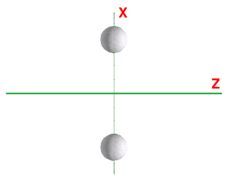
Figure 2: (color online) Two steady sources in the reaction ($[x-z]$) plane with a distance between them of $2d$ in the $x-$direction.

Then the integral of the single particle contribution is

$$\begin{split}\int\!d^{3}x\,S({x},k)\,&=\\ n_{s}(k^{\mu}\hat{\sigma}_{\mu})&\exp\left[-\frac{k\cdot u_{s}}{T_{s}}\right]\,\frac{\left(2\pi R^{2}\right)^{3/2}}{C_{n}}.\end{split}$$ (44)

Then the two particle distribution:

$$\begin{split}J(k,q)=\int\!d^{3}x\,e^{iq\cdot x}S({x},k)&\exp\left[-\frac{q\cdot u_{s}}{2T_{s}}\right]\,=\\ n_{s}(k^{\mu}\hat{\sigma}_{\mu})\exp\left[-\frac{k\cdot u_{s}}{T_{s}}\right]&\exp\left[-\frac{q\cdot u_{s}}{2T_{s}}\right]\times\\ \frac{\left(2\pi R^{2}\right)^{3/2}}{C_{n}}&\exp\left(-\frac{R^{2}}{2}q^{2}\right)\ .\end{split}$$ (45)

When calculating $R(k,q)$, in the $J(k,q)J(k,-q)$ product the terms $\exp[\pm q\cdot u_{s}/(2T_{s})]$ cancel each other. In the formulae the $\hbar=1$ convention is used and $k$ and $q$ are considered as the wavenumber vectors.

We then insert these equations into equation (26) and we get for one moving Gaussian source

$$C(k,q)=1+\exp\left(-R^{2}q^{2}\right)\ .$$ (46)

Again, this result does not depend on $k$, just as the previous single source at rest, Eq. (42).

II Symmetric Few Source Models

II.1 Two Steady Fluid Cells

For emission from two steady sources, two particle correlations were studied in ref. Cso-5 . Here we use the present method. We assume that the two source system is symmetric both their positions are placed symmetrically and also their FO normal vectors, $\hat{\sigma}^{\mu}$, are the same. If the normal were $\hat{\sigma}^{\mu}=(1,0,0,0)$, then the invariant scalar $k^{\mu}\hat{\sigma}_{\mu}$ would be $k^{0}=E_{k}$, although we do not need this additional requirement to illustrate the correlation function, which would arise from an idealized symmetric system.

We also assume that the time distributions, $H(\tau)$ for the two sources are identical, so these can be integrated simultaneously and yield unity. If we have two sources then the source function is

$$\begin{split}&S(x,k)=\sum_{s}S_{s}(x,k)=\\ &(k^{\mu}\hat{\sigma}_{\mu})\sum_{s}\frac{n_{s}(x)\,}{C_{ns}}\,\exp\left[-\frac{k\cdot u_{s}}{T_{s}}\right]\ ,\end{split}$$ (47)

while the $J$ function in the Jüttner approximation is

$$\begin{split}&J(k,q)=\\ &\sum_{s}\exp\left[-\frac{q\cdot u_{s}}{2T_{s}}\right]\,\exp(iqx_{s})\int_{S}d^{4}x\ S_{s}(x,k)\,\exp(iqx)\ ,\end{split}$$ (48)

where $x_{s}$ is the position of the center of the source, and the spatial integrals run separately for each of the identical sources, i.e. we assume fluid cells with identical density profiles, but with different densities, $n_{s}$ and temperatures, $T_{s}$.

In case of steady sources $u^{\mu}_{s}=(1,0,0,0)$, and the spatial integral for one source is the same as for a single source. Thus,

$$\begin{split}\int\!d^{3}x\ &S(x,k)=\sum_{s}\int_{S}d^{3}x\ S_{s}(x,k)=\\ &\left(2\pi R^{2}\right)^{3/2}\,(k^{\mu}\hat{\sigma}_{\mu})\sum_{s}\frac{n_{s}}{C_{ns}}\exp\left(-\frac{E_{k}}{T_{s}}\right)\end{split}$$ (49)

and

$$\begin{split}&J(k,q)=\\ &\sum_{s}\exp\left[-\frac{q^{0}}{2T_{s}}\right]\,\exp(iqx_{s})\int_{S}d^{3}x\ S_{s}(x,k)\,\exp(iqx)=\\ &\left(2\pi R^{2}\right)^{3/2}\ (k^{\mu}\hat{\sigma}_{\mu})\ \exp\left(-\frac{R^{2}}{2}q^{2}\right)\ \sum_{s}\frac{n_{s}}{C_{ns}}\ \times\\ &\exp\left(-\frac{E_{k}}{T_{s}}\right)\exp\left[-\frac{q^{0}}{2T_{s}}\right]\,\exp(iq^{0}x^{0}_{s})\exp(-i\mbox{\boldmath$q$}\mbox{\boldmath$x$}_{s})\ .\end{split}$$ (50)

In the $J(k,q)J(k,-q)$ product the terms $\exp[\pm q^{0}/(2T_{s})]$ cancel each other. Both $J(k,q)$ and $J(k,-q)$ include a sum $[\exp(i\mbox{\boldmath$q$}\mbox{\boldmath$x$}_{s})+\exp(-i\mbox{\boldmath$q$}\mbox{\boldmath$x$}_{s})]$, and their product leads to a factor $2[1+\cos(2\mbox{\boldmath$q$}\mbox{\boldmath$x$}_{s})]$. Here we assumed that the time-like extent of the emission layer is negligible compared to the space-like size.

Consequently, if the two sources have the same parameters, just different locations, $x_{1}=-x_{2}$ (see Fig. 2) then

$$C(k,q)=1+\frac{1}{2}\exp(-R^{2}q^{2})[1+\cos(2\mbox{\boldmath$q$}\mbox{\boldmath$x$}_{s})]$$ (51)

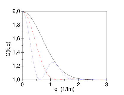
Figure 3: (color online) The correlation function, $C(k,q)$, for two spherical, Gaussian sources at rest, shown in the direction of the displacement (here $q_{x}$) with different distances, $d=2.5,1.25$ and $0$ fm, (dotted blue, dashed red, and full-black lines respectively) and in the orthogonal direction, $q_{y}$ which is identical with the $d=0$ contribution (full black line). For finite $d$ the cosine term results in a modification in the direction of the line joining the sources, which becomes apparent if the distance between the sources becomes small compared to the size of the spherical sources.

This result agrees with ref. Cso-5 , section 9.1 (p. 41), and in the limit of $\mbox{\boldmath$x$}_{s}=0$ it returns the single source result, Eq. (42). See Fig. 3. If the distance of the two sources is $2d$, i.e. $x_{1}=d$ and $x_{2}=-d$, then $2\mbox{\boldmath$q$}\mbox{\boldmath$x$}_{s}=2q_{x}\,d$, thus the modification appears in the $q_{x}$-direction only. In the other directions, $q_{y}$ and $q_{z}$, the single source result (42) is returned.

If the distance of the two sources, $2d$, is comparable or smaller than the radius of a single source, $R$, then the two source configuration leads to visible zero points, $C(k,q)=0$, on the $q_{x}$-axis at $2q_{x}\,d=\pm(1+2n)\pi$, where $n=0,1,2,3,...$   . In Fig. 3 for the $d=2.5$fm case we see these zero points at $q_{x}=\pi/(2d),3\pi/(2d)\,,\,$ … , while at the points $q_{x}=2\pi/(2d),4\pi/(2d)\,,\,$ … the distribution function, $C(k,q_{x})$ touches (becomes tangent to) the distribution function for $d=0$ or the distribution function $C(k,q_{y})$.

The appearance of the zero points is to a large extent an artifact of the used very simplistic two source model. In case of other additional sources these zero points would disappear. Nevertheless, this feature illustrates that the correlation function can be more complex than a set of Gaussians of the momentum difference $q$ in different directions or at different rapidities.

Figure 4: (color online) Two moving sources in the reaction ($[x-z]$) plane with a distance between them of $2d$ in the $x-$direction. The sources are moving in the directions indicated by the (red) arrows.

II.2 Two moving sources

We study the system the same way as before, but now the two sources are moving in opposite directions, so that $u_{s}=u_{1}$ or $u_{2}$ where $u_{1}^{\mu}=(\gamma_{s},\gamma_{s}\mbox{\boldmath$v$}_{1})$, $u_{2}=\bar{u}_{s}^{\mu}=(\gamma_{s},\gamma_{s}(-\mbox{\boldmath$v$}_{1}))$, and $\mbox{\boldmath$u$}_{s}\equiv\gamma_{s}\,\mbox{\boldmath$v$}_{s}$, so that $\mbox{\boldmath$u$}_{1}=-\mbox{\boldmath$u$}_{2}$, see Fig. 4. Similarly, $x_{s}=x_{1}$ or $x_{2}$ where $x_{s}^{\mu}=(t_{s},\mbox{\boldmath$x$}_{s})$, $\bar{x}_{s}^{\mu}=(t_{s},-\mbox{\boldmath$x$}_{s})$, and $\mbox{\boldmath$x$}_{1}=-\mbox{\boldmath$x$}_{2}$. For now we also assume that FO happens at a $t=$const. FO hypersurface, so $d\hat{\sigma}^{\mu}=(1,0,0,0)$ and so $t_{1}=t_{2}$.

If we have several sources then the source function in Jüttner approximation is

$$\begin{split}&S({x},k)=\sum_{s}S_{s}(x,k)=\\ &(k^{\mu}\,\hat{\sigma}_{\mu})\ \sum_{s}\frac{n_{s}(x)\,}{C_{ns}}\,\exp\left[-\frac{k\cdot u_{s}}{T_{s}}\right]\ ,\end{split}$$ (52)

while the $J$ function is

$$\begin{split}J(k,q)=&\sum_{s}\exp\left[-\frac{q\cdot u_{s}}{2T_{s}}\right]\times\\ &\exp(iqx_{s})\int_{S}d^{3}x\ S_{s}(x,k)\,\exp(iqx)\ ,\end{split}$$ (53)

where $x_{s}$ is the 4-position of the center of source $s$, and the spatial integrals run separately for each of the identical sources, i.e. we assume fluid cells with identical density profiles, but with different densities, $n_{s}$, velocities, $u_{s}$ and temperatures, $T_{s}$.

The spatial integral for one source is the same as for a single source. Thus,

$$\int\!d^{3}x\ S(x,k)=\sum_{s}\int_{S}d^{3}x\ S_{s}(x,k)=(k^{\mu}\,\hat{\sigma}_{\mu})\ \left(2\pi R^{2}\right)^{3/2}\ \ \frac{n_{s}}{C_{ns}}\exp\left(-\frac{k^{0}\gamma_{s}}{T_{s}}\right)\left[\exp\left(\frac{\mbox{\boldmath$k$}\mbox{\boldmath$u$}_{s}}{T_{s}}\right)+\exp\left(-\frac{\mbox{\boldmath$k$}\mbox{\boldmath$u$}_{s}}{T_{s}}\right)\right]\ .$$ (54)

This returns Eq. (49) if $u^{\mu}_{s}=(1,0,0,0)$. The function $J(k,q)$ becomes

$$\begin{split}&J(k,q)=\sum_{s}\exp\left[-\frac{q\cdot u_{s}}{2T_{s}}\right]\,\exp(iqx_{s})\int_{S}d^{4}x\ S_{s}(x,k)\,\exp(iqx)=\\ &(k^{\mu}\,\hat{\sigma}_{\mu})\ \left(2\pi R^{2}\right)^{3/2}\exp\left(-\frac{R^{2}q^{2}}{2}\right)\sum_{s}\frac{n_{s}}{C_{ns}}\exp\left[-\frac{k\cdot u_{s}}{T_{s}}\right]\exp\left[-\frac{q\cdot u_{s}}{2T_{s}}\right]\,\exp(iqx_{s})=\\ &(k^{\mu}\,\hat{\sigma}_{\mu})\ \left(2\pi R^{2}\right)^{3/2}\exp\left(-\frac{R^{2}}{2}q^{2}\right)\frac{n_{s}}{C_{ns}}\exp\left[-\frac{k^{0}\gamma_{s}}{T_{s}}\right]\exp\left[-\frac{q^{0}}{2}\frac{\gamma_{s}}{T_{s}}\right]\exp(iq^{0}x_{s}^{0})\times\\ &\left[\exp\left[\frac{\mbox{\boldmath$k$}\mbox{\boldmath$u$}_{s}}{T_{s}}\right]\exp\left[\frac{\mbox{\boldmath$q$}\mbox{\boldmath$u$}_{s}}{2T_{s}}\right]\exp(-i\mbox{\boldmath$q$}\mbox{\boldmath$x$}_{s})+\exp\left[-\frac{\mbox{\boldmath$k$}\mbox{\boldmath$u$}_{s}}{T_{s}}\right]\exp\left[-\frac{\mbox{\boldmath$q$}\mbox{\boldmath$u$}_{s}}{2T_{s}}\right]\exp(i\mbox{\boldmath$q$}\mbox{\boldmath$x$}_{s})\right],\end{split}$$ (55)

where the factor $\exp(iq^{0}x_{s}^{0})$ can be dropped if the FO time distribution is simultaneous for the two sources, because then $x_{s}^{0}=0$. This returns Eq. (50) if $u^{\mu}_{s}=(1,0,0,0)$.

Now we can divide the two particle correlation with the square of the single particle distribution

$$\begin{split}\frac{Re\,[J(k,q)\,J(k,-q)]}{\left|\int d^{4}x\,S(x,k)\right|^{2}}&\ \ =\ \ \exp(-R^{2}q^{2})\frac{Re\left[e^{\frac{2\mbox{\boldmath$k$}\mbox{\boldmath$u$}_{s}}{T_{s}}}+e^{-\frac{2\mbox{\boldmath$k$}\mbox{\boldmath$u$}_{s}}{T_{s}}}+e^{\frac{\mbox{\boldmath$q$}\mbox{\boldmath$u$}_{s}}{T_{s}}}e^{i2\mbox{\boldmath$q$}\mbox{\boldmath$x$}_{s}}+e^{-\frac{\mbox{\boldmath$q$}\mbox{\boldmath$u$}_{s}}{T_{s}}}e^{-i2\mbox{\boldmath$q$}\mbox{\boldmath$x$}_{s}}\right]}{\left(e^{\frac{\mbox{\boldmath$k$}\mbox{\boldmath$u$}_{s}}{T_{s}}}+e^{-\frac{\mbox{\boldmath$k$}\mbox{\boldmath$u$}_{s}}{T_{s}}}\right)^{2}}\\ =\exp(-R^{2}q^{2})&\frac{\ Re\,\left[2\cosh\left(\frac{2\mbox{\boldmath$k$}\mbox{\boldmath$u$}_{s}}{T_{s}}\right)+e^{\frac{\mbox{\boldmath$q$}\mbox{\boldmath$u$}_{s}}{T_{s}}}\left(\cos(2\mbox{\boldmath$q$}\mbox{\boldmath$x$}_{s})+i\sin(2\mbox{\boldmath$q$}\mbox{\boldmath$x$}_{s})\right)+e^{-\frac{\mbox{\boldmath$q$}\mbox{\boldmath$u$}_{s}}{T_{s}}}\left(\cos(-2\mbox{\boldmath$q$}\mbox{\boldmath$x$}_{s})+i\sin(-2\mbox{\boldmath$q$}\mbox{\boldmath$x$}_{s})\right)\right]}{2\left[\cosh\left(\frac{2\mbox{\boldmath$k$}\mbox{\boldmath$u$}_{s}}{T_{s}}\right)+1\right]}\\ =\exp(-R^{2}q^{2})&\frac{\cosh\left(\frac{2\mbox{\boldmath$k$}\mbox{\boldmath$u$}_{s}}{T_{s}}\right)+\cosh\left(\frac{\mbox{\boldmath$q$}\mbox{\boldmath$u$}_{s}}{T_{s}}\right)\cos(2\mbox{\boldmath$q$}\mbox{\boldmath$x$}_{s})}{\cosh\left(\frac{2\mbox{\boldmath$k$}\mbox{\boldmath$u$}_{s}}{T_{s}}\right)+1}\\ \end{split}$$ (56)

Consequently, if the two sources have the same parameters, just opposite locations with respect to the center, and opposite velocities, then the correlation function is

$$\begin{split}C(k,q)&=1+\exp(-R^{2}q^{2})\ \times\\ &\frac{\cosh\left(\frac{2\mbox{\boldmath$k$}\mbox{\boldmath$u$}_{s}}{T_{s}}\right)+\cosh\left(\frac{\mbox{\boldmath$q$}\mbox{\boldmath$u$}_{s}}{T_{s}}\right)\cos(2\mbox{\boldmath$q$}\mbox{\boldmath$x$}_{s})}{\cosh\left(\frac{2\mbox{\boldmath$k$}\mbox{\boldmath$u$}_{s}}{T_{s}}\right)+1}\ .\end{split}$$ (57)

This returns Eq. (51) if $u^{\mu}_{s}=(1,0,0,0)$, and $C(k,q)=2$ if $q=0$.

If we have two sources placed at $x=\pm d_{x}$, and with the velocity in the $\pm z$-direction, $\pm v_{z}$, then the correlation function is for the different directions becomes:

$$\begin{split}C(k_{x},q_{x})&=1+\frac{1}{2}\exp(-R^{2}q^{2}_{x})\left[1+\cos\left(2q_{x}d_{x}\right)\right]\ ,\\ C(k_{x},q_{y})&=1+\exp(-R^{2}q^{2}_{y})\ ,\\ C(k_{x},q_{z})&=1+\frac{\exp(-R^{2}q^{2}_{z})}{2}\left[1+\cosh\left(\frac{\gamma q_{z}v_{z}}{T_{s}}\right)\right]\ .\end{split}$$ (58)

$$\begin{split}C(k_{y},q_{x})&=1+\frac{1}{2}\exp(-R^{2}q^{2}_{x})\left[1+\cos\left(2q_{x}d_{x}\right)\right]\ ,\\ C(k_{y},q_{y})&=1+\exp(-R^{2}q^{2}_{y})\ ,\\ C(k_{y},q_{z})&=1+\frac{\exp(-R^{2}q^{2}_{z})}{2}\left[1+\cosh\left(\frac{\gamma q_{z}v_{z}}{T_{s}}\right)\right]\ .\end{split}$$ (59)

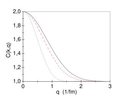
Figure 5: (color online) The correlation functions, $C(k,q)$, for two moving sources where the displacement of the sources is in the $x$-direction, and the center-of-mass momentum, $k$, of emitted particles is in the $x$ and $y$ direction. The solid black line is for the momentum difference, $q_{z}$, the dashed red line is for $q_{y}$ and dotted blue line is for $q_{x}$. The radius of the sources is $R=1$ fm, (same as in Fig. 3), the displacement is $d=1$fm, and the source velocity is, $\gamma v_{z}/T_{s}=1.0$ fm. This can be satisfied e.g. by $u_{s}=0.6$ c and $T=0.12$ GeV.

$$\begin{split}C(k_{z},q_{x})=\ &1+\exp(-R^{2}q^{2}_{x})\ \times\\ &\frac{\cosh\left(\frac{2\gamma k_{z}v_{z}}{T_{s}}\right)+\cos\left(2q_{x}d_{x}\right)}{\cosh\left(\frac{2\gamma k_{z}v_{z}}{T_{s}}\right)+1}\ ,\\ C(k_{z},q_{y})=\ &1+\exp(-R^{2}q^{2}_{y})\ ,\\ C(k_{z},q_{z})=\ &1+\exp(-R^{2}q^{2}_{z})\ \times\\ &\frac{\cosh\left(\frac{2\gamma k_{z}v_{z}}{T_{s}}\right)+\cosh\left(\frac{\gamma q_{z}v_{z}}{T_{s}}\right)}{\cosh\left(\frac{2\gamma k_{z}v_{z}}{T_{s}}\right)+1}\ .\end{split}$$ (60)

Therefore only the correlation functions in the $k_{z},q_{x}$-direction and in the $q_{z}$-directions are affected by the $z$-directed velocity of the source. In this direction, $k_{z}$, unfortunately it is difficult to detect the two particle correlations. For the $k_{x}$ and $k_{y}$-directions the $q_{x}$-distribution is affected by the displacement of the two sources by $\pm d_{x}$. The $q_{y}$-distribution is not effected by either the displacement or the source velocities.

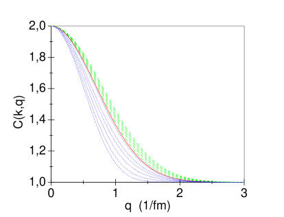
Figure 6: (color online) The correlation functions, $C(k,q)$ for two moving sources where the displacement of the sources is in the $z$-direction, and the center-of-mass momentum, $k$, of emitted particles is in the $x$-direction. The dashed green lines are for the relative momentum, $q_{z}$, the solid red line is for $q_{y}$ and dotted blue lines are for $q_{x}$. For large values of the center-of-mass momentum $k_{x}$ the correlation functions $C(k_{x},q_{x})$ and $C(k_{x},q_{z})$ will approach the correlation function $C(k_{x},q_{y})$  (red line). For $q_{x}$ (blue lines) the displacements are $d_{x}=1,0$ fm, and for $q_{z}$ (green lines) the velocity is chosen such that $\gamma v_{z}/T_{s}=1.0$ fm. The values of $k_{z}$ are for the blue lines: 0.25, 0.5, 0.75, 1.0, 1.25 and 2.0 fm^-1 and for the green lines: 0.25, 0.5, 0.75, 1.0 and 1.5 fm^-1.

The correlation function for different source locations and velocities are similar. The cosine term appears in the same direction as the axis at which the sources are located and the hyperbolic cosine in the direction of the velocity. See Figs. 5 and 6. The zero points discussed for the two static sources at Eq. (51), appear in the distributions $C(k_{x},q_{x})$ and $C(k_{y},q_{x})$. These distributions do depend on the magnitude of the flow velocity, $v_{z}$, but not on its direction! This arises from the fact that the detectors are assumed to be reached from both sides of the system with opposite velocities with equal probability.

Unfortunately the dominant direction of flow (see Fig. 8) is the beam direction ($z-$direction), where we have no possibility to place high acceptance detectors. At the same time the strongest effect of the flow appears in this direction.

The rotation in the reaction plane can also be characterized with another configuration of the two moving sources, when the displacement is in the $z$-direction while the flow velocities are pointing into the $x$-direction, so that the source at $x_{1}=d_{z}$ has a negative velocity, $-v_{x}$ while the source at $x_{2}=-d_{z}$ has a positive velocity, $v_{x}$. (See Fig. 7.) The detailed description of the correlation functions from this configuration can be obtained in a straightforward way similarly to the previous case, see Eq. (61). In this case the flow has the most dominant effect in the $k_{x}$-direction, which is accessible for detection. The $x$-directed flow, however, is more sensitively dependent on secondary effects, like the Kelvin-Helmholtz Instability hydro2 .

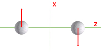
Figure 7: (color online) Two moving sources in the reaction ($[x-z]$) plane with a distance between them of $2d$ in the $z-$direction. The sources are moving in the directions indicated by the (red) arrows.

In this configuration of the sources the magnitude of the flow velocity makes visible change in $C(k,q)$, in the $(k_{x},q_{x})$-direction also, which is detectable by the usual detector configurations. Still the direction of the rotation does not appear in the observables with the approach presented here.

This actually arises from the simplifying assumption, that the freeze out is happening instantly at a timelike hypersurface with $\hat{\sigma}^{\mu}=(1,0,0,0)$, where particles from all sides of the system can reach each detector with the same probability. We will return to this problem after having discussed the more complex source configurations.

$$\begin{split}C(k_{x},q_{x})=\ &1+\exp(-R^{2}q^{2}_{x})\ \times\\ &\frac{\cosh\left(\frac{2\gamma k_{x}v_{x}}{T_{s}}\right)+\cosh\left(\frac{\gamma q_{x}v_{x}}{T_{s}}\right)}{\cosh\left(\frac{2\gamma k_{x}v_{x}}{T_{s}}\right)+1}\ ,\\ C(k_{x},q_{y})=\ &1+\exp(-R^{2}q^{2}_{y})\ ,\\ C(k_{x},q_{z})=\ &1+\exp(-R^{2}q^{2}_{z})\ \times\\ &\frac{\cosh\left(\frac{2\gamma k_{x}v_{x}}{T_{s}}\right)+\cos\left(2q_{z}d_{z}\right)}{\cosh\left(\frac{2\gamma k_{x}v_{x}}{T_{s}}\right)+1}\ .\end{split}$$ (61)

For these two-particle correlation measurements it is necessary to identify independently, event by event the global collective reaction plane azimuth, $\Psi_{RP}$, experimentally and the corresponding event by event center of mass of the system (e.g. with the method Eyyubova ). Knowing these we can identify the $k_{x}$-direction (and the $k_{y}$-direction also.

In this section we derived a relatively simple formula for two sources with opposite positions and opposite velocities. These kind of systems were analysed earlier for radially expanding systems.

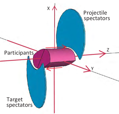
Figure 8: (Color online) Typical orientation of the spatial axes in case of an ultra-relativistic heavy ion reaction shortly after the impact. In the configuration space the projectile and target appear to be flat due to the Lorentz contraction.

Recently due to the angular momentum in peripheral heavy ion collisions strong rotation hydro1 and turbulence (Kelvin-Helmholtz Instability) hydro2 were predicted in fluid dynamical models arising from the symmetries, shear and vorticity of the initial state.

In the simple two source example shown in the previous section the two sources may describe a rotation if the sources are at a distance from the center in the x-direction, $\mbox{\boldmath$x$}_{1}=(+d,0,0)$ and $\mbox{\boldmath$x$}_{2}=(-d,0,0)$, while these have opposite velocities pointing into the z-direction, $\mbox{\boldmath$u$}_{1}=\gamma(1,0,0,v_{z})$ and $\mbox{\boldmath$u$}_{2}=\gamma(1,0,0,-v_{z})$.

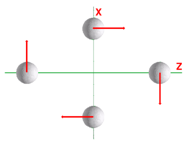
Figure 9: (color online) Four moving sources in the reaction ($[x-z]$) plane, one pair, $s1$, is separated in the $x-$ directions and the other, $s2$, is in the $z-$ direction. The sources are moving in the directions indicated by the (red) arrows, $\pm\mbox{\boldmath$u$}_{s1}$ for the 1st pair and $\pm\mbox{\boldmath$u$}_{s2}$ for the other.

It is important to mention that to detect rotation the accurate identification of the reaction plane and its proper orientation is necessary. In the so called ”cumulative” methods the reaction plane is identified but its projectile and target sides are not. This makes it impossible to detect directed flow, and odd components of the global collective flow. (All harmonic components of random fluctuations of course can be detected.) Furthermore, not only the reaction plane with proper direction but also the event by event center of mass (c.m.) should also be identified Eyyubova . This hardly ever done! In both cases the use of zero degree calorimeters are provide an adequate tool as these are sensitive to the spectator residues.

The correlation function depends both on vectors $k$ and $q$. To detect rotation the choices should be correlated correctly with the beam and the directed reaction plane as illustrated in Fig. 8. The positive x-axis points in the direction of the projectile, which moves in the positive direction along the z-axis.

In Eq. (57), in the above situation, $\mbox{\boldmath$k$}\mbox{\boldmath$u$}_{s}=\gamma k_{z}v_{z}$,   $\mbox{\boldmath$q$}\mbox{\boldmath$u$}_{s}=\gamma q_{z}v_{z}$   and $\mbox{\boldmath$q$}\mbox{\boldmath$x$}_{s}=q_{x}d$. Thus, the Correlation function, apart of the single cell source size, $R$, sensitivity, has a specific dependence on $k_{z}$ and $q_{z}$, as well as on $q_{x}$. Unfortunately it is difficult to measure the particle momenta in the z-direction as it coincides with the beam. The $q_{x}$ dependence would enable us to estimate the distance of the two sources.

II.3 Four Fluid Cell Sources

Four sources can be treated as a combination of two moving double source systems. We use the same parameters as under paragraph II.2, where $s_{1}$ and $s_{2}$ will be the two different pairs of sources with different locations and velocities. See Fig. 9.

So we have

$$\begin{split}C(k,q)&=1+\exp(-R^{2}q^{2})\times\\ &\left[\cosh\left(\frac{2\mbox{\boldmath$k$}\cdot\mbox{\boldmath$u$}_{s_{1}}}{T_{s}}\right)+\cosh\left(\frac{\mbox{\boldmath$q$}\cdot\mbox{\boldmath$u$}_{s_{1}}}{T_{s}}\right)\cos(2\mbox{\boldmath$q$}\cdot\mbox{\boldmath$x$}_{s_{1}})+\cosh\left(\frac{2\mbox{\boldmath$k$}\cdot\mbox{\boldmath$u$}_{s_{2}}}{T_{s}}\right)+\cosh\left(\frac{\mbox{\boldmath$q$}\cdot\mbox{\boldmath$u$}_{s_{2}}}{T_{s}}\right)\cos(2\mbox{\boldmath$q$}\cdot\mbox{\boldmath$x$}_{s_{2}})+\right.\\ &2\cosh\left(\frac{\mbox{\boldmath$k$}\cdot(\mbox{\boldmath$u$}_{s_{1}}-\mbox{\boldmath$u$}_{s_{2}})}{T_{s}}\right)\cosh\left(\frac{\mbox{\boldmath$q$}\cdot(\mbox{\boldmath$u$}_{s_{1}}+\mbox{\boldmath$u$}_{s_{2}})}{2T_{s}}\right)\cos(\mbox{\boldmath$q$}\cdot(\mbox{\boldmath$x$}_{s_{1}}+\mbox{\boldmath$x$}_{s_{2}}))+\\ &\left.2\cosh\left(\frac{\mbox{\boldmath$k$}\cdot(\mbox{\boldmath$u$}_{s_{1}}+\mbox{\boldmath$u$}_{s_{2}})}{T_{s}}\right)\cosh\left(\frac{\mbox{\boldmath$q$}\cdot(\mbox{\boldmath$u$}_{s_{1}}-\mbox{\boldmath$u$}_{s_{2}})}{2T_{s}}\right)\cos(\mbox{\boldmath$q$}\cdot(\mbox{\boldmath$x$}_{s_{1}}-\mbox{\boldmath$x$}_{s_{2}}))\right]\times\\ &\left[\cosh\left(\frac{2\mbox{\boldmath$k$}\cdot\mbox{\boldmath$u$}_{s_{1}}}{T_{s}}\right)+\cosh\left(\frac{2\mbox{\boldmath$k$}\cdot\mbox{\boldmath$u$}_{s_{2}}}{T_{s}}\right)+2\cosh\left(\frac{\mbox{\boldmath$k$}\cdot(\mbox{\boldmath$u$}_{s_{1}}+\mbox{\boldmath$u$}_{s_{2}})}{T_{s}}\right)+2\cosh\left(\frac{\mbox{\boldmath$k$}\cdot(\mbox{\boldmath$u$}_{s_{1}}-\mbox{\boldmath$u$}_{s_{2}})}{T_{s}}\right)+2\right]^{-1}\\ \end{split}$$ (62)

If $s_{1}=s_{2}$ then we recover Eq. (57)

In the case of a rotating but symmetric system the displacements and velocities are of equal magnitude and are orthogonal to each other in the two pairs: $\mbox{\boldmath$x$}_{s_{1}}\perp\mbox{\boldmath$x$}_{s_{2}}$ and $\mbox{\boldmath$u$}_{s_{1}}\perp\mbox{\boldmath$u$}_{s_{2}}$. Thus a simple sign change of the velocity for one of the pairs or both does not change the result, and so the rotation can be identified, but this evaluation does not provide sensitivity to the direction of the rotation. The reason is in the simplified freeze out assumption as we mentioned already at the end of paragraph II.2.

If the two pairs are not completely identical, i.e. the magnitude of the characteristic quantities of the two source pairs are not equal then a sensitivity to the direction of the rotation may in principle occur. However, if we change the direction of the velocities of the two source pairs simultaneously (as it happens in changing the direction of rotation) the result still does not change.

Four Sources with Flow Circulation: Recent fluid dynamical studies indicate hydro1 ; hydro2 , that due to the initial shear and angular momentum the early fluid dynamical development has significant flow vorticity and circulation on the reaction plane. These were recently evaluated CMW12 . At the present LHC Pb+Pb collision energy in the mentioned fluid dynamical model calculation the maximum value of vorticity, $\omega$, was found exceeding $3$ c/fm , and the circulation after $6$ fm/c flow development and expansion was still around 4-5 fm$\cdot$c. This vorticity in the reaction plane was more than an order of magnitude bigger than in the transverse plane estimated from random fluctuations in ref. FW11 .

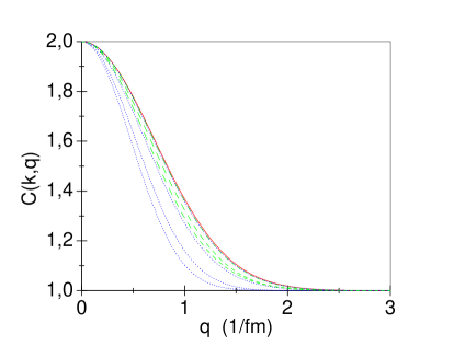
Figure 10: (color online) The correlation functions, $C(k,q)$, for 4 sources where the displacement is such that there is one source pair on the x-axis and one the z-axis, the center-of-mass momentum of the emitted particles, $k$, is in the x-direction. The dotted blue lines are for the velocity $v=0.5$ c and displacement $d_{x}=d_{z}=1.6$ fm. The dashed green lines are for the velocity $v=0.8$ c and displacement $d_{x}=d_{z}=1.0$ fm. $T_{s}=0.20$ GeV. In both cases the circulation is $\Gamma=5$ fm$\cdot$c. The values of $k_{x}$ are for the blue lines: 0.5, 1.5, 3.0 and 6.0 fm^-1 and for the green lines: 0.5, 1.5 and 3.0 fm^-1. The solid red line is the correlation function $C(k_{x},q_{y})$. For large values of the center-of-mass momentum $k_{x}$ the correlation functions $C(k_{x},q_{x})$ and $C(k_{x},q_{z})$ will approach the correlation function $C(k_{x},q_{y})$. The larger displacement and smaller rotation velocity leads to stronger deviation from the unaffected correlation function $C(k_{x},q_{y})$.

In this section we will look at the four source correlation function with similar circulation as in the above mentioned fluid dynamical model estimates in the reaction plane. See Fig. 9. We will simulate a circulation value $\Gamma=5fm\cdot c$. We use Eq. (62) where the center-of-mass momentum, $k$ points in the $x-direction$.

Since the position and velocity are of the same value and because of symmetry the correlation functions $C(k_{x},q_{x})$ and $C(k_{x},q_{z})$ provide the same values. So we take the correlation function $C(k_{x},q_{x})$ and we have afterwards some simplifications. See Fig. 10.

$$\begin{split}&C(k_{x},q_{x})=1+\exp(-R^{2}q^{2})\times\\ &\left[1+\cos(2q_{x}d)+\cosh\left(2\frac{k_{x}\gamma v_{x}}{T_{s}}\right)+\cosh\left(\frac{q_{x}\gamma v_{x}}{T_{s}}\right)+\right.\\ &\left.4\cosh\left(\frac{k_{x}\gamma v_{x}}{T_{s}}\right)\cosh\left(\frac{q_{x}\gamma v_{x}}{2T_{s}}\right)\cos(q_{x}d)\right]\times\\ &\left[\cosh\left(\frac{2k_{x}\gamma v_{x}}{T_{s}}\right)+4\cosh\left(\frac{k_{x}\gamma v_{x}}{T_{s}}\right)+3\right]^{-1}\end{split}$$ (63)

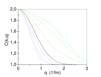
Figure 11: (color online) The correlation functions, $C(k,q)$, for 4 sources where the displacement is such that there is one source pair on the x-axis and one the z-axis, the center-of-mass momentum of the emitted particles, $k$, is in the x-direction. The dotted blue lines are for the velocity $v=0.5$ c and displacement $d_{x}=d_{z}=1.6$ fm (same as in the previous figure). The dashed green lines are for the velocity $v=0.95$ c and displacement $d_{x}=d_{z}=0.84$ fm, $T_{s}=0.20$ GeV. The values of $k_{x}$ are: for the blue lines 0.5, 1.5, 3.0 and 6.0 fm^-1 and for the green lines 0.1, 0.25, 0.5 and 1.5 fm^-1. The solid red line is the correlation function $C(k_{x},q_{y})$. For large values of the center-of-mass momentum $k_{x}$ the correlation functions $C(k_{x},q_{x})$ and $C(k_{x},q_{z})$ will approach the correlation function $C(k_{x},q_{y})$. Now for the dashed green lines with even higher velocity and smaller displacement, the deviation is significant and it is in the positive direction.

For $C(k_{x},q_{y})$ we have the same result as we had for the two moving sources. Here the flow and displacement have no effect.

Let us look at comparisons for similar circulations and for similar displacements.

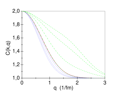
Figure 12: (color online) Same figure as the previous one, however the circulation is not the same and the displacements are equal. The dotted blue lines are for the velocity $v=0.5$ c and displacement $d_{x}=d_{z}=1.0$ fm. The dashed green lines are for the velocity $v=0.95$ c and displacement $d_{x}=d_{z}=1.0$ fm. $T_{s}=0.20$ GeV. The values of $k_{x}$ are for the blue lines: 0.5, 1.5, 3.0 and 6.0 fm^-1 and for the green lines: 0.1, 0.25, 0.5 and 1.5 fm^-1. Here the displacement is the same but the ultra-relativistic velocities lead still to the deviation in the positive direction.

By comparing Figs. 11 and 12 we see that an increase in the displacement of the sources gives a increase in the apparent size of the system (narrower $q-$distribution. We also see that the measured size of the system increases with decreasing velocity. At the same time the shape of correlation functions are becoming less and less Gaussian as the flow velocities increase. At the same time the structure of the correlation function is also very different in different directions, which is not the case for spherical or linear expansion. This indicates that the rotating system contributes to essential non-Gaussian modifications, which can be seen directly in the correlation function, but they would become invisible if we would like to fit these data with a set of Gaussians. Earlier works studied the correlation function at different angles or pseudorapidities with Gaussian parametrizations DM95 ; Sin89 , however, for rotating systems this is not the most sensitive way of presenting the results. Thus rotation can be detected even in ”symmetric” few source systems where the emission is equally probable from all emitting sources. This emission scenario is less applicable to emission from heavy ion reactions where the absorption of particles in QGP is not negligible, and this affects the emission from the interior of a timelike (spacelike) FO layer, where the emission of earlier (deeper) emitted particles are quenched.

The correlation function is symmetric in all these cases as sources from opposite sides of the system contribute equally. Thus the correlation function is not sensitive to the direction of rotation.

III Asymmetric Sources

We have seen in the previous few source model examples that a highly symmetric source may result in highly symmetric correlation functions, however, this results were not sensitive to the direction of the rotation, which seems to be unrealistic. We saw that this result is a consequence of the assumption that both of the members of a symmetric pair contribute equally to the correlation function even if one is at the side of the system facing the detector and the other is on the opposite side. The dense and hot nuclear matter or the Quark-gluon Plasma are strongly interacting, and for the most of the observed particle types the detection of a particle from the side of the system, – which is not facing the detector but points to the opposite direction, – is significantly less probable. The reason is partly in the diverging velocities during the expansion and partly to the lower emission probability from earlier (deeper) layers of the source from the external edge of the timelike (or spacelike) FO layer. This feature is recognized for a long time and discussed in detail by now. This influences the particle emission (or freeze out (FO)) process and modifies the post FO particle distribution. This topic has an extended literature, and this feature destructs the symmetry of emission of from source pairs at the opposite sides of the system Sin89 ; M-2 ; M-3 ; M-4 ; CF ; Si89 ; Bugaev ; ALM99 ; ACG99 ; MAC99 ; Cs02 ; MAA03 ; TC04 ; MCM05 ; MCM06b .

For the study of realistic systems where the emission is dominated by the side of the system, which is facing the detector, we cannot use the assumption of the symmetry among pairs or groups of the sources from opposite sides of the system. Even if the FO layer has a time-like normal direction, $\hat{\sigma}^{\mu}$ the $(k^{\mu}\hat{\sigma}^{\mu})$ factor yields a substantial emission difference between the opposite sides of the system. Now we want to demonstrate this effect on few source examples, and we will demonstrate the consequences of the non-symmetric emission.

III.1 The Emission Probability

It was first recognized that the freeze out with the Cooper-Fry description CF , may lead to negative contributions for particles, which move towards the center of the system and not in the direction out, towards the detectors. The first proposal to remedy this problem came from Bugaev Bugaev , which led to the introduction of an improved post freeze out distribution in the Cooper-Frye description, first with the Cut-Jüttner distribution Bugaev ; ACG99 and then by the Cancelling-Jüttner distribution TC04 .

Subsequently it was realized that for the realistic treatment of the freeze out process in transport theory one has to modify the Boltzmann transport equation by replacing the local molecular chaos assumption with a non-local one, where the point of origin is also included in the phase space distributions of the colliding particles. This led to the Modified Boltzmann Transport equation (MBT), and also the necessity to introduce an escape probability, $P_{esc}$ was pointed out.

The escape probability was then introduced and analysed in a series of publications M-2 ; M-3 ; M-4 ; MCM06b , in transport theoretical approaches. It was pointed out that even if the pre FO distribution is a locally equilibrated isotropic distribution, the freeze out process and the escape probability will provide a nonisotropic distribution which eliminates the earlier observed problems. This developing anisotropy in the freeze out process occurs for freeze out both in space-like and time-like directions.

The escape probability introduced in the works M-2 ; M-3 ; M-4 ; MCM06b , for a space-time surface layer of the system of thickness $L$, pointing in the four direction $\hat{\sigma}^{\mu}$ was given at a point $x^{\mu}$ inside the freeze out layer as

$$P_{esc}(x)\ \propto\ \left(\frac{L}{L-x^{\mu}\hat{\sigma}_{\mu}}\right)\left(\frac{p^{\mu}\hat{\sigma}_{\mu}}{p^{\mu}u_{\mu}}\right)\Theta(p^{\mu}\hat{\sigma}_{\mu})\,,$$ (64)

where $p^{\mu}$ is the momentum of the escaping particle, $u^{\mu}(x)$ is the local flow velocity and $s=x^{\mu}\hat{\sigma}_{\mu}$ is the distance of the emission point from the inside boundary of the layer. The first multiplicative term describes higher emission probability to the particles, which are emitted closer to the outside boundary of the layer, the second multiplicative term describes the higher emission probability for the particles, which move in the normal direction of the surface, because these should cross less material in the layer. The last term secures that only those particles can escape, which move outwards through the layer.

The last two momentum dependent factors are important in transport theoretical models, to determine the shape of the post FO momentum distribution, e.g. TC04 , which would replace the Jüttner distribution. This shape modification happens to the single and two particle distributions equally, and it acts in all emission directions, $k$, equally, so this effect is secondary from the point of view of the flow velocity dependence of the correlation function.

In order to describe the complete freeze out process for a reaction the system had to be surrounded with a freeze out layer in the space-time, and the phase space distribution of the escaping, frozen out particles can be obtained by integrating over the whole 4-volume of the freeze out layer the local (usually isotropic) phase space distribution with the escape probability $P_{esc}(x)$. This procedure would then play the role of function $G(x)$ in the source function in Eq. (10) instead of the simplified assumptions, as e.g. in Eq. (14).

The correlation function, $C(k,q)$ is always measured in a given direction of the detector, $k$. Obviously only those particles can reach the detector, which satisfy $\ k^{\mu}\hat{\sigma}_{\mu}\ >\ 0$. Thus in the calculation of $C(k,q)$ for a given $\hat{\mbox{\boldmath$k$}}$- direction we can exclude the parts of the freeze out layer where $\ k^{\mu}\hat{\sigma}_{\mu}\ <\ 0$ (see Eq. (10) of ref. Sin89 or ref. Bugaev ). For time-like FO a simplest approximation for the emission possibility is $P_{esc}(x)\ \propto\ k^{\mu}u_{\mu}(x)$ Cso-5 .

In a model calculation we therefore have to define the freeze out layer also, this realistically should not include the whole space-time volume of the reaction. In case of calculating $C(k,q)$ for a given $\hat{\mbox{\boldmath$k$}}$ we should select the relevant part of the freeze out layer, which may contribute to emission in the $k$ direction. This should be a layer of 2-3 m.f.p facing the detector at the direction $\hat{\mbox{\boldmath$k$}}$. This can eliminate the symmetric pairs of fluid cells in the previous calculations of the correlation function, even if the emission normal is timelike, because the FO particle from an earlier emission point in the ST has to propagate through the plasma for some finite time, with considerable quenching.

Therefore in the following models we should apply the escape probability and we should define a $\hat{\mbox{\boldmath$k$}}$-dependent freeze out layer also! The most simple approximation is to select an emission layer from the system for a given $\hat{\mbox{\boldmath$k$}}$-direction with uniform emission probability from within this layer. The next to most simple approximation is to introduce an emission probability within the layer, increasing towards the outside boundary of the layer. (Here it is important to mention that the spatial emission probability should be sufficiently smooth, so that one fluid cell and its contribution to $C(k,q)$, should not be effected by this emission probability.

When we have up to 4 sources we can always add $\hat{\mbox{\boldmath$k$}}$-dependent emission weights to these sources. This still would qualitatively change the outcome. As we discuss here up to four sources only a detailed formal evaluation of the emission probability would be an exaggerated approach, by defining more parameters than the outcome, so we just define the weights themselves here. In a full 3+1D fluid dynamical model with 100000+ fluid cells of course we have to apply a realistic and general evaluation of emission probability for every point of the ST.

III.2 Emission probabilities for few sources

Two sources: The previous discussion included two sources (i) in the beam-, $z-$direction and (ii) in the transverse direction in the reaction plane, $x-$direction. In case (i) the emission could be different from the two sources if the detector is in the $z-$ direction, which is difficult to achieve, so we do not have to discuss this possibility.

Figure 13: (color online) Two moving sources in the reaction ($[x-z]$) plane, separated in the $x-$ direction (case (ii) in the text). The sources are moving in the directions indicated by the (red) arrows. The detector is in the positive $x-$direction, thus the source on this side has more dominant emission into this direction, and this is indicated by the bigger size of the source on this side.

In configuration (ii) the observation can be in different $\hat{\mbox{\boldmath$k$}}$-directions. If $\hat{\mbox{\boldmath$k$}}$ points into the $\pm y-$direction, then the probabilities must be identical so emission probabilities do not lead to any change.

If $\hat{\mbox{\boldmath$k$}}$ points into the $\pm x-$direction, then one of the sources is closer to the detector and may shadow the more distant one. Thus, we can just introduce two positive weight factors so that $w_{c}$ is the weight for the cells closer to the detector and $w_{s}$ is for the cells which are far from the detector measuring the average momentum $k$. These weights are the same for the calculation of the nominator and denominator of the correlation function, so their normalization does not influence the correlation function.

As not all emitted particles reach a given detector the normalization is also dependent on the direction of the detector. Thus, we evaluate the correlation function this way. This immediately changes the earlier result (58), because it breaks the symmetry between the two sources. We can simply repeat the calculation for two moving sources in section II.2, modifying the derivation of Eq. (56) and obtain the general result

$$\begin{split}&\ \ \ \ \ \ \left.C(k,q)\!\!\phantom{\frac{1}{2}}\!\!\right|_{+x}=1+\exp(-R^{2}q^{2})\ \times\\ &\frac{w_{c}^{2}e^{\frac{2\mbox{\boldmath$k$}\mbox{\boldmath$u$}_{s}}{T_{s}}}+w_{s}^{2}e^{-\frac{2\mbox{\boldmath$k$}\mbox{\boldmath$u$}_{s}}{T_{s}}}+2w_{c}w_{s}\cosh\left(\frac{\mbox{\boldmath$q$}\mbox{\boldmath$u$}_{s}}{T_{s}}\right)\cos(2\mbox{\boldmath$q$}\mbox{\boldmath$x$}_{s})}{w_{c}^{2}e^{\frac{2\mbox{\boldmath$k$}\mbox{\boldmath$u$}_{s}}{T_{s}}}+w_{s}^{2}e^{-\frac{2\mbox{\boldmath$k$}\mbox{\boldmath$u$}_{s}}{T_{s}}}+2w_{c}w_{s}}\ .\end{split}$$ (65)

Note that this result is valid for the case when $\hat{\mbox{\boldmath$k$}}$ points to the $+x$ direction, because the weights depend on this and $w_{c}>w_{s}$. See Fig. 13. The fact that the emission from the source, which is closer to the detector is stronger makes the direction of the flow detectable.

If we introduce the notation $w_{c}=1+\epsilon$ and $w_{s}=1-\epsilon$, the deviation from the symmetric result will become apparent

$$\left.C(k,q)\!\!\phantom{\frac{1}{2}}\!\!\right|_{+x}=1+\exp(-R^{2}q^{2})\ \frac{(1+\epsilon^{2})\cosh\left(\frac{2\mbox{\boldmath$k$}\mbox{\boldmath$u$}_{s}}{T_{s}}\right)+2\epsilon\sinh\left(\frac{2\mbox{\boldmath$k$}\mbox{\boldmath$u$}_{s}}{T_{s}}\right)+(1-\epsilon^{2})\cosh\left(\frac{\mbox{\boldmath$q$}\mbox{\boldmath$u$}_{s}}{T_{s}}\right)\cos(2\mbox{\boldmath$q$}\mbox{\boldmath$x$}_{s})}{(1+\epsilon^{2})\cosh\left(\frac{2\mbox{\boldmath$k$}\mbox{\boldmath$u$}_{s}}{T_{s}}\right)+2\epsilon\sinh\left(\frac{2\mbox{\boldmath$k$}\mbox{\boldmath$u$}_{s}}{T_{s}}\right)+(1-\epsilon^{2})}\ .$$ (66)

If $\epsilon\rightarrow 0$, i.e. if $w_{c}=w_{s}$, we recover the earlier result, Eq. (57).

Figure 14: (color online) Two moving sources in the reaction ($[x-z]$) plane, separated in the $x-$ direction. The sources are moving in the directions indicated by the (red) arrows. The two ”tilted” detector directions are indicated by the (blue) arrows labeled with $k_{+}$ and $k_{-}$.

If $\epsilon=0$ we have the symmetric situation where both sources have equal contribution, the asymmetric terms vanish, and the result becomes to be symmetric for the change of the direction of the flow velocity. If $\epsilon$ reaches its maximal value, $\epsilon=1$ the contribution of the far side source is eliminated ($w_{s}=0$, $w_{c}=2$), and only the single nearby source contributes to the correlation function. In this case the asymmetric term in the nominator vanishes, the remaining terms in the nominator and denominator are equal, and we recover the single static source result.

This result has terms, which change sign if the flow velocity, ${\mbox{\boldmath$u$}}_{s}$ changes sign. The result is valid only if the detector is in the $\hat{\mbox{\boldmath$k$}}=(1,0,0)$ direction. For this direction, however, if the flow velocity points in the $z$-direction, i.e. orthogonal to $k$ the asymmetric term does not provide any contribution, so it will not show up in $C(k_{x},\mbox{\boldmath$q$})$. To circumvent this problem we should study detector directions, which do not coincide with the primary axes of the given event (where $x$ is the direction of the impact parameter vector, $b$, pointing to the projectile; $y$ is the other transverse direction; and $z$ is the direction of the projectile beam).

Figure 15: (color online) Difference of the forward and backward shifted correlation function, $\Delta C(k_{\pm},q_{out})$, for the value $\epsilon=0.50$. The solid black lines are for the velocity $v_{z}=0.5$ c, dotted blue lines are for the velocity $v_{z}=0.6$ c and dashed red lines are for the velocity $v_{z}=0.7$ c. Displacement is $d_{x}=1.0$ fm, $T_{s}=0.139$ GeV and $a=b=1/\sqrt{2}$. The values of $k$ are: for the solid black lines 0.25, 0.50, 2.00, 2.75 and 3.50 fm^-1, the dotted blue lines 0.25, 0.50, 1.00, 1.75 and 2.50 fm^-1, and the dashed red lines 0.25, 0.50, 0.75, 1.25 and 1.75 fm^-1.

Correlation in Tilted Directions: The form of the correlation function is the same if $k$ is in the same plane, the reaction plane, but it has a $z$ component also, i.e. $\mbox{\boldmath$k$}=(k_{x},0,\pm k_{z})$. This is possible for all LHC heavy ion experiments, ATLAS, CMS and even ALICE, where the longitudinal acceptance range of the TPC ($\Delta\eta\ <0.8$) is the smallest. See Fig. 14.

Earlier for spherically or longitudinally expanding systems the dependence of the correlation function on the tilt angle or width parameter was analysed in detail in ref. Sin89 . We do not go into similar fine details, just demonstrate the possibilities for an arbitrary configuration.

Depending on the detector acceptance we should chose a detector direction where $|k_{z}|$ is as big as the detector acceptance allows it. For this configuration the form of the correlation function is the same as (66)

$$\left.C(k,q)\!\!\phantom{\frac{1}{2}}\!\!\right|_{+x,\pm z}=\left.C(k,q)\!\!\phantom{\frac{1}{2}}\!\!\right|_{+x}\ ,$$ (67)

with keeping the different weights, $w_{c},w_{s}$ or $\epsilon$ so that the forward shifted and backward shifted directions have the same weights. These weights are not specified up to now anyway.

For detection of the correlation function we have to introduce here the usual, $k$-dependent coordinate system to classify the direction of $q$. Thus if

$$\hat{\mbox{\boldmath$k$}}_{\pm}=(a,0,\pm b){\rm fm}^{-1},\ k_{x}=a|\mbox{\boldmath$k$}|,\ k_{z}=\pm b|\mbox{\boldmath$k$}|,$$ (68)

where $a^{2}+b^{2}=1$, see Fig. 14. Then the difference vector, $q$, can be measured in the directions

$$\begin{split}&\hat{\mbox{\boldmath$q$}}_{out}=(a,0,\pm b),\ q_{x}=a|\mbox{\boldmath$q$}|,\ q_{z}=\pm b|\mbox{\boldmath$q$}|\\ &\hat{\mbox{\boldmath$q$}}_{side}=(0,1,0),\ \ \ q_{y}=|\mbox{\boldmath$q$}|\\ &\hat{\mbox{\boldmath$q$}}_{long}=(\mp b,0,a),\ \ q_{x}=\mp b|\mbox{\boldmath$q$}|,\ q_{z}=a|\mbox{\boldmath$q$}|.\end{split}$$ (69)

This leads to the following correlation functions

$$\begin{split}&C(k_{(\pm)},q_{out})=1+\exp(-R^{2}q^{2})\,\frac{(1{+}\epsilon^{2})\cosh\left(\frac{2\gamma k_{z}v_{z}}{T_{s}}\right)+2\epsilon\sinh\left(\frac{2\gamma k_{z}v_{z}}{T_{s}}\right)+(1{-}\epsilon^{2})\cosh\left(\frac{\gamma q_{z}v_{z}}{T_{s}}\right)\cos\left(q_{x}d_{x}\right)}{(1{+}\epsilon^{2})\cosh\left(\frac{2\gamma k_{z}v_{z}}{T_{s}}\right)+2\epsilon\sinh\left(\frac{2\gamma k_{z}v_{z}}{T_{s}}\right)+(1{-}\epsilon^{2})}\ ,\\ &C(k_{(\pm)},q_{side})=1+\exp(-R^{2}q^{2})\ ,\\ &C(k_{(\pm)},q_{long})=1+\exp(-R^{2}q^{2})\,\frac{(1{+}\epsilon^{2})\cosh\left(\frac{2\gamma k_{z}v_{z}}{T_{s}}\right)+2\epsilon\sinh\left(\frac{2\gamma k_{z}v_{z}}{T_{s}}\right)+(1{-}\epsilon^{2})\cosh\left(\frac{\gamma q_{z}v_{z}}{T_{s}}\right)\cos\left(q_{x}d_{x}\right)}{(1{+}\epsilon^{2})\cosh\left(\frac{2\gamma k_{z}v_{z}}{T_{s}}\right)+2\epsilon\sinh\left(\frac{2\gamma k_{z}v_{z}}{T_{s}}\right)+(1{-}\epsilon^{2})}\ .\end{split}$$ (70)

Although, it seems that $C(k_{(\pm)},q_{out})$ and $C(k_{(\pm)},q_{long})$ are the same, this is in fact not the case, because the values of the components of the different types of $k$ and $q$ are not the same as described in Eqs. (68,69). In all cases, the out-, side- and long- $q=|\mbox{\boldmath$q$}|$. We will also use the notation $k=|\mbox{\boldmath$k$}|$ and $\gamma v_{x}=u_{x}$, $\gamma v_{y}=u_{y}$, $\gamma v_{z}=u_{z}$, so that $\mbox{\boldmath$u$}_{s}=(u_{x},u_{y},u_{z})$. For example for the out component the difference of the forward and backward shifted correlation functions is

$$\Delta C(k_{\pm},q_{out})\equiv C(k_{+},q_{out})-C(k_{-},q_{out})=\frac{4\exp(-R^{2}q^{2})\ \epsilon\sinh\left(\frac{2u_{z}\,bk}{T_{s}}\right)\ (1{-}\epsilon^{2})\left[1-\cosh\left(\frac{u_{z}\,bq}{T_{s}}\right)\cos\left(aqd_{x}\right)\right]}{\left[(1{+}\epsilon^{2})\cosh\left(\frac{2u_{z}\,bk}{T_{s}}\right)+(1{-}\epsilon^{2})\right]^{2}-4\epsilon^{2}\sinh^{2}\left(\frac{2u_{z}\,bk}{T_{s}}\right)}.$$ (71)

As Eq. (71) and Fig. 15 show, the Differential Correlation Function (DCF), $\Delta C(k_{\pm},q_{out})$, is sensitive to the speed and direction of the rotation, and it is also sensitive to the amount of the tilt in the directions of the detection, regulated here by the parameters $a$ and $b$. $\Delta C(k_{\pm},q_{out})$ tends to zero both if $q\rightarrow 0$ and if $q\rightarrow\infty$. The structure of $\Delta C(k_{\pm},q_{out})$ is determined by the $\cosh\left(u_{z}b\,q/T_{s}\right)\,\cos\left(ad_{x}\,q\right)$ product. If in both arguments the coefficients of $q$, $u_{z}b/T_{s}$ and $ad_{x}$ are positive, smaller than one, and $u_{z}b/T_{s}\leq ad_{x}$, then the DCF is positive. If the coefficient $ad_{x}$ exceeds one the $\cos$ function changes sign at high $q_{out}$ values (e.g. above $q=1-2$fm^-1), and the DCF becomes negative at high $q_{out}$ values. Note that the ratio of the two coefficients is influenced be the choice of the tilting angle, i.e. by the parameters $a$ and $b$.

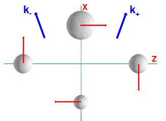
Figure 16: (color online) Four moving sources in the reaction ($[x-z]$) plane, separaed in the $x-$ and $z-$ directions. The sources are moving in the directions indicated by the (red) arrows. The ”tilted” detector directions are indicated by the (blue) arrows.

If the parameter $ad_{x}$ remains constant, about 1 fm, and then when $u_{z}b/T_{s}$ becomes larger (than one) the Differential Correlation Function becomes negative at small $q$ values.

If the parameter $u_{z}b/T_{s}$ remains constant, and about 1 fm, then when $ad_{x}$ becomes less (than one) the DCF becomes negative at small $q$ values.

In case if the detector has a narrow pseudorapidity acceptance, then $\mbox{\boldmath$k$}_{\pm}$ is close to $k_{x}$, i.e. $b\ll a$ and then the weights are maximal for the source in the $x-$direction, as indicated in Fig. 16.

If we change the direction of rotation to the opposite the Differential Correlation Function changes sign due to the $\sinh$ function in the nominator. In this configuration with the change of the tilt of the detector directions we can adjust the DCF, to the threshold value where the $\Delta C(k_{\pm},q_{out})$, is still positive, which provides a sensitive estimate for the rotation velocity at Freeze Out.

This very sensitive behaviour is rather special and it appears in this special two source model this way. With an increased resolution and with more source elements this strong and specific structure will be smoothed out to some extent.

Figure 17: (color online) Correlation function difference for the weight factors: $\omega_{a}=1.25$, $\omega_{b}=0.75$, $\omega_{c}=\omega_{d}=1.00$ for sources placed at $+x$, $-x$, $+z$ and $-z$ respectively. This weight distribution corresponds to the configuration shown in Fig. 16. The solid black lines are for the velocity $v_{z}=0.5$ c, and the dashed red lines are for the velocity $v_{z}=0.7$ c. Displacement is $d_{x}=d_{z}=1.0$ fm, $T_{s}=0.139$ GeV and $a=b=1/\sqrt{2}$. The values of $k$ are: for the solid black lines 0.10, 0.50, 1.00, and 2.00 fm^-1 and for the dashed red lines 0.10, 0.50, 1.00, and 2.00 fm^-1. The difference is larger for smaller values of $k$.

The $\sinh(2u_{z}\,bk/T_{s})$ term changes sign in the nominator when $u_{z}$ changes sign the difference of the two correlation functions, $\Delta C(k_{\pm},q_{out})$ changes sign also because all other terms are symmetric to the sign change of the velocity.

This is an important observation as we can detect the direction and magnitude of the rotation in the reaction plane. This difference is also increasing with the longitudinal shift, $b$, of the average momentum vector, $k$, so that detectors with larger pseudorapidity acceptance can detect the rotation better.

In order to perform this measurement, one has to determine the global reaction plane (e.g. from spectator residues in the ZDCs), and determine the projectile side of this plane. Furthermore the event by event center of mass should also be identified (using e.g. the method shown in ref. Eyyubova ). This will be the positive $x$-direction. Then the correlation function can be measured for four different $k$-directions in the global reaction plane. These four directions are shifted forward and backward from the center of mass symmetrically on the projectile side, and there should be a symmetric pair of detection points in the target side of the reaction plane too.

The $k$ directions opposite to each other across the c.m. point give the same result, while the difference, $\Delta C(k_{\pm},q_{out})$, between the Forward (F) and Backward (B) shifted contributions will characterize the speed and direction of the rotation. This symmetry can be used to eliminate the contribution from eventual random fluctuations. The observed F/B asymmetry depends on the parameters $\epsilon$, $v_{z}$ and $d_{x}$, these can be estimated by measuring the correlation functions at all possible moments $k$.

Fig. 15 indicates that the differential correlation function has a larger amplitude for smaller $k$ values, and the zero points are sensitively dependent on the rotation velocity.

The zero points come from the term

$$1-\cosh\left(\frac{u_{z}bq}{T_{s}}\right)\cos(aqd_{x})=0$$ (72)

Figure 18: (color online) Correlation function difference for the weight factors: $\omega_{a}=1.25$, $\omega_{b}=0.75$, $\omega_{c}=\omega_{d}=1.00$ for sources placed at $+x$, $-x$, $+z$ and $-z$ respectively. This weight distribution corresponds to the configuration shown in Fig. 16. The solid black lines are for the velocity $v_{z}=0.5$ c, and the dashed red lines are for the velocity $v_{z}=0.7$ c. Displacement is $d_{x}=d_{z}=1.0$ fm, $T_{s}=0.139$ GeV and $a=4b=4/\sqrt{17}$. The values of $k$ are: for the solid black lines 0.10, 1.00, 3.00, and 5.00 fm^-1 and for the dashed red lines 0.10, 1.00, 3.00, and 5.00 fm^-1. For a detector with narrow pseudorapidity acceptance we could use a value $a>b$. For this figure we have used $a=4b$. We can compare this with Fig. 17, and we see that for $q>1.5$ fm^-1 they are very similar. The DCF has a smaller amplitude in the positive direction for values around $q<1.0$ fm^-1, but a larger amplitude in the negative direction for values around $0.75$ fm${}^{-1}\,<q<1.5$ fm^-1. We also see that the DCF is not close to zero for values around $2.0$ fm${}^{-1}<k<5.0$ fm^-1.

and it is not dependent on $k$, so for the values used in Fig. 15 and $q=x\,$fm^-1 we have

$$\cosh\left(\frac{0.197}{0.139}\frac{v_{z}/c}{\sqrt{1-v^{2}_{z}/c^{2}}}\frac{x}{\sqrt{2}}\right)\cos\left(\frac{x}{\sqrt{2}}\right)=1\ .$$ (73)

Since the cosine term must be positive, there are no zero points for $\pi/\sqrt{2}\leq x\leq 3\pi/\sqrt{2}$ or $2.23\leq x\leq 6.66$.

For $x>3\pi/\sqrt{2}$ the $\exp(-R^{2}x^{2})$ term will be small and there would be no correlation difference. So we will look at the values $0<x<\pi/\sqrt{2}$

If $v_{z}$ is smaller than $0.57c$ then there will be no zero point for $0<x<\pi/\sqrt{2}$. For $v_{z}$ larger than $0.58c$ there will be 1 zero point for $0<x<\pi/\sqrt{2}$.

The zero point for a given velocity can be found by solving equation (73) numerically. For velocities $v=0.6c$ and $v=0.7c$ we have zero points at $q=0.83\,fm^{-1}$ and $q=1.69\,fm^{-1}$ respectively.

This indicates the sensitivity of the method and the possibility to influence it by the choice of the detector directions (via the choice of $a$ and $b$).

III.3 Emission from four sources

With four sources we can illustrate the possibilities of differential HBT method studies in different directions. The correlation functions can be calculated in general for four sources and two detector positions. This can then be applied to different detector configurations.

The out component of the four source correlation function with weight factors $\omega_{a}$, $\omega_{b}$, $\omega_{c}$, $\omega_{d}$ is given by

$$\begin{split}&C(k_{(\pm)},q_{out})=1+\exp(-R^{2}q^{2})\,\left[2\omega_{a}\omega_{b}+2\omega_{c}\omega_{d}+\right.\\ &\left.\omega_{a}^{2}\exp\left(\pm\frac{2\gamma v_{z}bk}{T_{s}}\right)\exp\left(\pm\frac{\gamma v_{z}bq}{T_{s}}\right)\cos(2ad_{x}q)+\omega_{b}^{2}\exp\left(\mp\frac{2\gamma v_{z}bk}{T_{s}}\right)\exp\left(\mp\frac{\gamma v_{z}bq}{T_{s}}\right)\cos(2ad_{x}q)+\right.\\ &\left.\omega_{c}^{2}\exp\left(\frac{2\gamma v_{x}ak}{T_{s}}\right)\exp\left(\frac{\gamma v_{x}aq}{T_{s}}\right)\cos(2bd_{z}q)+\omega_{d}^{2}\exp\left(-\frac{2\gamma v_{x}ak}{T_{s}}\right)\exp\left(-\frac{\gamma v_{x}aq}{T_{s}}\right)\cos(2bd_{z}q)+\right.\\ &\left.2\omega_{a}\omega_{c}\exp\left(\pm\frac{\gamma v_{z}bk}{T_{s}}\right)\exp\left(\pm\frac{\gamma v_{z}bq}{2T_{s}}\right)\exp\left(\frac{\gamma v_{x}ak}{T_{s}}\right)\exp\left(\frac{\gamma v_{x}aq}{2T_{s}}\right)\cos((ad_{x}\pm bd_{z})q)+\right.\\ &\left.2\omega_{b}\omega_{d}\exp\left(\mp\frac{\gamma v_{z}bk}{T_{s}}\right)\exp\left(\mp\frac{\gamma v_{z}bq}{2T_{s}}\right)\exp\left(-\frac{\gamma v_{x}ak}{T_{s}}\right)\exp\left(-\frac{\gamma v_{x}aq}{2T_{s}}\right)\cos((ad_{x}\pm bd_{z})q)+\right.\\ &\left.2\omega_{a}\omega_{d}\exp\left(\pm\frac{\gamma v_{z}bk}{T_{s}}\right)\exp\left(\pm\frac{\gamma v_{z}bq}{2T_{s}}\right)\exp\left(-\frac{\gamma v_{x}ak}{T_{s}}\right)\exp\left(-\frac{\gamma v_{x}aq}{2T_{s}}\right)\cos((ad_{x}\mp bd_{z})q)+\right.\\ &\left.2\omega_{b}\omega_{c}\exp\left(\mp\frac{\gamma v_{z}bk}{T_{s}}\right)\exp\left(\mp\frac{\gamma v_{z}bq}{2T_{s}}\right)\exp\left(\frac{\gamma v_{x}ak}{T_{s}}\right)\exp\left(\frac{\gamma v_{x}aq}{2T_{s}}\right)\cos((ad_{x}\mp bd_{z})q)\right]\times\\ &\left[\omega_{a}\exp\left(\pm\frac{\gamma v_{z}bk}{T_{s}}\right)+\omega_{b}\exp\left(\mp\frac{\gamma v_{z}bk}{T_{s}}\right)+\omega_{c}\exp\left(\frac{\gamma v_{x}ak}{T_{s}}\right)+\omega_{d}\exp\left(-\frac{\gamma v_{x}ak}{T_{s}}\right)\right]^{-2}\ .\end{split}$$ (74)

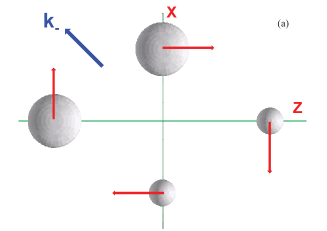
Figure 19: (color online) Four moving sources in the reaction ($[x-z]$) plane, separated in the $x-$ and $z-$ directions. The sources are moving in the directions indicated by the (red) arrows. The ”tilted” detector directions are indicated by the (blue) arrows. In the two configurations, (a) and (b) the detector directions are different and the weights of the sources are also different, so that the sources closer to the detector direction have larger weights.

Two examples on different detector configurations are given in Figs. 16 and 19. We use the same equations as in the two source model, Eqs. (68) and (69).

A source with a larger weight factor is closer to the detector, so that $\omega_{a}$, $\omega_{b}$, $\omega_{c}$, $\omega_{d}$ correspond to $\mbox{\boldmath$x$}_{s}\equiv(r_{x},r_{z})=(d_{x},0),(-d_{x},0),(0,d_{z}),(0,-d_{z})$ respectively.

In case if the detector has a wide pseudorapidity acceptance, then $\mbox{\boldmath$k$}_{\pm}$ can deviate significantly from $k_{x}$, i.e. $b\geq a$ and then the weights are maximal for the two sources closest to $\mbox{\boldmath$k$}_{+}$ or $\mbox{\boldmath$k$}_{-}$ as indicated in Fig. 19.

Eq. (74) can be used to find the difference of the forward and backward shifted correlation function. We will use that $d_{x}=d_{z}$, $v_{x}=v_{z}$ and $a=b$.

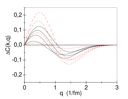
Figure 20: (color online) Correlation function difference for the weight factors: $\omega_{a}=1.25$, $\omega_{b}=0.75$, $\omega_{c}=0.50$, $\omega_{d}=1.50$ for sources placed at $+x$, $-x$, $+z$ and $-z$ respectively (Fig. 19a) and $\omega_{a}=1.25$, $\omega_{b}=0.75$, $\omega_{c}=1.50$, $\omega_{d}=0.50$ for sources placed at $+x$, $-x$, $+z$ and $-z$ respectively (Fig. 19b). The solid black lines are for the velocity $v_{z}=0.5$ c, and the dashed red lines are for the velocity $v_{z}=0.7$ c. Displacements are $d_{x}=d_{z}=1.0$ fm, $T_{s}=0.139$ GeV and $a=b=1/\sqrt{2}$. The values of $k$ for both series of lines are 0.10, 0.50, 1.00, and 2.00 fm^-1. The difference is larger for smaller values of $k$.

Some examples for the differential correlation functions are shown in Figs. 17 and 20. Here due to the simplified few source model we specified the weight distribution among the sources in a simplified way. For realistic high resolution fluid dynamical model calculatios the realistic evaluation of emission probabilities is necessary.

We can compare Fig. 17 with the previously shown two source model, Fig. 15, and we see that the amplitudes are similar but the shapes are different. First of all the sensitivity on the direction of rotation remained the same as in the simpler two source model. The two extra sources, $c$ and $d$ lead to higher amplitude for the Differential Correlation Function, while the regular positions of the locations of the zero points are varying due to more sources with different weight parameters.

In Fig. 18 we show the DCF for a configuration where the deviation between $\mbox{\boldmath$k$}_{+}$ and $\mbox{\boldmath$k$}_{-}$ is smaller, like shown in Fig. 16. This configuration can be applied in detectors where the pseudorapidity acceptance range of the detector is not wide. Still the rotation is well detectable. In this configuration the accurate determination of the reaction plane and the participant center of mass momentum is more important.

If the detector acceptance is wider, then the two detectors can be placed at more different angles. This configuration makes the forward and backward placed sources more accessible to the forward and backward detectors, respectively. This is taken into account in the emission weights of our sources. These weights are now different for the two components of the DCF!

The result shows the tendency that the DCF has a similar structure in the two source model and the four source model in a resembling configuration. Fig. 20 has the same shape as Fig. 17, but the amplitude is larger.

For a set of large number of sources, forming a system with close to perfect rotational symmetry, a single correlation function would not depend on the (polar) angle of the detection, and the DCF would vanish. Thus, the DHBT method would not be applicable for highly symmetric systems, like for a rotating star observed from within the plane of the rotation. At the same time for a rotating binary star system the DHBT method would work. Also the weighting of the sources should be different: If the observer is in the plane of rotation, the distant star is shadowed by the front one at some periods, just like emission from a highly opaque plasma (evidenced by jet quenching). If the observer is slightly out of the plane of rotation then the two stars are visible all the time and then the (time dependent) correlation function would change between the configurations of Figs. 4 and 7. This also illustrates the role of symmetric and asymmetric weightings.

The rotating and expanding final state of a relativistic heavy ion reaction is of course does not look like a perfect wheel, so the four source model is a more adequate approximation than a wheel would be.

IV Conclusions

In this work we attempted to study the possibility of detecting and evaluation the rotation of a source by the specific use of the Hanbury-Brown and Twiss method for rotating systems. Our primary interest was the application for ultra-relativistic heavy ins where in peripheral collisions at ultra-relativistic energies the system can gain large angular momentum. Nevertheless, some of the conclusions can be applied to macroscopic systems also, like for past rotating stars.

We selected one of the several methods to evaluate two particle correlations, which was suitable to study collective fluid systems with significant and well defined internal fluid dynamical motion. The obtained standard correlation functions were showing the consequences of the flow, but for highly symmetric sources the correlation functions gave symmetric results, which were invariant for the change of the direction of rotation.

It turned out that it is important to take into account that the particles reaching the detector cannot reach it with equal probability from the near side and the far side of the emitting object. With this fact considered we could obtain correlation functions, which reflected the properties and also the direction of the flow. These results can be used rather generally.

The obtained results have shown that the correlation function is most sensitive to the rotation if it is measured in the beam direction (or close to it). This, unfortunately, is not possible in most heavy ion accelerator experiments, so we introduced and investigated a Differential Hanbury Brown and Twiss method, which made it possible to trace down the rotation in relativistic heavy ion collisions by measuring the correlation functions in the reaction plane at nearly transverse angles to the beam direction. The method is promising and can be performed in most heavy ion experiments without difficulties, as well as it can be implemented in different reaction models, like fluid dynamical models, microscopic transport models and hybrid models. In full scale theoretical models, the emission probabilities from the FO layer have to be considered. From the general formulas derived in the beginning of the paper apparently these dependencies can be factorized.

To complement these studies we also applied the method to a high resolution, 3+1D, computational fluid dynamics model CVW2013 , which was used earlier to predict roation, KHI, flow vorticity, and polarization hydro1 ; hydro2 ; CMW12 ; BCW2013 . The result shows that the method can detect rotation, while the effects of irregular shape, sperical flow, and specific flow patterns, require a more extended analysis to separate all these effects form one another.

- (1) L.P. Csernai, V.K. Magas, H. Stöcker, and D.D. Strottman, Phys. Rev. C 84, 024914 (2011).
- (2) L.P. Csernai, D.D. Strottman and Cs. Anderlik, Phys. Rev. C 85, 054901 (2012).
- (3) D.J. Wang, Z. Néda, and L.P. Csernai Phys. Rev. C 87, 024908 (2013). arXiv: 1302.1691v1 [nucl-th].
- (4) L.P. Csernai, V.K. Magas, and D.J. Wang, Phys. Rev. C 87, 034906 (2013).
- (5) R. Hanbury Brown and R.Q. Twiss, Phil. Mag. 45, 663 (1954); and R. Hanbury Brown and R.Q. Twiss, Nature, 178, 1046 (1956).
- (6) G. Goldhaber, S. Goldhaber, W. Lee and A. Pais, Phys. Rev. 120, 300 (1960).
- (7) D. Miskowiec, and E877 Collaboration, Nucl. Phys. A 590, 557c (1995).
- (8) M.A. Lisa, N.N. Ajitanand, J.M. Alexander, et al., Phys. Lett. B 496, 1 (2000); M.A. Lisa, U. Heinz, U.A. Wiedemann, Phys. Lett. B 489, 287 (2000); E. Mount, G. Graef, M. Mitrovski, M. Bleicher, M.A. Lisa, Phys. Rev. C 84, 014908 (2011).
- (9) S. Pratt, Phys. Rev. D 33, 1314 (1986);
- (10) Yu.M. Sinyukov, Nucl. Phys. A498 (1989) 151c.
- (11) Qingfeng Li, J. Steinheimer, H. Petersen, M. Bleicher, H. Stöcker, Phys. Lett. B 674, 111 (2009); Qingfeng Li, M. Bleicher, H. Stöcker, Phys. Lett. B 659 525 (2008); Qingfeng Li, M. Bleicher, Xianglei Zhu, H. Stöecker, J. Phys. G 33 537 (2007).
- (12) M.A. Lisa, S. Pratt, R. Soltz, U. Wiedemann, Annual Review of Nuclear and Particle Science, 55, 357 (2005).
- (13) L.P. Csernai: Introduction to relativistic heavy ion collisions, Wiley, Chichester (1994).
- (14) F. Cooper, G. Frye, Phys. Rev. D 10, 186 (1974).
- (15) W. Florkowski: Phenomenology of Ultra-relativistic heavy-Ion Collisions, World Scientific Publishing Co., Singapore (2010).
- (16) Cheuk-Yin Wong: Introduction to heavy ion reactions, World Scientific Publishing Co., Singapore (1994)
- (17) E. Molnár, L. P. Csernai, V. K. Magas, Zs. I. Lazar, A. Nyiri, and K. Tamosiunas, J. Phys. G 34, 1901 (2007).
- (18) E. Molnár, L. P. Csernai, V. K. Magas, A. Nyiri, and K. Tamosiunas, Phys. Rev. C 74, 024907 (2006).
- (19) E. Molnár, L.P. Csernai, V.K. Magas, Acta Phys. Hung. A 27, 359 (2006); arXiv: nucl-th/0510062.
- (20) T. Csörgő, Heavy Ion Phys. 15, 1-80, (2002); arXiv: hep-ph/0001233v3.
- (21) D. Anchishkin, V. Vovchenko, L.P. Csernai, Phys. Rev. C 87, 014906 (2013).
- (22) A.N. Makhlin, Yu.M. Sinyukov, Z. Phys. C 39, 69-73 (1988).
- (23) I.S. Gradshteyn and I.M. Ryzhik: Table of integrals, series and products, Academic Press (1965).
- (24) Sz. Horvát, V.K. Magas, D.D. Strottman, L.P. Csernai, Phys. Lett. B 692, 277 (2010).
- (25) P.K. Kovtun, D.T. Son and A.O. Starinets, Phys. Rev. Lett. 94, 111601 (2005).
- (26) L.P. Csernai, J.I. Kapusta, L.D. McLerran, Phys. Rev. Lett. 97, 152303–4 (2006).
- (27) L.P. Csernai, G. Eyyubova, V.K. Magas, Phys. Rev. C 86, 024912 (2012).
- (28) Stefan Floerchinger and Urs Achim Wiedemann, Journal of High Energy Physics, JHEP 11, 100 (2011); and J. Phys. G: Nucl. Part. Phys. 38, 124171 (2011).
- (29) Yu.M. Sinyukov, Yad. Fiz. 50, 228 (1989); Sov. J. Nucl. Phys. 50, 143 (1989); Z. Phys. C 43, 401 (1989).
- (30) K.A. Bugaev, Nucl. Phys. A 606, 559 (1996).
- (31) Cs. Anderlik, Z.I. Lázár, V.K. Magas, L.P. Csernai, H. Stöcker and W. Greiner, Phys. Rev. C 59, 388 (1999).
- (32) C. Anderlik, L.P. Csernai, F. Grassi, W. Greiner, Y. Hama, T. Kodama, Z.I. Lázár, V.K. Magas and H. Stöcker, Phys. Rev. C 59, 3309 (1999) .
- (33) V.K. Magas, C. Anderlik, L.P. Csernai, F. Grassi, W. Greiner, Y. Hama, T. Kodama, Z.I. Lázár and H. Stöcker, Nucl. Phys. A 661, 596c (1999).
- (34) L.P. Csernai, J. Phys. G 28, 1993 (2002).
- (35) V.K. Magas, A. Anderlik, Cs. Anderlik and L.P. Csernai, Eur. Phys. J. C 30, 255 (2003).
- (36) K. Tamosiunas and L.P. Csernai, Eur. Phys. J. A 20, 269 (2004).
- (37) V.K. Magas, L.P. Csernai, E. Molnár, A. Nyiri and K. Tamosiunas, Nucl. Phys. A 749, 202 (2005).
- (38) V.K. Magas, L.P. Csernai, E. Molnár, Acta Phys. Hung. A 27, 351 (2006); arXiv: nucl-th/0510066.
- (39) L.P. Csernai, S. Velle, D.J. Wang, (2013) arXiv:1305.0396
- (40) F. Becattini, L.P. Csernai, D.J. Wang, arXiv:1304.4427v1 [nucl-th]