Gaussian Quadrature and Lattice Discretization of the
Fermi-Dirac Distribution for Graphene

Abstract

We construct a lattice kinetic scheme to study electronic flow in graphene. For this purpose, we first derive a basis of orthogonal polynomials, using as weight function the ultrarelativistic Fermi-Dirac distribution at rest. Later, we use these polynomials to expand the respective distribution in a moving frame, for both cases, undoped and doped graphene. In order to discretize the Boltzmann equation and make feasible the numerical implementation, we reduce the number of discrete points in momentum space to $18$ by applying a Gaussian quadrature, finding that the family of representative wave (2+1)-vectors, that satisfies the quadrature, reconstructs a honeycomb lattice. The procedure and discrete model are validated by solving the Riemann problem, finding excellent agreement with other numerical models. In addition, we have extended the Riemann problem to the case of different dopings, finding that by increasing the chemical potential, the electronic fluid behaves as if it increases its effective viscosity.

I Introduction

Since its discovery Novoselov et al. (2005, 2004), graphene has shown a series of wonderful electrical and mechanical properties, such as ultra-high electrical conductivity, ultra-low viscosity, as well as exceptional structural strength, combined with mechanical flexibility and optical transparence. Due to the special symmetries of the honeycomb lattice, electrons in graphene are shown to behave like massless chiral ultrarelativistic quasiparticles, propagating at a Fermi speed of about $v_{F}\sim 10^{6}$ m/s DiVincenzo and Mele (1984); Das Sarma et al. (2011). This places graphene as an appropriate laboratory for experiments involving relativistic massless particles confined to a two-dimensional space Geim and MacDonald (2007).

Electronic gas in graphene can be approached from a hydrodynamic perspective Müller et al. (2009); Müller and Sachdev (2008); Fritz et al. (2008); Müller et al. (2008), behaving as a nearly perfect fluid reaching viscosities significantly smaller than those of superfluid Helium at the lambda-point. This has suggested the possibility of observing pre-turbulent regimes, as explicitly pointed out in Ref. Müller et al. (2009) and later confirmed by numerical simulations Mendoza et al. (2011). All these characteristics in graphene open up the possibility of studying several phenomena known from classical fluid dynamics, e.g. transport through disordered media Mendoza et al. (2013a), Kelvin-Helmholtz and Rayleigh Bénard instabilities, just to name a few. However, the study of these phenomena needs appropriate numerical tools, which take into account both, the relativistic effects and the Fermi-Dirac statistics.

Recently, a solver for relativistic fluid dynamics based on a minimal form of the relativistic Boltzmann equation, whose dynamics takes place in a fully discrete phase-space lattice and time, known as relativistic lattice Boltzmann (RLB), has been proposed by Mendoza et al. Mendoza et al. (2010a, b) (and subsequently revised in Ref. Hupp et al. (2011) enhancing numerical stability). This model reproduces correctly shock waves in quark-gluon plasmas, showing excellent agreement with the solution of the full Boltzmann equation obtained by Bouras et al. using BAMPS (Boltzmann Approach Multi-Parton Scattering) Xu and Greiner (2005); Bouras et al. (2009). In order to set up a theoretical background for the lattice version of the relativistic Boltzmann equation for the Boltzmann statistics, Romatschke et al. Romatschke et al. (2011) developed a scheme for an ultrarelativistic gas based on the expansion in orthogonal polynomials of the Maxwell-Jüttner distribution Cercignani and Kremer (2002) and, by following a Gauss-type quadrature procedure, the discrete version of the distribution and the weight functions was calculated. This procedure was similar to the one used for the non-relativistic lattice Boltzmann model He and Luo (1997a); Martys et al. (1998); He and Luo (1997b); Succi (2001). This relativistic model showed very good agreement with theoretical data, although it was not compatible with a lattice, thereby requiring linear interpolation in the free-streaming step. Another model based on a quadrature procedure was developed recently in order to make the relativistic lattice Boltzmann model compatible with a lattice Mendoza et al. (2013b). However, all these models are based on the the Maxwell-Jüttner distribution, which is based on the Boltzmann statistics, and therefore, their applications to quantum systems is limited.

In this work, we construct a family of orthogonal polynomials by using the Gram-Schmidt procedure using as weight function the ultrarelativistic Fermi-Dirac distribution at rest. By applying a Gauss-type quadrature, we find that the family of discrete (2+1)-momentum vectors, needed to recover the first three moments of the equilibrium distribution, are fully compatible with a hexagonal lattice, avoiding any type of linear interpolation. This result is very convenient, since the crystal of graphene shares the same geometry, facilitating the implementation of boundary conditions, allowing for instance having a good approximation for the electronic transport in nanoribbons with armchair or zigzag edges Han et al. (2007); Barone et al. (2006) by implementing the typical bounce-back rule for lattice Boltzmann models.

The paper is organized as follows: in Sec. II, we describe in details the expansion of the Fermi-Dirac distribution in an orthogonal basis of polynomials, and perform the Gauss-type quadrature. In this section, we also explain the discretization procedure. In Sec. III, we implement the validation of our model by simulating the Riemann problem; and in Sec. IV, we perform additional simulations for doped graphene. Finally, in Sec. V, we discuss the results and future work.

II Model Description

The electronic gas in graphene can be considered as a gas of massless Dirac quasi-particles obeying the Fermi-Dirac statistics in a two-dimensional space. Thus, we define the single-particle distribution function $f(x^{\mu},p^{\mu})$ in phase space, being $x^{\mu}=(x^{0},x^{1},x^{2})$ and $p^{\mu}=(p^{0},p^{1},p^{2})$ the time-position and energy-momentum coordinates, respectively. Here $x^{0}$ denotes time, $\vec{x}=(x^{1},x^{2})$ spatial coordinates, $p^{0}$ the energy, and $\vec{p}=(p^{1},p^{2})$ the momentum of the particles. In the ultrarelativistic regime, we get $p^{\mu}p_{\mu}=0$ (in this paper we use the Einstein notation, i.e. repeated indexes denote summing over such indexes). In our approach, we assume that the distribution function $f$ evolves according to the relativistic Boltzmann-BGK equation Cercignani and Kremer (2002),

$$p^{\mu}\partial_{\mu}f=-\frac{p_{\alpha}U^{\alpha}}{v_{F}^{2}\tau}(f-f_{eq})\quad,$$ (1)

where $\tau$ is the relaxation time, and $f_{eq}$ the equilibrium distribution, which in our case, is the relativistic Fermi-Dirac distribution defined by

$$f_{eq}(x^{\mu},p^{\mu})=\frac{1}{\text{e}^{(p_{\alpha}U^{\alpha}-\mu)/k_{B}T}+1}\quad,$$ (2)

with $T$ the temperature, $k_{B}$ the Boltzmann constant, $U^{\mu}$ the macroscopic (2+1)-velocity of the fluid Jüttner (1928); Cercignani and Kremer (2002), and $\mu$ the chemical potential. The relation between the Lorentz-invariant $U^{\mu}$ and the classical velocity $\vec{u}=(u^{1},u^{2})$ is given by $U^{\mu}=\gamma(v_{F},u^{1},u^{2})$, with $v_{F}$ being the Fermi speed and $\gamma=1/\sqrt{1-\vec{u}^{2}/v_{F}^{2}}$.

II.1 Moment expansion

Here, we perform an expansion of the Fermi-Dirac distribution, Eq. (2), in an orthogonal basis of polynomials. In our case, since we are interested in the hydrodynamic regime, we will truncate the expansion preserving only the polynomials up to second order, although achieving higher orders is also possible by using the same procedure. In particular, we need to reproduce the first three moments of the equilibrium Fermi-Dirac distribution, namely $\langle 1\rangle_{(eq)}$, $\langle p^{\alpha}\rangle_{(eq)}$, and $\langle p^{\alpha}p^{\beta}\rangle_{(eq)}$ for $\alpha,\beta=0,1,2$. The angular brackets denote expectation values using the distribution $f$ via $\langle Q\rangle=\int\text{d}\mu\,Qf$, with $\text{d}\mu=d^{2}p/2p^{0}(2\pi)^{2}$, and the subscript _(eq) indicates that the equilibrium distribution $f_{eq}$ is taken instead of $f$.

This method was originally introduced by Grad Grad (1949) who expanded the Maxwell-Boltzmann distribution in Hermite polynomials, based on the fact that they are orthogonal, using as weight function the Maxwellian distribution at rest. In this spirit, we will derive a new basis of polynomials that are orthogonal with respect to the Fermi-Dirac distribution at rest,

$$w(p_{0})=\frac{1}{\text{e}^{p_{0}/k_{B}T}+1}\quad.$$ (3)

For the following derivations it is useful to choose natural units, $c=k_{B}=\hbar=1$. In addition, we will consider only the case for $\mu=0$, although a general approach is straightforward. By introducing a reference temperature $T_{0}$, we define $\theta=T/T_{0}$, $\bar{p}=p^{0}/T_{0}$, $\vec{v}=\vec{p}/|\vec{p}|$, and using $p^{0}=|\vec{p}|$, we rewrite the equilibrium distribution as

$$f_{eq,E}(t,\vec{x},\bar{p},\vec{v})=\frac{1}{\text{e}^{\bar{p}\gamma(1-\vec{v}\cdot\vec{u})/\theta}+1}\quad,$$ (4)

where the subscript $E$ stands for “Exact”. The distribution $f_{eq,E}$ is expanded using tensorial polynomials $P^{(n)}$, for the angular contribution, and $F^{(k)}$, for the radial dependence, such that

$$f_{eq,E}(t,\vec{x},p,\vec{v})=\frac{1}{\text{e}^{\bar{p}}+1}\sum_{n,k}^{\infty}a^{(nk)}_{\underline{i}}(t,\vec{x})P^{(n)}_{\underline{i}}(\vec{v})F^{(k)}(\bar{p})\quad.$$ (5)

Here, the (2+1)-momentum vectors have been expressed in polar coordinates, $p^{\mu}=(\bar{p},\bar{p}\cos\phi,\bar{p}\sin\phi)$ with $\vec{v}=(\cos\phi,\sin\phi)$ being a unit vector that carries the angular dependence $\phi$, and the index $\underline{i}$ denotes a family of indices $i_{1},...,i_{n}\in\{1,2\}$ whose total number equals the order $n$ of the tensor for the angular dependence, i.e. $P^{(n)}_{\underline{i}}$ and $a^{(nk)}_{\underline{i}}$ are tensors of rank $n$. Such an ansatz has been used by Romatschke et al. Romatschke et al. (2011) to expand the Maxwell-Jüttner distribution. Employing the Gram-Schmidt procedure, the radial polynomials $F^{(k)}$ are constructed satisfying the orthogonality relation

$$\int_{0}^{\infty}\frac{\text{d}\bar{p}}{4\pi}w(\bar{p})F^{(k)}(\bar{p})F^{(l)}(\bar{p})=\Gamma^{(k)}_{F}\delta_{kl}\quad,$$ (6)

and the angular ones by satisfying

$$\int_{0}^{2\pi}\frac{\text{d}\phi}{2\pi}P^{m}_{\underline{i}}(\phi)P^{n}_{\underline{j}}(\phi)=\Gamma^{(m)}_{P,\underline{i}\underline{j}}\delta_{mn}\quad.$$ (7)

The resulting polynomials and $\Gamma$-constants up to second order are given in Appendix  A. With these polynomials and taking into account Eq. (5), one can show that up to second order in $n$ and $k$, we get

$$a^{(nk)}_{\underline{i}}=\frac{g^{(n)}}{\Gamma_{F}^{(k)}}T_{0}\int\frac{\text{d}\bar{p}}{4\pi}\frac{\text{d}\phi}{2\pi}f_{eq,E}P^{(n)}_{\underline{i}}F^{(k)}\quad,$$ (8)

with $g^{(0)}=1$, $g^{(1)}=2$, and $g^{(2)}=4$. The explicit form of $a^{(nk)}$ is given in Appendix B. Using Eq. (5), the definitions of the polynomials, and their orthogonality relations it can be easily shown that the moments up to second order can be written in terms of the coefficients $a^{(nk)}_{\underline{i}}$ with $n,k\leq 2$ (see Appendix B), and therefore, the truncated expansion of the distribution $f_{eq}$ up to second order becomes

$$f_{eq}=\frac{1}{\text{e}^{\bar{p}}+1}\sum_{n=0}^{2}\sum_{k=0}^{2}a^{(nk)}_{\underline{i}}P^{(n)}_{\underline{i}}F^{(k)}\quad.$$ (9)

This is sufficient to recover the moments

$$\langle p^{\alpha}\rangle_{(eq)}=nU^{\alpha}\quad,$$ (10a)

$$\langle p^{\alpha}p^{\beta}\rangle_{(eq)}=(\epsilon+P)U^{\alpha}U^{\beta}-P\eta^{\alpha\beta}\quad,$$ (10b)

of the full Fermi-Dirac distribution, Eq. (4). In Eq. (10b), we have introduced the Minkowski metric tensor $\eta^{\alpha\beta}$, the particle density $n=\frac{\pi}{48}T^{2}$, the pressure $P=\frac{9\zeta(3)}{\pi^{2}}nT$ and the energy density $\epsilon=2P$, where $\zeta$ denotes the Riemann zeta function, $\zeta(3)\approx 1.202$.

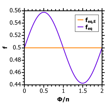
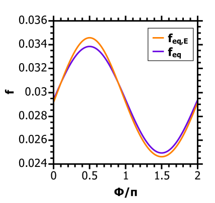
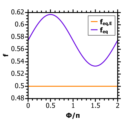
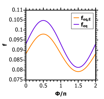
Figure 1: Comparison betweem the expanded Fermi dirac distribution $f_{eq}$ and the full version $f_{eq,E}$ as a function of the angular component $\phi$, for $\bar{p}=0$ (left) and $\bar{p}=3.5$ (right), with $\theta=1.0$ (top) and $\theta=1.5$ (bottom), $u^{1}=0.0$, $u^{2}=0.05$.

Fig. 1 shows that the quality of the matching between the truncated $f_{eq}$ and the exact $f_{eq,E}$, for $\bar{p}\sim 0$, is very poor, in contrast with the case, $\bar{p}\sim 3.5$. However, this is not surprising, since we are dealing with a gas of ultrarelativistic particles which are always moving at the Fermi speed, and therefore none of them has energy $\bar{p}=0$. On the other hand, the matching is reasonable for $\theta=1$, while being off for $\theta>1$. Thus, we conclude that $\theta=1$ offers the best approximation, and therefore, we will work with that value. In addition, we have found that $\theta$ cannot be chosen far below unity because $f_{eq}$ can present negative values. The fact that $\theta=1$ implies that the reference temperature $T_{0}$ should be equal to the temperature of the electronic gas $T$.

II.2 Momentum space discretization

We now need to discretize the momentum space into a finite number $N$ of discrete momentum vectors, $p^{\mu}_{q}$ (with $q=0,...,N$) such that we can replace integrals in the continuum momentum space by sums over a small number of discrete momentum (2+1)-vectors. In order to do that, we use the Gaussian quadrature Davis and Rabinowitz (1984). As an example, for the radial dependence of the expansion, in order to satisfy

$$\int_{0}^{\infty}\frac{\text{d}\bar{p}}{4\pi}w(\bar{p})F^{(k)}(\bar{p})\bar{p}^{l}=\sum_{q^{\prime}=0}^{N}\frac{\omega^{(\bar{p})}_{q^{\prime}}}{w(\bar{p}_{q^{\prime}})}w(\bar{p}_{q^{\prime}})F^{(k)}(\bar{p}_{q^{\prime}})\bar{p}^{l}_{q^{\prime}}\quad,$$ (11)

for $k,l\leq 2$, we should calculate the discrete $\bar{p}_{q^{\prime}}$ and respective radial weights $\omega^{(\bar{p})}_{q^{\prime}}$. By using the Gaussian quadrature theorem, we found the following values:

$$\bar{p}_{1}=0.484, ~{}\omega^{(\bar{p})}_{1}=0.0369$$

$$\bar{p}_{2}=2.447, ~{}\omega^{(\bar{p})}_{2}=0.0176$$

$$\bar{p}_{3}=6.424, ~{}\omega^{(\bar{p})}_{3}=0.000719\quad.$$

Note that in fact, $\bar{p}$ is always larger than zero, as expected for ultrarelativistic particles, (see Appendix C for numerical values with higher precision).

On the other hand, by following a similar procedure, we can calculate the $N^{\prime}$ discrete angles $\phi_{q^{\prime\prime}}$ and angular weights $\omega^{(\phi)}_{q^{\prime\prime}}$ (with $q^{\prime\prime}=1,...,N^{\prime}$), such that, for the angular integrals over $P^{(n)}(v_{i})^{l}(v_{j})^{m}$, one gets

$$\int_{0}^{2\pi}\frac{\text{d}\phi}{2\pi}P^{(n)}(v_{i})^{l}(v_{j})^{m}=\sum_{q^{\prime\prime}=0}^{N^{\prime}}\omega^{(\phi)}_{q^{\prime\prime}}P^{(n)}(v_{i,q^{\prime\prime}})^{l}(v_{j,q^{\prime\prime}})^{m}\quad,$$ (12)

where $v_{i,q^{\prime\prime}}$ denotes $v_{i}(q^{\prime\prime})$. The above expression is required to be an exact quadrature formula for $n\leq 2$, and $l+m\leq 2$. The results for the discrete angles and weights functions are $\phi_{q^{\prime\prime}}=\frac{\pi}{2}+(q^{\prime\prime}-1)\frac{\pi}{3}$ and $\omega^{(\phi)}_{q^{\prime\prime}}=\frac{1}{6}$ with $N^{\prime}=6$.

By combining the radial and angular dependence of the discrete momentum (2+1)-vectors we get a total of $18$ discrete lattice vectors $p^{\mu}_{\mathbf{q}}=p^{\mu}_{(q^{\prime},q^{\prime\prime})}=T_{0}(\bar{p}_{q^{\prime}},\bar{p}_{q^{\prime}}\cos\phi_{q^{\prime\prime}},\bar{p}_{q^{\prime}}\sin\phi_{q^{\prime\prime}})$, where we have introduced the index $\mathbf{q}=(q^{\prime},q^{\prime\prime})$. This lattice cell configuration is shown in Fig. 2, where we can observe that for recovering hydrodynamics in graphene, we need a hexagonal lattice. This is a very convenient result, since due to the fact that it possesses the same honeycomb lattice symmetries of graphene, we can reproduce with good accuracy boundary conditions when modeling nanoribbons or other complex structures.

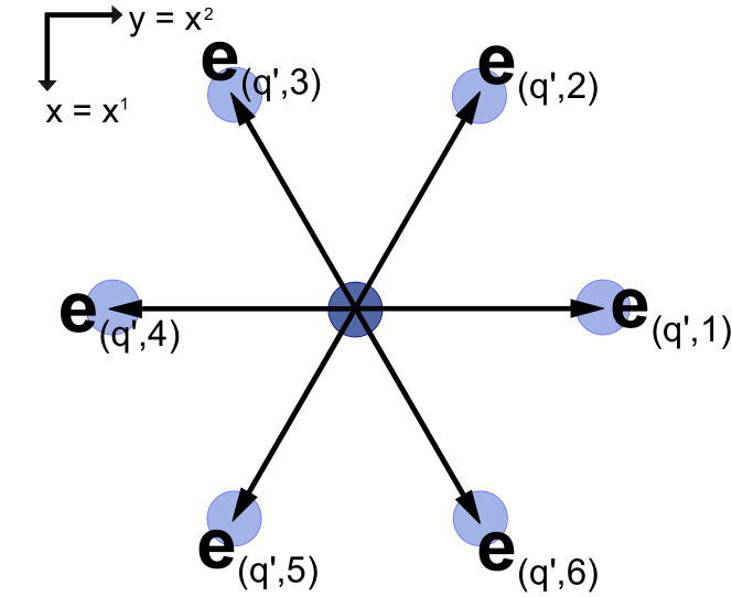
Figure 2: The populations $f_{\mathbf{q}}$ are moved between the nodes of a hexagonal lattice which are linked by the vector $\vec{e}_{\mathbf{q}}\delta t$.

The exact quadrature relations, Eqs. (11) and (12), ensure that the moments up to second order are still represented exactly:

$$\langle p^{\alpha}\rangle_{(eq)}=\sum_{\mathbf{q}}\frac{\omega_{\mathbf{q}}}{w(\bar{p}_{\mathbf{q}})}f_{(eq),\mathbf{q}}p^{\alpha}_{\mathbf{q}}\quad,$$ (13a)

$$\langle p^{\alpha}p^{\beta}\rangle_{(eq)}=\sum_{\mathbf{q}}\frac{\omega_{\mathbf{q}}}{w(\bar{p}_{\mathbf{q}})}f_{(eq),\mathbf{q}}p^{\alpha}_{\mathbf{q}}p^{\beta}_{\mathbf{q}}\quad.$$ (13b)

We have expanded and discretized the Fermi-Dirac equilibrium distribution for ultrarelativistic particles. Now, we will proceed to discretize the Boltzmann equation and find the evolution equation for the non-equilibrium distribution.

II.3 Lattice Boltzmann algorithm

With the expanded distribution functions and the discretization of momentum space at hand, we may use the following discrete Boltzmann equation He and Luo (1997b); Romatschke et al. (2011); Mendoza et al. (2010b),

$$f_{\mathbf{q}}(t+\delta t,\vec{x}+\vec{e}_{\mathbf{q}}\delta t)-f_{\mathbf{q}}(t,\vec{x})=-\frac{p^{\alpha}U_{\alpha}}{p^{0}\tau}(f_{\mathbf{q}}(t,\vec{x})-f_{eq,\mathbf{q}}(t,\vec{x})),$$ (14)

where we have introduced the notations $\vec{e}_{\mathbf{q}}=\vec{p}_{\mathbf{q}}/p^{0}$, and $f_{\mathbf{q}}(t,\vec{x})=f(t,\vec{x},p_{\mathbf{q}})$. Note that $\vec{e}_{\mathbf{q}}$ are unit vectors, which means that there are effectively $6$ different $\vec{e}_{\mathbf{q}}$. The discrete Boltzmann equation is now embedded into a lattice, and each time step of $\delta t=1$ corresponds to one execution of the following steps:

1. Calculate the equilibrium distributions $f_{eq,\mathbf{q}}(t,\vec{x})$ from Eq. (9) using the macroscopic variables $n=n(t,\vec{x})$, $\vec{u}=\vec{u}(t,\vec{x})$, and $T(t,\vec{x})$. At $t=0$, $n(t=0,\vec{x})$, $T(t=0,\vec{x})$, and $\vec{u}(t=0,\vec{x})$ are imposed as initial conditions.

2. Collision: Introducing the post-collisional distributions $f^{\prime}_{\mathbf{q}}$, calculate

   $$f^{\prime}_{\mathbf{q}}(t,\vec{x})=f_{\mathbf{q}}(t,\vec{x})-\frac{p^{\alpha}U_{\alpha}}{p^{0}\tau}(f_{\mathbf{q}}(t,\vec{x})-f_{eq,\mathbf{q}}(t,\vec{x})).$$

   At $t=0$, take $f_{\mathbf{q}}=f_{eq,\mathbf{q}}$.

3. Streaming: Move the $f^{\prime}_{\mathbf{q}}$ along $\vec{e}_{\mathbf{q}}$:

   $$f_{\mathbf{q}}(t+1,\vec{x}+\vec{e}_{\mathbf{q}})=f^{\prime}_{\mathbf{q}}(t,\vec{x})$$

4. Calculate the new macroscopic variables. First we compute the energy density of the system by solving the eigenvalue problem, $\langle p^{\alpha}p^{\beta}\rangle U_{\alpha}=\epsilon U^{\beta}$, according to the Landau-Lifshitz decomposition Cercignani and Kremer (2002). From this, we get $\epsilon$ and $U^{\alpha}$. Next, we use the relation $n=\langle p^{\alpha}\rangle U_{\alpha}=n$ to obtain the particle density. Here, the average values, $\langle p^{\alpha}\rangle$ and $\langle p^{\alpha}p^{\beta}\rangle$, are simply

   $$\langle p^{\alpha}\rangle = \sum_{\mathbf{q}}\frac{\omega_{\mathbf{q}}}{w(\bar{p}_{\mathbf{q}})}f_{\mathbf{q}}p^{\alpha}_{\mathbf{q}}\quad,$$

   $$\langle p^{\alpha}p^{\beta}\rangle = \sum_{\mathbf{q}}\frac{\omega_{\mathbf{q}}}{w(\bar{p}_{\mathbf{q}})}f_{\mathbf{q}}p^{\alpha}_{\mathbf{q}}p^{\beta}_{\mathbf{q}}\quad.$$

The streaming step indicates that if we discretize the real space based on a hexagonal lattice where the sites are linked by $\vec{e}_{\mathbf{q}}\delta t$, as shown in Fig. 2, the values of $f_{\mathbf{q}}$ will be moved between these sites exactly. This is known as “exact streaming” and crucial for the computational efficiency and accuracy of the lattice Boltzmann methods, because it removes any spurious numerical diffusivity.

In summary, we have developed a (2+1)-dimensional relativistic lattice Boltzmann scheme with the remarkable feature that it takes into account the Fermi-Dirac statistics, while recovering all the moments up to second order. The discretization is realized on a hexagonal lattice such that exact streaming is achieved. The fact that the quadrature corresponds to a hexagonal lattice allows to represent complex boundaries more precisely in graphene applications. This will be studied in more details in future works.

Up to now, we are working with undoped graphene, $\mu=0$. However, by using the same orthogonal polynomials, we can easily integrate the Fermi-Dirac statistics for the doped case, obtaining the extended formulation. In this work, we will use $\mu=0$, in order to compare the results with previous models in the literature that use the Maxwell-Jüttner distribution, since transport theory shows that in the case of undoped Fermi-Dirac statistics, the transport coefficients, namely shear viscosity and thermal conductivity, have the same expresions than for the Boltzmann statistics Cercignani and Kremer (2002). Therefore, the shear viscosity takes the value of $\eta=(3/5)P(\tau-\delta t/2)$ Mendoza et al. (2013c). Later, we will use the doped case to study the Riemann problem, which to best of our knowledge has never been studied before. However, it is present when, for instance, laser beams are pointed to the graphene sheet in order to measure transport coefficients Lee et al. (2011).

III Validation: Riemann problem

In order to validate our model, we solve the Riemann problem for the ultrarelativistic Fermi-Dirac gas. The Riemann problem is a standard test for both, relativistic and non-relativistic hydrodynamics numerical schemes, because it involves the evolution of two states of the fluid initially separated by a discontinuity. In our case, we set up an effectively one-dimensional system of $L_{x}\times L_{y}=3000\times 2$ nodes, using periodic boundary conditions in $x$ and $y$ components. Initially, there are two regions with particle densities, $n_{0}=1$ ($3L_{x}/4>x>L_{x}/4$), and $n_{1}=0.41$ ($x\leq L_{x}/4$ and $x\geq 3L_{x}/4$) creating a rectangular plateau of non-zero particle density in the center of the simulation zone. Here we consider and initial constant temperature, $T_{0}=1$. The initial velocity is set to zero and the value of the relaxation time $\tau$ is calculated for two different values of $\xi=\eta/(P_{0}\delta t)$, with $P_{0}=\frac{9\zeta(3)}{\pi^{2}}n_{0}T_{0}$. The evolution of the system is displayed in Fig. 3 after $470$ time steps, showing the generated shock wave. We have only plotted the region $x>L_{x}/2$ since the other one does not give additional information. Note that there is excellent agreement with the solutions provided by the model proposed in Ref. Mendoza et al. (2013b) for the same initial conditions.

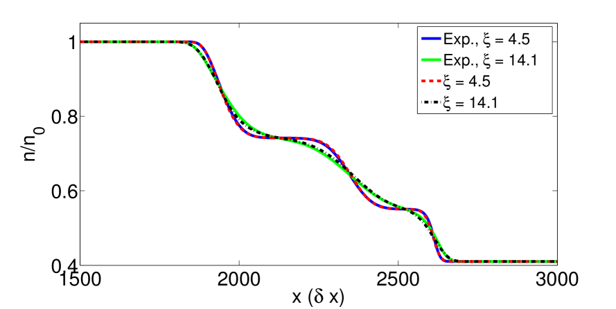
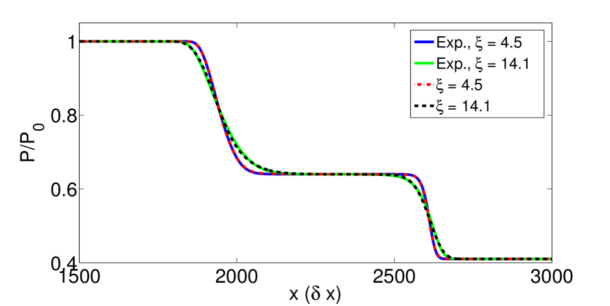
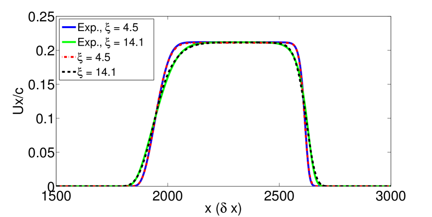
Figure 3: Density, pressure and velocity profile for the solution of the Riemann problem. Here $\xi=\eta/(P_{0}\delta t)$ is a dimensionless number. The expected results were calculated using the model in Ref. Mendoza et al. (2013b).

IV Riemann problem with $\mu\neq 0$

Let us now consider the case when the chemical potential $\mu$ is different from zero. For this purpose, we follow the same procedure described before but this time, we keep $\mu\neq 0$. The development is straightforward, and therefore does not deserve a full explanation. The polynomials are the same as described in Appendix A, and the coefficients $a^{(nk)}_{\underline{i}}$ are calculated by using Eq. (8).

The hydrodynamic approach of electrons in graphene works for low doping, $\mu/k_{B}T\ll 1$ Müller and Sachdev (2008); Fritz et al. (2008); Müller et al. (2008). Therefore, we can expand the discrete equilibrium distribution in powers of $\mu/k_{B}T$ up to third order, neglecting errors of the order of $(\mu/k_{B}T)^{4}$. We perform additional simulations of the Riemann problem with the same parameters as before, but now, varying the chemical potential.

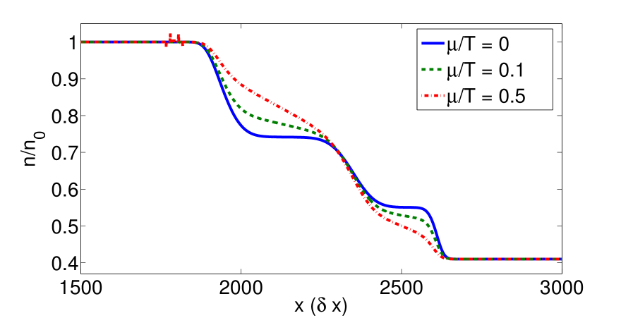
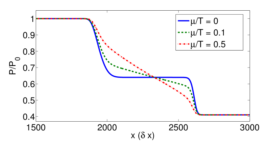
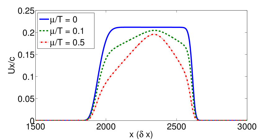
Figure 4: Density, pressure and velocity profile of the solution of the Riemann problem, for different values of the chemical potential $\mu$.

As we can observe from Fig. 4, increasing the chemical potential tends to increase also the effective viscosity of the system, smoothing the profiles of the velocity, pressure and density. This result is very interesting because it suggest that, in fact, impurities with soft potentials (small $\mu/k_{B}T$) in graphene samples can be treated as local modifications in the effective viscosity of the electronic fluid. In other words, this result suggests a promissing way to include impurities in the hydrodynamic approach of electrons in graphene. Note that in this figure, there is a noise in the profile of the particle density. This numerical instability remains with the same amplitude and is always located at the boundary when $n=n_{0}$, and therefore, it does not destroy the stability of the simulation. It can be due to the relevance of higher order terms which are not recovered by our expansion.

V Conclusions

We have derived a new family of orthogonal polynomials using as weight function the Fermi-Dirac distribution for ultrarelativistic particles in two dimensions. By applying the Gaussian quadrature we have calculated the set of representative momentum (2+1)-vectors, which allows us to replace the integrals over the continuum momentum space by sums over such vectors. As a very interesting result, we have found that those vectors possess the same symmetries than the honeycomb lattice of carbon atoms in graphene, making possible the accurate implementation of complex boundary conditions in future applications, such as point defects and nanoribbons. The derivation has been performed by imposing that the expanded distribution should fulfill at least the first three moments of the equilibrium distribution, which are needed to recover the appropriate hydrodynamics. However, higher order moments can also be recovered by using the same procedure in this paper.

In addition, we have developed a new lattice kinetic scheme to study the dynamics of the electronic flow in graphene. The model is validated on the Riemann problem, which is one of the most challenging tests in numerical hydrodynamics, presenting excellent agreement with previous models in the literature. By increasing the chemical potential, we have found that the profiles of velocity, particle density, and pressure, change similar to the case when the viscosity is increased, concluding that increasing the Fermi energy results in increasing the effective viscosity of the electronic fluid. This result suggests that soft impurities in graphene samples can be treated as local modifications of the viscosity, however, further studies must be performed in order to confirm this statement.

The fact that we can propagate the information from one site to another in an exact way, avoiding interpolation, removes any kind of spurious numerical diffusivity. Therefore, we expect this model to be appropriated to study many problems in electronic transport in graphene in the framework of the hydrodynamic approach, e.g. turbulence and hydrodynamical instabilities in graphene flow, just to name a few.

Extensions of the present model to take into account higher order moments of the Fermi-Dirac equilibrium distribution as well as the inclusion of the distribution and dynamics of holes, will be a subject of future research.

Appendix A Polynomials and $\Gamma$-constants

In this section, we write explicitly the family of polynomials, which are orthogonal using as weighting function the Fermi-Dirac distribution at rest, with their respective normalization factors. For the case of the angular dependence, we have

$$P^{(0)}(\vec{v}) = 1$$

$$P^{(1)}_{i}(\vec{v}) = v_{i}$$

$$P^{(2)}_{ij}(\vec{v}) = v_{i}v_{j}-\frac{1}{2}\delta_{ij}$$

with normalization factors,

$$\Gamma_{P}^{(0)} = 1$$

$$\Gamma_{P,ij}^{(1)} = \frac{1}{2}\delta_{ij}$$

$$\Gamma_{P,ijkl}^{(2)} = \frac{1}{8}\left(\delta_{il}\delta_{jk}+\delta_{ik}\delta_{jl}-\delta_{ij}\delta_{kl}\right)\quad.$$

For the case of the radial dependence, we have the polynomials

$$F^{(0)}(\bar{p}) = 1$$

$$F^{(1)}(\bar{p}) = \bar{p}-c_{10}\quad,$$

$$c_{10} = \frac{\pi^{2}}{12\log(2)}\quad,$$

$$F^{(2)}(\bar{p}) = \bar{p}^{2}-c_{21}\bar{p}-c_{20}\quad,$$

$$c_{21} = -\frac{6(7\pi^{4}\log(2)-15\pi^{2}\zeta(3))}{5(\pi^{4}-216\log(2)\zeta(3))}\quad,$$

$$c_{20} = \frac{7\pi^{6}-3240\zeta(3)^{2}}{10(\pi^{4}-216\log(2)\zeta(3))}\quad,$$

with $\zeta$ denoting the Riemann zeta function. The normalization factors for these polynomials are:

$$\Gamma_{F}^{(0)} = \frac{\log(2)}{4\pi}\quad,\quad\Gamma_{F}^{(1)}=-\frac{\pi^{3}}{576\log(2)}+\frac{3\zeta(3)}{8\pi}\quad,$$

$$\Gamma_{F}^{(2)} = \frac{1}{400\pi}\biggl{(}\frac{49\pi^{8}\log(2)-210\pi^{6}\zeta(3)+48600\zeta(3)^{3})}{\pi^{4}-216\log(2)\,\zeta(3)}$$

$$+ 2250\zeta(5)\biggr{)}\quad.$$

Appendix B Coefficients for the expansion of $f_{eq}$ and relation to moments

The coefficients of the expansion in Eq. (9) are given by

$$a^{(00)} = \theta\quad,\quad a^{(10)}_{i}=2\,\theta\frac{1}{\gamma+1}\,u_{i}\gamma\quad,$$

$$a^{(20)}_{ij} = \sigma_{ij}\,4\,\theta\frac{1}{(\gamma+1)^{2}}\left[\gamma^{2}(u_{i}u_{j}-\tfrac{1}{2}\delta_{ij})\gamma^{2}+\tfrac{1}{2}\delta_{ij}\right]\quad,$$

$$a^{(01)} = \alpha^{(1)}\theta\left[\theta\gamma-1\right]\quad,$$

$$a^{(11)}_{i} = \frac{2\alpha^{(1)}\theta}{\gamma+1}\left[\theta(\gamma+1)-1\right]\,u_{i}\gamma\quad,$$

$$a^{(21)}_{ij} = \frac{4\alpha^{(1)}\theta}{(\gamma+1)^{2}}\left[(2-\delta_{ij})\theta(\gamma+2)-\sigma_{ij}\right][\gamma^{4}(u_{i}u_{j}-\delta_{ij}/2)$$

$$+ \delta_{ij}/2]\quad,$$

$$a^{(02)} = \alpha^{(2)}\theta\,\big{[}\beta^{(2|1)}(\theta\gamma-1)+\beta^{(2|2)}((3\theta\gamma-2)-\theta)$$

$$+ \beta^{(2|3)}(\theta^{2}(3\gamma^{2}-1)-2)\big{]}\quad,$$

$$a^{(12)}_{i} = \frac{2\alpha^{(2)}\theta}{\gamma+1}\big{[}\beta^{(2|1)}(\theta(\gamma+1)-1)$$

$$+ \beta^{(2|2)}\theta(3\theta\gamma-2)(\gamma+1)$$

$$+ \beta^{(2|3)}(3\theta^{2}\gamma(\gamma+1)-2)\big{]}u_{i}\,\gamma\quad,$$

$$a^{(22)}_{ij} = \frac{4\alpha^{(2)}\theta}{(\gamma+1)^{2}}\big{[}\beta^{(2|1)}((2-\delta_{ij})\theta(\gamma+2)-(2\delta_{ij}+1)\sigma_{ij})$$

$$+ \beta^{(2|2)}(3\theta^{2}(\gamma+1)^{2}-2(2-\delta_{ij})(\theta(\gamma+2)-2\delta_{ij}\sigma_{ij}))$$

$$+ \beta^{(2|3)}(3\theta^{2}(\gamma+1)^{2}-2\sigma_{ij})\big{]}[\gamma^{2}(u_{i}u_{j}-\tfrac{1}{2}\delta_{ij})\gamma^{2}$$

$$+ \tfrac{1}{2}\delta_{ij}]\quad,$$

where $\sigma_{ij}=(-1)^{\delta_{2,i}\delta_{2,j}}$ or

$$(\sigma_{ij})=\left(\begin{array}[]{cc}1&1\\ 1&-1\end{array}\right)\quad,$$ (15)

and,

$$\alpha^{(1)} = \frac{12\pi^{2}\log(2)}{216\log(2)\zeta(3)-\pi^{4}}\quad,$$

$$\alpha^{(2)} = 5\,[2250\zeta(5)(216\log(2)\zeta(3)-\pi^{4})+210\pi^{6}\zeta(3)$$

$$- 49\pi^{8}\log(2)-48600\zeta(3)^{3}]^{-1}\quad,$$

$$\beta^{(2|1)} = -14\pi^{6}\log(2)\quad,$$

$$\beta^{(2|2)} = -15\pi^{4}\zeta(3)^{2}\quad,$$

$$\beta^{(2|3)} = 3240\log(2)\zeta(3)^{2}\quad,$$

which are approximately, $\alpha^{(1)}\approx 0.994$, $\alpha^{(2)}\beta^{(2|1)}\approx-1.629$, $\alpha^{(2)}\beta^{(2|2)}\approx-0.307$, and $\alpha^{(2)}\beta^{(2|1)}\approx 0.567$.

To obtain the moments from the expansion of $f_{eq}$, we expressed them in terms of the $a^{(nk)}_{\underline{i}}$ using Eqs. (8), (9), and the expressions in Appendix A, e.g. $\langle p^{0}\rangle=T_{0}^{2}\left(\Gamma_{F}^{(1)}a^{(01)}+c_{10}\Gamma_{F}^{(0)}a^{(00)}\right)$.

Note that for the calculation of the coefficients $a^{(nk)}_{\underline{i}}$ we should use of the integration formula

$$\int_{0}^{\infty}\text{d}x\frac{x^{n-1}}{z^{-1}\text{e}^{a\,x}+1}=-z^{-1}a^{-n}\Gamma(n)\operatorname{Li}_{n}(-z)\quad,$$

which holds for $n>0$, $a\in\mathbb{R}$, $a>0$. Here, $\Gamma(n)$ denotes the gamma function, which becomes $\Gamma(n)=(n-1)!$ for $n\in\mathbb{N}$. $\operatorname{Li}_{n}(z)$ is the polylogarithm which can be defined using a power series: $\operatorname{Li}_{n}(z)=\sum_{k=1}^{\infty}\frac{z^{k}}{k^{n}}$. If we consider the chemical potential in the Fermi-Dirac distribution to be zero, we have $z=1$ and the relevant values of the polylogarithm become $\operatorname{Li}_{1}(-1)=-\log(2),\,\operatorname{Li}_{2}(-1)=-\frac{\pi^{2}}{12},\,\operatorname{Li}_{3}(-1)=-\frac{3}{4}\zeta(3)$. On the other hand, for $\mu\neq 0$, we take $z=e^{\mu/T}$.

Appendix C Results for radial Gaussian quadrature

When the radial Gaussian quadrature is applied, the following values for the discrete $\bar{p}_{i}$ are obtained:

$$\bar{p}_{1} = 0.4840534751554060637550794361591\quad,$$

$$\bar{p}_{2} = 2.4467448689670852668751189804200\quad,$$

$$\bar{p}_{3} = 6.4243522612255152565859012563254\quad,$$

with its respective weight functions

$$\omega^{(\bar{p})}_{1} = 0.0368730611359638360101542425978\quad,$$

$$\omega^{(\bar{p})}_{2} = 0.0175666801777458993453757617390\quad,$$

$$\omega^{(\bar{p})}_{3} = 0.0007191587244531629935841036927\quad.$$

References

- Novoselov et al. (2005) K. Novoselov, A. Geim, S. Morozov, D. Jiang, M. Katsnelson, I. Grigorieva, and S. Dubonos, Nature Letters 438, 197 (2005).
- Novoselov et al. (2004) K. S. Novoselov, A. K. Geim, S. V. Morozov, D. Jiang, Y. Zhang, S. V. Dubonos, I. V. Grigorieva, and A. A. Firsov, Science 306, 666 (2004).
- DiVincenzo and Mele (1984) D. P. DiVincenzo and E. J. Mele, Physical Review B 29, 1685 (1984).
- Das Sarma et al. (2011) S. Das Sarma, S. Adam, E. H. Hwang, and E. Rossi, Rev. Mod. Phys. 83, 407 (2011).
- Geim and MacDonald (2007) A. K. Geim and A. H. MacDonald, Phys. Today , 35 (2007).
- Müller et al. (2009) M. Müller, J. Schmalian, and L. Fritz, Physical Review Letters 103, 025301 (2009).
- Müller and Sachdev (2008) M. Müller and S. Sachdev, Phys. Rev. B 78, 115419 (2008).
- Fritz et al. (2008) L. Fritz, J. Schmalian, M. Müller, and S. Sachdev, Phys. Rev. B 78, 085416 (2008).
- Müller et al. (2008) M. Müller, L. Fritz, and S. Sachdev, Phys. Rev. B 78, 115406 (2008).
- Müller et al. (2009) M. Müller, J. Schmalian, and L. Fritz, Phys. Rev. Lett. 103, 025301 (2009).
- Mendoza et al. (2011) M. Mendoza, H. J. Herrmann, and S. Succi, Phys. Rev. Lett. 106, 156601 (2011).
- Mendoza et al. (2013a) M. Mendoza, H. J. Herrmann, and S. Succi, Sci. Rep. 3, 1052 (2013a).
- Mendoza et al. (2010a) M. Mendoza, B. M. Boghosian, H. J. Herrmann, and S. Succi, Phys. Rev. Lett. 105, 014502 (2010a).
- Mendoza et al. (2010b) M. Mendoza, B. M. Boghosian, H. J. Herrmann, and S. Succi, Phys. Rev. D 82, 105008 (2010b).
- Hupp et al. (2011) D. Hupp, M. Mendoza, I. Bouras, S. Succi, and H. J. Herrmann, Phys. Rev. D 84, 125015 (2011).
- Xu and Greiner (2005) Z. Xu and C. Greiner, Phys. Rev. C 71, 064901 (2005).
- Bouras et al. (2009) I. Bouras, E. Molnar, H. Niemi, Z. Xu, A. El, O. Fochler, C. Greiner, and D. H. Rischke, Phys. Rev. Lett. 103, 032301 (2009).
- Romatschke et al. (2011) P. Romatschke, M. Mendoza, and S. Succi, Phys. Rev. C 84, 034903 (2011).
- Cercignani and Kremer (2002) C. Cercignani and G. M. Kremer, The Relativistic Boltzmann Equation: Theory and Applications (Boston; Basel; Berlin: Birkhauser, 2002).
- He and Luo (1997a) X. He and L.-S. Luo, Phys. Rev. E 56, 6811 (1997a).
- Martys et al. (1998) N. S. Martys, X. Shan, and H. Chen, Phys. Rev. E 58, 6855 (1998).
- He and Luo (1997b) X. He and L.-S. Luo, Physical Review E 55, R6333 (1997b).
- Succi (2001) S. Succi, The lattice Boltzmann equation for fluid dynamics and beyond (Clarendon Press and Oxford University Press, Oxford and New York, 2001).
- Mendoza et al. (2013b) M. Mendoza, I. Karlin, S. Succi, and H. J. Herrmann, Phys. Rev. D 87, 065027 (2013b).
- Han et al. (2007) M. Y. Han, B. Özyilmaz, Y. Zhang, and P. Kim, Phys. Rev. Lett. 98, 206805 (2007).
- Barone et al. (2006) V. Barone, O. Hod, and G. E. Scuseria, Nano Letters 6, 2748 (2006).
- Jüttner (1928) F. Jüttner, Z. Physik (Zeitschrift für Physik) 47, 542 (1928).
- Grad (1949) H. Grad, Communications on Pure and Applied Mathematics 2, 331 (1949).
- Davis and Rabinowitz (1984) P. J. Davis and P. Rabinowitz, Methods of numerical integration, 2nd ed. (Academic Press, Orlando, 1984).
- Mendoza et al. (2013c) M. Mendoza, I. Karlin, S. Succi, and H. J. Herrmann, JSTAT 2013, P02036 (2013c).
- Lee et al. (2011) J.-U. Lee, D. Yoon, H. Kim, S. W. Lee, and H. Cheong, Phys. Rev. B 83, 081419 (2011).