Non-Gaussian Fluctuation and Non-Markovian Effect in the Nuclear Fusion Process: Langevin Dynamics Emerging from Quantum Molecular Dynamics Simulations

Abstract

Macroscopic parameters as well as precise information on the random force characterizing the Langevin type description of the nuclear fusion process around the Coulomb barrier are extracted from the microscopic dynamics of individual nucleons by exploiting the numerical simulation of the improved quantum molecular dynamics. It turns out that the dissipation dynamics of the relative motion between two fusing nuclei is caused by a non-Gaussian distribution of the random force. We find that the friction coefficient as well as the time correlation function of the random force takes particularly large values in a region a little bit inside of the Coulomb barrier. A clear non-Markovian effect is observed in the time correlation function of the random force. It is further shown that an emergent dynamics of the fusion process can be described by the generalized Langevin equation with memory effects by appropriately incorporating the microscopic information of individual nucleons through the random force and its time correlation function.

The fusion of two nuclei is one of the major non-equilibrium processes in low energy nuclear reactions where the fluctuation and dissipation play important roles. It is rather difficult to describe the fusion process without significant simplifications. Under various assumptions, several macroscopic transport models have been introduced to evaluate the formation of a compound nucleus in heavy-ion fusion reactions Shen et al. (2002); *Zagrebaev2012_PRC85-014608; *Aritomo2012_PRC85-044614; *Siwek-Wilczynska2012_PRC86-014611; *Liu2013_PRC87-034616; Adamian et al. (1998); *Li2010_NPA834-353c; *Gan2011_SciChinaPMA54S1-61; *Nasirov2011_PRC84-044612; *Wang2012_PRC85-041601R. However, the microscopic mechanism on how two colliding nuclei fuse, especially how the relevant kinetic energy dissipates into the intrinsic degrees of freedom (DoF), remains a subject requiring further research.

On the other hand, it is becoming feasible to get various information out of microscopic numerical simulations, like time-dependent Hartree-Fock (TDHF) theories Bonche et al. (1976); Guo et al. (2007); *Guo2008_PRC77-041301R; Washiyama and Lacroix (2008); Washiyama et al. (2009); Simenel (2012), the many-body correlation transport (MBCT) theory Wang and Cassing (1985), the quantum molecular dynamics (QMD) Aichelin (1991), the antisymmetrized molecular dynamics Ono (1999), and the fermion molecular dynamics Feldmeier and Schnack (2000). The TDHF theory is mainly based on the mean-field concept; in TDHF, fluctuations of collective variables are considerably underestimated. Much effort has been made to give a beyond-mean-field description of fluctuations Ayik (2008). The $n$-body correlations are incorporated in the MBCT theory Wang and Cassing (1985) which has only been used in very light systems Liu et al. (1996).

The QMD is a microscopic dynamical $n$-body theory which was successfully used in intermediate-energy heavy-ion collisions (HIC) Aichelin (1991). An improved QMD (ImQMD) has been developed in order to extend the application of QMD to low-energy HICs near the Coulomb barrier Wang et al. (2002); *Wang2004_PRC69-034608. A series of improvements were made in the ImQMD; in particular, by using the phase space occupation constraint method Papa et al. (2001), the fermionic properties of nucleons is remedied, which is important for low-energy collisions. Making full use of the microscopic information provided by ImQMD simulations, in this Letter, we try to understand how the macroscopic fusion dynamics emerges out of the microscopic one.

We focus on a simplest case of symmetric fusion process with the impact parameter equal to zero. In this case, the system can be divided into the left- and right-half parts instead of a projectile and a target Ayik et al. (2009). The relative motion between two centers of mass (CoM) of the left and right parts is chosen as the relevant DoF to be described by the Langevin equation. Our analysis is limited in a stage where the relative distance ${R}$ is much larger than its width.

The one-dimensional generalized Langevin equation with memory effects reads Mori (1965); Sakata et al. (2011); Frobrich and Gontchar (1998)

$$\frac{du(t)}{dt}=-\int_{-\infty}^{t}\gamma(t-t^{\prime})u(t^{\prime})dt^{\prime}+\frac{1}{\mu}{\delta F}(t)-\frac{1}{\mu}\frac{dV({R})}{{d{R}}},~{}$$ (1)

where $u(t)$ is the relative velocity between the two parts, $\delta F(t)$ the random force felt by either part, $\mu$ the reduced mass of the system, $\gamma(t-t^{\prime})$ the friction kernel, and $V(R)$ the potential for the relative motion.

In the ImQMD model Wang et al. (2002, 2004), a trial wave function is restricted within a parameter space $\{\textbf{r}_{j},\textbf{p}_{j}\}$, where $\textbf{r}_{j}$ and $\textbf{p}_{j}$ are mean values of position and momentum operators of the $j$th nucleon which is expressed by a Gaussian wave packet. The time evolution of the trial wave function under an effective potential is governed by the time-dependent variational principle Aichelin (1991); Ono (1999); Feldmeier and Schnack (2000). An expectation value of the Hamiltonian is given by using an improved Skyrme potential energy density functional. In this Letter, we concentrate on head-on collisions of ⁹⁰Zr+⁹⁰Zr. Ten thousand collision events were simulated. Each simulation is started at ${R}={R}_{0}=30$ fm and with an incident energy $E=195$ MeV. Numerical details can be found in Refs. Tian et al. (2008); *Zhao2009_PRC79-024614.

The potential for the relative motion is defined as,

$$V({R})=E_{\mathrm{tot}}({R})-E_{\mathrm{left}}({R})-E_{\mathrm{right}}({R}),~{}$$ (2)

where $E_{\mathrm{tot}}$, $E_{\mathrm{left}}$, and $E_{\mathrm{right}}$ represent the energy of the system and those of the left and right parts, respectively; each of which consists of the kinetic energy, the nuclear and the Coulomb potential energies. The potential $V(R)$ is shown in Figs. 1 and 3. The TDHF has also been used to extract microscopic interaction potentials between two nuclei Umar and Oberacker (2006); Washiyama and Lacroix (2008) which show similar features as those from the ImQMD simulations presented here and in Refs. Jiang et al. (2010); *Zanganeh2012_PRC85-034601.

The random force or the fluctuation of force in the $i$th event is defined as

$${\delta F(x)}_{i} \equiv F_{i}(x)-\langle F(x)\rangle,\ \ x=t\ \mathrm{or}\ {R},$$ (3)

where $F_{i}(x)\equiv\sum_{j=1}^{A}f^{j}_{i}(x)$ denotes the total force acting on the left (right) part of the system in the $i$th event, $\langle F(x)\rangle\equiv\frac{1}{n}\sum_{i=1}^{n}F_{i}(x)$ the mean value, and $f^{j}_{i}(x)$ the force on the $j$th nucleon in the left (right) part. Here $A$ means the number of nucleons contained in the left (right) part and $n$ denotes the total number of events. In Eq. (3) and hereafter, $\langle{Q}\rangle$ denotes an average of ${Q}$ over all events. For low-energy collisions, the fluctuation mainly stems from the initialization of each event in which the position and the momentum of each particle are chosen randomly under certain conditions. With time this initial fluctuation propagates and is not smoothed out because in QMD a many-body rather than a mean field problem is solved Aichelin (1991).

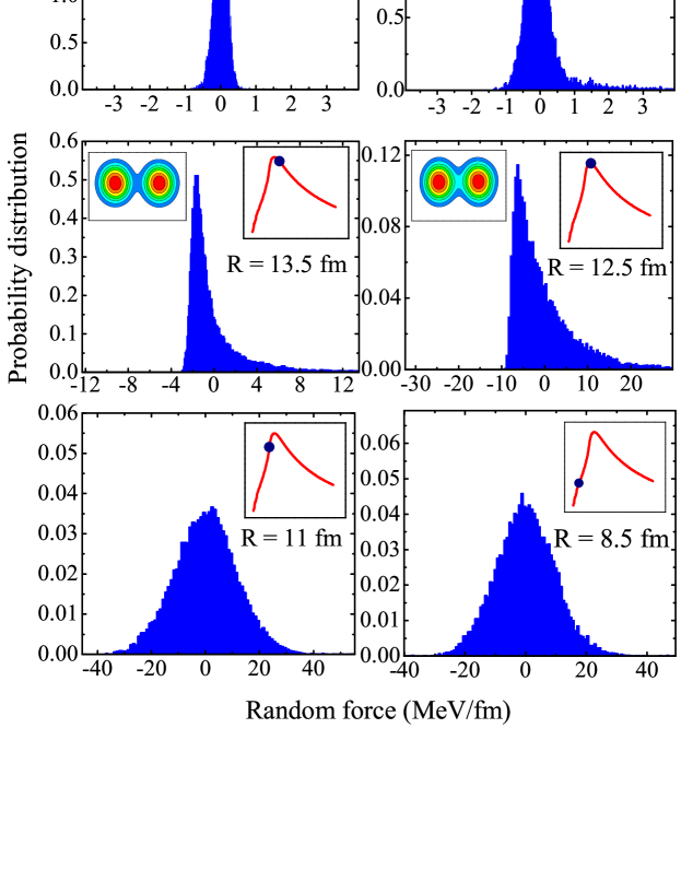
Figure 1: (color online) Distributions of the random force ${\delta F}({R})$. Each inset shows the potential $V({R})$ with the blue dot representing the position where the system locates. The contour plots display the nucleon density distribution of the system.

Distributions of ${\delta F}({R})$ at several distances are shown in Fig. 1. The random force at ${R}(t=0)={R}_{0}$ shows a Gaussian distribution with the full width at half maximum (FWHM) $\Gamma\approx$ 0.1 MeV/fm which could be understood analytically as only the Coulomb field is felt by the particles. In a region far away from the barrier, e.g., ${R}\approx 18$ fm, ${\delta F}$ has a Gaussian distribution with $\Gamma\approx 0.5$ MeV/fm. From a certain distance, ${R}\approx 13.5$ fm, there appears a non-Gaussian shape, as is observed in Fig. 1. According to the shape of the distribution of ${\delta F}({R})$, one may divide the whole process into three regions. Region 1 represents an approaching phase up to the touching point: The distribution has a Gaussian form with a rather narrow width. Region 2 is from the touching point to the barrier top: A non-Gaussian shape appears. Region 3 is from just inside the barrier top to the fusing phase: The distribution of ${\delta F}({R})$ has again a Gaussian shape with $\Gamma\approx 15$ MeV/fm which is almost two orders of magnitude larger than that in Region 1.

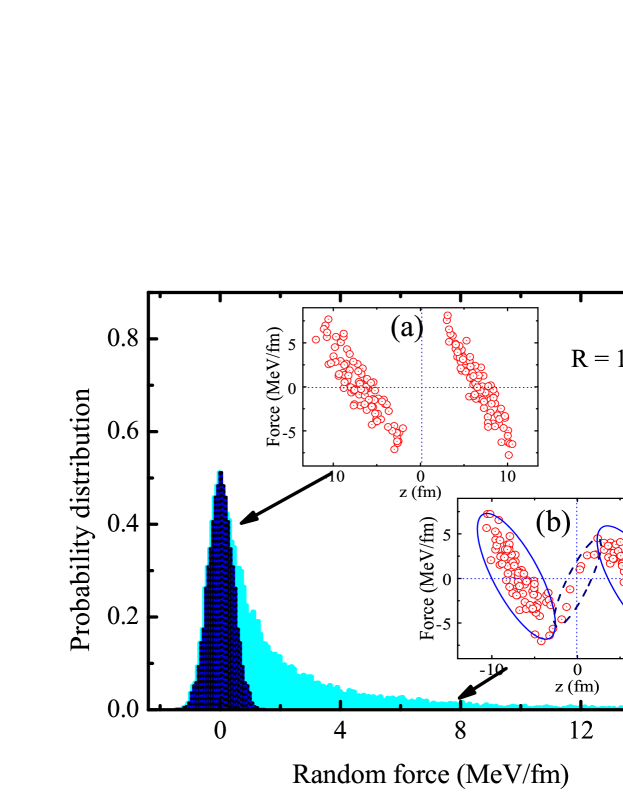
Figure 2: (color online) Distribution of the random force ${\delta F}({R})$ at ${R}=$ 13.5 fm which is divided into the symmetric Gaussian (dark blue) and asymmetric tail (light blue) parts. Two typical events are shown in the inset: The abscissa and the ordinate express relative position $z$ of each nucleon and the force it feels in the $z$ direction.

To make clear what happens in Region 2, we divide the distribution of ${\delta F}({R})$ into a symmetric Gaussian and an asymmetric tail parts as is shown in Fig 2. The width of the Gaussian part is of the same order of magnitude as that in Region 1. The detailed structure of the random force can be studied by examining the strength and direction of the force felt by each nucleon. One typical event in the symmetric part is shown in Fig. 2(a): All nucleons are well divided into two separated groups expressing the projectile and the target, respectively. Moreover, each nucleon locating in the left side of each nucleus feels a force toward the right (positive value), and that in the right side feels a force toward the left (negative value), so as to keep a stable mean-field. The resultant force made by all nucleons in each nucleus is almost zero. Namely, the intrinsic structure of two fusing nuclei is kept almost unchanged, so is the width of the random force. This situation persists in events which belong to the symmetric Gaussian part in Region 2 and in all those in Region 1.

A typical event in the asymmetric tail is shown in Fig. 2(b). Nucleons are roughly divided into two groups surrounded by solid lines. However, there appears a small third group within the dashed line. Since a few points in the negative (positive) force region express a set of nucleons which escape from the left (right) nucleus, and are being absorbed by the right (left) nucleus, a resultant force made by these nucleons gives a large right(left)-directed component to the random force. These transferred nucleons move in an average potential formed by both the projectile and the target; they play a role to open a window.

When the two nuclei come much closer, there occur more events which have more nucleons in the third group. Meanwhile, the other two groups, originating from the projectile and target, become closer to each other. Consequently, the asymmetric tail in the distribution of ${\delta F}({R})$ becomes larger. At the border between Regions 2 and 3, it becomes very difficult to distinguish an event in the center part of the distribution from that in the tail part and all events are absorbed into a widely spreading Gaussian distribution.

From above discussions, it is concluded that the main microscopic origin of the random force, i.e., a two orders of magnitude enhancement of the random force is generated by individual nucleons in the third group. These nucleons also result in the abnormal behavior in the distribution of ${\delta F}({R})$, i.e., the long tail in Region 2 and a much larger width in Region 3 compared to Region 1.

Next let us extract information for the macroscopic dynamics out of microscopic simulations. Assuming that the work done by the friction force is completely converted into the intrinsic energy $E_{\mathrm{intr}}({R})$, one gets the friction coefficient $\gamma_{0}(R)$ from the Rayleigh formula Washiyama et al. (2009); Ayik et al. (2009); Frobrich and Gontchar (1998),

$$\gamma_{0}({R})\equiv\frac{\langle F_{\mathrm{fric}}({R})\rangle}{\langle P\rangle_{{R}}},~{}$$ (4)

with $F_{\mathrm{fric}}({R})\equiv dE_{\mathrm{intr}}({R})/d{R}$, $E_{\mathrm{intr}}({R})\equiv E_{\mathrm{tot}}({R})-E_{\mathrm{coll}}({R})$, and $E_{\mathrm{coll}}({R})={P^{2}}/{2\mu}+V({R})$. $P$ denotes the relative momentum between two CoMs and its mean value $\langle P\rangle_{{R}}$ at a given ${R}$ is defined as

$$\langle P\rangle_{{R}}\equiv\frac{1}{n}\sum_{i=1}^{n}\left.P_{i}(t_{i})\right|_{\{t_{i}|{R}_{i}(t_{i})={R}\}},$$ (5)

where $P_{i}(t)$ and ${R}_{i}(t)$ are the momentum and coordinate of the $i$-th event at time $t$ and the following correspondence is used: For each event $i$, a time $t_{i}$ is chosen in such a way that the relative distance takes a given value ${R}$, i.e., ${R}_{i}(t_{i})={R}$. A ${R}$-dependent correlation function is defined as

$$\langle{\delta F}({R}){\delta F}({R})\rangle\equiv\frac{1}{n}\sum_{i=1}^{n}\left.{\delta F}_{i}(t_{i}){\delta F}_{i}(t_{i})\right|_{\{t_{i}|{R}_{i}(t_{i})={R}\}}.$$ (6)

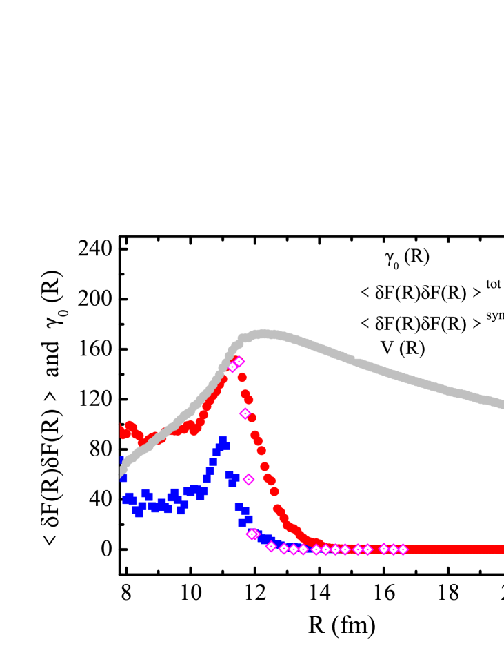
Figure 3:  (color online) The correlation function $\langle{\delta F}({R}){\delta F}({R})\rangle^{\mathrm{tot}}$ [red dots, in (MeV/fm)²] and the friction coefficient $\gamma_{0}({R})$ (blue squares, in $0.001~{}c$/fm). The grey line shows the potential $V({R})$. Pink diamonds represent $\langle{\delta F}({R}){\delta F}({R})\rangle^{\mathrm{sym}}$ calculated by eliminating events in the asymmetric tail.

Figure 3 shows the correlation function $\langle{\delta F}({R}){\delta F}({R})\rangle$ and the friction coefficient $\gamma_{0}({R})$ which play decisive roles in the macroscopic description of dissipation phenomena. As is seen from Fig. 3, $\langle{\delta F}({R}){\delta F}({R})\rangle$ and $\gamma_{0}({R})$ have similar shapes and their peaks locate at similar ${R}$. The friction coefficient of the fusion process induced by a head-on collision extracted from TDHF calculations shows similar strong peak structure. As the incident energy $E$ increases, the shape of the curve $\gamma_{0}(R)\sim R$ may change. When $E$ is high enough, $\gamma_{0}(R)$ increases gradually with decreasing $R$ Washiyama et al. (2009); Ayik et al. (2009); Wen et al. .

To explore more deeply the dynamical relation between the microscopic motion of individual nucleons and the macroscopic dissipative motion, in Fig. 4 we show the time correlation function of the random force ${\sigma}({R},\tau)$ which is defined as

$${\sigma}({R},\tau) \equiv \frac{1}{n}\sum_{i=1}^{n}\left.{\delta F}_{i}(t_{i}){\delta F}_{i}(t_{i}-\tau)\right|_{\{t_{i}|{R}(t_{i})={R}\}}.$$ (7)

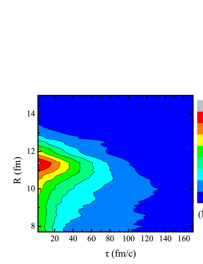
Figure 4: (color online) Time correlation function $\sigma(r,\tau)$ (7).

In Fig. 4 one clearly finds the non-Markovian effect. Especially when ${R}=12\sim 10$ fm, it is important to take account of memory effects generated by the microscopic motion of nucleons when one tries to properly evaluates macroscopic effects of the dissipation. Starting from the generalized Langevin equation (1) with memory effects, one gets a generalized fluctuation-dissipation (GFD) relation $\langle{\delta F}(t){\delta F}(t-t^{\prime})\rangle=\mu T\gamma(t-t^{\prime})$ which properly takes account of the time correlation of the random force. There are many ways to define the temperature for compound nuclei (see, e.g., Ref. Su et al. (2012)). Here we define an effective temperature for colliding systems by applying the GFD relation,

$$T_{\mathrm{non-Markov}}(R) = \frac{1}{\mu\gamma_{0}(R)}\int_{0}^{\infty}d\tau{\sigma}({R},\tau).$$ (8)

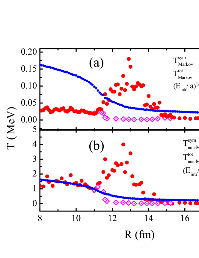
Figure 5: (color online) Effective temperature in the Markovian limit (a) and the Non-Markovian one (b). The blue line shows $\sqrt{E_{\textrm{intr}}/a}$ with $a=A_{\mathrm{total}}/4$.

The effective temperature $T_{\mathrm{non-Markov}}^{\textrm{tot}}$ as well as the one from the Markovian approximation $T_{\mathrm{Markov}}^{\textrm{tot}}$ are shown in Fig. 5. $\sqrt{E_{\mathrm{intr}}/a}$ representing the temperature of a compound nucleus in the Fermi gas model is also shown as a reference. Although $T_{\mathrm{non-Markov}}^{\textrm{tot}}$ and $T_{\mathrm{Markov}}^{\textrm{tot}}$ differ by one order of magnitude, they both show a peak around the range where the asymmetric tail appears in the distribution of ${\delta F}({R})$. These peaks are related to the fact that the relative motion for events in the asymmetric tail part of the $\delta F(R)$ distribution is strongly affected by a few transferred nucleons between two fusing nuclei, i.e., by those in the third group of Fig. 2(b). The macroscopic dynamics of the relative motion described by the one-dimensional Langevin equation (1) is not appropriate in Region 2. In other words, the appearance of the non-Gaussian distributed random force indicates a necessity of introducing a new macroscopic DoF. Whether or not this new DoF may be related to the formation of a neck is an open question Siwek-Wilczynska et al. (2012); *Zagrebaev2012_PRC85-014608; *Shen2002_PRC66-061602R; *Aritomo2012_PRC85-044614; *Liu2013_PRC87-034616; Adamian et al. (1997); *Adamian2000_NPA671-233; *Diaz-Torres2000_PLB481-228.

After eliminating the events in the asymmetric tail in the distribution of ${\delta F}({R})$, one gets effective temperatures $T_{\mathrm{non-Markov}}^{\textrm{sym}}$ and $T_{\mathrm{Markov}}^{\textrm{sym}}$ which are depicted in Fig. 5. The correlation function $\langle\delta F(R)\delta F(R)\rangle$ after eliminating the asymmetric tail is also shown in Fig. 3. $T_{\mathrm{non-Markov}}^{\textrm{sym}}$ shows a consistent feature with $\sqrt{E_{\mathrm{intr}}/a}$ in Region 3. While $T_{\mathrm{Markov}}^{\textrm{sym}}$ is by an order of magnitude smaller than $T_{\mathrm{non-Markov}}^{\textrm{sym}}$. That is, the amount of energy dissipated from the relative motion into the intrinsic DoFs could be more properly described by the generalized Langevin equation with memory effects.

When the incident energy $E$ is far above the Coulomb barrier, the non-Gaussian fluctuation and the non-Markovian effect become less pronounced Wen et al. . It will be interesting to study the dependence of the non-Gaussian fluctuation and the non-Markovian effect on $E$ as well as the impact parameter and the reaction system. The spin-orbit coupling is important to properly reproduce the dissipation in heavy-ion fusion reactions Umar et al. (1986); e.g., the so-called “fusion-window” problem was solved in the first quantitative TDHF calculations with the inclusion of the spin-orbit interaction Umar et al. (1986). One may expect more dissipations if the spin-orbit coupling effects are included in the ImQMD simulations.

In summary, we have discussed the generalized Langevin dynamics with memory effects by using both the macroscopic and microscopic information extracted from ImQMD simulations for the fusion process around the Coulomb barrier. It is found that the dissipation dynamics of the relative motion between two fusing nuclei is associated with non-Gaussian distributions of the random force. In addition to the macroscopic information like the friction coefficient and the potential for the relative motion, the microscopic information of the random force as well as of its time correlation function and a proper treatment of the non-Markovian (memory) effect in the Langevin dynamics are decisive for the dynamics of emergence in the nuclear dissipative fusion motion.

We thank G. Adamian, P. Danielewicz, Q. F. Li, B. N. Lu, R. Shi, S. J. Wang, Y. T. Wang, Z. H. Zhang, E. G. Zhao, K. Zhao, and Y. Z. Zhuo for helpful discussions. F.S. appreciates the support by Chinese Academy of Sciences (CAS) Visiting Professorship for Senior International Scientists (Grant No. 2011T1J27). This work has been partly supported by MOST of China (973 Program with Grant No. 2013CB834400), NSF of China (Grants No. 11005155, No. 11075215, No. 11121403, No. 11120101005, No. 11275052, and No. 11275248), and Knowledge Innovation Project of CAS (Grant No. KJCX2-EW-N01). The results described in this paper are obtained on the ScGrid of Supercomputing Center, Computer Network Information Center of CAS.

References

- Shen et al. (2002) C. Shen, G. Kosenko, and Y. Abe, Phys. Rev. C 66, 061602(R) (2002).
- Zagrebaev et al. (2012) V. I. Zagrebaev, A. V. Karpov, and W. Greiner, Phys. Rev. C 85, 014608 (2012).
- Aritomo et al. (2012) Y. Aritomo, K. Hagino, K. Nishio, and S. Chiba, Phys. Rev. C 85, 044614 (2012).
- Siwek-Wilczynska et al. (2012) K. Siwek-Wilczynska, T. Cap, M. Kowal, A. Sobiczewski, and J. Wilczynski, Phys. Rev. C 86, 014611 (2012).
- Liu and Bao (2013) Z.-H. Liu and J.-D. Bao, Phys. Rev. C 87, 034616 (2013).
- Adamian et al. (1998) G. G. Adamian, N. V. Antonenko, W. Scheid, and V. V. Volkov, Nucl. Phys. A 633, 409 (1998).
- Li et al. (2010) J.-Q. Li, Z.-Q. Feng, Z.-G. Gan, X.-H. Zhou, H.-F. Zhang, and W. Scheid, Nucl. Phys. A 834, 353c (2010).
- Gan et al. (2011) Z.-G. Gan, X.-H. Zhou, M.-H. Huang, Z.-Q. Feng, and J.-Q. Li, Sci. China-Phys. Mech. Astron. 54 (Supp. 1), s61 (2011).
- Nasirov et al. (2011) A. K. Nasirov, G. Mandaglio, G. Giardina, A. Sobiczewski, and A. I. Muminov, Phys. Rev. C 84, 044612 (2011).
- Wang et al. (2012) N. Wang, E.-G. Zhao, W. Scheid, and S.-G. Zhou, Phys. Rev. C 85, 041601(R) (2012), arXiv:1203.4864 [nucl-th] .
- Bonche et al. (1976) P. Bonche, S. Koonin, and J. W. Negele, Phys. Rev. C 13, 1226 (1976).
- Guo et al. (2007) L. Guo, J. A. Maruhn, and P.-G. Reinhard, Phys. Rev. C 76, 014601 (2007).
- Guo et al. (2008) L. Guo, J. A. Maruhn, P.-G. Reinhard, and Y. Hashimoto, Phys. Rev. C 77, 041301(R) (2008).
- Washiyama and Lacroix (2008) K. Washiyama and D. Lacroix, Phys. Rev. C 78, 024610 (2008).
- Washiyama et al. (2009) K. Washiyama, D. Lacroix, and S. Ayik, Phys. Rev. C 79, 024609 (2009).
- Simenel (2012) C. Simenel, Eur. Phys. J. A 48, 152 (2012).
- Wang and Cassing (1985) S.-J. Wang and W. Cassing, Ann. Phys. 159, 328 (1985).
- Aichelin (1991) J. Aichelin, Phys. Rep. 202, 233 (1991).
- Ono (1999) A. Ono, Phys. Rev. C 59, 853 (1999).
- Feldmeier and Schnack (2000) H. Feldmeier and J. Schnack, Rev. Mod. Phys. 72, 655 (2000).
- Ayik (2008) S. Ayik, Phys. Lett. B 658, 174 (2008).
- Liu et al. (1996) J.-Y. Liu, S.-J. Wang, M. Di Toro, H. Liu, X.-G. Lee, and W. Zuo, Nucl. Phys. A 604, 341 (1996).
- Wang et al. (2002) N. Wang, Z. Li, and X. Wu, Phys. Rev. C 65, 064608 (2002).
- Wang et al. (2004) N. Wang, Z. Li, X. Wu, J. Tian, Y. Zhang, and M. Liu, Phys. Rev. C 69, 034608 (2004).
- Papa et al. (2001) M. Papa, T. Maruyama, and A. Bonasera, Phys. Rev. C 64, 024612 (2001).
- Ayik et al. (2009) S. Ayik, K. Washiyama, and D. Lacroix, Phys. Rev. C 79, 054606 (2009).
- Mori (1965) H. Mori, Prog. Theor. Phys. 33, 423 (1965).
- Sakata et al. (2011) F. Sakata, S. Yan, E.-G. Zhao, Y. Zhuo, and S.-G. Zhou, Prog. Theor. Phys. 125, 359 (2011).
- Frobrich and Gontchar (1998) P. Frobrich and I. Gontchar, Phys. Rep. 292, 131 (1998).
- Tian et al. (2008) J. Tian, X. Wu, K. Zhao, Y. Zhang, and Z. Li, Phys. Rev. C 77, 064603 (2008).
- Zhao et al. (2009) K. Zhao, Z. Li, X. Wu, and Z. Zhao, Phys. Rev. C 79, 024614 (2009).
- Umar and Oberacker (2006) A. S. Umar and V. E. Oberacker, Phys. Rev. C 74, 061601(R) (2006).
- Jiang et al. (2010) Y. Jiang, N. Wang, Z. Li, and W. Scheid, Phys. Rev. C 81, 044602 (2010).
- Zanganeh et al. (2012) V. Zanganeh, N. Wang, and O. N. Ghodsi, Phys. Rev. C 85, 034601 (2012).
- (35) K. Wen et al., in preparation.
- Su et al. (2012) J. Su, L. Zhu, W.-J. Xie, and F.-S. Zhang, Phys. Rev. C 85, 017604 (2012).
- Adamian et al. (1997) G. G. Adamian, N. V. Antonenko, R. V. Jolos, and W. Scheid, Nucl. Phys. A 619, 241 (1997).
- Adamian et al. (2000) G. G. Adamian, N. V. Antonenko, A. Diaz-Torres, and W. Scheid, Nucl. Phys. A 671, 233 (2000).
- Diaz-Torres et al. (2000) A. Diaz-Torres, G. G. Adamian, N. V. Antonenko, and W. Scheid, Phys. Lett. B 481, 228 (2000).
- Umar et al. (1986) A. S. Umar, M. R. Strayer, and P. G. Reinhard, Phys. Rev. Lett. 56, 2793 (1986).