STRUCTURAL PARAMETERS FOR GLOBULAR CLUSTERS IN M31

Abstract

In this paper, we present surface brightness profiles for 79 globular clusters in M31, using images observed with Hubble Space Telescope, some of which are from new observations. The structural and dynamical parameters are derived from fitting the profiles to several different models for the first time. The results show that in the majority of cases, King models fit the M31 clusters as well as Wilson models, and better than Sérsic models. However, there are 11 clusters best fitted by Sérsic models with the Sérsic index $n>2$, meaning that they have cuspy central density profiles. These clusters may be the well-known core-collapsed candidates. There is a bimodality in the size distribution of M31 clusters at large radii, which is different from their Galactic counterparts. In general, the properties of clusters in M31 and the Milky Way fall in the same regions of parameter spaces. The tight correlations of cluster properties indicate a “fundamental plane” for clusters, which reflects some universal physical conditions and processes operating at the epoch of cluster formation.

1. INTRODUCTION

It is well known that, studying the spatial structures and dynamics of globular clusters (GCs) is of great importance for understanding both their formation condition and dynamical evolution within the environment of their galaxies (Mclaughlin et al., 2008). For example, these clusters are ideal laboratories for detailed studies on two-body relaxation, mass segregation, stellar collisions and mergers, and core collapse (Meylan & Heggie, 1997). The correlations of structures with galactocentric distance can provide information on the role of the galaxy tides towards the clusters, while the distribution of ellipticity can shed light on the primary factor for cluster elongation. In addition, comparisons of structures of GCs located in different environment of galaxies offer clues to differences in the early formation and evolution of the galaxies or in their subsequent accretion histories (Bellazzini et al., 2003; Mackey et al., 2007). The “fundamental plane” for clusters in parameter space reflects universal cluster formation conditions, regardless of their host environments (Barmby et al., 2009).

The structural and dynamical parameters of clusters are often determined by fitting the surface brightness profiles to structure models, combined with mass-to-light ratios estimated from velocity dispersions or population-synthesis models. An accurate and well resolved density profile can be obtained by studying the distribution of integrated light coupling with star counts (Federici et al., 2007). Several models are often used in the fits: the empirical, single-mass, modified isothermal spheres (King, 1962, 1966; Wilson, 1975); the isotropic multi-mass models (Da Costa & Freeman, 1976); the anisotropic multi-mass models (Gunn & Griffin, 1979; Meylan, 1988, 1989); the power-law surface-density profiles (Sérsic, 1968; Elson, Fall & Freeman, 1987).

The nearest large GC system outside the Milky Way (MW) is that of M31, with a distance of $\sim 784$ kpc from us (Stanek & Garnavich, 1998). It is so close to us that most GCs in it can be well resolved with Hubble Space Telescope (HST). Battistini et al. (1982) first estimated core radii for several clusters in M31, and subsequently, a number of studies (Pritchet & van den Bergh, 1984; Crampton et al., 1985; Spassova et al., 1988; Bendinelli et al., 1990, 1993; Cohen & Freeman, 1991; Fusi Pecci et al., 1994; Barmby et al., 2002; Ma et al., 2006, 2007, 2012) focused on the internal structures of M31 GCs, including the core radius, half-light radius, tidal radius, and ellipticity, using the images from large ground-based telescopes and HST. Barmby et al. (2007) derived structural and dynamical parameters for 34 M31 GCs, and construct a comprehensive catalog of these parameters for 93 M31 GCs with corrected versions of those in a previous study (Barmby et al., 2002). Combined with the structures and dynamics for clusters from the MW, Magellanic Clouds, the Fornax dwarf spheroidal, and NGC 5128, these authors found the GCs have near-universal structural properties, regardless of their host environments. Barmby et al. (2009) found that bright young clusters in M31 are larger and more concentrated than old ones, and are expected to dissolve within a few Gyr and will not survive to become old GCs. With measurements of structural parameters for 13 extended clusters (ECs) in the halo regions of M31, Huxor et al. (2011) presented that the faintest ECs have magnitudes and sizes similar to Palomar-type GCs in the MW halo. Wang & Ma (2012) measured structures and kinematics for 10 newly discovered GCs in the outer halo of M31, and found that they have larger ellipticities than most of GCs in M31 and the MW, which may be due to galaxy tides from satellite galaxies of M31 or may be related to the merger and accretion history that M31 has experienced. Using the same sample clusters in Wang & Ma (2012), Tanvir et al. (2012) found that some GCs in M31 exhibit cuspy cores which are well described by Sérsic (1968) models. These authors also confirmed the exist of luminous and compact globulars at large galactocentric radii of M31, with no counterparts found in the MW. The last three studies extended the structural analysis of clusters in M31 out to $R_{\rm gp}\sim 100$ kpc, providing important information on the accretion history of M31 outer regions.

In this paper, we determined structures and kinematics for 79 clusters in M31 by fitting several structural models to their surface brightness profiles. This paper is organized as follows. In Section 2, we present the HST observations for the sample clusters, and the data-processing steps to derive the surface brightness profiles. In Section 3, we determine structures and kinematics of the clusters and make some comparisons with previous studies. A discussion on the correlations of the derived parameters is given in Section 4. Finally, we summarize our results in Section 5.

2. DATA AND ANALYSIS PROCEDURES

2.1. Globular Cluster Sample

HST has imaged a large fraction of globular clusters (GCs) in M31. Barmby et al. (2002) used HST/Wide Field Planetary Camera 2 (WFPC2) images to measure ellipticities, position angles, and best-fit King (1966) model (hereafter “King model”) parameters for a large sample of M31 GCs. Barmby et al. (2007) determined structures and kinematics for M31 GCs by fitting surface brightness profiles to different models, however, for all the GCs but G001 studied in Barmby et al. (2002), only King model was used. In addition, there were some clusters located at the edges of the images or observed with only one filter. With updated observations by HST, new data can be derived for them now. So, we decided to re-estimate the structure parameters for these GCs in Barmby et al. (2002). However, Barmby et al. (2007) determined structures for G001 using three models and new observation, while Barmby et al. (2009) determined structure parameters for five clusters (B315, B318, B319, B368, and B374) using updated HST data. In addition, there is no new observation for B077, which is at the edges of the HST images. We also noticed that BH20 and BH21 had been classified as stars, while BH24 a galaxy (Caldwell et al., 2009), which would not be discussed again in this paper. The remaining 69 clusters from Barmby et al. (2002) would be included in the sample. Mackey et al. (2007) estimated metallicities, distance moduli and reddening values for 10 newly-discovered halo GCs in M31 using the ACS/Wide Field Camera (WFC) images. Although Wang & Ma (2012) and Tanvir et al. (2012) determined structures for the 10 GCs, Wang & Ma (2012) only used King model, while Tanvir et al. (2012) presented few structure parameters. So, we re-estimated the structure parameters for these GCs. Finally, there are 79 clusters in our sample. We obtained the combined drizzled images from the Hubble Legacy Archive. The images in the bandpass close to $V$ band (F555W or F606W) and $I$ band (F814W) were preferred, otherwise the images of F300W, F435W or F475W were selected. The images with high resolution were preferentially adopted (WFPC2/PC or ACS/WFC), followed by those obtained with WFPC2/WFC. Figure 1 shows the spatial distribution for the sample GCs.

Figure 1.— Location of our sample GCs in relation to M31. The inner ellipse delineates M31’s main stellar disk ($i=77^{\circ}$ and $R=2^{\circ}$ ) while the outer ellipse has a radius of 55 kpc and is flattened to $b/a=0.6$, as given in Richardson et al. (2009). The filled circles and asterisks represent the sample GCs from Barmby et al. (2002) and Mackey et al. (2007), respectively. The two small ellipses near the M31 center represent M32 (bottom) and NGC 205 (top-right).

2.2. Surface Brightness Profiles

The data analysis procedures to measure surface brightness profiles of clusters have been described in Barmby et al. (2007). When the center positions of these clusters were determined using the imcentroid task in IRAF, the ellipse task was run in two passes to derive the surface brightness profiles. The ellipse showed inability to converge for several individual clusters. In these cases we first smoothed the images with a boxcar filter (Larsen et al., 2002), and then ran the ellipse to derive the density profiles. The overall ellipticity and position angle (PA) were determined by averaging the ellipse output in the first pass, with the errors estimated as the standard deviation of the mean. Several clusters (B330, B468, BH04, BH11, BH29, and NB39) showed errors of P.A.s larger than 15 degrees. We checked the images for these clusters, and found that the random fluctuations due to individual stars (Larsen et al., 2002) may account for the high errors, leading to a more difficult business for accurate measurements of PAs Table 1 lists the average ellipticity, P.A. and some additional integrated data for the sample clusters. Considering that the metallicities for young ($<1$ Gyr) and old clusters are quite different, first, we averaged the ages for the sample 79 clusters from several previous studies (Caldwell et al., 2009, 2011; Kang et al., 2012; Wang et al., 2010, 2012) to distinguish young from old clusters. Of which, there are 13 clusters (BH23, BH29, NB39, and the 10 GCs from Mackey et al., 2007) with no available age values in the literatures, and we assumed them as old ones. Finally, there are six young clusters (B097D, B324, BH05, BH12, DAO38, and M091) in our sample, all of which are from Barmby et al. (2002). For the 69 GCs from Barmby et al. (2002), the metallicities with uncertainties from Kang et al. (2012) were preferentially adopted as our reference, followed by those of Caldwell et al. (2009, 2011) for old clusters, while the solar metallicity was assumed for young clusters (Barmby et al., 2009). The reddening values were from Kang et al. (2012), while the other integrated data were from RBC V.5 (Galleti et al., 2004, 2006, 2009). For the 10 GCs from Mackey et al. (2007), we used the integrated data presented in Wang & Ma (2012), including the $VI$ magnitudes, galactocentric distances, reddening values, and metallicities (see Wang & Ma, 2012, and references therein). In addition, $B$ magnitudes for six of the 10 GCs are from RBC V.5. Old clusters with no metallicity measurements are assigned with a mean M31 GC metallicity of [Fe/H]$=-1.2$ (Huchra et al., 1991), while the uncertainties of [Fe/H] are assumed to be 0.6 as for the standard deviation of the metallicity distribution of the M31 GC system (Barmby et al., 2000). Clusters with no reddening values are assigned with the Galactic reddening in the direction of M31 of $E(B-V)=0.08$ (van den Bergh, 1969).

Raw output from package ellipse is in terms of counts s^-1 pixel^-1, which needs to multiply by a number (400 for ACS/WFC, 100 for WFPC2/WFC, and 494 for WFPC2/PC) to convert to counts s^-1 arcsec^-1. A formula was used to transform counts to surface brightness in magnitude calibrated on the vegamag system,

$$\mu/{\rm mag~{}arcsec^{-2}=-2.5\log(counts~{}s^{-1}~{}arcsec^{-1})+Zeropoint}.$$ (1)

As noted by Barmby et al. (2007), occasional oversubtraction of background during the multidrizzling in the automatic reduction pipeline led to “negative” counts in some pixels, so we worked in terms of linear intensity instead of surface brightness in magnitude. With updated absolute magnitudes of the sun $M_{\odot}$ (C. Willmer, private communication) listed in Table 2, the equation for transforming counts to surface brightness in intensity was derived,

$$I/L_{\odot}~{}{\rm pc^{-2}\simeq Conversion~{}Factor\times(counts~{}s^{-1}~{}arcsec^{-1})}.$$ (2)

Converting from luminosity density in $L_{\odot}~{}{\rm pc^{-2}}$ to surface brightness in magnitude was done according to

$$\mu/{\rm mag~{}arcsec^{-2}}=-2.5\log(I/L_{\odot}~{}{\rm pc^{-2}})+{\rm Coefficient}.$$ (3)

Table 2 presents the Zeropoints, Conversion Factors, and Coefficients used in these transformations for each filter. Table 3 gives the final, calibrated intensity profiles for the 79 clusters but with no extinction corrected. The reported intensities are calibrated on the vegamag scale. Column 7 gives a flag for each point, which has the same meaning as Barmby et al. (2007) and Mclaughlin et al. (2008) defined. The points flagged with“OK” are used to constrain the model fit, while the points flagged with “DEP” are those that may lead to excessive weighting of the central regions of clusters (see Barmby et al., 2007; Mclaughlin et al., 2008, for details). In addition, points marked with “BAD” are those individual isophotes that deviated strongly from their neighbors or showed irregular features, which were deleted by hand.

2.3. Point-spread Function

The point-spread function (PSF) models are critical to accurately measure the shapes of objects in images taken with HST (Rhodes et al., 2006). Barmby et al. (2002) found that by fitting models without PSF convolution, the scale radii were systematically larger, and the concentrations smaller than those estimated from the convolved models. Compared to ground-based telescopes, the PSF of HST is very stable, although it is also known to vary with time (Krist et al., 2011). Tiny Tim has been the standard modeling software for HST PSF simulation for 20 years, with a variety of uses ranging from deconvolution, model convolution, PSF fitting photometry and astrometry, and PSF subtraction (Krist et al., 2011). In this paper, we derived the ACS/WFC and WFPC2 PSF models using Tiny Tim , and then the models were fitted using a function of the form

$$I_{\rm PSF}/I_{\rm 0}=[1+(R/r_{0})^{\alpha}]^{-{\beta}/{\alpha}},$$ (4)

where $r_{0}$, $\alpha$, and $\beta$ for each filter are given in Table 4. It can be seen that the parameters in Table 4 are slightly different with those from Barmby et al. (2007) for ACS/WFC in the F606W and F814W filters. Barmby et al. (2007) selected a number of isolated stars on a number of images, and combined them to produce a single, average PSF for each filter. Here we derived a few model PSFs at different positions of the camera, and averaged them to produce the final PSF for each filter. The discrepancies of these parameters from the two studies are due to the different methods, but are negligible. The PSF variation over the cluster extent was ignored since the clusters are small compared to the camera field of view (Barmby et al., 2009).

3. MODEL FITTING

3.1. Structure Models

We used three structural models to fit star cluster surface profiles, including King model, Wilson (1975), and Sérsic (1968) model (hereafter “Wilson model” and “Sérsic model”). Mclaughlin et al. (2008) have described the three structural models in detail, here we briefly summarized some basic characteristics for them.

King model is most commonly used in studies of star clusters, which is the simple model of single-mass, isotropic, modified isothermal sphere. Barmby et al. (2007, 2009) found that M31 clusters are better fitted by King models. The phase-space distribution function for King model is defined as

$$f(E)\propto\left\{\begin{array}[]{lcl}\exp[-E/{\sigma}_{0}^{2}]-1,&&E<0,\\ 0,&&E\geq 0,\end{array}\right.$$ (5)

where $E$ is the stellar energy, ${\sigma}_{0}$ is a velocity scale.

Wilson model is an alternate modified isothermal sphere based on the ad hoc stellar distribution function of Wilson (1975). These models have more extended envelope structures than the standard King isothermal spheres (Mclaughlin et al., 2008). Several studies presented that Wilson models fit the majority of GCs in the Milky Way (MW) and some of its satellites and NGC 5128 as well as or better than King models (Mclaughlin & van der Marel, 2005; Mclaughlin et al., 2008). The phase-space distribution function for Wilson model is defined as

$$f(E)\propto\left\{\begin{array}[]{lcl}\exp[-E/{\sigma}_{0}^{2}]-1+E/{\sigma}_{0}^{2},&&E<0,\\ 0,&&E\geq 0.\end{array}\right.$$ (6)

Sérsic model has a $R^{1/n}$ surface-density profile, and has been the standard model for parameterizing the surface brightness profiles of early-type galaxies and bulges of spiral galaxies (Baes & Gentile, 2011). Tanvir et al. (2012) found that some classical GCs in M31 which exhibit cuspy core profiles are well described by Sérsic models of index $n\sim 2-6$. The clusters with cuspy cores have usually been called post-core collapse (see Noyola & Gebhardt, 2006, and references therein). The Sérsic model is defined as

$$I(R)=I_{0}\exp[-\ln(2)\times(R/r_{0})^{(1/n)}].$$ (7)

3.2. Fits

Before we fitted models to the brightness profiles of the sample clusters, the intensity profiles were corrected for extinction. Table 2 lists the effective wavelengths of the ACS and WFPC2 filters from the Instrument Handbook. With the extinction curve taken from Cardelli et al. (1989) with $R_{V}=3.1$, we derived the $A_{\lambda}$ values for each filter.

We first convolved the three models with PSFs for the filters used. Given a value for the scale radius $r_{0}$, a dimensionless model profile $\widetilde{I}_{\rm mod}\equiv I_{\rm mod}/I_{0}$ was computed, and then the convolution was carried out,

$$\widetilde{I}_{\rm mod}^{*}(R|r_{0})=\int\!\!\!\int_{-\infty}^{\infty}\widetilde{I}_{\rm mod}(R^{\prime}/r_{0})\widetilde{I}_{\rm PSF}\left[(x-x^{\prime}),(y-y^{\prime})\right]dx^{\prime}dy^{\prime},$$ (8)

where $R^{2}=x^{2}+y^{2}$, and $R^{\prime 2}=x^{\prime 2}+y^{\prime 2}$. $\widetilde{I}_{\rm PSF}$ was approximated using the equation (4) (see Mclaughlin et al., 2008, for details). The best fitting model was derived by calculating and minimizing $\chi^{2}$ as the sum of squared differences between model and observed intensities,

$$\chi^{2}=\sum_{i}{\frac{[I_{\rm obs}(R_{i})-I_{0}\widetilde{I}_{\rm mod}^{*}(R_{i}|r_{0})-I_{\rm bkg}]^{2}}{\sigma_{i}^{2}}},$$ (9)

in which a background $I_{\rm bkg}$ was also fitted. The uncertainties of observed intensities listed in Table 3 were used as weights.

As an example, we plotted the fitting for one sample cluster in Figure 2. The observed intensity profile with extinction corrected is plotted as a function of logarithmic projected radius. The open squares are the data points included in the model fitting, while the crosses are points flagged as “DEP” or “BAD”, which are not used to constrain the fit (Wang & Ma, 2012). The best-fitting models, including the King model, Wilson model, and Sérsic model are shown with a solid line from the left to the right panel, with a fitted $I_{\rm bkg}$ added. The dashed lines represent the shapes of the PSFs for the filters used. There are some clusters showing individual isophotes with ellipse intensities that showed irregular features or deviated strongly from their neighbors. As Mclaughlin et al. (2008) reported, such bumps and dips may skew the following model fits. In these cases, we first derived the ellipse output through a boxcar filter to make a smoothed cluster profile (Mclaughlin et al., 2008), and then fitted these surface profiles using structural models. If some individual isophotes still cannot be well fitted, these points were deleted by hand, which were masked with “BAD” in Table 3.

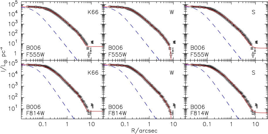
Figure 2.— Surface brightness profiles and model fits to one sample cluster B006, with the data of F555W and F814W band from top to bottom. The three panels in each line are fits to, from left to right: King model, Wilson model, and Sérsic model.

Most profiles of the sample clusters were well fitted by the models, except for several clusters with different reasons. There are one or several bright objects at the intermediate radii of B097D, GC9, and M091; the shape is very loose for DAO38; the signal-to-noise ratio (SNR) is low for B205; there are one or several bright objects near the outer region of B328, B331, and BH11; the images are not well resolved for B092, B101, B145, BH05, and NB39; several clusters (B324, B330, B333, B468, GC3, GC7, BH04, and BH29) are lack of a central brightness concentration, which may be candidates of “ring clusters”. The “ring clusters” have been reported in the Magellanic Clouds (MCs) and M33 (Mackey & Gilmore, 2003; Hill & Zaritsky, 2006; Werchan & Zaritsky, 2011; San Roman et al., 2012), with irregular profiles such as bumps and dips which may not be attributed to the random fluctuations due to a few luminous stars. The images of these “ring cluster” candidates in our sample are displayed in Figure 3. There are three clusters (B018, B114, and B268) showing bumps only in the luminosity profiles of the F814W, with the intrinsic color of $(V-I)_{0}=$ 0.95, 1.14, and 1.2, respectively. Some bright redder stars may locate at the intermediate radii of these clusters.

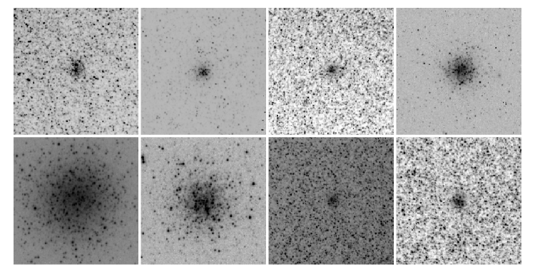
Figure 3.— Images (F555W or F606W) of eight “ring cluster” candidates. From the upper left, these are B324, B330, B333, B468, GC3, GC7, BH04, and BH29.

There are 15 clusters (B124, B127, B128, B148, B153, B167, B268, B331, BH05, BH12, M091, NB39, B064, B092, and B205) with high errors of $I_{\rm bkg}$. We checked the images carefully, and found that several reasons may account for those high errors: most of these clusters are not well resolved in the images; there are one or several bright objects in the intermediate and outer part of clusters B331 and M091; clusters B064 and B205 only have images in one band (F300W), of which the SNRs are low. We should notice that if the fitted background is too high, the tidal radius may be estimated smaller artificially. Only one band of observations can be derived for six clusters (B009, B020D, B064, B092, B101, B205), and none of the bands is close to $V$ band. So, we would not include the six objects in the following discussions.

We used the same method mentioned in Barmby et al. (2009) and Wang & Ma (2012) to transform the magnitudes from ACS and WFPC2 to $V$ on the vegamag scale (Holtzman et al., 1995; Sirianni et al., 2005). For clusters with available data of F555W or F606W band, we briefly used the extinction-corrected color $(V-I)_{0}$ or $(B-V)_{0}$ to do the transformations, while for clusters with no data of F555W or F606W band, we first transformed the ACS or WFPC2 magnitudes to $I$ magnitude using the color $(B-I)_{0}$, and then computed the $V$ magnitude using the color $(V-I)_{0}$. The $BVI$ magnitudes and the reddening values are listed in Table 1. We estimated a precision of $\pm 0.05$ mag in the transformation, which was propagated through the parameter estimates (Barmby et al., 2007; Wang & Ma, 2012).

The mass-to-light ratios ($M/L$ values), which were used to derive the dynamical parameters, were determined from the population-synthesis models of Bruzual & Charlot (2003), assuming a Chabrier (2003) initial mass function. The ages and metallicities used to computed $M/L$ values in $V$ band were derived as follows. An age of 13 Gyr with an uncertainty of $\pm 2$ Gyr was adopted for old clusters, while the derived average ages (in Section 2.2) were adopted for the young clusters. The metallicities with uncertainties are listed in Table 1. The errors for $M/L$ of old clusters include the uncertainties in age and metallicity, while for young clusters, we simply adopted $10\%$ in $M/L$ as the errors as Barmby et al. (2009) did.

The basic structures and various derived dynamical parameters of the best-fitting models for each cluster are listed in Table 5 to Table 7, with a description of each parameter/column at the end of each table (see for details of their calculation in Mclaughlin et al., 2008). The uncertainties of these parameters were estimated by calculating their variations in each model that yields $\chi^{2}$ within 1 of the global minimum for a cluster, while combined in quadrature with the uncertainties in $M/L$ for the parameters related to it (see Mclaughlin & van der Marel, 2005, for details).

3.3. Comparison with Previous Determinations

In this paper, we determined structural parameters for 79 clusters in M31 by comparing their surface brightness profiles with three structural models. In Figure 4, some estimated structural parameters for clusters in this paper were compared with those from previous studies (e.g., Barmby et al., 2002, 2007; Wang & Ma, 2012). Barmby et al. (2002, 2007) presented structural and dynamical parameters in $V$ band for 51 clusters in our sample, while Wang & Ma (2012) determined structures for 10 GCs using King model. So we used the results on the bandpass close to $V$ band (e.g., F475W, F555W, and F606W) and fitted by King model for comparison. It is not unexpected to see that most of our parameters are larger than the results from Barmby et al. (2002, 2007), since the isophotes flagged as “DEP” in this paper may not be excluded from the fitting process in Barmby et al. (2002), resulting in excessive weighting of the inner regions in the fits. In addition, the ellipticities presented by Barmby et al. (2002) were averaged over different filters for each cluster, while our results in Figure 4 were on the bandpass close to $V$ band. The cluster with the largest discrepancy of ellipticity is BH05, with an estimate of 0.19 by Barmby et al. (2002), and 0.55 in this paper. As discussed above, the image of BH05 is not well resolved, so it is difficult to derive accurate ellipticities and structural parameters. Barmby et al. (2007) also concluded that the shapes of outer parts of faint clusters are strongly affected by the galaxy background or low SNRs, leading to a difficult business to accurately measure the ellipticities. The largest scatter of the $R_{h}$ is B018, which is $\sim 5$ pc derived by Barmby et al. (2007), while $\sim 30$ pc in this paper. Although the PSFs and some calibration factors adopted here are slightly different from those of Wang & Ma (2012), the parameters derived here are in good agreement with their results.

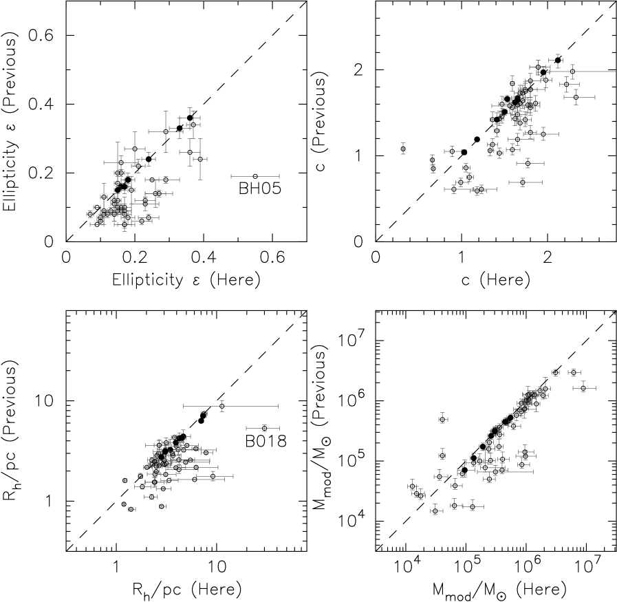
Figure 4.— Comparison of our newly obtained cluster structural parameters with previous measurements by Barmby et al. (2002, 2007) (open circles) and Wang & Ma (2012) (filled circles).

Strader et al. (2009, 2011) presented observed velocity dispersions for a number of GCs in M31 using new high-resolution spectra from MMT/Hectochelle. These authors estimated the $M/L$ values in $V$ band for clusters using the virial masses and luminosities, since the virial masses are the nominal estimates of the “global” mass of the system and are less sensitive to the accuracy of the King model fit (see Strader et al., 2009, 2011, for details). Here we estimated the $M/L$ values in $V$ band from population-synthesis models by giving their metallicities and various ages (Barmby et al., 2007, 2009). In Figure 5, We presented the comparison of some parameters derived by Barmby et al. (2007, 2009) and this paper with those from Strader et al. (2011). There is a large discrepancy between the $M/L$ values derived from the two methods, and most of the $M/L$ values from population-synthesis models are larger than those from observed velocity dispersions. The model masses from Barmby et al. (2007, 2009) and this paper are slightly larger than the virial masses from Strader et al. (2011), which were estimated using the half-mass radius and global velocity dispersion $\sigma_{\infty}$. The $\sigma_{p,\rm obs}$ values from Strader et al. (2011) were the central velocity dispersions estimated using the observed velocity dispersions by integrating a known King model over the fiber aperture, and are consistent with the predicted line-of-sight velocity dispersions at the cluster center from Barmby et al. (2007, 2009) and this paper. However, there are few young clusters with velocity dispersion measured by Strader et al. (2011), so more observation data and analysis are needed to check the conclusion of the comparisons.

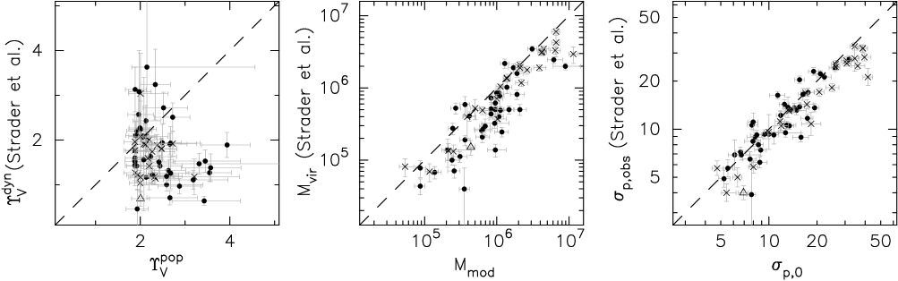
Figure 5.— Comparison of some dynamical parameters from Barmby et al. (2007) (crosses), Barmby et al. (2009) (triangles), and this paper (filled circles) with those from Strader et al. (2011).

Figure 6 plots the correlations of velocity dispersion and mass with $M/L$ for M31 clusters. The left two panels show these parameters of clusters from Strader et al. (2011), while the right two panels show those derived by King model from Barmby et al. (2007, 2009) and this paper. We can see that the $\sigma_{p,0}$ and $M_{\rm mod}$ from King-model fits show large dependence on the $M/L$. The old and young clusters show a distinct boundary of the $M/L$ values. There is no clear correlation for $M/L$ and $\sigma_{p,\rm obs}$ from Strader et al. (2011), while the decrease in $M/L$ toward lower masses is expected from dynamical evolution like evaporation, which is the steady loss of low-mass (high $M/L$) stars from the cluster driven by relaxation (Portegies et al., 2010). Considering the sensitive dependence on $M/L$ of $\sigma_{p,0}$, in the following discussion of the correlations of velocity dispersion with ellipticity and [Fe/H], we decided to use the $\sigma_{p,\rm obs}$ values from Strader et al. (2011) for clusters in Barmby et al. (2007, 2009) and this paper.

Figure 6.— Correlations of velocity dispersion and mass with $M/L$ in $V$ band. Left panels show clusters from Strader et al. (2011) (asterisks) while right panels show clusters from Barmby et al. (2007) (crosses), Barmby et al. (2009) (triangles), and this paper (filled circles).

3.4. Comparison of Three Model Fittings

In order to determine which model can describe the structure of clusters best, Mclaughlin & van der Marel (2005) and Mclaughlin et al. (2008) defined a relative $\chi^{2}$ index, which compares the $\chi^{2}$ of the best fit of an “alternate” model with the $\chi^{2}$ of the best fit of King model,

$$\Delta=(\chi^{2}_{\rm alternate}-\chi^{2}_{\rm K66})/(\chi^{2}_{\rm alternate}+\chi^{2}_{\rm K66}).$$ (10)

It is evident that the “alternate” model is a better fit than King model if $\Delta$ is negative, while King model is a better fit if $\Delta$ is positive.

Figure 7 shows the relative quality of fit, $\Delta$ for Wilson- and Sérsic-model fits versus King-model fits for the sample clusters in this paper. The $\Delta$ values are plotted as a function of age and some structures, including the half-light radius $R_{h}$, the total model luminosity $L_{\rm mod}$, and the surface brightness over the half-light radius in the $V$ band $<\mu_{V}>_{h}$. The circles refer to clusters with $R_{\rm last}\geq 5R_{h}$, while triangles present those with $R_{\rm last}<5R_{h}$, where $R_{\rm last}$ is the most large radius for the available observation data. It can be seen that most clusters with $R_{\rm last}<5R_{h}$ are those having fainter luminosity $L_{\rm mod}$ or surface brightness $<\mu_{V}>_{h}$. Mclaughlin & van der Marel (2005) presented that the fitting data out to $R_{\rm last}\geq 5R_{h}$ can effectively constrain the model fitting to the outer regions, which are essential to determine which structural model best describes the clusters. However, when $R_{\rm last}$ is small ($<5R_{h}$), few data are available at large cluster radii, and the fitting are mostly dependent on the inner part. So, these clusters cannot be used to determine a preference of one model or the other. Similarly, we cannot conclude that these clusters are well fitted by both two models even $\Delta$ for them are small. Mclaughlin et al. (2008) determined a catalogue of structural and dynamical parameters for GCs in NGC 5128 using the three models, and showed that the bright clusters ($L_{\rm mod}>10^{5}L_{\odot}$) are better fitted by Wilson model and Sérsic model, indicating that the halos of clusters in NGC 5128 are more extended than what King model describes. There is no evident correlation of $\Delta$ with $L_{\rm mod}$ and $<\mu_{V}>_{h}$ for clusters in this paper. Several studies (Elson, Fall & Freeman, 1987; San Roman et al., 2012) showed that young clusters in the Large Magellanic Cloud (LMC) and M33 do not appear to be tidally truncated and seem to be better fitted by power-law profiles than King models, while old clusters show no clear differences between the qualities of the fittings. However, there is no correlation of $\Delta$ with age in Figure 7. We should notice that there are only six young clusters in our sample, and 13 clusters with no ages estimated in previous studies are assumed to be 13 Gyr. A large sample of young star clusters with precise age estimates are needed for the study on correlation of $\Delta$ with age. However, we do see that the King- and Wilson-model fits are better than the Sérsic-model fits. We concluded that clusters in M31 can be well fitted by both King model and Wilson model (also reported in Barmby et al., 2007, 2009).

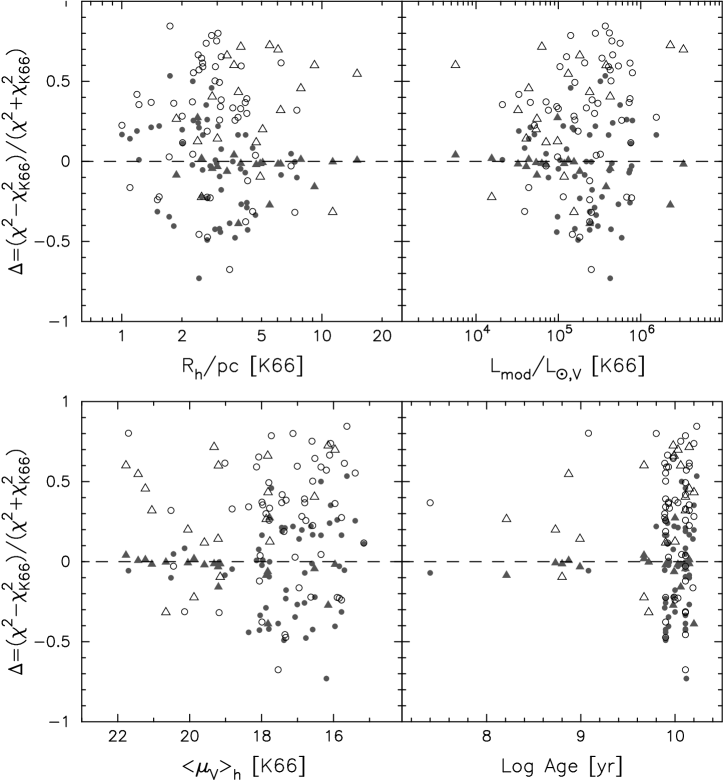
Figure 7.— Relative quality of fit for Wilson and Sérsic models (grey and open circles refer to the clusters with $R_{\rm last}\geq 5R_{h}$, while grey and open triangles the clusters with $R_{\rm last}<5R_{h}$) versus King models for the sample clusters in this paper.

Figure 8 compares the relative quality of fit, $\Delta$ values with a number of structure parameters ($R_{c}$, $R_{h}$, $\mu_{V,0}$, $L_{\rm mod}$, $\sigma_{p,0}$, and $E_{b}$) for the sample clusters in this paper. The grey and open circles show the physical properties of clusters with $R_{\rm last}\geq 5R_{h}$ derived from Wilson- and Sérsic-model fits comparing to King-model fits, respectively. The triangles refer to clusters with $R_{\rm last}<5R_{h}$. There are some clusters with comparable $\chi^{2}$, but large discrepancy of $R_{h}$ and $L_{\rm mod}$ values for King- and Wilson-model fits. We can see that most of these clusters have $R_{\rm last}<5R_{h}$. As discussed above, the few constrain of the fitting to outer regions results in much different extrapolations of models, and it is hard to determine which model does the correct fitting in those cases (Mclaughlin & van der Marel, 2005). Most parameters derived from Wilson model are slightly larger than those from King model, while parameters derived by Sérsic model are smaller than those from King model, especially for $R_{c}$, $\sigma_{p,0}$, and $E_{b}$. Barmby et al. (2007) concluded that rather than an intrinsic difference between clusters in M31 and other galaxies, the preference for King models over Wilson models for M31 clusters is due to some subtle features of the observations.

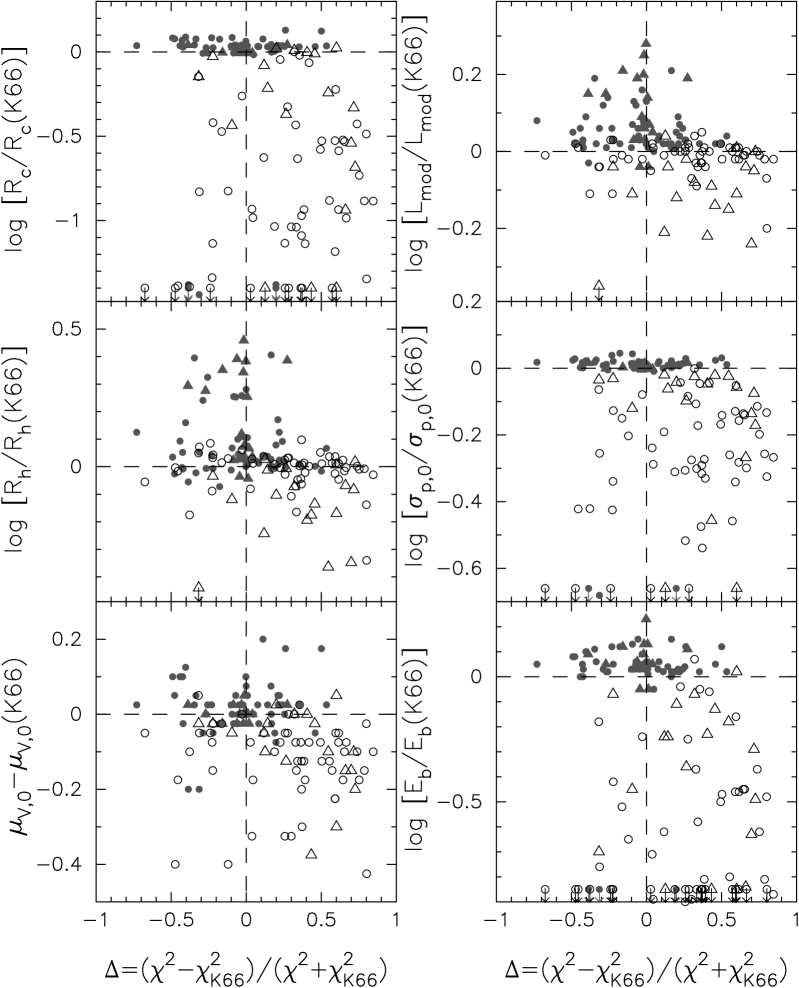
Figure 8.— Comparison of some parameters for Wilson and Sérsic models versus King models for the sample clusters in this paper, including the projected core radius $R_{c}$, the projected half-light radius $R_{h}$, the central surface brightness in the $V$ band $\mu_{V,0}$, the total model luminosity $L_{\rm mod}$, the predicted central line-of-sight velocity dispersion $\sigma_{p,0}$, and the global binding energy $E_{b}$. Symbols are as in Fig. 7.

4. DISCUSSION

We combined the newly derived parameters here with those derived by King-model fits for M31 young massive clusters (YMCs) (Barmby et al., 2009), M31 globulars (Barmby et al., 2007), M31 extended clusters (ECs) (Huxor et al., 2011), and MW globulars (Mclaughlin & van der Marel, 2005) to construct a large sample to look into the correlations between the parameters. The ellipticities and galactocentric distances for the MW GCs are from Harris (1996) (2010 edition). The parameters used in the following discussion for M31 GCs (Barmby et al., 2007) are those derived on the bandpass close to $V$ band (e.g., F555W and F606W), while the data from bluer filters are preferred for the YMCs in Barmby et al. (2009). The metallicities for most young clusters in Barmby et al. (2009) were assumed to be solar metallicity, while metallicities from Perina et al. (2010) were adopted for some older clusters (B083, B222, B347, B374, and NB16). Huxor et al. (2011) derived structure parameters of 13 ECs, including the core radius, half-light radius, tidal radius, and the central surface brightness in magnitude. The metallicities of 4 ECs (HEC4, HEC5, HEC7 and HEC12) were determined by Mackey et al. (2006), and the integrated cluster masses for them were derived here using the absolute magnitudes and $M/L$ values in $V$ band from population-synthesis models (see Wang & Ma, 2012, for the details).

4.1. Galactocentric Distance

Figure 9 shows structural parameters as a function of galactocentric distance $R_{\rm gc}$ for the new large sample clusters in M31 and the MW. Some global trends can be seen. Both $R_{h}$ and $r_{t}$ increase with the $R_{\rm gc}$ as expected, although the trend is largely driven by the ECs from Huxor et al. (2011). The star clusters with large $R_{\rm gc}$ can keep more stars with weaker tides relatively to those located at bulge and disk. Georgiev et al. (2009) explained that the $R_{h}$ and $r_{t}$ of the clusters in the halo of galaxies, which may be accreted into the galaxies from dwarf galaxies, can expand due to the change from strong to a weaker tidal field. Barmby et al. (2002) concluded that the correlation of $R_{h}$ with $R_{\rm gc}$ reflects physical formation conditions as suggested by van den Bergh (1991) for GCs in the MW. However, Strader et al. (2012) found that no clear correlation between $R_{h}$ and $R_{\rm gc}$ exists beyond $R_{\rm gc}\sim 15$ kpc for GCs in NGC 4649, and they suggested that the sizes of GCs are not generically set by tidal limitation. It can be seen that there are no compact clusters at large radii ($R_{\rm gc}>40$ kpc) in the MW, while in M31, there is a bimodality in the size distribution of GCs at large radii (also reported in Huxor et al., 2011; Wang & Ma, 2012). It is interesting that there are few GCs having $R_{h}$ in the range from 8 to 15 pc at large radii ($R_{\rm gc}>40$ kpc) in M31. There are three clusters (B124, B127, and NB39) with large $R_{h}$ and $r_{t}$ at small $R_{\rm gc}$, leading to more diffuse trends. However, the total model masses for them are $10^{6.95}$, $10^{6.79}$, and $10^{5.93}M_{\odot}$, respectively, meaning that they are massive clusters. It is not unexpected that these massive clusters can contain more stars than other clusters, although they are at small $R_{\rm gc}$. The luminosities of clusters decrease with increasing $R_{\rm gc}$, implying that either strong dynamical friction drives predominantly more massive GCs inwards, or massive GCs may favor to form in the nuclear regions of galaxies with the higher pressure and density (Georgiev et al., 2009). However, the lack of faint clusters with small galactocentric distance may be due to selection effects, since these clusters are difficult to detect against the bright background near M31 center, which is also reported by Barmby et al. (2007) using the correlation of central surface brightness with galactocentric distance. The metallicities of clusters decrease with increasing $R_{\rm gc}$, indicating that metal-rich clusters are typically located at smaller galactocentric radii than metal-poor ones, although with large scatter. van den Bergh (1991) found that metal-rich clusters ([Fe/H]$\geq-0.8$) in M31 seem to form in a rotating disk extending to $R_{\rm gc}\simeq 5$ kpc. The metal-rich GCs may have undergone accelerated internal evolution due to strong tidal shocks (Strader et al., 2011) from both bulge and disk passages. There are two matal-poor clusters (B114, B324) at small $R_{\rm gc}$, which are at the bottom-left in the [Fe/H]-$R_{\rm gc}$ panel. The diffuse distribution of these parameters vs. $R_{\rm gc}$ may be caused by the different galactocentric distance used, which is true three-dimensional distances for Galactic GCs while projected radii for M31 clusters.

Figure 9.— Structural parameters vs. galactocentric distance $R_{\rm gc}$. The filled circles are the sample clusters in M31 (this paper), the open circles are Galactic GCs (Mclaughlin & van der Marel, 2005), the crosses are M31 GCs (Barmby et al., 2007), the open triangles are M31 YMCs (Barmby et al., 2009), and the open stars are M31 ECs (Huxor et al., 2011).

4.2. Ellipticity

Figure 10.— Ellipticity as a function of galactocentric distance, metallicity, the observed velocity dispersion, and structure parameters. Symbols are as in Fig. 9.

Figure 10 shows the distribution of ellipticity with galactocentric distance, metallicity, and some structure parameters for clusters in the MW and M31, which may show clues to the primary factor for the elongation of clusters: rotation and velocity anisotropy, cluster mergers, “remnant elongation”, and galaxy tides (Larsen et al., 2001; Barmby et al., 2007). Geyer et al. (2009) presented that the tidal forces can only distort a cluster’s outer region, while the elongation of the inner parts are due to its own gravitational potential and the total orbital angular momentum.

1) Rotation and velocity anisotropy. Cluster rotation is the generally accepted explanation for cluster flattening (Davoust & Prugniel, 1990). Dynamical models show that internal relaxation coupled to the external tides will drive a cluster toward a rounder shape over several relaxation times (see Harris et al., 2002, and references therein). Barmby et al. (2002) presented that more compact clusters which experience more relaxation processes, and clusters with larger velocity dispersions which rotate more slowly, should be rounder. Barmby et al. (2007) presented that dynamical evolution could reduce the initial flattening caused by rotation or velocity anisotropy, indicating that more evolved clusters would be rounder. In order to check these predictions, we show the correlations of $r_{0}$, $c$, the observed velocity dispersion $\sigma_{p,\rm obs}$, and $t_{r,h}$ with the ellipticity. The observed velocity dispersion $\sigma_{p,\rm obs}$ for M31 clusters are from Strader et al. (2011), while $\sigma_{p,\rm obs}$ for clusters in the MW are from Mclaughlin & van der Marel (2005). All the $\sigma_{p,\rm obs}$ have been extrapolated to their central values with an aperture of 0. There is no clear correlation of ellipticity with these parameters. However, we do see that more compact clusters–smaller $r_{0}$ and larger $c$–are more rounder, which is consistent with previous studies (Barmby et al., 2002).

2) Cluster mergers and “remnant elongation”. van den Bergh & Morbey (1984) presented that ellipticity correlates strongly with luminosity for clusters in LMC: more luminous clusters are more flattened, while van den Bergh (1996) presented that the most flattened GCs in both the MW and M31 are also brightest. This may be explained by the cluster mergers and “remnant elongation”, which is from some clusters’ former lives as dwarf galaxy nuclei. So, the larger ellipticities for clusters located at large galactocentric radii of M31 may be related to the merger or accretion history that M31 has experienced (e.g. Bekki, 2010; Mackey et al., 2010; Huxor et al., 2011). However, no clear correlation of ellipticity with luminosity can be seen.

3) Galaxy tides. A strong tidal field might rapidly destroy the velocity anisotropies, and force an initially triaxial, rapidly rotating elliptical GC to a more isotropic distribution and spherical shape, while weak tidal fields are unable to change the initial shapes of GCs (Goodwin, 1997). It seems plausible that clusters located at different galactocentric radii or different galaxies have various distributions of ellipticities, due to the diverse galaxy tides. Harris et al. (2002) and Barmby et al. (2007) found the distributions of ellipticities for M31 and NGC 5128 are very similar, but differ from the MW distribution, which has few very round clusters. No clear correlation of ellipticity with $R_{\rm gc}$ can be seen for clusters in these galaxies (also see Barmby et al., 2007). However, the innermost clusters are slightly more spherical (Barmby et al., 2002), which may due to the strong tidal field near galaxy center that reduces ellipticities of them. Some clusters located at large projected radii of M31 do have larger ellipticities than most GCs in M31 and the MW, which may be caused by galaxy tides coming from satellite galaxies (Wang & Ma, 2012).

San Roman et al. (2012) summarized the orientation of a large sample of clusters in M33 and found that the distribution of PAs shows a strong peak at $-55^{\circ}$, which is close to the direction towards M31. These authors suggested that the elongation of clusters in M33 may be attributed to the tidal forces of M31, considering that a recent encounter between M33 and M31 (McConnachie et al., 2009; Putman et al., 2009; San Roman et al., 2010; Bernard et al., 2012) may have led to significant effects on the properties of M33 disk. Figure 11 depicts the distribution of PAs of star clusters in this paper and 34 clusters from Barmby et al. (2007), which were not included in Barmby et al. (2002). No clear trend is present in the orientation vectors towards M33, although a small peak at $-60^{\circ}$ does exist in the distribution of the PAs. Here we concluded that the elongation of clusters seems to be due to various factors (Barmby et al., 2007).

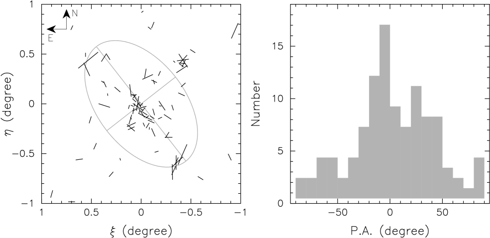
Figure 11.— ($Left~{}panel$) Cluster elongations and orientations shown with respect to M31. The vector sizes are correlated with the ellipticities. The ellipse has a radius of 10 kpc and is flattened to $b/a=0.6$. ($Right~{}panel$) Distribution of the P.A.s of star clusters in M31.

4.3. Metallicity

Figure 12 plots structural parameters as a function of [Fe/H] for the new large sample clusters in M31 and the MW. The trends of the parameters with [Fe/H] nearly disappear when we add the data for the M31 YMCs, which were fitted with solar metallicities (Barmby et al., 2009). However, we noticed that the metallicities for most of these YMCs obtained by Kang et al. (2012) are poorer than [Fe/H]$=-1.1$. If we do not consider the YMCs in Barmby et al. (2009), it is evident that the metal-rich clusters have smaller average values of $R_{h}$ than those of metal-poor ones (Larsen et al., 2001; Barmby et al., 2002). Strader et al. (2012) presented that the sizes of metal-rich GCs are smaller than the metal-poor ones in NGC 4649, which is a massive elliptical galaxy in the Virgo galaxy cluster. These authors explained that as an intrinsic size difference rather than projection effects. Sippel et al. (2012) carried out N-body simulations of metallicity effects on cluster evolution, and found that there is no evident difference for the half-mass radii of metal-rich and metal-poor cluster models. So, they explained that metal-rich and metal-poor clusters have similar structures, while metallicity effects combined with dynamical effects such as mass segregation produce a larger difference of the half-light radii. Barmby et al. (2007) also found that $R_{h}$ decreases with increased metallicity for GCs in the MW, the MCs, Fornax dwarf spheroidal, and M31, except for GCs in NGC 5128. An evident feature is that these four ECs are all metal-poor and have large $R_{h}$. No clear correlation of model luminosity $L_{\rm mod}$ with [Fe/H] is present, but we do see that the metal-rich clusters tend to be more luminous. Both the observed velocity dispersion $\sigma_{p,\rm obs}$ and central “escape” velocity $\nu_{\rm esc,0}$ increase with metallicity. Georgiev et al. (2009) presented that the higher $\nu_{\rm esc}$ of more metal-rich clusters in the observation may reflect the metallicity dependence of the terminal velocities of the stellar winds, since the $\nu_{\rm esc}$ of a metal-rich cluster should be higher to retain the fast stellar winds.

Figure 12.— Structural parameters and the observed velocity dispersion as a function of [Fe/H]. Symbols are as in Fig. 9.

4.4. Core-collapsed Clusters

Core-collapsed clusters in general show a power-law slope in the central surface brightness profiles, which can be better fitted by a power-law model than King model (Barmby et al., 2002). Noyola & Gebhardt (2006) presented that the process of core collapse can be divided into two stages. In the first stage, stars are driven to the halo of the cluster due to close encounters. Stellar evaporation occurs and the core contracts due to energy conservation. In the second stage, the low-mass stars are scattered to high velocities and escape to the halo, while the high-mass stars sink to the core due to energy equipartition. The increasing core density also increases the interaction rate of the binaries and single stars, which can generate energy in the core, reverse the contraction process, and produce an expansion. After a long time, the core shrinks again, and the process repeats. M15, which has a central cusp, may be at an intermediate state between the extremes of collapse and expansion (Dull et al., 1997). Chatterjee et al. (2012) presented that the core-collapsed clusters are those that have reached or are about to reach the “binary burning” stage, while the non core-collapsed clusters are still contracting under two-body relaxation. Trager et al. (1995) presented a catalogue of surface brightness profiles of 125 Galactic GCs, and classified 16% of their sample as core-collapsed clusters and 6% as core-collapsed candidates. Mclaughlin et al. (2008) noticed that a number of clusters (more than half of their sample) in NGC 5128 have the index $n>2$ derived from Sérsic model, indicating that these clusters have strongly peaked central density profiles. These authors explained that the PSF may flatten the models, and then the cuspy central density profiles are shown relatively. Noyola & Gebhardt (2006) presented that Galactic clusters with steep cusps are all close to the center of the Galaxy, indicating that an increased incidence of tidal shocking (Gnedin et al., 1999) may accelerate the core collapse process. Barmby et al. (2002) also concluded that most of the M31 core-collapsed candidates are within 2 kpc of the center of M31.

Figure 13 shows the distributions of galactocentric distance, and some structure parameters derived from Sérsic-model fitting for clusters in this paper and M31 GCs in Barmby et al. (2007). There are 25 clusters bested fitted by Sérsic model ($\chi^{2}_{\rm S}<\chi^{2}_{\rm K66}$ and $\chi^{2}_{\rm S}<\chi^{2}_{\rm W}$), and 11 of them have $n>2$, indicating that they have cuspy central density profiles. We assumed these 11 clusters to be possible core-collapsed clusters. In fact, the clusters with $n>2$ do have smaller $R_{c}$ and larger $R_{h}/R_{c}$ than their counterparts with $n<2$. Barmby et al. (2002) presented several clusters (B011, B064, B092, B123, B145, B231, B268, B343, and BH18) as core-collapsed candidates in M31. However, most of these clusters are best fitted by King model or Wilson model in this paper except B145 and B343. We checked the images of these clusters and found that the images of B123, B231, and B268 are not fully resolved, while the SNRs of images for B064 and B092 are low. Actually, the discrimination between the core-collapsed clusters and the “King model clusters” (Meylan & Heggie, 1997) may often become unclear for several reasons: (1) statistical noise due to some unresolved bright stars in the cores of clusters; (2) the similarity between the high-concentration King-model and power-law profiles (see Meylan & Heggie, 1997, for details). B145 is best fitted by Sérsic model in this paper, but $n=1.5$. The cluster B343 shows a cuspy density profile in the center, and has been classified as a core-collapsed cluster (Bendinelli et al., 1993; Grillmair et al., 1996). We also find a better fitting by Sérsic model for it with $n=3.35$. The distribution of core-collapsed cluster candidates is not constrained to the center of M31. There are only two out of the 11 clusters with $R_{\rm gc}<2$ kpc, while four ones with $R_{\rm gc}>15$ kpc.

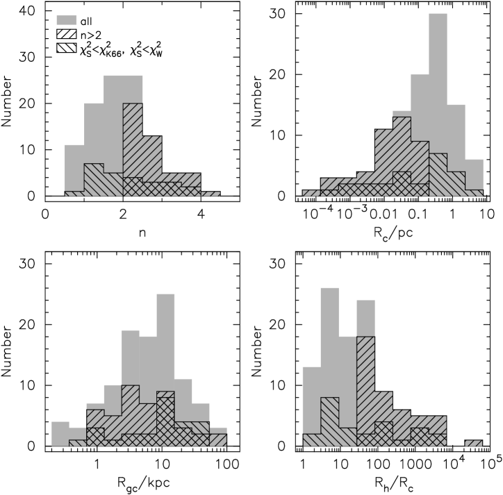
Figure 13.— The distributions of the galactocentric distance and several structure parameters derived from Sérsic-model fitting for clusters in this paper and M31 GCs in Barmby et al. (2007).

4.5. The Fundamental Plane

Figure 14.— Evidence of an FP of the cluster parameters, which is defined in terms of central velocity dispersion $\sigma_{p,0}$, radius $R_{c}$ or $R_{h}$, and surface mass density $<\Sigma>_{0}$ or $<\Sigma>_{h}$. Symbols are as in Fig. 9.

It has been widely noticed that GCs do not occupy the full four-dimensional parameter space (concentration $c$, scale radius $r_{0}$, central surface brightness $\mu_{V,0}$, and central $M/L$ or velocity dispersion $\sigma_{0}$) instead locate in a remarkably narrow “fundamental plane” (FP). It is interesting to learn which of the structural and dynamical properties are either universal or dependent on characteristics of their parent galaxies (Meylan & Heggie, 1997). Djorgovski & Meylan (1994) explored some tight correlations between various properties using a large sample of Galactic clusters, and Djorgovski (1995) defined an FP for GCs in terms of velocity dispersion, radius, and surface brightness. Saito (1979) investigated the mass-binding energy relationship for a few GCs and ellipticals, while McLaughlin (2000) defined an FP using the binding energy and luminosity, which is formally different from that of Djorgovski (1995). Harris et al. (2002) found that the NGC 5128 GCs describe a relation between binding energy and luminosity tighter than in the MW. Here we show the two forms of the FP for the new large sample clusters in the MW and M31.

Figure 14 shows the mass-density-based FP relations. The left two panels show the correlations of the properties derived with the $M/L$ values from the velocity dispersions (Strader et al., 2011), using King model and the same fitting process in this paper (Section 3), while the right two panels show the correlations of the properties derived with the $M/L$ values from population-synthesis models. Barmby et al. (2009) presented the surface-brightness-based FP relations and found a large offset between the young M31 clusters and old clusters. They explained that as a result from lower $M/L$ values for the young clusters in M31. It is obvious that the velocity dispersion, characteristic radii, and surface density for these clusters show tight relations, both on the core and half-light scales. The exist of FP for clusters strongly reflects some universal physical conditions and processes of cluster formation.

Figure 15 shows the correlation of binding energy with the total model mass. The left panel shows the $M_{\rm mod}$ and $E_{b}$ derived with the $M/L$ from the directly observed velocity dispersions (Strader et al., 2011), using King model and the same fitting process in this paper (Section 3), while the right panel shows those properties derived with the $M/L$ from population-synthesis models. All the clusters locate in a remarkably tight region although in the widely different galaxy environments, which is consistent with the previous studies (Barmby et al., 2007, 2009). Barmby et al. (2007) concluded that the scatter around this relation is so small that the structures of star clusters may be far simpler than those scenarios derived from theoretical arguments.

Figure 15.— Evidence of an FP of the cluster parameters, which is defined in terms of binding energy $E_{b}$ and the total model mass $M_{\rm mod}$. Symbols are as in Fig. 9.

5. SUMMARY

High-resolution imaging can be derived from HST observations for M31 star clusters. In this paper, we presented surface brightness profiles for 79 clusters, which were selected from Barmby et al. (2002) and Mackey et al. (2007). Structural and dynamical parameters were derived by fitting the profiles to three different models, including King model, Wilson model, and Sérsic model. We found that in the majority of cases, King models fit the M31 clusters as well as Wilson models, and better than Sérsic models.

We discussed the properties of the sample GCs here combined with GCs in the MW (Mclaughlin & van der Marel, 2005) and clusters in M31 (Barmby et al., 2007, 2009; Huxor et al., 2011). In general, the properties of the M31 and the Galactic clusters fall in the same regions of parameter spaces. There is a bimodality in the size distribution of M31 clusters at large radii, which is different from their Galactic counterparts. There are 11 clusters in M31 best fitted by Sérsic models with index $n>2$, meaning that they have cuspy central density profiles, which are classified as core-collapsed cluster candidates. We investigated two forms of the FP, including the correlation of velocity dispersion, radius, and surface density, and the correlation of binding energy with the total model mass. The tight correlations of cluster properties indicate a tight FP for clusters, regardless of their host environments, which is consistent with previous studies (Barmby et al., 2007, 2009). In addition, the tightness of the relations for the internal properties indicates some physical conditions and processes of cluster formation in different galaxies.

Table 1Integrated measurements for 79 sample clusters in M31.

Name	$\epsilon^{a}$	$\theta^{a}$	$\epsilon^{b}$	$\theta^{b}$	$B$	$V$	$I$	$R_{\rm gc}$	$E(B-V)$	${\rm[Fe/H]}$	${\rm Age}$
		(deg E of N)		(deg E of N)	(Vegamag)	(Vegamag)	(Vegamag)	(kpc)			(Gyr)
(1)	(2)	(3)	(4)	(5)	(6)	(7)	(8)	(9)	(10)	(11)	(12)
B006	$0.14\pm 0.01$	$-40\pm 8$	$0.24\pm 0.02$	$-45\pm 8$	16.49	15.50	14.33	6.43	0.11	$-0.59\pm 0.41$	13.25
B011	$0.12\pm 0.01$	$21\pm 8$	$0.15\pm 0.01$	$32\pm 7$	17.46	16.58	15.56	7.73	0.09	$-1.71\pm 0.24$	15.85
B012	$0.17\pm 0.02$	$24\pm 8$	$0.14\pm 0.01$	$18\pm 7$	15.86	15.09	14.03	5.78	0.11	$-1.91\pm 0.21$	8.00
B018	$0.19\pm 0.01$	$-9\pm 5$	$0.15\pm 0.02$	$-5\pm 8$	18.37	17.53	16.38	9.31	0.20	$-0.77\pm 0.39$	1.20
B027	$0.18\pm 0.02$	$11\pm 7$	$0.16\pm 0.03$	$-12\pm 9$	16.49	15.56	14.41	6.02	0.19	$-1.64\pm 0.16$	15.75
B030	$0.16\pm 0.01$	$-12\pm 12$	$0.13\pm 0.01$	$-37\pm 6$	18.75	17.39	15.68	5.66	0.57	$-0.14\pm 0.26$	9.62
B045	$0.12\pm 0.01$	$-13\pm 6$	$0.16\pm 0.02$	$-13\pm 7$	16.72	15.78	14.51	4.90	0.18	$-1.01\pm 0.50$	11.40
B058	$0.09\pm 0.01$	$-27\pm 8$	$0.11\pm 0.01$	$-36\pm 9$	15.81	14.97	13.87	6.96	0.12	$-1.02\pm 0.21$	8.01
B068	$0.21\pm 0.02$	$31\pm 3$	$0.18\pm 0.02$	$37\pm 4$	17.60	16.39	14.84	4.32	0.42	$-0.41\pm 0.17$	7.90
B070	$0.12\pm 0.01$	$1\pm 10$	$0.16\pm 0.02$	$-24\pm 11$	17.61	16.76	15.72	2.46	0.12	$-1.42\pm 0.43$	8.75

Table 2Calibration Data for HST images.

Filter	Pivot $\lambda$	$R_{\lambda}^{a}$	Zeropointb	$M_{\odot}^{c}$	Conversion Factord	Coefficiente
	(Å)
(1)	(2)	(3)	(4)	(5)	(6)	(7)
Calibration Data for ACS/WFC images
F435W	4318.9	4.20	25.779	5.459	3.1693	27.031
F475W	4746.9	3.72	26.168	5.167	1.6926	26.739
F555W	5361.0	3.19	25.724	4.820	1.8508	26.392
F606W	5921.1	2.85	26.398	4.611	0.8207	26.183
F814W	8057.0	1.83	25.501	4.066	1.1349	25.638
Calibration Data for WFPC2 images
F300W	2986.8	5.66	21.448	6.061	297.9614	27.633
F450W	4555.4	3.93	24.046	5.263	13.0545	26.835
F555W	5439.0	3.14	24.596	4.804	5.1542	26.376
F606W	5996.8	2.81	24.957	4.581	3.0100	26.153
F814W	8012.2	1.85	23.677	4.074	6.1342	25.646

Table 3The intensity profiles for 79 sample clusters in M31.

Name	Detector	Filter	$R$	$I$	Uncertainty	Flag
			(arcsec)	($L_{\odot}$ pc-2)	($L_{\odot}$ pc-2)
(1)	(2)	(3)	(4)	(5)	(6)	(7)
B006	WFPC2/PC	F555W	0.0234	44001.773	155.603	OK
	WFPC2/PC	F555W	0.0258	43776.562	171.971	DEP
	WFPC2/PC	F555W	0.0284	43528.629	188.743	DEP
	WFPC2/PC	F555W	0.0312	43258.270	206.935	DEP
	WFPC2/PC	F555W	0.0343	42964.875	227.137	DEP
	WFPC2/PC	F555W	0.0378	42647.070	249.659	DEP
	WFPC2/PC	F555W	0.0415	42303.609	274.847	DEP
	WFPC2/PC	F555W	0.0457	41919.195	299.011	DEP
	WFPC2/PC	F555W	0.0503	41381.914	308.833	OK
	WFPC2/PC	F555W	0.0553	40666.176	309.009	DEP
	WFPC2/PC	F555W	0.0608	39884.902	322.641	DEP
	WFPC2/PC	F555W	0.0669	38966.234	328.825	DEP
	WFPC2/PC	F555W	0.0736	37925.949	316.808	OK

Table 4Coefficients for the PSF models.

Detector	Filter	$r_{0}$	$\alpha$	$\beta$
		(arcsec)
(1)	(2)	(3)	(4)	(5)
ACS/WFC	F435W	0.068	3	3.80
	F475W	0.064	3	3.60
	F555W	0.057	3	3.39
	F606W	0.053	3	3.14
	F814W	0.056	3	3.05
WFPC2/WFC	F300W	0.076	2	5.05
	F450W	0.073	2	4.89
	F555W	0.064	2	4.35
	F606W	0.059	2	4.11
	F814W	0.051	2	3.71
WFPC2/PC	F300W	0.051	2	3.76
	F555W	0.045	2	3.10
	F606W	0.045	2	2.96
	F814W	0.059	2	3.18

Table 5Basic parameters of 79 sample clusters in M31.

Name	Detector	Band	$N_{\rm pts}$a	Model	$\chi_{\rm min}^{2}$b	$I_{\rm bkg}$c	$W_{0}$d	$c/n$e	$\mu_{0}$f	$\log r_{0}$g	$\log r_{0}$h
						($L_{\odot}$ pc-2)			${\rm(mag~{}arcsec^{-2})}$	(arcsec)	(pc)
(1)	(2)	(3)	(4)	(5)	(6)	(7)	(8)	(9)	(10)	(11)	(12)
B006	WFPC2/PC	555	49	K66	35.44	$5.10\pm 1.54$	$7.90^{+0.14}_{-0.21}$	$1.80^{+0.04}_{-0.07}$	$14.43^{+0.04}_{-0.07}$	$-0.900^{+0.012}_{-0.014}$	$-0.320^{+0.012}_{-0.014}$
			49	W	5.53	$-8.30\pm 0.92$	$7.60^{+0.04}_{-0.06}$	$2.86^{+0.03}_{-0.05}$	$14.44^{+0.01}_{-0.03}$	$-0.850^{+0.009}_{-0.007}$	$-0.270^{+0.009}_{-0.007}$
			49	S	130.08	$3.50\pm 2.56$	$\ldots$	$2.60^{+0.06}_{-0.04}$	$14.28^{+0.12}_{-0.08}$	$-2.400^{+0.032}_{-0.050}$	$-1.820^{+0.032}_{-0.050}$
B006	WFPC2/PC	814	49	K66	14.97	$6.00\pm 3.36$	$8.20^{+0.29}_{-0.22}$	$1.89^{+0.09}_{-0.07}$	$13.35^{+0.08}_{-0.08}$	$-0.950^{+0.013}_{-0.026}$	$-0.370^{+0.013}_{-0.026}$
			49	W	1.88	$-9.90\pm 2.25$	$7.60^{+0.10}_{-0.07}$	$2.86^{+0.09}_{-0.06}$	$13.39^{+0.04}_{-0.02}$	$-0.850^{+0.006}_{-0.007}$	$-0.270^{+0.006}_{-0.007}$
			49	S	32.24	$4.40\pm 3.68$	$\ldots$	$2.65^{+0.06}_{-0.06}$	$16.44^{+0.50}_{-0.50}$	$-2.450^{+0.038}_{-0.039}$	$-1.870^{+0.038}_{-0.039}$

Table 6Derived structural and photometric parameters of 79 sample clusters in M31.

Name	Detector	Band	Model	$\log r_{\rm tid}$a	$\log R_{c}$b	$\log R_{h}$c	$\log R_{h}/R_{c}$d	$\log I_{\rm 0}$e	$\log j_{\rm 0}$f	$\log L_{V}$g	$V_{\rm tot}$h	$\log I_{h}$i	$<\mu_{V}>_{h}$j
				(pc)	(pc)	(pc)		($L_{\odot,V}$ pc-2)	($L_{\odot,V}$ pc-3)	($L_{\odot,V}$)	(mag)	($L_{\odot,V}$ pc-2)	${\rm(mag~{}arcsec^{-2})}$
(1)	(2)	(3)	(4)	(5)	(6)	(7)	(8)	(9)	(10)	(11)	(12)	(13)	(14)
B006	WFPC2/PC	555	K66	$1.48^{+0.05}_{-0.06}$	$-0.333^{+0.010}_{-0.013}$	$0.386^{+0.058}_{-0.077}$	$0.719^{+0.071}_{-0.087}$	$4.79^{+0.03}_{-0.03}$	$4.81^{+0.05}_{-0.04}$	$5.63^{+0.02}_{-0.03}$	$15.18^{+0.07}_{-0.06}$	$4.06^{+0.12}_{-0.09}$	$16.20^{+0.23}_{-0.31}$
			W	$2.59^{+0.04}_{-0.04}$	$-0.295^{+0.008}_{-0.007}$	$0.511^{+0.046}_{-0.086}$	$0.807^{+0.053}_{-0.093}$	$4.78^{+0.02}_{-0.02}$	$4.77^{+0.03}_{-0.03}$	$5.71^{+0.02}_{-0.03}$	$14.98^{+0.08}_{-0.06}$	$3.89^{+0.14}_{-0.07}$	$16.63^{+0.17}_{-0.35}$
			S	$\infty$	$-1.820^{+0.032}_{-0.050}$	$0.399^{+0.126}_{-0.121}$	$2.218^{+0.176}_{-0.153}$	$4.85^{+0.04}_{-0.05}$	$5.49^{+0.08}_{-0.08}$	$5.63^{+0.07}_{-0.07}$	$15.18^{+0.16}_{-0.18}$	$4.04^{+0.18}_{-0.18}$	$16.27^{+0.45}_{-0.44}$
B006	WFPC2/PC	814	K66	$1.52^{+0.09}_{-0.07}$	$-0.381^{+0.011}_{-0.025}$	$0.428^{+0.094}_{-0.085}$	$0.810^{+0.119}_{-0.096}$	$4.79^{+0.03}_{-0.03}$	$4.86^{+0.06}_{-0.04}$	$5.63^{+0.02}_{-0.03}$	$15.18^{+0.07}_{-0.06}$	$3.98^{+0.14}_{-0.16}$	$16.41^{+0.41}_{-0.35}$
			W	$2.59^{+0.09}_{-0.06}$	$-0.295^{+0.005}_{-0.005}$	$0.513^{+0.093}_{-0.044}$	$0.809^{+0.098}_{-0.049}$	$4.78^{+0.02}_{-0.02}$	$4.77^{+0.03}_{-0.03}$	$5.71^{+0.02}_{-0.03}$	$14.98^{+0.08}_{-0.06}$	$3.89^{+0.06}_{-0.16}$	$16.64^{+0.41}_{-0.14}$
			S	$\infty$	$-1.870^{+0.038}_{-0.039}$	$0.416^{+0.127}_{-0.120}$	$2.286^{+0.166}_{-0.159}$	$4.85^{+0.04}_{-0.05}$	$5.53^{+0.07}_{-0.08}$	$5.63^{+0.07}_{-0.07}$	$15.18^{+0.16}_{-0.18}$	$4.00^{+0.18}_{-0.18}$	$16.35^{+0.46}_{-0.44}$

Table 7Derived dynamical parameters of 79 sample clusters in M31.

Name	Detector	Band	$\Upsilon_{V}^{\rm pop}$a	Model	$\log M_{\rm tot}$b	$\log E_{b}$c	$\log\Sigma_{\rm 0}$d	$\log\rho_{\rm 0}$e	$\log\Sigma_{h}$f	$\log\sigma_{p,0}$g	$\log\nu_{\rm esc,0}$h	$\log t_{r,h}$i	$\log f_{\rm 0}$j
			($M_{\odot}~{}L_{\odot,V}^{-1}$)		($M_{\odot}$)	(erg)	($M_{\odot}$ pc-2)	($M_{\odot}$ pc-3)	($M_{\odot}$ pc-2)	(km s-1)	(km s-1)	(yr)	($M_{\odot}$ (pc km s${}^{-1})^{-3})$
(1)	(2)	(3)	(4)	(5)	(6)	(7)	(8)	(9)	(10)	(11)	(12)	(13)	(14)
B006	WFPC2/PC	555	$2.588^{+0.810}_{-0.565}$	K66	$6.05^{+0.12}_{-0.11}$	$51.76^{+0.48}_{-0.43}$	$5.20^{+0.12}_{-0.11}$	$5.23^{+0.13}_{-0.11}$	$4.48^{+0.15}_{-0.16}$	$1.172^{+0.060}_{-0.054}$	$1.783^{+0.061}_{-0.055}$	$9.08^{+0.15}_{-0.17}$	$0.493^{+0.062}_{-0.056}$
				W	$6.12^{+0.12}_{-0.11}$	$51.81^{+0.47}_{-0.43}$	$5.20^{+0.12}_{-0.11}$	$5.19^{+0.12}_{-0.11}$	$4.30^{+0.14}_{-0.18}$	$1.190^{+0.060}_{-0.054}$	$1.803^{+0.060}_{-0.054}$	$9.30^{+0.14}_{-0.18}$	$0.387^{+0.059}_{-0.054}$
				S	$6.05^{+0.14}_{-0.13}$	$50.39^{+0.48}_{-0.44}$	$5.26^{+0.12}_{-0.12}$	$5.90^{+0.14}_{-0.13}$	$4.45^{+0.22}_{-0.21}$	$0.714^{+0.059}_{-0.056}$	$1.480^{+0.059}_{-0.054}$	$9.10^{+0.25}_{-0.24}$	$3.054^{+0.111}_{-0.070}$
B006	WFPC2/PC	814	$2.588^{+0.810}_{-0.565}$	K66	$6.05^{+0.12}_{-0.11}$	$51.66^{+0.47}_{-0.43}$	$5.20^{+0.12}_{-0.11}$	$5.28^{+0.13}_{-0.11}$	$4.39^{+0.20}_{-0.18}$	$1.148^{+0.059}_{-0.054}$	$1.765^{+0.060}_{-0.055}$	$9.14^{+0.19}_{-0.18}$	$0.617^{+0.076}_{-0.056}$
				W	$6.12^{+0.12}_{-0.11}$	$51.81^{+0.48}_{-0.43}$	$5.20^{+0.12}_{-0.11}$	$5.19^{+0.12}_{-0.11}$	$4.30^{+0.20}_{-0.12}$	$1.190^{+0.060}_{-0.054}$	$1.803^{+0.060}_{-0.054}$	$9.30^{+0.19}_{-0.13}$	$0.387^{+0.059}_{-0.054}$
				S	$6.05^{+0.14}_{-0.13}$	$50.36^{+0.49}_{-0.45}$	$5.26^{+0.12}_{-0.12}$	$5.94^{+0.14}_{-0.13}$	$4.42^{+0.22}_{-0.21}$	$0.698^{+0.060}_{-0.057}$	$1.470^{+0.059}_{-0.054}$	$9.13^{+0.25}_{-0.23}$	$3.168^{+0.089}_{-0.078}$

References

- Baes & Gentile (2011) Baes, M. & Gentile, G. 2011, A&A, 525, A136
- Barmby et al. (2002) Barmby, P., Holland, S., & Huchra, J. P. 2002, AJ, 123, 1937
- Barmby et al. (2000) Barmby, P., Huchra, J., Brodie, J., et al. 2000, AJ, 119, 727
- Barmby et al. (2007) Barmby, P., McLaughlin, D. E., Harris, W. E., Harris, G. L. H., & Forbes, D. A. 2007, AJ, 133, 2764
- Barmby et al. (2009) Barmby, P., Perina, S., Bellazzini, M., et al. 2009, AJ, 138, 1667
- Battistini et al. (1982) Battistini, P., Bonoli, F., Pecci, F. F., Buonanno, R., & Corsi, C. E. 1982, A&A, 113, 39
- Bekki (2010) Bekki, K. 2010, MNRAS, 401, L58
- Bellazzini et al. (2003) Bellazzini, M., Ferraro, F. R., & Ibata, R. A. 2003, AJ, 125, 188
- Bendinelli et al. (1993) Bendinelli, O., Cacciari, C., Djorgovski, S., et al. 1993, ApJ, 409, L17
- Bendinelli et al. (1990) Bendinelli, O., Zavatti, F., Parmeggiani, G., & Djorgovski, S. 1990, AJ, 99, 774
- Bernard et al. (2012) Bernard, E. J., Ferguson, A. M. N., Barker, M. K., et al. 2012, MNRAS, 420, 2625
- Bruzual & Charlot (2003) Bruzual, G., & Charlot, S. 2003, MNRAS, 344, 1000
- Caldwell et al. (2009) Caldwell, N., Harding, P., Morrison, H., et al. 2009, AJ, 137, 94
- Caldwell et al. (2011) Caldwell, N., Schiavon, R., Morrison, H., Rose, J. A., & Harding, P. 2011, AJ, 141, 61
- Cardelli et al. (1989) Cardelli, J. A., Clayton, G. C., & Mathis, J. S. 1989, ApJ, 345, 245
- Chabrier (2003) Chabrier, G. 2003, PASP, 115, 763
- Chatterjee et al. (2012) Chatterjee, S., Umbreit, S., Fregeau, J. M., & Rasio, F. A. 2012, arXiv:1207.3063
- Cohen & Freeman (1991) Cohen, J. G., & Freeman, K. C. 1991, AJ, 101, 483
- Crampton et al. (1985) Crampton, D., Cowley, A. P., Schade, D., & Chayer, P. 1985, ApJ, 288, 494
- Davoust & Prugniel (1990) Davoust, E., & Prugniel, P. 1990, A&A, 230, 67
- Da Costa & Freeman (1976) Da Costa, G. S., & Freeman, K. C. 1976, ApJ, 206, 128
- Djorgovski (1995) Djorgovski, S. 1995, ApJ, 438, L29
- Djorgovski & Meylan (1994) Djorgovski, S., & Meylan, G. 1994, AJ, 108, 1292
- Dull et al. (1997) Dull, J. D., Cohn, H. N., Lugger, P. M., et al. 1997, ApJ, 481, 267
- Elson, Fall & Freeman (1987) Elson, R. A. W., Fall, S. M., & Freeman, K. C. 1987, ApJ, 323, 54
- Federici et al. (2007) Federici, L., Bellazzini, M., Galleti, S., et al. 2007, A&A, 473, 429
- Fusi Pecci et al. (1994) Fusi Pecci, F., Battistini, P., Bendinelli, O., et al. 1994, A&A, 284, 349
- Galleti et al. (2009) Galleti, S., Bellazzini, M., Buzzoni, A., Federici, L., & Fusi Pecci, F. 2009, A&A, 508, 1285
- Galleti et al. (2006) Galleti, S., Federici, L., Bellazzini, M., Buzzoni, A., & Fusi Pecci, F. 2006, A&A, 456, 985
- Galleti et al. (2004) Galleti, S., Federici, L., Bellazzini, M., Fusi Pecci, F., & Macrina, S. 2004, A&A, 426, 917
- Georgiev et al. (2009) Georgiev, I. Y., Hilker, M., Puzia, T. H., Goudfrooij, P., & Baumgardt, H. 2009, MNRAS, 396, 1075
- Geyer et al. (2009) Geyer, E. H., Nelles, B., & Hopp, U. 1983, A&A, 125, 359
- Gnedin et al. (1999) Gnedin, O. Y., Lee, H. M., & Ostriker, J. P. 1999, ApJ, 522, 935
- Goodwin (1997) Goodwin, S. P. 1997, MNRAS, 286, L39
- Grillmair et al. (1996) Grillmair, C. J., Ajhar, E. A., Faber, S. M., et al. 1996, AJ, 111, 2293
- Gunn & Griffin (1979) Gunn, J. E., & Griffin, R. F. 1979, AJ, 84, 752
- Harris (1996) Harris, W. E. 1996, AJ, 112, 1487
- Harris et al. (2002) Harris, W. E., Harris, G. L. H., Holland, S. T., & McLaughlin, D. E. 2002, AJ, 124, 1435
- Hill & Zaritsky (2006) Hill, A., & Zaritsky, D. 2006, AJ, 131, 414
- Holtzman et al. (1995) Holtzman, J. A., Burrows, C. J., Casertano, S., et al. 1995, PASP, 107, 1065
- Huchra et al. (1991) Huchra, J. P., Brodie, J. P., & Kent, S. M. 1991, ApJ, 370, 495
- Huxor et al. (2011) Huxor, A. P., Ferguson, A. M. N., Tanvir, N. R., et al. 2011, MNRAS, 414, 770
- Kang et al. (2012) Kang, Y., Rey, S.-C., Bianchi, L., et al. 2012, ApJS, 199, 37
- King (1962) King, I. R. 1962, AJ, 67, 471
- King (1966) King, I. R. 1966, AJ, 71, 64
- Krist et al. (2011) Krist, J. E., Hook, R. N., & Stoehr, F. 2011, in Optical Modeling and Performance Predictions V, Proc. of SPIE Vol. 8127, ed. M. A. Kahan, 81270J
- Larsen et al. (2001) Larsen, S. S., AJ, 122, 1782
- Larsen et al. (2002) Larsen, S. S., Brodie, J. P., Sarajedini, A., & Huchra, J. P. 2002, AJ, 124, 2615
- Ma et al. (2007) Ma, J., de Grijs, R., Chen, D., et al. 2007, MNRAS, 376, 1621
- Ma et al. (2006) Ma, J., van den Bergh, S., Wu, H., et al. 2006, ApJ, 636, L93
- Ma et al. (2012) Ma, J., Wang, S., Wu, Z., et al. 2012, AJ, 143, 29
- Mackey & Gilmore (2003) Mackey, A. D., & Gilmore, G. F. 2003, MNRAS, 338, 85
- Mackey et al. (2010) Mackey, A. D., Huxor, A. P., Ferguson, A. M. N., et al. 2010, ApJ, 717, L11
- Mackey et al. (2006) Mackey, A. D., Huxor, A., Ferguson, A. M. N., et al. 2006, ApJ, 653, L105
- Mackey et al. (2007) Mackey, A. D., Huxor, A., Ferguson, A. M. N., et al. 2007, ApJ, 655, L85
- McConnachie et al. (2009) McConnachie, A. W., Irwin, M. J., Ibata, R. A., et al. 2009, Nature, 461, 66
- McLaughlin (2000) McLaughlin, D. E. 2000, ApJ, 539, 618
- Mclaughlin et al. (2008) McLaughlin, D. E., Barmby, P., Harris, W. E., Forbes, D. A., & Harris, G. L. H. 2008, MNRAS, 384, 563
- Mclaughlin & van der Marel (2005) McLaughlin, D. E., & van der Marel, R. P. 2005, ApJS, 161, 304
- Meylan (1988) Meylan, G. 1988, A&A, 191, 215
- Meylan (1989) Meylan, G. 1989, A&A, 214, 106
- Meylan & Heggie (1997) Meylan, G., & Heggie, D. C. 1997, A&A Rev., 8, 1
- Noyola & Gebhardt (2006) Noyola, E. & Gebhardt, K. 2006, AJ, 132, 447
- Perina et al. (2010) Perina, S., Cohen, J. G., Barmby, P., et al. 2010, A&A, 511, A23
- Portegies et al. (2010) Portegies Zwart, S., McMillan, S., & Gieles, M. 2010, ARA&A, 48, 431
- Pritchet & van den Bergh (1984) Pritchet, C., & van den Bergh, S. 1984, PASP, 96, 804
- Putman et al. (2009) Putman, M. E., Peek, J. E. G., Muratov, A., et al. 2009, ApJ, 703, 1486
- Rhodes et al. (2006) Rhodes, J. D., Massey, R., Albert, J., et al. 2006, in The 2005 HST Calibration Workshop: Hubble After the Transition to Two-Gyro Mode, ed. A. M. Koekemoer, P. Goudfrooij, & L. L. Dressel, 21
- Richardson et al. (2009) Richardson, J. C., Ferguson, A. M. N., Mackey, A. D., et al. 2009, MNRAS, 396, 1842
- Saito (1979) Saito, M. 1979, PASJ, 31, 181
- San Roman et al. (2010) San Roman, I., Sarajedini, A., & Aparicio, A. 2010, ApJ, 720, 1674
- San Roman et al. (2012) San Roman, I., Sarajedini, A., Holtzman, J. A., & Garnett, D. R. 2012, MNRAS, 426, 2427
- Sérsic (1968) Sérsic, J.-L. 1968, Atlas de Galaxias Australes (Cordoba: Obs. Astronomico)
- Sippel et al. (2012) Sippel, A. C., Hurley, J. R., Madrid, J. P., & Harris, W. E. 2012, MNRAS, 427, 167
- Sirianni et al. (2005) Sirianni, M., Jee, M. J., Benìtez, N. et al. 2005, PASP, 117, 1049
- Spassova et al. (1988) Spassova, N. M., Staneva, A. V., & Golev, V. K. 1988, The Harlow-Shapley Symposium on Globular Cluster Systems in Galaxies, 126, 569
- Stanek & Garnavich (1998) Stanek, K. Z., & Garnavich, P. M. 1998, ApJ, 503, L131
- Strader et al. (2011) Strader, J., Caldwell, N., & Seth, A. C. 2011, AJ, 142, 8
- Strader et al. (2012) Strader, J., Fabbiano, G., Luo, B., et al. 2012, ApJ, 760, 87
- Strader et al. (2009) Strader, J., Smith, G. H., Larsen, S., Brodie, J. P., & Huchra, J. P. 2009, AJ, 138, 547
- Tanvir et al. (2012) Tanvir, N. R., Mackey, A. D., Ferguson, A. M. N., et al. 2012, MNRAS, 422, 162
- Trager et al. (1995) Trager, S. C., King, I. R., & Djorgovski, S. 1995, AJ, 109, 218
- van den Bergh (1969) van den Bergh, S. 1969, ApJS, 19, 145
- van den Bergh (1991) van den Bergh, S. 1991, PASP, 103, 1053
- van den Bergh (1996) van den Bergh, S. 1996, Observatory, 116, 103
- van den Bergh & Morbey (1984) van den Bergh, S., & Morbey, C. L. 1984, ApJ, 283, 598
- Wang et al. (2010) Wang, S., Fan, Z., Ma, J., de Grijs, R., & Zhou, X. 2010, AJ, 139, 1438
- Wang & Ma (2012) Wang, S., & Ma, J. 2012, AJ, 143, 132
- Wang et al. (2012) Wang, S. Ma, J. Fan, Z. Wu, Z., Zhang, T., Zou, H., & Zhou, X. 2012, AJ, 144, 191
- Werchan & Zaritsky (2011) Werchan, F., & Zaritsky, D. 2011, AJ, 142, 48
- Wilson (1975) Wilson, C. P. 1975, AJ, 80, 175