Model Selection for High-Dimensional Regression under the Generalized Irrepresentability Condition

Abstract

In the high-dimensional regression model a response variable is linearly related to $p$ covariates, but the sample size $n$ is smaller than $p$. We assume that only a small subset of covariates is ‘active’ (i.e., the corresponding coefficients are non-zero), and consider the model-selection problem of identifying the active covariates.

A popular approach is to estimate the regression coefficients through the Lasso ($\ell_{1}$-regularized least squares). This is known to correctly identify the active set only if the irrelevant covariates are roughly orthogonal to the relevant ones, as quantified through the so called ‘irrepresentability’ condition. In this paper we study the ‘Gauss-Lasso’ selector, a simple two-stage method that first solves the Lasso, and then performs ordinary least squares restricted to the Lasso active set.

We formulate ‘generalized irrepresentability condition’ (GIC), an assumption that is substantially weaker than irrepresentability. We prove that, under GIC, the Gauss-Lasso correctly recovers the active set.

1 Introduction

In linear regression, we wish to estimate an unknown but fixed vector of parameters $\theta_{0}\in{\mathbb{R}}^{p}$ from $n$ pairs $(Y_{1},X_{1}),(Y_{2},X_{2}),\dotsc,(Y_{n},X_{n})$, with vectors $X_{i}$ taking values in ${\mathbb{R}}^{p}$ and response variables $Y_{i}$ given by

$$Y_{i}\,=\,\langle\theta_{0},X_{i}\rangle+W_{i}\,,\;\;\;\;\;\;\;\;W_{i}\sim{\sf N}(0,\sigma^{2})\,,$$ (1)

where $\langle\,\cdot\,,\,\cdot\,\rangle$ is the standard scalar product.

In matrix form, letting $Y=(Y_{1},\dotsc,Y_{n})^{\sf T}$ and denoting by ${\mathbf{X}}$ the design matrix with rows $X_{1}^{\sf T},\dotsc,X_{n}^{\sf T}$, we have

$$Y\,=\,{\mathbf{X}}\,\theta_{0}+W\,,\;\;\;\;\;\;\;\;W\sim{\sf N}(0,\sigma^{2}{\rm I}_{n\times n})\,.$$ (2)

In this paper, we consider the high-dimensional setting in which the number of parameters exceeds the sample size, i.e., $p>n$, but the number of non-zero entries of $\theta_{0}$ is smaller than $p$. We denote by $S\equiv{\rm supp}(\theta_{0})\subseteq[p]$ the support of $\theta_{0}$, and let $s_{0}\equiv|S|$. We are interested in the ‘model selection’ problem, namely in the problem of identifying $S$ from data $Y$, ${\mathbf{X}}$.

In words, there exists a ‘true’ low dimensional linear model that explains the data. We want to identify the set $S$ of covariates that are ‘active’ within this model. This problem has motivated a large body of research, because of its relevance to several modern data analysis tasks, ranging from signal processing [Don06, CRT06] to genomics [PZB⁺10, SK03]. A crucial step forward has been the development of model-selection techniques based on convex optimization formulations [Tib96, CD95, CT07]. These formulations have lead to computationally efficient algorithms that can be applied to large scale problems. Such developments pose the following theoretical question: For which vectors $\theta_{0}$, designs ${\mathbf{X}}$, and noise levels $\sigma$, the support $S$ can be identified, with high probability, through computationally efficient procedures? The same question can be asked for random designs ${\mathbf{X}}$ and, in this case, ‘high probability’ will refer both to the noise realization $W$, and to the design realization ${\mathbf{X}}$. In the rest of this introduction we shall focus –for the sake of simplicity– on the deterministic settings, and refer to Section 3 for a treatment of Gaussian random designs.

The analysis of computationally efficient methods has largely focused on $\ell_{1}$-regularized least squares, a.k.a. the Lasso [Tib96]. The Lasso estimator is defined by

$$\widehat{\theta}^{n}(Y,{\mathbf{X}};\lambda)\equiv\arg\min_{\theta\in{\mathbb{R}}^{p}}\Big{\{}\frac{1}{2n}\|Y-{\mathbf{X}}\theta\|^{2}_{2}+\lambda\|\theta\|_{1}\Big{\}}\,.$$ (3)

In case the right hand side has more than one minimizer, one of them can be selected arbitrarily for our purposes. We will often omit the arguments $Y$, ${\mathbf{X}}$, as they are clear from the context. (A closely related method is the so-called Dantzig selector [CT07]: it would be interesting to explore whether our results can be generalized to that approach.)

It was understood early on that, even in the large-sample, low-dimensional limit $n\to\infty$ at $p$ constant, ${\rm supp}(\widehat{\theta}^{n})\neq S$ unless the columns of ${\mathbf{X}}$ with index in $S$ are roughly orthogonal to the ones with index outside $S$ [KF00]. This assumption is formalized by the so-called ‘irrepresentability condition’, that can be stated in terms of the empirical covariance matrix $\widehat{\Sigma}=({\mathbf{X}}^{\sf T}{\mathbf{X}}/n)$. Letting $\widehat{\Sigma}_{A,B}$ be the submatrix $(\widehat{\Sigma}_{i,j})_{i\in A,j\in B}$, irrepresentability requires

$$\|\widehat{\Sigma}_{S^{c},S}\widehat{\Sigma}_{S,S}^{-1}\,{\rm sign}(\theta_{0,S})\|_{\infty}\leq 1-\eta\,,$$ (4)

for some $\eta>0$ (here ${\rm sign}(u)_{i}=+1$, $0$, $-1$ if, respectively, $u_{i}>0$, $=0$, $<0$). In an early breakthrough, Zhao and Yu [ZY06] proved that, if this condition holds with $\eta$ uniformly bounded away from $0$, it guarantees correct model selection also in the high-dimensional regime $p\gg n$. Meinshausen and Bülmann [MB06] independently established the same result for random Gaussian designs, with applications to learning Gaussian graphical models. These papers applied to very sparse models, requiring in particular $s_{0}=O(n^{c})$, $c<1$, and parameter vectors with large coefficients. Namely, scaling the columns of $X$ such that $\widehat{\Sigma}_{i,i}\leq 1$, for $i\in[p]$, they require $\theta_{\rm min}\equiv\min_{i\in S}|\theta_{0,i}|\geq c\sqrt{s_{0}/n}$.

Wainwright [Wai09] strengthened considerably these results by allowing for general scalings of $s_{0},p,n$ and proving that much smaller non-zero coefficients can be detected. Namely, he proved that for a broad class of empirical covariances it is only necessary that $\theta_{\rm min}\geq c\sigma\sqrt{(\log p)/n}$. This scaling of the minimum non-zero entry is optimal up to constants. Also, for a specific classes of random Gaussian designs (including ${\mathbf{X}}$ with i.i.d. standard Gaussian entries), the analysis of [Wai09] provides tight bounds on the minimum sample size for correct model selection. Namely, there exists $c_{\ell},c_{u}>0$ such that the Lasso fails with high probability if $n<c_{\ell}\,s_{0}\log p$ and succeeds with high probability if $n\geq c_{u}\,s_{0}\log p$.

While, thanks to these recent works [ZY06, MB06, Wai09], we understand reasonably well model selection via the Lasso, it is fundamentally unknown what model-selection performances can be achieved with general computationally practical methods. Two aspects of of the above theory cannot be improved substantially: $(i)$ The non-zero entries must satisfy the condition $\theta_{\rm min}\geq c\sigma/\sqrt{n}$ to be detected with high probability. Even if $n=p$ and the measurement directions $X_{i}$ are orthogonal, e.g., ${\mathbf{X}}=\sqrt{n}{\rm I}_{n\times n}$, one would need $|\theta_{0,i}|\geq c\sigma/\sqrt{n}$ to distinguish the $i$-th entry from noise. For instance, in [JM13], the present authors prove a general upper bound on the minimax power of tests for hypotheses $H_{0,i}=\{\theta_{0,i}=0\}$. Specializing this bound to the case of standard Gaussian designs, the analysis of [JM13] shows formally that no test can detect $\theta_{0,i}\neq 0$, with a fixed degree of confidence, unless $|\theta_{0,i}|\geq c\sigma/\sqrt{n}$. $(ii)$ The sample size must satisfy $n\geq s_{0}$. Indeed, if this is not the case, for each $\theta_{0}$ with support of size $|S|=s_{0}$, there is a one parameter family $\{\theta_{0}(t)=\theta_{0}+t\,v\}_{t\in{\mathbb{R}}}$ with ${\rm supp}(\theta_{0}(t))\subseteq S$, ${\mathbf{X}}\theta_{0}(t)={\mathbf{X}}\theta_{0}$ and, for specific values of $t$, the support of $\theta_{0}(t)$ is strictly contained in $S$.

On the other hand, there is no fundamental reason to assume the irrepresentability condition (4). This follows from the requirement that a specific method (the Lasso) succeeds, but is unclear why it should be necessary in general. The situation is very different for estimation consistency, e.g., for characterizing the $\ell_{2}$ error $\|\widehat{\theta}-\theta_{0}\|_{2}$. In that case the restricted isometry property (RIP) [CT05] (or one of its relaxations [BRT09, vdGB09]) is sufficient and –essentially– necessary.

In this paper we prove that the Gauss-Lasso selector has nearly optimal model selection properties under a condition that is strictly weaker than irrepresentability. We call this condition the generalized irrepresentability condition (GIC). The Gauss-Lasso procedure uses the Lasso estimator to estimate a first model $T\subseteq\{1,\dots,p\}$. It then constructs a new estimator by ordinary least squares regression of the data $Y$ onto the model $T$.

Gauss-Lasso selector: Model selector for high dimensional problems

0:  Measurement vector $y$, design model ${\mathbf{X}}$, regularization parameter $\lambda$, support size $s_{0}$.

0:  Estimated support $\widehat{S}$.

1:  Let $T={\rm supp}(\widehat{\theta}^{n})$ be the support of Lasso estimator $\widehat{\theta}^{n}=\widehat{\theta}^{n}(y,{\mathbf{X}},\lambda)$ given by

$$\widehat{\theta}^{n}(Y,{\mathbf{X}};\lambda)\equiv\arg\min_{\theta\in{\mathbb{R}}^{p}}\Big{\{}\frac{1}{2n}\|Y-{\mathbf{X}}\theta\|^{2}_{2}+\lambda\|\theta\|_{1}\Big{\}}\,.$$

2:  Construct the estimator $\widehat{\theta}^{{\rm GL}}$ as follows:

$$\widehat{\theta}^{{\rm GL}}_{T}=({\mathbf{X}}_{T}^{\sf T}{\mathbf{X}}_{T})^{-1}{\mathbf{X}}_{T}^{\sf T}y\,,\quad\quad\widehat{\theta}^{{\rm GL}}_{T^{c}}=0\,.$$

3:  Find $s_{0}$-th largest entry (in modulus) of $\widehat{\theta}^{{\rm GL}}_{T}$, denoted by $\widehat{\theta}^{{\rm GL}}_{(s_{0})}$, and let

$$\widehat{S}\equiv\big{\{}i\in[p]:\;|\widehat{\theta}^{{\rm GL}}_{i}|\geq|\widehat{\theta}^{{\rm GL}}_{(s_{0})}|\big{\}}.$$

We prove that the estimated model is, with high probability, correct (i.e., $\widehat{S}=S$) under conditions comparable to the ones assumed in [MB06, ZY06, Wai09], while replacing irrepresentability by the weaker generalized irrepresentability condition. In the case of random Gaussian designs, our analysis further assumes the restricted eigenvalue property in order to establish a nearly optimal scaling of the sample size $n$ with the sparsity parameter $s_{0}$.

In order to build some intuition about the difference between irrepresentability and generalized irrepresentability, it is convenient to consider the Lasso cost function at ‘zero noise’:

$$G(\theta;\xi) \equiv\frac{1}{2n}\|{\mathbf{X}}(\theta-\theta_{0})\|_{2}^{2}+\xi\|\theta\|_{1}$$

$$=\frac{1}{2}\langle(\theta-\theta_{0}),\widehat{\Sigma}(\theta-\theta_{0})\rangle+\xi\|\theta\|_{1}\,.$$

Let $\widehat{\theta}^{{\rm ZN}}(\xi)$ be the minimizer of $G(\,\cdot\,;\xi)$ and $v\equiv\lim_{\xi\to 0+}{\rm sign}(\widehat{\theta}^{{\rm ZN}}(\xi))$. The limit is well defined by Lemma 2.2 below. The KKT conditions for $\widehat{\theta}^{{\rm ZN}}$ imply, for $T\equiv{\rm supp}(v)$,

$$\|\widehat{\Sigma}_{T^{c},T}\widehat{\Sigma}_{T,T}^{-1}v_{T}\|_{\infty}\leq 1\,.$$

Since $G(\,\cdot\,;\xi)$ has always at least one minimizer, this condition is always satisfied. Generalized irrepresentability requires that the above inequality holds with some small slack $\eta>0$ bounded away from zero, i.e.,

$$\|\widehat{\Sigma}_{T^{c},T}\widehat{\Sigma}_{T,T}^{-1}v_{T}\|_{\infty}\leq 1-\eta\,.$$

Notice that this assumption reduces to standard irrepresentability cf. Eq. (4) if, in addition, we ask that $v={\rm sign}(\theta_{0})$. In other words, earlier work [MB06, ZY06, Wai09] required generalized irrepresentability plus sign-consistency in zero noise, and established sign consistency in non-zero noise. In this paper the former condition is shown to be sufficient.

From a different point of view, GIC demands that irrepresentability holds for a superset of the true support $S$. It was indeed argued in the literature that such a relaxation of irrepresentability allows to cover a significantly broader set of cases (see for instance [BvdG11, Section 7.7.6]). However, it was never clarified why such a superset irrepresentability condition should be significantly more general than simple irrepresentability. Further, no precise prescription existed for the superset of the true support.

Our contributions can therefore be summarized as follows:

1. By tying it to the KKT condition for the zero-noise problem, we justify the expectation that generalized irrepresentability should hold for a broad class of design matrices.

2. We thus provide a specific formulation of superset irrepresentability, prescribing both the superset $T$ and the sign vector $v_{T}$, that is –by itself– significantly more general than simple irrepresentability.

3. We show that, under GIC, exact support recovery can be guaranteed using the Gauss-Lasso, and formulate the appropriate ‘minimum coefficient’ conditions that guarantee this.

As a side remark, even when simple irrepresentability holds, our results strengthen somewhat the estimates of [Wai09] (see below for details).

The paper is organized as follows. In the rest of the introduction we illustrate the range of applicability of GIC through a simple example and we discuss further related work. We finally introduce the basic notations to be used throughout the paper.

Section 2 treats the case of deterministic designs ${\mathbf{X}}$, and develops our main results on the basis of the GIC. Section 3 extends our analysis to the case of random designs. In this case GIC is required to hold for the population covariance, and the analysis is more technical as it requires to control the randomness of the design matrix. The proofs of our main results can be found in Sections 5 and 6, with several technical steps deferred to the Appendices.

1.1 An example

In order to illustrate the range of new cases covered by our results, it is instructive to consider a simple example. A detailed discussion of this calculation can be found in Appendix B. The example corresponds to a Gaussian random design, i.e., the rows $X_{1}^{{\sf T}}$, …$X_{n}^{{\sf T}}$ are i.i.d. realizations of a $p$-variate normal distribution with mean zero. We write $X_{i}=(X_{i,1},X_{i,2},\dots,X_{i,p})^{{\sf T}}$ for the components of $X_{i}$. The response variable is linearly related to the first $s_{0}$ covariates

$$Y_{i}=\theta_{0,1}X_{i,1}+\theta_{0,2}X_{i,2}+\cdots+\theta_{0,s_{0}}X_{i,s_{0}}+W_{i}\,,$$

where $W_{i}\sim{\sf N}(0,\sigma^{2})$ and we assume $\theta_{0,i}>0$ for all $i\leq s_{0}$. In particular $S=\{1,\dots,s_{0}\}$.

As for the design matrix, first $p-1$ covariates are orthogonal at the population level, i.e., $X_{i,j}\sim{\sf N}(0,1)$ are independent for $1\leq j\leq p-1$ (and $1\leq i\leq n$). However the $p$-th covariate is correlated to the $s_{0}$ relevant ones:

$$X_{i,p}=a\,X_{i,1}+a\,X_{i,2}+\dots+a\,X_{i,s_{0}}+b\,{\tilde{X}}_{i,p}\,.$$

Here ${\tilde{X}}_{i,p}\sim{\sf N}(0,1)$ is independent from $\{X_{i,1},\dots,X_{i,p-1}\}$ and represents the orthogonal component of the $p$-th covariate. We choose the coefficients $a,b\geq 0$ such that $s_{0}a^{2}+b^{2}=1$, whence ${\mathbb{E}}\{X_{i,p}^{2}\}=1$ and hence the $p$-th covariate is normalized as the first $(p-1)$ ones. In other words, the rows of ${\mathbf{X}}$ are i.i.d. Gaussian $X_{i}\sim{\sf N}(0,\Sigma)$ with covariance given by

$$\Sigma_{ij}=\begin{cases}1&\mbox{if $i=j$},\\ a&\mbox{if $i=p,j\in S$ or $i\in S,j=p$,}\\ 0&\mbox{otherwise.}\end{cases}$$

For $a=0$, this is the standard i.i.d. design and irrepresentability holds. The Lasso correctly recovers the support $S$ from $n\geq c\,s_{0}\log p$ samples, provided $\theta_{\rm min}\geq c^{\prime}\sqrt{(\log p)/n}$. It follows from [Wai09] that this remains true as long as $a\leq(1-\eta)/s_{0}$ for some $\eta>0$ bounded away from $0$. However, as soon as $a>1/s_{0}$, the Lasso includes the $p$-th covariate in the estimated model, with high probability (see Appendix B).

As it is shown in Appendix B, the Gauss-Lasso is successful for a significantly larger set of values of $a$. Namely, if

$$a\in\left[0,\frac{1-\eta}{s_{0}}\right]\cup\left(\frac{1}{s_{0}},\frac{1-\eta}{\sqrt{s_{0}}}\right]\,,$$

then it recovers $S$ from $n\geq c\,s_{0}\log p$ samples, provided $\theta_{\rm min}\geq c^{\prime}\sqrt{(\log p)/n}$. While the interval $((1-\eta)/s_{0},1/s_{0}]$ is not covered by this result, we expect this to be due to the proof technique rather than to an intrinsic limitation of the Gauss-Lasso selector.

1.2 Further related work

The restricted isometry property [CT05, CT07] (or the related restricted eigenvalue [BRT09] or compatibility conditions [vdGB09]) have been used to establish guarantees on the estimation and model selection errors of the Lasso or similar approaches. In particular, Bickel, Ritov and Tsybakov [BRT09] show that, under such conditions, with high probability,

$$\|\widehat{\theta}-\theta_{0}\|^{2}_{2}\leq C\sigma^{2}\frac{s_{0}\log p}{n}\,.$$

The same conditions can be used to prove model-selection guarantees. In particular, Zhou [Zho10] studies a multi-step thresholding procedure whose first steps coincide with the Gauss-Lasso. While the main objective of this work is to prove high-dimensional $\ell_{2}$ consistency with a sparse estimated model, the author also proves partial model selection guarantees. Namely, the method correctly recovers a subset of large coefficients $S_{L}\subseteq S$, provided $|\theta_{0,i}|\geq c\sigma\sqrt{s_{0}(\log p)/n}$, for $i\in S_{L}$. This means that the coefficients that are guaranteed to be detected must be a factor $\sqrt{s_{0}}$ larger than what is required by our results.

Also related to model selection is the recent line of work on hypothesis testing in high-dimensional regression [ZZ11, Büh12]. These papers propose methods for testing hypotheses of the form $H_{0,i}=\{\theta_{0,i}=0\}$. In order to achieve a given significance level, they require –again– large coefficients, namely $|\theta_{0,i}|\geq c\sigma\sqrt{s_{0}(\log p)/n}$ (see [JM13] for a discussion of this point). In [JM13], we investigate a hypothesis testing method that achieves any given significance level $\alpha$ for $|\theta_{0,i}|\geq c\sigma/\sqrt{n}$, with $c$ a constant that depends on $\alpha$. Although the testing procedure can be used for general setting, the guarantee on its statistical power is provided only for some random Gaussian designs in an asymptotic sense. A very recent paper by van de Geer, Bühlmann and Ritov [vdGBR13] proposes a similar procedure and gives conditions under which the procedure achieves the semiparametric efficiency bound. Their analysis allows for general Gaussian and sub-Gaussian designs. However, it requires a sample size $n\geq C(s_{0}\log p)^{2}$, namely the square of the optimal sample size.

Let us finally mention that an alternative approach to establishing model-selection guarantees assumes a suitable mutual incoherence conditions. Lounici [Lou08] proves correct model selection under the assumption $\max_{i\neq j}|\widehat{\Sigma}_{ij}|=O(1/s_{0})$. This assumption is however stronger than irrepresentability [vdGB09]. Candés and Plan [CP09] also assume mutual incoherence, albeit with a much weaker requirement, namely $\max_{i\neq j}|\widehat{\Sigma}_{ij}|=O(1/(\log p))$. Under this condition, they establish model selection guarantees for an ideal scaling of the non-zero coefficients $\theta_{\rm min}\geq c\sigma\sqrt{(\log p)/n}$. However, this result only holds with high probability for a ‘random signal model’ in which the non-zero coefficients $\theta_{0,i}$ have uniformly random signs.

Finally, model selection consistency can be obtained without irrepresentability through other methods. For instance [Zou06] develops the adaptive Lasso, using a data-dependent weighted $\ell_{1}$ regularization, and [Bac08] proposes the Bolasso, a resampling-based techniques. Unfortunately, both of these approaches are only guaranteed to succeed in the low-dimensional regime of $p$ fixed, and $n\to\infty$.

1.3 Notations

We provide a brief summary of the notations used throughout the paper. For a matrix $A$ and set of indices $I,J$, we let $A_{J}$ denote the submatrix containing just the columns in $J$ and $A_{I,J}$ denote the submatrix formed by the rows in $I$ and columns in $J$. Likewise, for a vector $v$, $v_{I}$ is the restriction of $v$ to indices in $I$. Further, the notation $A^{-1}_{I,I}$ represents the inverse of $A_{I,I}$, i.e., $A^{-1}_{I,I}=(A_{I,I})^{-1}$. The maximum and the minimum singular values of $A$ are respectively denoted by $\sigma_{\max}(A)$ and $\sigma_{\min}(A)$. We write $\|v\|_{p}$ for the standard $\ell_{p}$ norm of a vector $v$. Specifically, $\|v\|_{0}$ denotes the number of nonzero entries in $v$. Also, $\|A\|_{p}$ refers to the induced operator norm on a matrix $A$. We use $e_{i}$ to refer to the $i$-th standard basis element, e.g., $e_{1}=(1,0,\dotsc,0)$. For a vector $v$, ${\rm supp}(v)$ represents the positions of nonzero entries of $v$. Throughout, we denote the rows of the design matrix ${\mathbf{X}}$ by $X_{1},\dotsc,X_{n}\in{\mathbb{R}}^{p}$ and denote its columns by $x_{1},\dotsc,x_{p}\in{\mathbb{R}}^{n}$. Further, for a vector $v$, ${\rm sign}(v)$ is the vector with entries ${\rm sign}(v)_{i}=+1$ if $v_{i}>0$, ${\rm sign}(v)_{i}=-1$ if $v_{i}<0$, and ${\rm sign}(v)_{i}=0$ otherwise.

2 Deterministic designs

An outline of this section is given below:

1. We first consider the zero-noise problem $W=0$, and prove several useful properties of the Lasso estimator in this case. In particular, we show that there exists a threshold for the regularization parameter below which the support of the Lasso estimator remains the same and contains ${\rm supp}(\theta_{0})$. Moreover, the Lasso estimator support is not much larger than ${\rm supp}(\theta_{0})$.

2. We then turn to the noisy problem, and introduce the generalized irrepresentability condition (GIC) that is motivated by the properties of the Lasso in the zero-noise case. We prove that under GIC (and other technical conditions), with high probability, the signed support of the Lasso estimator is the same as that in the zero-noise problem.

3. We show that the Gauss-Lasso selector correctly recovers the signed support of $\theta_{0}$.

2.1 Zero-noise problem

Recall that $\widehat{\Sigma}\equiv({\mathbf{X}}^{\sf T}{\mathbf{X}}/n)$ denotes the empirical covariance of the rows of the design matrix. Given $\widehat{\Sigma}\in{\mathbb{R}}^{p\times p}$, $\widehat{\Sigma}\succeq 0$, $\theta_{0}\in{\mathbb{R}}^{p}$ and $\xi\in{\mathbb{R}}_{+}$, we define the zero-noise Lasso estimator as

$$\widehat{\theta}^{{\rm ZN}}(\xi)\equiv\arg\min_{\theta\in{\mathbb{R}}^{p}}\Big{\{}\frac{1}{2n}\langle(\theta-\theta_{0}),\widehat{\Sigma}(\theta-\theta_{0})\rangle+\xi\|\theta\|_{1}\Big{\}}\,.$$ (5)

Note that $\widehat{\theta}^{{\rm ZN}}(\xi)$ is obtained by letting $Y={\mathbf{X}}\theta_{0}$ in the definition of $\widehat{\theta}^{n}(Y,{\mathbf{X}};\xi)$.

Following [BRT09], we introduce a restricted eigenvalue constant for the empirical covariance matrix $\widehat{\Sigma}$:

$$\widehat{\kappa}(s,c_{0})\equiv\min_{\begin{subarray}{c}J\subseteq[p]\\ |J|\leq s\end{subarray}}\min_{\begin{subarray}{c}u\in{\mathbb{R}}^{p}\\ \|u_{J^{c}}\|_{1}\leq c_{0}\|u_{J}\|_{1}\end{subarray}}\,\frac{\langle u,\widehat{\Sigma}u\rangle}{\|u\|^{2}_{2}}\,.$$ (6)

Our first result states that the support of $\widehat{\theta}^{{\rm ZN}}(\xi)$ is not much larger than the support of $\theta_{0}$, for any $\xi>0$.

Lemma 2.1.

Let $\widehat{\theta}^{{\rm ZN}}=\widehat{\theta}^{{\rm ZN}}(\xi)$ be defined as per Eq. (17), with $\xi>0$. Then, if $s_{0}=\|\theta_{0}\|_{0}$,

$$\|\widehat{\theta}^{{\rm ZN}}\|_{0}\leq\left(1+\frac{4\|\widehat{\Sigma}\|_{2}}{\widehat{\kappa}(s_{0},1)}\right)\,s_{0}\,.$$ (7)

The proof of this lemma is deferred to Section A.1.

Lemma 2.2.

Let $\widehat{\theta}^{{\rm ZN}}=\widehat{\theta}^{{\rm ZN}}(\xi)$ be defined as per Eq. (5), with $\xi>0$. Then there exist $\xi_{0}=\xi_{0}(\widehat{\Sigma},S,\theta_{0})>0$, $T_{0}\subseteq[p]$, $v_{0}\in\{-1,0,+1\}^{p}$, such that the following happens. For all $\xi\in(0,\xi_{0})$, ${\rm sign}(\widehat{\theta}^{{\rm ZN}}(\xi))=v_{0}$ and ${\rm supp}(\widehat{\theta}^{{\rm ZN}}(\xi))={\rm supp}(v_{0})=T_{0}$. Further $T_{0}\supseteq S$, $v_{0,S}={\rm sign}(\theta_{0,S})$ and $\xi_{0}=\min_{i\in S}|\theta_{0,i}/[\widehat{\Sigma}_{T_{0},T_{0}}^{-1}v_{0,T_{0}}]_{i}|$.

Proof of Lemma 2.2 can be found in Section A.2.

Finally we have the following standard characterization of the solution of the zero-noise problem.

Lemma 2.3.

Let $\widehat{\theta}^{{\rm ZN}}=\widehat{\theta}^{{\rm ZN}}(\xi)$ be defined as per Eq. (5), with $\xi>0$. Let $T\supseteq S$ and $v\in\{+1,0,-1\}^{p}$ be such that ${\rm supp}(v)=T$. Then ${\rm sign}(\widehat{\theta}^{{\rm ZN}})=v$ if and only if

$$\Big{\|}\widehat{\Sigma}_{T^{c},T}\widehat{\Sigma}_{T,T}^{-1}v_{T}\Big{\|}_{\infty}\leq 1\,,$$ (8)

$$v_{T} ={\rm sign}\Big{(}\theta_{0,T}-\xi\widehat{\Sigma}_{T,T}^{-1}v_{T}\Big{)}\,.$$ (9)

Further, if the above holds, $\widehat{\theta}^{{\rm ZN}}$ is given by $\widehat{\theta}^{{\rm ZN}}_{T^{c}}=0$ and

$$\widehat{\theta}^{{\rm ZN}}_{T} =\theta_{0,T}-\xi\widehat{\Sigma}_{T,T}^{-1}v_{T}\,.$$

Lemma 2.3 is proved in Appendix A.3.

Motivated by this result, we introduce the generalized irrepresentability condition (GIC) for deterministic designs.

• Generalized irrepresentability (deterministic designs). The pair $(\widehat{\Sigma},\theta_{0})$, $\widehat{\Sigma}\in{\mathbb{R}}^{p\times p}$, $\theta_{0}\in{\mathbb{R}}^{p}$ satisfy the generalized irrepresentability condition with parameter $\eta>0$ if the following happens. Let $v_{0}$, $T_{0}$ be defined as per Lemma 2.2. Then

  $$\Big{\|}\widehat{\Sigma}_{T_{0}^{c},T_{0}}\widehat{\Sigma}_{T_{0},T_{0}}^{-1}v_{0,T_{0}}\Big{\|}_{\infty} \leq 1-\eta\,.$$ (10)

In other words we require the dual feasibility condition (8) –which always holds– to hold with a positive slack $\eta$.

2.2 Noisy problem

Consider the noisy linear observation model as described in (2), and let $\widehat{r}\equiv({\mathbf{X}}^{\sf T}W/n)$. We begin with a standard characterization of ${\rm sign}(\widehat{\theta}^{n})$, the signed support of the Lasso estimator (3).

Lemma 2.4.

Let $\widehat{\theta}^{n}=\widehat{\theta}^{n}(y,{\mathbf{X}};\lambda)$ be defined as per Eq. (3), and let $z\in\{+1,0,-1\}^{p}$ with ${\rm supp}(z)=T$. Further assume $T\supseteq S$. Then the signed support of the Lasso estimator is given by ${\rm sign}(\widehat{\theta}^{n})=z$ if and only if

$$\Big{\|}\widehat{\Sigma}_{T^{c},T} \widehat{\Sigma}_{T,T}^{-1}z_{T}+\frac{1}{\lambda}(\widehat{r}_{T^{c}}-\widehat{\Sigma}_{T^{c},T}\widehat{\Sigma}_{T,T}^{-1}\widehat{r}_{T})\Big{\|}_{\infty}\leq 1\,,$$ (11)

$$z_{T}={\rm sign}\Big{(}\theta_{0,T}-\widehat{\Sigma}^{-1}_{T,T}(\lambda z_{T}-\widehat{r}_{T})\Big{)}\,.$$ (12)

Lemma 2.4 is proved in Appendix A.4.

Theorem 2.5.

Consider the deterministic design model with empirical covariance matrix $\widehat{\Sigma}\equiv({\mathbf{X}}^{\sf T}{\mathbf{X}})/n$, and assume that $\widehat{\Sigma}_{i,i}\leq 1$ for $i\in[p]$. Let $T_{0}\subseteq[p]$, $v_{0}\in\{+1,0,-1\}^{p}$ be the set and vector defined in Lemma 2.2, and $t_{0}\equiv|T_{0}|$. Assume that

• We have $\sigma_{\min}(\widehat{\Sigma}_{T_{0},T_{0}})\geq C_{\min}>0$.

• The pair $(\widehat{\Sigma},\theta_{0})$ satisfies the generalized irrepresentability condition with parameter $\eta$.

Consider the Lasso estimator $\widehat{\theta}^{n}=\widehat{\theta}^{n}(y,{\mathbf{X}};\lambda)$ defined as per Eq. (3), with regularization parameter

$$\lambda=\frac{\sigma}{\eta}\sqrt{\frac{2c_{1}\log p}{n}}\,,$$ (13)

for some constant $c_{1}>1$, and suppose that

1. For some $c_{2}>0$:

   $$|\theta_{0,i}|\geq c_{2}\lambda+\lambda\big{|}[\widehat{\Sigma}_{T_{0},T_{0}}^{-1}v_{0,T_{0}}]_{i}\big{|}\;\;\;\;\;\;\; \mbox{ for all }i\in S,$$ (14)

   $$\big{|}[\widehat{\Sigma}_{T_{0},T_{0}}^{-1}v_{0,T_{0}}]_{i}\big{|}\geq c_{2}\;\;\;\;\;\;\; \mbox{ for all }i\in T_{0}\setminus S.$$ (15)

We further assume, without loss of generality, $\eta\leq c_{2}\sqrt{C_{\min}}$. Then the following holds true:

$${\mathbb{P}}\Big{\{}{\rm sign}(\widehat{\theta}^{n}(\lambda))=v_{0}\Big{\}}\geq 1-4p^{1-c_{1}}\,.$$ (16)

Theorem 2.5 is proved in Section 5.1. Note that, even in the case standard irrepresentability holds (and hence $T_{0}=S$), this result improves over [Wai09, Theorem 1.(b)], in that the required lower bound for $|\theta_{0,i}|$, $i\in S$, does not depend on $\|\widehat{\Sigma}_{S,S}\|_{\infty}$. More precisely, Theorem 2.5 assumes $|\theta_{0,i}|\geq\lambda(c_{2}+|[\widehat{\Sigma}^{-1}_{S,S}v_{0,S}]_{i}|)$, for $i\in S$, which is weaker than the assumption of Theorem1.(b)[Wai09], namely, $|\theta_{0,i}|\geq\lambda(c+\|\widehat{\Sigma}^{-1}_{S,S}\|_{\infty})$, since $\|v_{0,S}\|_{\infty}\leq 1$.

Remark 2.6.

Condition • ‣ 2.5 in Theorem 2.5 requires the submatrix $\widehat{\Sigma}_{T_{0},T_{0}}$ to have minimum singular value bounded away form zero. Assuming $\widehat{\Sigma}_{S,S}$ to be non-singular is necessary for identifiability. Requiring the minimum singular value of $\widehat{\Sigma}_{T_{0},T_{0}}$ to be bounded away from zero is not much more restrictive since $T_{0}$ is comparable in size with $S$, as stated in Lemma 2.1.

We next show that the Gauss-Lasso selector correctly recovers the support of $\theta_{0}$.

Theorem 2.7.

Consider the deterministic design model with empirical covariance matrix $\widehat{\Sigma}\equiv({\mathbf{X}}^{\sf T}{\mathbf{X}})/n$, and assume that $\widehat{\Sigma}_{i,i}\leq 1$ for $i\in[p]$. Under the assumptions of Theorem 2.5,

$${\mathbb{P}}\Big{(}\|\widehat{\theta}^{{\rm GL}}-\theta_{0}\|_{\infty}\geq\mu\Big{)}\leq 4p^{1-c_{1}}+2pe^{-nC_{\min}\mu^{2}/2\sigma^{2}}\,.$$

In particular, if $\widehat{S}$ is the model selected by the Gauss-Lasso, we have

$${\mathbb{P}}(\widehat{S}=S)\geq 1-6\,p^{1-c_{1}/4}\,.$$

The proof of Theorem 2.7 is given in Section 5.2.

3 Random Gaussian designs

In the previous section, we studied the case of deterministic design models which allowed for a straightforward analysis. Here, we consider the random design model which needs a more involved analysis. Within the random Gaussian design model, the rows $X_{i}$ are distributed as $X_{i}\sim{\sf N}(0,\Sigma)$ for some (unknown) covariance matrix $\Sigma\succ 0$.

In order to study the performance of Gauss-Lasso selector in this case, we first define the population-level estimator. Given $\Sigma\in{\mathbb{R}}^{p\times p}$, $\Sigma\succ 0$, $\theta_{0}\in{\mathbb{R}}^{p}$ and $\xi\in{\mathbb{R}}_{+}$, the population-level estimator $\widehat{\theta}^{\infty}(\xi)=\widehat{\theta}^{\infty}(\xi;\theta_{0},\Sigma)$ is defined as

$$\widehat{\theta}^{\infty}(\xi)\equiv\arg\min_{\theta\in{\mathbb{R}}^{p}}\Big{\{}\frac{1}{2}\,\langle(\theta-\theta_{0}),\Sigma(\theta-\theta_{0})\rangle+\xi\|\theta\|_{1}\Big{\}}\,.$$ (17)

Notice that the minimizer is unique because $\Sigma$ is strictly positive definite and hence the cost function on the right-hand side is strongly convex. In fact, the population-level estimator is obtained by assuming that the response vector $Y$ is noiseless and $n=\infty$, hence replacing the empirical covariance $({\mathbf{X}}^{\sf T}{\mathbf{X}}/n)$ with the exact covariance $\Sigma$ in the lasso optimization problem (3).

Notice that the population-level estimator $\widehat{\theta}^{\infty}$ is deterministic, albeit ${\mathbf{X}}$ is a random design. We show that under some conditions on the covariance $\Sigma$ and vector $\theta_{0}$, $T\equiv{\rm supp}(\widehat{\theta}^{n})={\rm supp}(\widehat{\theta}^{\infty})$, i.e., the population-level estimator and the Lasso estimator share the same (signed) support. Further $T\supseteq S$. Since $\widehat{\theta}^{\infty}$ (and hence $T$) is deterministic, ${\mathbf{X}}_{T}$ is a Gaussian matrix with rows drawn independently from ${\sf N}(0,\Sigma_{T,T})$. This observation allows for a simple analysis of the Gauss-Lasso selector $\widehat{\theta}^{{\rm GL}}$.

An outline of the section is given below:

1. We begin with proving several properties of the population-level estimator. Similar to the zero-noise problem in Section 2.1, we show that there exists a threshold $\xi_{0}$, such that for all $\xi\in(0,\xi_{0})$, ${\rm supp}(\widehat{\theta}^{\infty}(\xi))$ remains the same and contains ${\rm supp}(\theta_{0})$. Moreover, ${\rm supp}(\widehat{\theta}^{\infty}(\xi))$ is not much larger than ${\rm supp}(\theta_{0})$.

2. We show that under GIC for covariance matrix $\Sigma$ (and other sufficient conditions), with high probability, the signed support of the Lasso estimator is the same as the signed support of the population-level estimator.

3. Following the previous steps, we show that the Gauss-Lasso selector correctly recovers the signed support of $\theta_{0}$.

3.1 The $n=\infty$ problem

In this section we derive several useful properties of the population-level problem (17). Comparing Eqs. (5) and (17), the estimators $\widehat{\theta}^{{\rm ZN}}(\xi)$ and $\widehat{\theta}^{\infty}(\xi)$ are defined in a very similar manner (the former is defined with respect to $\widehat{\Sigma}$ and the latter is defined with respect to $\Sigma$), and as we will see $\widehat{\theta}^{\infty}$ also possesses the properties stated in Section 2.1.

Let $\kappa_{\infty}(s,c_{0})$ be the restricted eigenvalue constant for the covariance matrix $\Sigma$:

$$\kappa(s,c_{0})\equiv\min_{\begin{subarray}{c}J\subseteq[p]\\ |J|\leq s\end{subarray}}\min_{\begin{subarray}{c}u\in{\mathbb{R}}^{p}\\ \|u_{J^{c}}\|_{1}\leq c_{0}\|u_{J}\|_{1}\end{subarray}}\,\frac{\langle u,\Sigma u\rangle}{\|u\|^{2}_{2}}\,.$$ (18)

The proofs of the following Lemmas are very similar to the corresponding ones in Section 2.1, and are omitted.

Lemma 3.1.

Let $\widehat{\theta}^{\infty}=\widehat{\theta}^{\infty}(\xi)$ be defined as per Eq. (17), with $\xi>0$. Then, if $s_{0}=\|\theta_{0}\|_{0}$,

$$\|\widehat{\theta}^{\infty}\|_{0}\leq\left(1+\frac{4\|\Sigma\|_{2}}{\kappa(s_{0},1)}\right)\,s_{0}\,.$$ (19)

Lemma 3.2.

Let $\widehat{\theta}^{\infty}=\widehat{\theta}^{\infty}(\xi)$ be defined as per Eq. (17), with $\xi>0$. Then there exist $\xi_{0}=\xi_{0}(\Sigma,S,\theta_{0})>0$, $T_{0}\subseteq[p]$, $v_{0}\in\{-1,0,+1\}^{p}$, such that the following happens. For all $\xi\in(0,\xi_{0})$, ${\rm sign}(\widehat{\theta}^{\infty}(\xi))=v_{0}$ and ${\rm supp}(\widehat{\theta}^{\infty}(\xi))={\rm supp}(v_{0})=T_{0}$. Further $T_{0}\supseteq S$, $v_{0,S}={\rm sign}(\theta_{0,S})$ and $\xi_{0}=\min_{i\in S}|\theta_{0,i}/[\Sigma_{T_{0},T_{0}}^{-1}v_{0,T_{0}}]_{i}|$.

Finally we have the following standard characterization of the solution of the $n=\infty$ problem (17).

Lemma 3.3.

Let $\widehat{\theta}^{\infty}=\widehat{\theta}^{\infty}(\xi)$ be defined as per Eq. (17), with $\xi>0$. Let $T\supseteq S$ and $v\in\{+1,0,-1\}^{p}$ be such that ${\rm supp}(v)=T$. Then ${\rm sign}(\widehat{\theta}^{\infty})=v$ if and only if

$$\Big{\|}\Sigma_{T^{c},T}\Sigma_{T,T}^{-1}v_{T}\Big{\|}_{\infty}\leq 1\,,$$

$$v_{T} ={\rm sign}\Big{(}\theta_{0,T}-\xi\Sigma_{T,T}^{-1}v_{T}\Big{)}\,.$$

Further, if the above holds, $\widehat{\theta}^{\infty}$ is given by $\widehat{\theta}^{\infty}_{T^{c}}=0$ and

$$\widehat{\theta}^{\infty}_{T} =\theta_{0,T}-\xi\Sigma_{T,T}^{-1}v_{T}\,.$$

Motivated by this result, we introduce the following assumption.

• Generalized irrepresentability (random designs). The pair $(\Sigma,\theta_{0})$, $\Sigma\in{\mathbb{R}}^{p\times p}$, $\theta_{0}\in{\mathbb{R}}^{p}$ satisfy the generalized irrepresentability condition with parameter $\eta>0$ if the following happens. Let $v_{0}$, $T_{0}$ be defined as per Lemma 3.2. Then

  $$\Big{\|}\Sigma_{T_{0}^{c},T_{0}}\Sigma_{T_{0},T_{0}}^{-1}v_{0,T_{0}}\Big{\|}_{\infty} \leq 1-\eta\,,$$ (20)

3.2 The high-dimensional problem

We now consider the Lasso estimator (3). Recall the notations

$$\widehat{\Sigma}\equiv\frac{1}{n}{\mathbf{X}}^{{\sf T}}{\mathbf{X}}\,,\quad\quad\widehat{r}\equiv\frac{1}{n}{\mathbf{X}}^{{\sf T}}W\,.$$

Note that $\widehat{\Sigma}\in{\mathbb{R}}^{p\times p}$, $\widehat{r}\in{\mathbb{R}}^{p}$ are both random quantities in the case of random designs.

Theorem 3.4.

Consider the Gaussian random design model with covariance matrix $\Sigma\succ 0$, and assume that $\Sigma_{i,i}\leq 1$ for $i\in[p]$. Let $T_{0}\subseteq[p]$, $v_{0}\in\{+1,0,-1\}^{p}$ be the deterministic set and vector defined in Lemma 3.2, and $t_{0}\equiv|T_{0}|$. Assume that

• We have $\sigma_{\min}(\Sigma_{T_{0},T_{0}})\geq C_{\min}>0$.

• The pair $(\Sigma,\theta_{0})$ satisfies the generalized irrepresentability condition with parameter $\eta$.

Consider the Lasso estimator $\widehat{\theta}^{n}=\widehat{\theta}^{n}(y,{\mathbf{X}};\lambda)$ defined as per Eq. (3), with regularization parameter

$$\lambda=\frac{4\sigma}{\eta}\sqrt{\frac{c_{1}\log p}{n}}\,,$$ (21)

for some constant $c_{1}>1$, and suppose that

1. For some $c_{2}>0$:

   $$|\theta_{0,i}|\geq c_{2}\lambda+\frac{3}{2}\lambda\big{|}[\Sigma_{T_{0},T_{0}}^{-1}v_{0,T_{0}}]_{i}\big{|}\;\;\;\;\;\;\; \mbox{ for all }i\in S,$$ (22)

   $$\big{|}[\Sigma_{T_{0},T_{0}}^{-1}v_{0,T_{0}}]_{i}\big{|}\geq 2c_{2}\;\;\;\;\;\;\; \mbox{ for all }i\in T_{0}\setminus S.$$ (23)

We further assume, without loss of generality, $\eta\leq c_{2}\sqrt{C_{\min}}$.

If $n\geq\max(M_{1},M_{3})t_{0}\log p$ with

$$M_{1}\equiv\frac{74c_{1}}{\eta^{2}C_{\min}}\,,\quad\quad M_{3}\equiv\frac{32^{2}c_{1}}{c_{2}^{2}C_{\min}^{2}}\,,$$

then the following holds true:

$${\mathbb{P}}\Big{\{}{\rm sign}(\widehat{\theta}^{n}(\lambda))=v_{0}\Big{\}}\geq 1-pe^{-\frac{n}{10}}-6e^{-\frac{t_{0}}{2}}-8p^{1-c_{1}}\,.$$ (24)

Under standard irrepresentability, this result improves over [Wai09, Theorem 3.(ii)], in that the required lower bound for $|\theta_{0,i}|$, $i\in S$, does not depend on $\|\Sigma_{S,S}^{-1/2}\|_{\infty}$. More precisely, Theorem 2.5 assumes $|\theta_{0,i}|\geq\lambda(c_{2}+1.5|[\Sigma^{-1}_{S,S}v_{0,S}]_{i}|)$, for $i\in S$, while Theorem 3.(ii)[Wai09] requires $|\theta_{0,i}|\geq c\lambda\|\Sigma^{-1/2}_{S,S}\|^{2}_{\infty}$, for $i\in S$. Note that $|[\Sigma^{-1}_{S,S}v_{0,S}]_{i}|\leq\|\Sigma^{-1}_{S,S}\|_{\infty}\leq\|\Sigma^{-1/2}_{S,S}\|^{2}_{\infty}$.

While being closely analogous to Theorem 2.5, the last theorem has somewhat worse constants. Indeed in the present case we need to control the randomness of the design matrix ${\mathbf{X}}$ in addition to the one of the noise.

Remark 3.5.

Condition • ‣ 2.5 follows readily from the restricted eigenvalue constraint as in Eq. (18), i.e., $\kappa_{\infty}(t_{0},0)>0$. This is a reasonable assumption since $T_{0}$ is not much larger than $S_{0}$, as stated in Lemma 3.1.

Corollary 3.6.

Under the assumptions of Theorem 3.4, if $n\geq\max(\widetilde{M}_{1},\widetilde{M}_{3})s_{0}\log p$, with

$$\widetilde{M}_{1}=\Big{(}1+\frac{4\|\Sigma\|_{2}}{\kappa_{\infty}(s_{0},1)}\Big{)}M_{1}\,,\quad\quad\widetilde{M}_{3}=\Big{(}1+\frac{4\|\Sigma\|_{2}}{\kappa_{\infty}(s_{0},1)}\Big{)}M_{3}\,,$$

then the following holds:

$${\mathbb{P}}\Big{\{}{\rm sign}(\widehat{\theta}^{n}(\lambda))=v_{0}\Big{\}}\geq 1-pe^{-\frac{n}{10}}-6e^{-\frac{s_{0}}{2}}-8p^{1-c_{1}}\,.$$

Proof (Corollary 3.6).

The result follows readily from Theorem 3.4, noting that $s_{0}\leq t_{0}$ since $S_{0}\subseteq T_{0}$, and $t_{0}\leq(1+4\|\Sigma\|_{2}/\kappa_{\infty}(s_{0},1))s_{0}$ as per Lemma 3.1. ∎

Below, we show that the Gauss-Lasso selector correctly recovers the signed support of $\theta_{0}$.

Theorem 3.7.

Consider the random Gaussian design model with covariance matrix $\Sigma\succ 0$, and assume that $\Sigma_{i,i}\leq 1$ for $i\in[p]$. Under the assumptions of Theorem 3.4, and for $n\geq\max(\widetilde{M}_{1},\widetilde{M}_{3})s_{0}\log p$, we have

$${\mathbb{P}}\Big{(}\|\widehat{\theta}^{{\rm GL}}-\theta_{0}\|_{\infty}\geq\mu\Big{)}\leq pe^{-\frac{n}{10}}+6e^{-\frac{s_{0}}{2}}+8p^{1-c_{1}}+2pe^{-nC_{\min}\mu^{2}/2\sigma^{2}}\,.$$

Moreover, letting $\hat{S}$ be the model returned by the Gauss-Lasso selector, we have

$${\mathbb{P}}(\widehat{S}=S)\geq 1-p\,e^{-\frac{n}{10}}-6\,e^{-\frac{s_{0}}{2}}-10\,p^{1-c_{1}}\,.$$

The proof of Theorem 3.7 is deferred to Section 6.4.

Remark 3.8.

[Detection level] Let $\theta_{\min}\equiv\min_{i\in S}|\theta_{0,i}|$ be the minimum magnitude of the non-zero entries of vector $\theta_{0}$. By Theorem 3.7, Gauss-Lasso selector correctly recovers ${\rm supp}(\theta_{0})$, with probability greater than $1-p\,e^{-\frac{n}{10}}-6\,e^{-\frac{s_{0}}{2}}-10\,p^{1-c_{1}}$, if $n\geq\max(\tilde{M}_{1},\tilde{M}_{3})s_{0}\log p$, and

$$\theta_{\min}\geq C\sigma\sqrt{\frac{\log p}{n}}\,\big{(}1+\|\Sigma^{-1}_{T_{0},T_{0}}\|_{\infty}\big{)}\,,$$ (25)

where $C=C(c_{1},c_{2},\eta)$ is a constant depending on $c_{1},c_{2}$, and $\eta$. Eq. (25) stems from the condition 1 in Theorem 3.4.

We can further generalize this result. Define

$$S_{1}=\bigg{\{}i\in S:|\theta_{0,i}|\geq C\sigma\sqrt{\frac{\log p}{n}}\,\big{(}1+\|\Sigma^{-1}_{T_{0},T_{0}}\|_{\infty}\big{)}\bigg{\}}\,,$$

and $S_{2}=S\backslash S_{1}$. By a very similar argument to the proof of Theorem 3.4, the Gauss-Lasso selector can recover $S_{1}$, if $\|\theta_{0,S_{2}}\|=O(\sigma\sqrt{\log p/n})$. More precisely, letting $\widetilde{W}={\mathbf{X}}\theta_{0,S_{2}}+W$, the response vector $Y$ can be recast as $Y={\mathbf{X}}\theta_{0,S_{1}}+\widetilde{W}$ and the Gauss-Lasso selector treats the small entries $\theta_{0,S_{2}}$ as noise.

4 UCI communities and crimes data example

We consider a problem about predicting the rate of violent crimes in different communities within US, based on other demographic attributes of the communities. We evaluate the performance of the Gauss-Lasso selector on the UCI communities and crimes dataset [FA10]. The dataset consists of a univariate response variable and $122$ predictive attributes for $1994$ communities. The response variable is the total number of violent crimes per $100K$ population. Covariates are quantitative, including e.g., the average family income, the fraction of unemployed population, and the police operating budget. We consider a linear model as in (2) and perform model selection using Gauss-Lasso selector and Lasso estimator.

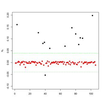
Figure 1: Parameter vector $\theta_{0}$ for the communities dataset. The entries with magnitude larger than $0.04$ (shown in black) are treated as significant ones.

We do the following preprocessing steps: $(i)$ Each missing value is replaced by the mean of the non-missing values of that attribute for other communities; $(ii)$ We eliminate $16$ attributes to make the ensemble of the attribute vectors linearly independent; $(iii)$ We normalize the columns to have mean zero and $\ell_{2}$ norm $\sqrt{n}$. Thus we obtain a design matrix ${\mathbf{X}}_{{\rm tot}}\in{\mathbb{R}}^{n_{{\rm tot}}\times p}$ with $n_{{\rm tot}}=1994$ and $p=106$.

For the sake of performance evaluation, we need to know the true model, i.e., the true significant covariates. We let $\theta_{0}=({\mathbf{X}}_{{\rm tot}}^{\sf T}{\mathbf{X}}_{{\rm tot}})^{-1}{\mathbf{X}}_{{\rm tot}}^{\sf T}y$ be the least square solution obtained from the whole dataset ${\mathbf{X}}_{{\rm tot}}$. The entries of $\theta_{0}$ are shown in Fig. 1. Clearly only a few of them are non negligible, corresponding to the true model. We treat the entries with magnitude larger than $0.04$ as truly active and the others as truly inactive. The number of active covariates according to this criterion is $s_{0}=13$.

We choose random subsamples of size $n=85$ from the communities and normalize each column of the resulting design matrix to have mean zero and $\ell_{2}$ norm $\sqrt{n}$. We use Gauss-Lasso selector and Lasso for model selection based on this design. Figures 2 and 3 respectively show the solution path for Gauss-Lasso and Lasso as the parameter $\lambda$ changes form $\lambda=0.001$ to $\lambda=1$. The paths corresponding to the truly active set are in black and the paths corresponding to the truly inactive variables are in red. At $\lambda=1$, the solutions $\widehat{\theta}^{{\rm GL}}(\lambda)$ and $\widehat{\theta}^{n}(\lambda)$ have no active variables; for decreasing $\lambda$, each knot $\lambda_{k}$ marks the entry or removal of some variables from the current active set of the Lasso solution. Therefore, the support of the Lasso solution $T$ remains constant in between knots. Since Gauss-Lasso selector performs ordinary least squares restricted to $T$, its coordinate paths are constant in between knots. However, the Lasso paths are linear with respect to $\lambda$, with changes in slope at the knots (see e.g., [EHJT04] for a discussion).

It is clear from Figure 3 that the Lasso support either misses a large fraction of the truly active covariates, or includes many false positives. For instance at $\lambda=0.08$, we get $4$ true positives out of $13$ and $4$ false positives. On the other hand, for a smaller value of the regularization parameter, $\lambda=0.01$, we get $10$ true positives out of $13$ and $8$ false positives.

If we consider on the other hand the Gauss-Lasso, any $\lambda\leq 0.02$ produces a set of coefficients with a gap between large ones, that are mostly true positives, and small ones, that are mostly true negatives.

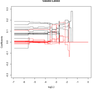
Figure 2: Coordinate paths for Gauss-Lasso selector and a random subset of $n=85$ communities. The paths corresponding to the significant variables of $\theta_{0}$ are shown in black. The coordinate paths for Gauss-Lasso are piecewise constant.

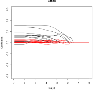
Figure 3: Coordinate paths for Lasso selector and a random subset of $n=85$ communities. The paths corresponding to the significant variables of $\theta_{0}$ are shown in black. The coordinate paths for Lasso are piecewise linear.

5 Proof of Theorems 2.5 and 2.7

In this section we prove Theorems 2.5 and 2.7 using Lemmas 2.1 to 2.4. The latter are proved in the appendices.

5.1 Proof of Theorem 2.5

By the condition 1 in the statement of the theorem, we have

$$\lambda<\min_{i\in S}\left|\frac{\theta_{0,i}}{[\widehat{\Sigma}_{T_{0},T_{0}}^{-1}v_{0,T_{0}}]_{i}}\right|=\xi_{0}\,,$$

where the equality holds because of Lemma 2.2. By Lemma 2.2, we know that ${\rm sign}(\widehat{\theta}^{{\rm ZN}}(\lambda))=v_{0}$ and that ${\rm supp}(v_{0})=T_{0}$ contains the true support $S$. Applying Lemma 2.3, Eq. (9) and using the generalized irrepresentability assumption (10), we obtain

$$\Big{\|}\widehat{\Sigma}_{{T_{0}}^{c},T_{0}}\widehat{\Sigma}_{T_{0},T_{0}}^{-1}v_{0,T_{0}}\Big{\|}_{\infty}\leq 1-\eta\,,$$ (26)

$$v_{0,T_{0}}={\rm sign}\Big{(}\theta_{0,T_{0}}-\lambda\widehat{\Sigma}_{T_{0},T_{0}}^{-1}v_{0,T_{0}}\Big{)}\,.$$ (27)

Also, by Lemma 2.4, ${\rm sign}(\widehat{\theta}^{n})=v_{0}$ if Eqs. (11) and (12) hold with $z=v_{0}$ and $T=T_{0}$, namely, if

$$\Big{\|}\widehat{\Sigma}_{{T_{0}}^{c},T_{0}} \widehat{\Sigma}_{T_{0},T_{0}}^{-1}v_{0,T_{0}}+\frac{1}{\lambda}(\widehat{r}_{{T_{0}}^{c}}-\widehat{\Sigma}_{{T_{0}}^{c},T_{0}}\widehat{\Sigma}_{T_{0},T_{0}}^{-1}\widehat{r}_{T_{0}})\Big{\|}_{\infty}\leq 1\,,$$ (28)

$$v_{0,T_{0}}={\rm sign}\Big{(}\theta_{0,T}-\widehat{\Sigma}^{-1}_{T_{0},T_{0}}(\lambda v_{0,T_{0}}-\widehat{r}_{T_{0}})\Big{)}\,.$$ (29)

In the sequel, we show that these equations are satisfied, with probability lower bounded as per Eq. (16).

We begin with proving Eq. (28). Let $\mathcal{T}=(1/\lambda)(\widehat{r}_{{T_{0}}^{c}}-\widehat{\Sigma}_{{T_{0}}^{c},T_{0}}\widehat{\Sigma}_{T_{0},T_{0}}^{-1}\widehat{r}_{T_{0}})$. We need to show that $\|\mathcal{T}\|_{\infty}\leq\eta$. Plugging for $\widehat{r}$, we get $\mathcal{T}\equiv{\mathbf{X}}_{T_{0}^{c}}\Pi_{{\mathbf{X}}^{\perp}_{T_{0}}}W/(n\lambda)$, where $\Pi_{{\mathbf{X}}^{\perp}_{T_{0}}}={\rm I}-{\mathbf{X}}_{T_{0}}({\mathbf{X}}_{T_{0}}^{\sf T}{\mathbf{X}}_{T_{0}})^{-1}{\mathbf{X}}_{T_{0}}^{\sf T}$ is the orthogonal projection onto the orthogonal complement of the column space of ${\mathbf{X}}_{T_{0}}$. Since $W\sim{\sf N}(0,\sigma^{2}{\rm I}_{n\times n})$, the variable $\mathcal{T}_{j}=x_{j}^{\sf T}\Pi_{{\mathbf{X}}^{\perp}_{T_{0}}}W/(n\lambda)$ is normal with variance at most

$$\Big{(}\frac{\sigma}{n\lambda}\Big{)}^{2}\|\Pi_{{\mathbf{X}}^{\perp}_{T_{0}}}x_{j}\|_{2}^{2}\leq\Big{(}\frac{\sigma}{n\lambda}\Big{)}^{2}\|x_{j}\|_{2}^{2}\leq\frac{\sigma^{2}}{n\lambda^{2}}\,,$$

where we used the fact that $\|x_{j}\|^{2}\leq n$, as $\widehat{\Sigma}_{i,i}\leq 1$. By the Gaussian tail bound with union bound over $j\in T_{0}^{c}$, we obtain

$${\mathbb{P}}(\|\mathcal{T}\|_{\infty}\leq\eta)\geq 1-2pe^{-\frac{n\lambda^{2}\eta^{2}}{2\sigma^{2}}}=1-2p^{1-c_{1}}\,.$$ (30)

We next prove Eq. (29). Given Eq. (27), we need to show

$${\rm sign}\Big{(}\theta_{0,T_{0}}-\lambda\widehat{\Sigma}^{-1}_{T_{0},T_{0}}v_{0,T_{0}}\Big{)}={\rm sign}\Big{(}\theta_{0,T_{0}}-\widehat{\Sigma}^{-1}_{T_{0},T_{0}}(\lambda v_{0,T_{0}}-\widehat{r}_{T_{0}})\Big{)}\,.$$

Let $u\equiv\theta_{0,T_{0}}-\lambda\widehat{\Sigma}^{-1}_{T_{0},T_{0}}v_{0,T_{0}}$, and $\widehat{u}\equiv\theta_{0,T_{0}}-\widehat{\Sigma}^{-1}_{T_{0},T_{0}}(\lambda v_{0,T_{0}}-\widehat{r}_{T_{0}})$.

By condition 1, we have, for all $i\in S$, $|u_{i}|\geq|\theta_{0,i}|-\lambda|[\widehat{\Sigma}^{-1}_{T_{0},T_{0}}v_{0,T_{0}}]_{i}|\geq c_{2}\lambda$. Further, for all $i\in T_{0}\setminus S$, we have $|u_{i}|=\lambda|[\widehat{\Sigma}^{-1}_{T_{0},T_{0}}v_{0,T_{0}}]_{i}|\geq c_{2}\lambda$. Summarizing, for all $i\in T_{0}$, we have $|u_{i}|\geq c_{2}\lambda$. We will show that $\|u-\widehat{u}\|_{\infty}=\|\widehat{\Sigma}^{-1}_{T_{0},T_{0}}\widehat{r}_{T_{0}}\|_{\infty}<c_{2}\lambda$, with high probability, thus implying ${\rm sign}(u_{T_{0}})={\rm sign}(\widehat{u}_{T_{0}})$ as desired.

Lemma 5.1.

The following holds true.

$${\mathbb{P}}\Big{(}\|\widehat{\Sigma}_{T_{0},T_{0}}^{-1}\widehat{r}_{T_{0}}\|_{\infty}\geq\sigma\sqrt{\frac{2c_{1}\log p}{n}}\,\|\widehat{\Sigma}^{-1}_{T_{0},T_{0}}\|_{2}^{1/2}\Big{)}\leq 2p^{1-c_{1}}\,.$$ (31)

Lemma 5.1 is proved by noting that conditioned on ${\mathbf{X}}_{T_{0}}$, $\widehat{\Sigma}_{T_{0},T_{0}}^{-1}\widehat{r}_{T_{0}}$ is a Gaussian vector and then applying standard tail bound inequality. The details are deferred to Section A.5.

Using Lemma 5.1 and the assumption $\eta\leq c_{2}\sqrt{C_{\min}}$, we get $\|u-\widehat{u}\|_{\infty}<c_{2}\lambda$, with probability at least $1-2p^{1-c_{1}}$.

Putting all this together, Eqs. (28) and (29) hold simultaneously, with probability at least $1-4p^{1-c_{1}}$. This implies the thesis.

5.2 Proof of Theorem 2.7

Recall that $T={\rm supp}(\widehat{\theta}^{n})$. On the event $\mathcal{E}\equiv\{T=T_{0}\}$, we have

$$\widehat{\theta}^{{\rm GL}}_{T}=({\mathbf{X}}_{T}^{\sf T}{\mathbf{X}}_{T})^{-1}{\mathbf{X}}_{T}^{\sf T}({\mathbf{X}}_{T}\theta_{0,T}+W)=\theta_{0,T}+({\mathbf{X}}_{T}^{\sf T}{\mathbf{X}}_{T})^{-1}{\mathbf{X}}_{T}^{\sf T}W\,,$$

where the first equality holds since $T=T_{0}\supseteq S$ and thus $\theta_{0,T^{c}}=0$. Further note that $\widehat{\theta}^{{\rm GL}}_{i}-\theta_{0,i}$, for $i\in T$, is a zero mean Gaussian vector with variance

$$\sigma^{2}\|e_{i}^{\sf T}({\mathbf{X}}_{T}^{\sf T}{\mathbf{X}}_{T})^{-1}{\mathbf{X}}_{T}^{\sf T}\|^{2}\leq\sigma^{2}\|\widehat{\Sigma}^{-1}_{T,T}\|_{2}/n\leq\sigma^{2}/(nC_{\min})\,.$$

Using tail bound inequality along with union bounding over $i\in[p]$, we get

$${\mathbb{P}}\Big{(}\|\widehat{\theta}^{{\rm GL}}_{T}-\theta_{0,T}\|_{\infty}\geq\mu;\mathcal{E}\Big{)}\leq 2e^{-nC_{\min}\mu^{2}/2\sigma^{2}}\,.$$

Also, under the assumptions of Theorem 2.5, ${\mathbb{P}}(\mathcal{E})\geq 1-4p^{1-c_{1}}$. Hence

$${\mathbb{P}}\Big{(}\|\widehat{\theta}^{{\rm GL}}_{T}-\theta_{0,T}\|_{\infty}\geq\mu\Big{)}\leq{\mathbb{P}}\Big{(}\|\widehat{\theta}^{{\rm GL}}_{T}-\theta_{0,T}\|_{\infty}\geq\mu;\mathcal{E}\Big{)}+{\mathbb{P}}(\mathcal{E}^{c})\leq 2e^{-nC_{\min}\mu^{2}/2\sigma^{2}}+4p^{1-c_{1}}\,.$$

Since $\widehat{\theta}^{{\rm GL}}_{T^{c}}=\theta_{0,T^{c}}=0$, we get $\|\widehat{\theta}^{{\rm GL}}-\theta_{0}\|_{\infty}<\mu$, with probability at least $1-4p^{1-c_{1}}-2e^{-nC_{\min}\mu^{2}/2\sigma^{2}}$.

Moreover, if $\|\widehat{\theta}^{{\rm GL}}-\theta_{0}\|<\theta_{\min}/2$, then $|\widehat{\theta}^{{\rm GL}}_{i}|>\theta_{\min}/2$ for $i\in S$ and $|\widehat{\theta}^{{\rm GL}}_{i}|<\theta_{\min}/2$, for $i\in S^{c}$. Hence, the $s_{0}$ top entries of $\widehat{\theta}^{{\rm GL}}$ (in modulus), returned by the Gauss-Lasso selector, correspond to the true support $S$. Therefore,

$${\mathbb{P}}(\hat{S}=S) \geq{\mathbb{P}}(\|\widehat{\theta}^{{\rm GL}}-\theta_{0}\|_{\infty}<\theta_{\min}/2)$$

$$\geq 1-4p^{1-c_{1}}-2pe^{-nC_{\min}\theta_{\min}^{2}/8\sigma^{2}}\geq 1-6p^{1-c_{1}/4}\,,$$

where the last inequality follows from the facts $\theta_{\min}\geq c_{2}\lambda$, and $\eta\leq c_{2}\sqrt{C_{\min}}$.

6 Proof of Theorems 3.4 and 3.7

By the condition 1 in the statement of the theorem, we have

$$\lambda\leq\frac{2}{3}\min_{i\in S}\left|\frac{\theta_{0,i}}{[\Sigma_{T_{0},T_{0}}^{-1}v_{0,T_{0}}]_{i}}\right|<\xi_{0}\,,$$

where the second inequality holds because of Lemma 3.2. Therefore, as a result of Lemma 3.2, we have ${\rm sign}(\widehat{\theta}^{\infty}(\lambda))=v_{0}$ and that ${\rm supp}(v_{0})=T_{0}$ contains the true support $S$. Applying Lemma 3.3 and using the generalized irrepresentability assumption, we have

$$\Big{\|}\Sigma_{{T_{0}}^{c},T_{0}}\Sigma_{T_{0},T_{0}}^{-1}v_{0,T_{0}}\Big{\|}_{\infty}\leq 1-\eta\,,$$ (32)

$$v_{0,T_{0}}={\rm sign}\Big{(}\theta_{0,T_{0}}-\lambda\Sigma_{T_{0},T_{0}}^{-1}v_{0,T_{0}}\Big{)}\,.$$ (33)

Moreover, by Lemma 2.4, ${\rm sign}(\widehat{\theta}^{n})=v_{0}$ if Eqs. (11) and (12) hold with $z=v_{0}$ and $T=T_{0}$, namely,

$$\Big{\|}\widehat{\Sigma}_{{T_{0}}^{c},T_{0}} \widehat{\Sigma}_{T_{0},T_{0}}^{-1}v_{0,T_{0}}+\frac{1}{\lambda}(\widehat{r}_{{T_{0}}^{c}}-\widehat{\Sigma}_{{T_{0}}^{c},T_{0}}\widehat{\Sigma}_{T_{0},T_{0}}^{-1}\widehat{r}_{T_{0}})\Big{\|}_{\infty}\leq 1\,,$$ (34)

$$v_{0,T_{0}}={\rm sign}\Big{(}\theta_{0,T}-\widehat{\Sigma}^{-1}_{T_{0},T_{0}}(\lambda v_{0,T_{0}}-\widehat{r}_{T_{0}})\Big{)}\,.$$ (35)

The rest of the proof is devoted to show the validity of these equations, with probability lower bounded as per Eq. (24).

6.1 Proof of Eq. (34)

It is immediate to see that Eq. (34) holds if the followings hold true:

$$\mathcal{T}_{1}\equiv\big{\|}\widehat{\Sigma}_{{T_{0}}^{c},T_{0}}\widehat{\Sigma}^{-1}_{T_{0},T_{0}}v_{0,T_{0}}\big{\|}_{\infty}\leq 1-\frac{\eta}{2}\,,$$ (36)

$$\mathcal{T}_{2}\equiv\frac{1}{\lambda}\big{\|}\widehat{r}_{{T_{0}}^{c}}-\widehat{\Sigma}_{{T_{0}}^{c},T_{0}}\widehat{\Sigma}^{-1}_{T_{0},T_{0}}\widehat{r}_{T_{0}}\big{\|}_{\infty}\leq\frac{\eta}{2}\,.$$ (37)

In order to prove inequalities (36) and (37), it is useful to recall the following proposition from random matrix theory.

Proposition 6.1 ([DS01, Wai09, Ver12]).

For $k\leq n$, let ${\mathbf{X}}\in{\mathbb{R}}^{n\times k}$ be a random matrix with i.i.d rows drawn from ${\sf N}(0,\Sigma)$. Then the following hold true for all $t\geq 1$ and $\tau\equiv 2(\sqrt{\frac{k}{n}}+t)+(\sqrt{\frac{k}{n}}+t)^{2}$ .

• If $\Sigma$ has maximum eigenvalue $\sigma_{\max}<\infty$, then

  $${\mathbb{P}}\bigg{(}\|\frac{1}{n}{\mathbf{X}}^{\sf T}{\mathbf{X}}-\Sigma\|_{2}\geq\sigma_{\max}\,\tau\bigg{)}\leq 2e^{-nt^{2}/2}\,.$$

• If $\Sigma$ has minimum eigenvalue $\sigma_{\min}>0$, then

  $${\mathbb{P}}\bigg{(}\|(\frac{1}{n}{\mathbf{X}}^{\sf T}{\mathbf{X}})^{-1}-\Sigma^{-1}\|_{2}\geq\sigma_{\min}^{-1}\,\tau\bigg{)}\leq 2e^{-nt^{2}/2}\,.$$

We consider the particular choice of $t=\sqrt{k/n}$ which is useful for future reference. Since $k/n\leq 1$, we get $\tau\leq 8\sqrt{k/n}$ and therefore the specialized version of Proposition 6.1 reads:

$${\mathbb{P}}\bigg{(}\|\frac{1}{n}{\mathbf{X}}^{\sf T}{\mathbf{X}}-\Sigma\|_{2}\geq 8\sqrt{k/n}\,\sigma_{\max}\bigg{)} \leq 2e^{-k/2}\,,$$ (38)

$${\mathbb{P}}\bigg{(}\|(\frac{1}{n}{\mathbf{X}}^{\sf T}{\mathbf{X}})^{-1}-\Sigma^{-1}\|_{2}\geq 8\sqrt{k/n}\,\sigma_{\min}^{-1}\bigg{)} \leq 2e^{-k/2}\,.$$ (39)

We define the event $\mathcal{E}_{1}$ as

$$\mathcal{E}_{1} \equiv\bigg{\{}\|(\widehat{\Sigma}_{T_{0},T_{0}})^{-1}-\Sigma_{T_{0},T_{0}}^{-1}\|_{2}\leq 8\sqrt{t_{0}/n}\,C_{\min}^{-1}\bigg{\}}\,.$$

Applying Eqs. (38), (39) to ${\mathbf{X}}_{T_{0}}$, we conclude that

$${\mathbb{P}}(\mathcal{E}_{1}^{c})\leq 2e^{-t_{0}/2}\,.$$ (40)

We now have in place all we need to bound the terms $\mathcal{T}_{1}$ and $\mathcal{T}_{2}$.

6.1.1 Bounding $\mathcal{T}_{1}$

To bound $\mathcal{T}_{1}$, we employ similar techniques to those used in [Wai09, Theorem 3] to verify strict dual feasibility. The argument in [Wai09] works under the irrepresentability condition (see Eq. (26) therein) and we modify it to apply to the current setting, i.e., the generalized irrepresentability condition.

We begin by conditioning on ${\mathbf{X}}_{T_{0}}$. For $j\in{T_{0}}^{c}$, $x_{j}$ is a zero mean Gaussian vector and we can decompose it into a linear correlated part plus an uncorrelated part as

$$x_{j}^{\sf T}=\Sigma_{j,T_{0}}\Sigma_{T_{0},T_{0}}^{-1}{\mathbf{X}}_{T_{0}}^{\sf T}+\epsilon_{j}^{\sf T}\,,$$

where $\epsilon_{j}\in{\mathbb{R}}^{n}$ has i.i.d. entries distributed as $\epsilon_{ji}\sim{\sf N}(0,\Sigma_{j,j}-\Sigma_{j,T_{0}}\Sigma_{T_{0},T_{0}}^{-1}\Sigma_{T_{0},j})$.

Letting $u=\widehat{\Sigma}_{{T_{0}}^{c},T_{0}}\widehat{\Sigma}^{-1}_{T_{0},T_{0}}v_{0,T_{0}}$, we write

$$u_{j} =x_{j}^{\sf T}{\mathbf{X}}_{T_{0}}({\mathbf{X}}_{T_{0}}^{\sf T}{\mathbf{X}}_{T_{0}})^{-1}v_{0,T_{0}}$$

$$=\Sigma_{j,T_{0}}(\Sigma_{T_{0},T_{0}})^{-1}v_{0,T_{0}}+\epsilon_{j}^{\sf T}{\mathbf{X}}_{T_{0}}({\mathbf{X}}_{T_{0}}^{\sf T}{\mathbf{X}}_{T_{0}})^{-1}v_{0,T_{0}}\,.$$ (41)

The first term is bounded as $|\Sigma_{j,T_{0}}(\Sigma_{T_{0},T_{0}})^{-1}v_{0,T_{0}}|\leq 1-\eta$ as per Eq. (32). Let $m_{j}=\epsilon_{j}^{\sf T}{\mathbf{X}}_{T_{0}}({\mathbf{X}}_{T_{0}}^{\sf T}{\mathbf{X}}_{T_{0}})^{-1}v_{0,T_{0}}$. Since ${\rm Var}(\epsilon_{ji})\leq\Sigma_{j,j}\leq 1$, conditioned on ${\mathbf{X}}_{T_{0}}$, $m_{j}$ is zero mean Gaussian with variance at most

$${\rm Var}(m_{j}) \leq\|{\mathbf{X}}_{T_{0}}({\mathbf{X}}_{T_{0}}^{\sf T}{\mathbf{X}}_{T_{0}})^{-1}v_{0,T_{0}}\|_{2}^{2}$$

$$\leq\frac{1}{n}v_{0,T_{0}}^{\sf T}\Big{(}\frac{{\mathbf{X}}_{T_{0}}^{\sf T}{\mathbf{X}}_{T_{0}}}{n}\Big{)}^{-1}v_{0,T_{0}}$$

$$\leq\frac{1}{n}\|\widehat{\Sigma}_{T_{0},T_{0}}^{-1}\|_{2}\,\|v_{0,T_{0}}\|^{2}\,.$$ (42)

Under the event $\mathcal{E}_{1}$, we have

$$\|\widehat{\Sigma}^{-1}_{T_{0},T_{0}}\|_{2}\leq\|\Sigma_{T_{0},T_{0}}^{-1}\|_{2}+\|\widehat{\Sigma}_{T_{0},T_{0}}^{-1}-\Sigma_{T_{0},T_{0}}^{-1}\|_{2}\leq(1+8\sqrt{t_{0}/n})\,C_{\min}^{-1}\leq 9C_{\min}^{-1}\,,$$ (43)

and hence, ${\rm Var}(m_{j})\leq 9t_{0}/(nC_{\min})$. We now define the event $\mathcal{E}$ as

$$\mathcal{E}\equiv\bigg{\{}\max_{j\in T^{c}}|m_{j}|\geq\sqrt{\frac{18c_{1}\,t_{0}\log p}{n\,C_{\min}}}\bigg{\}}\,.$$

By the total probability rule, we have

$${\mathbb{P}}(\mathcal{E})\leq{\mathbb{P}}(\mathcal{E};\mathcal{E}_{1})+{\mathbb{P}}(\mathcal{E}_{1}^{c})\,.$$

Using Gaussian tail bound and union bounding over $j\in{T_{0}}^{c}$, we obtain ${\mathbb{P}}(\mathcal{E};\mathcal{E}_{1})\leq 2p^{1-c_{1}}$. Using the bound ${\mathbb{P}}(\mathcal{E}_{1}^{c})\leq 2e^{-t_{0}/2}$, we arrive at:

$${\mathbb{P}}\left(\max_{j\in T^{c}}|m_{j}|>\sqrt{\frac{18c_{1}\,t_{0}\log p}{n\,C_{\min}}}\right)\leq 2p^{1-c_{1}}+2e^{-\frac{t_{0}}{2}}\,.$$ (44)

Using this, together with Eq. (32), in Eq. (41), we obtain that the following holds true with probability at least $1-2p^{1-c_{1}}-2e^{-t_{0}/2}$:

$$\mathcal{T}_{1}\leq 1-\eta+\sqrt{\frac{18c_{1}\,t_{0}\log p}{n\,C_{\min}}}\,.$$ (45)

It is easy to check that the this implies $\mathcal{T}_{1}<1-\eta/2$, for $\lambda$ as claimed in Eq. (21) provided $n\geq M_{1}t_{0}\log p$.

6.1.2 Bounding $\mathcal{T}_{2}$

We bound $\mathcal{T}_{2}$ by the same technique used in proving Eq. (28). Let $m=(1/\lambda)(\widehat{r}_{{T_{0}}^{c}}-\widehat{\Sigma}_{{T_{0}}^{c},T_{0}}\widehat{\Sigma}_{T_{0},T_{0}}^{-1}\widehat{r}_{T_{0}})$. Plugging for $\widehat{r}$, we get $m\equiv{\mathbf{X}}_{T_{0}^{c}}\Pi_{{\mathbf{X}}^{\perp}_{T_{0}}}W/(n\lambda)$. Since $W\sim{\sf N}(0,\sigma^{2}{\rm I}_{n\times n})$, conditioned on ${\mathbf{X}}$, the variable $m_{j}=x_{j}^{\sf T}\Pi_{{\mathbf{X}}^{\perp}_{T_{0}}}W/(n\lambda)$ is normal with variance at most

$$(\frac{\sigma}{n\lambda})^{2}\|\Pi_{{\mathbf{X}}^{\perp}_{T_{0}}}x_{j}\|_{2}^{2}\leq(\frac{\sigma}{n\lambda})^{2}\|x_{j}\|^{2}\,,$$

where we used the contraction property of orthogonal projections. Now, define the event $\mathcal{E}$ as follows.

$$\mathcal{E}\equiv\bigg{\{}\|x_{j}\|^{2}<2n,\forall j\in[p]\bigg{\}}\,.$$

Note that $\|x_{j}\|^{2}\stackrel{{\scriptstyle\text{\rm d}}}{{=}}\Sigma_{j,j}Z$, where $Z$ is a chi-squared random variable with $n$ degrees of freedom. Using the standard chi-squared tail bounds [Joh01], for a fixed $j$, we have $\|x_{j}\|^{2}<2\Sigma_{j,j}\,n\leq 2n$, with probability at least $1-e^{-n/10}$. Union bounding over $j\in[p]$, we obtain ${\mathbb{P}}(\mathcal{E}^{c})\leq pe^{-n/10}$.

Under the event $\mathcal{E}$, we have ${\rm Var}(m_{j})\leq 2\sigma^{2}/(n\lambda^{2})$. Employing the standard Gaussian tail bound along with union bounding over $j\in T_{0}^{c}$, we obtain

$${\mathbb{P}}(\mathcal{T}_{2}\geq\eta/2;\,\mathcal{E})\leq 2pe^{-\frac{n\lambda^{2}\eta^{2}}{16\sigma^{2}}}=2p^{1-c_{1}}\,.$$ (46)

Hence,

$${\mathbb{P}}(\mathcal{T}_{2}\geq\eta/2)\leq{\mathbb{P}}(\mathcal{T}_{2}\geq\eta/2;\,\mathcal{E})+{\mathbb{P}}(\mathcal{E}^{c})\leq 2p^{1-c_{1}}+pe^{-\frac{n}{10}}\,.$$ (47)

6.2 Proof of Eq. (35)

We next prove Eq. (35). Given Eq. (33), we need to show

$${\rm sign}\Big{(}\theta_{0,T_{0}}-\lambda\Sigma^{-1}_{T_{0},T_{0}}v_{0,T_{0}}\Big{)}={\rm sign}\Big{(}\theta_{0,T_{0}}-\widehat{\Sigma}^{-1}_{T_{0},T_{0}}(\lambda v_{0,T_{0}}-\widehat{r}_{T_{0}})\Big{)}\,.$$

Let $u\equiv\theta_{0,T_{0}}-\lambda\Sigma^{-1}_{T_{0},T_{0}}v_{0,T_{0}}$, and $\widehat{u}\equiv\theta_{0,T_{0}}-\widehat{\Sigma}^{-1}_{T_{0},T_{0}}(\lambda v_{0,T_{0}}-\widehat{r}_{T_{0}})$.

By condition 1, we have, for all $i\in S$, $|u_{i}|\geq|\theta_{0,i}|-\lambda|[\Sigma^{-1}_{T_{0},T_{0}}v_{0,T_{0}}]_{i}|\geq c_{2}\lambda+(1/2)\lambda|[\Sigma^{-1}_{T_{0},T_{0}}v_{0,T_{0}}]_{i}|$. Further, for all $i\in T_{0}\setminus S$, we have $|u_{i}|=\lambda|[\Sigma^{-1}_{T_{0},T_{0}}v_{0,T_{0}}]_{i}|\geq c_{2}\lambda+(1/2)\lambda|[\Sigma^{-1}_{T_{0},T_{0}}v_{0,T_{0}}]_{i}|$. Summarizing, for all $i\in T_{0}$, we have

$$|u_{i}|\geq c_{2}\lambda+\frac{1}{2}\lambda|[\Sigma^{-1}_{T_{0},T_{0}}v_{0,T_{0}}]_{i}|\,.$$

We will show that $|u_{i}-\widehat{u}_{i}|<c_{2}\lambda+(1/2)\lambda|[\Sigma^{-1}_{T_{0},T_{0}}v_{0,T_{0}}]_{i}|$ for all $i\in T_{0}$, with high probability, thus implying ${\rm sign}(u_{T_{0}})={\rm sign}(\widehat{u}_{T_{0}})$ as desired. Since $|u_{i}-\widehat{u}_{i}|\leq\lambda|[(\widehat{\Sigma}_{T_{0},T_{0}}^{-1}-\Sigma_{T_{0},T_{0}}^{-1})v_{0,T_{0}}]_{i}|+|[\widehat{\Sigma}^{-1}_{T_{0},T_{0}}\widehat{r}_{T_{0}}]_{i}|$, it suffices to show that

$$\mathcal{T}_{3}(i)\equiv\lambda|[(\widehat{\Sigma}_{T_{0},T_{0}}^{-1}-\Sigma_{T_{0},T_{0}}^{-1})v_{0,T_{0}}]_{i}\big{|}<\frac{1}{2}\lambda|[\Sigma^{-1}_{T_{0},T_{0}}v_{0,T_{0}}]_{i}|\,\;\;\;\;\;\;\mbox{for all }i\in T_{0},$$ (48)

$$\mathcal{T}_{4}\equiv\|\widehat{\Sigma}_{T_{0},T_{0}}^{-1}\widehat{r}_{T_{0}}\|_{\infty}<c_{2}\lambda\,.$$ (49)

In the sequel, we provide probabilistic bounds on $\mathcal{T}_{3}(i)$ and $\mathcal{T}_{4}$.

6.2.1 Bounding $\mathcal{T}_{3}(i)$

Lemma 6.2.

Under the assumptions of Theorem 3.4, for any $c^{\prime}>1$, $t_{0}\geq 4$, we have

$${\mathbb{P}}\left\{\exists i\in T_{0}\;\;\mbox{{\rm s.t. }}\big{|}[(\widehat{\Sigma}_{T_{0},T_{0}}^{-1}-\Sigma_{T_{0},T_{0}}^{-1})v_{0,T_{0}}]_{i}\big{|}\geq 16\sqrt{\frac{c^{\prime}c_{*}\,t_{0}\log p}{n}}\big{|}[\Sigma_{T_{0},T_{0}}^{-1}v_{0,T_{0}}]_{i}\big{|}\right\}\leq 2e^{-\frac{t_{0}}{2}}+2p^{1-c^{\prime}}\,,$$

where $c_{*}\equiv(c_{2}C_{\min})^{-2}$.

The proof of Lemma 6.2 is presented in Section A.6.

Applying this lemma, with probability at least $1-2e^{-t_{0}/2}-2p^{1-c_{1}}$, we have $\mathcal{T}_{3}(i)<(1/2)\lambda|[\Sigma^{-1}_{T_{0},T_{0}}v_{0,T_{0}}]_{i}|$ provided

$$16\sqrt{\frac{c_{1}c_{*}\,t_{0}\log p}{n}}\leq\frac{1}{2}\,.$$

i.e., for $n\geq M_{3}t_{0}\log p$.

6.2.2 Bounding $\mathcal{T}_{4}$

Lemma 6.3.

The following holds true.

$${\mathbb{P}}\bigg{(}\mathcal{T}_{4}\leq 3\sigma\sqrt{\frac{2c_{1}\log p}{n\,C_{\min}}}\bigg{)}\geq 1-2e^{-\frac{t_{0}}{2}}-2p^{1-c_{1}}\,.$$ (50)

Lemma 6.3 is proved in Section A.7.

From the last lemma, it follows that Eq. (49) holds with probability at least $1-2e^{-\frac{t_{0}}{2}}-2p^{1-c_{1}}$, provided

$$3\sigma\sqrt{\frac{2c_{1}\log p}{n\,C_{\min}}}\leq c_{2}\lambda\,.$$

Choosing $\lambda$ as per Eq. (21), the latter is easily shown to follow from $\eta\leq c_{2}\sqrt{C_{\min}}$.

6.3 Summary: Proof of Theorem 3.4

Now combining the bounds on $\mathcal{T}_{1}$,…$\mathcal{T}_{4}$, we get that for $n\geq\max(M_{1},M_{3})\,t_{0}\log p$, Eqs. (34) and (35) hold simultaneously, with probability at least $1-pe^{-n/10}-6e^{-t_{0}/2}-8p^{1-c_{1}}$. This implies ${\rm sign}(\widehat{\theta}^{n}(\lambda))=v_{0}$.

6.4 Proof of Theorem 3.7

Note that the matrix ${\mathbf{X}}_{T_{0}}$ is a random Gaussian matrix with rows drawn independently form ${\sf N}(0,\Sigma_{T_{0},T_{0}})$ (recall that $T_{0}$ is a deterministic set determined by the population-level problem). Therefore, $\|\widehat{\Sigma}_{T_{0},T_{0}}^{-1}\|_{2}\leq 9\|\Sigma_{T_{0},T_{0}}^{-1}\|_{2}\leq 9C_{\min}^{-1}$. Using Theorem 3.4 to bound the probability that $T\neq T_{0}$, the proof proceeds along the same lines as the proof of Theorem 2.7.

Appendix A Proof of technical lemmas

A.1 Proof of Lemma 2.1

By a change of variables, it is easy to see that $\widehat{\theta}^{{\rm ZN}}(\xi)=\theta_{0}+\xi\,\widehat{u}(\xi)$, where $\widehat{u}(\xi)=\arg\min_{u\in{\mathbb{R}}^{p}}F(u;\xi)$ and

$$F(u;\xi)\equiv\frac{1}{2}\langle u,\widehat{\Sigma}u\rangle+\|u_{S^{c}}\|_{1}+\Big{(}\|\xi^{-1}\theta_{0,S}+u_{S}\|_{1}-\|\xi^{-1}\theta_{0,S}\|_{1}\Big{)}\,.$$

The rest of the proof is analogous to an argument in [BRT09]. Since, by definition, $F(\widehat{u};\xi)\leq F(0;\xi)$, we have

$$\frac{1}{2}\langle\widehat{u},\widehat{\Sigma}\widehat{u}\rangle+\|\widehat{u}_{S^{c}}\|_{1}-\|\widehat{u}_{S}\|_{1}\leq 0$$ (51)

and hence $\|\widehat{u}_{S^{c}}\|_{1}\leq\|\widehat{u}_{S}\|_{1}$. Using the definition of $\widehat{\kappa}$, with $J=S$, $c_{0}=1$, we have

$$0 \geq\frac{1}{2}\widehat{\kappa}(s_{0},1)\|\widehat{u}\|_{2}^{2}+\|\widehat{u}_{S^{c}}\|_{1}-\|\widehat{u}_{S}\|_{1}$$

$$\geq\frac{1}{2}\widehat{\kappa}(s_{0},1)\|\widehat{u}_{S}\|_{2}^{2}-\|\widehat{u}_{S}\|_{1}\,,$$

and since $\|\widehat{u}_{S}\|_{2}^{2}\geq\|\widehat{u}_{S}\|_{1}^{2}/s_{0}$, we deduce that

$$\|\widehat{u}_{S}\|_{1}\leq\frac{2s_{0}}{\widehat{\kappa}(s_{0},1)}\,.$$

By Eq. (51), this implies in turn

$$\langle\widehat{u},\widehat{\Sigma}\widehat{u}\rangle\leq\frac{4s_{0}}{\widehat{\kappa}(s_{0},1)}\,.$$ (52)

Now, consider the stationarity conditions of $F$. These imply

$$(\widehat{\Sigma}\widehat{u})_{i} =-{\rm sign}(\widehat{u}_{i})\,,\;\;\;\;\;\;\;\mbox{for $i\in T\setminus S$}.$$

We therefore have

$$|T\setminus S|\leq\sum_{i\in T\setminus S}(\widehat{\Sigma}\widehat{u})_{i}^{2}\leq\|\widehat{\Sigma}\widehat{u}\|_{2}^{2}\leq\|\widehat{\Sigma}\|_{2}\langle\widehat{u},\widehat{\Sigma}\widehat{u}\rangle\,,$$

and our claim follows by substituting Eq. (52) in the latter equation.

A.2 Proof of Lemma 2.2

By a change of variables, it is easy to see that $\widehat{\theta}^{{\rm ZN}}(\xi)=\theta_{0}+\xi\,\widehat{u}(\xi)$, where $\widehat{u}(\xi)=\arg\min_{u\in{\mathbb{R}}^{p}}F(u;\xi)$ and

$$F(u;\xi)\equiv\frac{1}{2}\langle u,\widehat{\Sigma}u\rangle+\|u_{S^{c}}\|_{1}+\Big{(}\|\xi^{-1}\theta_{0,S}+u_{S}\|_{1}-\|\xi^{-1}\theta_{0,S}\|_{1}\Big{)}\,.$$

Notice that, for any $u\in{\mathbb{R}}^{p}$, $\lim_{\xi\to 0}F(u;\xi)=F_{0}(u)$, where

$$F_{0}(u)\equiv\frac{1}{2}\langle u,\widehat{\Sigma}u\rangle+\|u_{S^{c}}\|_{1}+\langle{\rm sign}(\theta_{0,S}),u_{S}\rangle\,.$$

Indeed $F(u;\xi)=F_{0}(u)$ provided $\xi\leq\min_{i\in S}|\theta_{0,i}/u_{i}|$. Further, $F(u;\xi)\geq F_{0}(u)$ for all $u$.

Let $u_{0}\equiv\arg\min_{u\in{\mathbb{R}}^{p}}F_{0}(u)$, and set $\xi_{0}\equiv\min_{i\in S}|\theta_{0,i}/u_{0,i}|$. Then, for any $u\neq u_{0}$, and all $\xi\in(0,\xi_{0})$, we have

$$F(u;\xi)\geq F_{0}(u)>F_{0}(u_{0})=F(u_{0};\xi)\,.$$

Hence $u_{0}$ is the unique minimizer of $F(u;\xi)$, i.e., $\widehat{u}(\xi)=u_{0}$ for all $\xi\in(0,\xi_{0})$.

It follows that $\widehat{\theta}^{{\rm ZN}}(\xi)=\theta_{0}+\xi\,u_{0}$ for all $\xi\in(0,\xi_{0})$ and hence ${\rm sign}(\widehat{\theta}^{{\rm ZN}}(\xi))=v_{0}$ and ${\rm supp}(\widehat{\theta}^{{\rm ZN}}(\xi))=T_{0}$ where we set

$$v_{0,S} \equiv {\rm sign}(\theta_{0,S})\,,$$

$$v_{0,S^{c}} \equiv {\rm sign}(u_{0,S^{c}})\,,$$

$$T_{0} \equiv S\cup{\rm supp}(u_{0})\,.$$

Finally, the zero subgradient condition for $u_{0}$ reads $\widehat{\Sigma}u_{0}+z=0$, with $z_{S}={\rm sign}(\theta_{0,S})$ and $z_{S^{c}}\in\partial\|u_{0,S^{c}}\|_{1}$. In particular, $z_{T_{0}}=v_{0,T_{0}}$ and therefore $u_{0,T_{0}}=-\widehat{\Sigma}_{T_{0},T_{0}}^{-1}v_{T_{0}}$. This implies

$$\xi_{0}\equiv\min_{i\in S}\left|\frac{\theta_{0,i}}{u_{0,i}}\right|=\min_{i\in S}\left|\frac{\theta_{0,i}}{[\widehat{\Sigma}_{T_{0},T_{0}}^{-1}v_{0,T_{0}}]_{i}}\right|\,.$$

A.3 Proof of Lemma 2.3

Writing the zero-subgradient conditions for problem (5), we have

$$\widehat{\Sigma}(\widehat{\theta}^{{\rm ZN}}-\theta_{0})=-\xi u,\quad\quad u\in\partial\|\widehat{\theta}^{{\rm ZN}}\|_{1}.$$

Given that $T\supseteq S$, we have $\theta_{0,T^{c}}=0$, and thus

$$\widehat{\Sigma}_{T,T}(\widehat{\theta}^{{\rm ZN}}_{T}-\theta_{0,T}) =-\xi u_{T}\,,$$

$$\widehat{\Sigma}_{T^{c},T}(\widehat{\theta}^{{\rm ZN}}_{T}-\theta_{0,T}) =-\xi u_{T^{c}}\,.$$

Solving for $\widehat{\theta}^{{\rm ZN}}_{T}-\theta_{0,T}$ in terms of $u_{T}$, we obtain

$$\widehat{\Sigma}_{T^{c},T}\widehat{\Sigma}_{T,T}^{-1}u_{T}=u_{T^{c}}\,,$$

$$\widehat{\theta}^{{\rm ZN}}_{T}=\theta_{0,T}-\xi\widehat{\Sigma}_{T,T}^{-1}u_{T}\,.$$

This proves the ‘only if’ part noting that $u_{T}={\rm sign}(\widehat{\theta}^{{\rm ZN}}_{T})=v_{T}$, and $\|u_{T^{c}}\|_{\infty}\leq 1$ since $u\in\partial\|\widehat{\theta}^{{\rm ZN}}\|_{1}$.

Now suppose that Eqs. (8) and (9) hold true.

Let $\tilde{\theta}_{T}=\theta_{0,T}-\xi\widehat{\Sigma}_{T,T}^{-1}v_{T}$, and $\tilde{\theta}_{T^{c}}=0$. We prove that $\tilde{\theta}=\widehat{\theta}^{{\rm ZN}}$, by showing that it satisfies the zero-subgradient condition. By Eq. (9), $v_{T}={\rm sign}(\tilde{\theta}_{T})$. Define $u\in{\mathbb{R}}^{p}$ by letting $u_{T}=v_{T}$ and $u_{T^{c}}=\widehat{\Sigma}_{T^{c},T}\widehat{\Sigma}_{T,T}^{-1}v_{T}$. Note that $\|u_{T^{c}}\|_{\infty}\leq 1$ by Eq. (8), and so $u\in\partial\|\tilde{\theta}\|_{1}$. Moreover,

$$\widehat{\Sigma}_{T,T}(\tilde{\theta}_{T}-\theta_{0,T}) =-\xi u_{T}\,$$

$$\widehat{\Sigma}_{T^{c},T}(\tilde{\theta}_{T}-\theta_{0,T}) =-\xi u_{T^{c}}\,,$$

Combining the above two equations, we get the zero-subgradient condition for $(\tilde{\theta},u)$. Therefore, $\tilde{\theta}=\widehat{\theta}^{{\rm ZN}}$, and $v={\rm sign}(\widehat{\theta}^{{\rm ZN}})$.

A.4 Proof of Lemma 2.4

The proof proceeds along the same lines as the proof of Lemma 2.3. We begin with proving the ‘only if’ part. The zero-subgradient condition for Problem 3 reads:

$$-\frac{1}{n}{\mathbf{X}}^{\sf T}(Y-{\mathbf{X}}\widehat{\theta}^{n})+\lambda u=0\,,\quad\quad u\in\partial\|\widehat{\theta}^{n}\|_{1}\,.$$

Plugging for $Y={\mathbf{X}}\theta_{0}+W$ and $\widehat{r}=({\mathbf{X}}^{\sf T}W/n)$ in the above equation, we arrive at:

$$\widehat{\Sigma}(\widehat{\theta}^{n}-\theta_{0})=\widehat{r}-\lambda u\,.$$

Since $T\supseteq S$, $\theta_{0,T^{c}}=0$, and writing the above equation for indices in $T$ and $T^{c}$ separately, we obtain

$$\widehat{\Sigma}_{T^{c},T}(\widehat{\theta}^{n}_{T}-\theta_{0,T}) =\widehat{r}_{T^{c}}-\lambda u_{T^{c}}\,,$$

$$\widehat{\Sigma}_{T,T}(\widehat{\theta}^{n}_{T}-\theta_{0,T}) =\widehat{r}_{T}-\lambda u_{T}\,.$$

Solving for $\widehat{\theta}^{n}_{T}-\theta_{0,T}$ from the second equation, we get

$$\widehat{\Sigma}_{T^{c},T}\widehat{\Sigma}_{T,T}^{-1}u_{T} +\frac{1}{\lambda}(\widehat{r}_{T^{c}}-\widehat{\Sigma}_{T^{c},T}\widehat{\Sigma}_{T,T}^{-1}\widehat{r}_{T})=u_{T^{c}}\,,$$

$$\widehat{\theta}^{n}_{T} =\theta_{0,T}-\widehat{\Sigma}_{T,T}^{-1}(\lambda u_{T}-\widehat{r}_{T})\,.$$

This proves Eqs. (11) and (12), since $u_{T}={\rm sign}(\widehat{\theta}^{n}_{T})=z_{T}$ and $\|u_{T^{c}}\|_{\infty}\leq 1$.

We next prove the other direction. Suppose that Eqs. (11) and (12) hold true. Let $\tilde{\theta}_{T}=\theta_{0,T}-\widehat{\Sigma}_{T,T}^{-1}(\lambda z_{T}-\widehat{r}_{T})$, and $\tilde{\theta}_{T^{c}}=0$. We prove that $\tilde{\theta}=\widehat{\theta}^{n}$, by showing that it satisfies the zero-subgradient condition. By Eq. (12), $z_{T}={\rm sign}(\tilde{\theta}_{T})$. Define $u\in{\mathbb{R}}^{p}$ by letting $u_{T}=z_{T}$ and $u_{T^{c}}=\widehat{\Sigma}_{T^{c},T}\widehat{\Sigma}_{T,T}^{-1}z_{T}+(\widehat{r}_{T^{c}}-\widehat{\Sigma}_{T^{c},T}\widehat{\Sigma}^{-1}_{T,T}\widehat{r}_{T})/\lambda$. Note that $\|u_{T^{c}}\|_{\infty}\leq 1$ by Eq. (12), and so $u\in\partial\|\tilde{\theta}\|_{1}$. Moreover,

$$\widehat{\Sigma}_{T,T}(\tilde{\theta}_{T}-\theta_{0,T}) =-(\lambda u_{T}-\widehat{r}_{T})\,$$

$$\widehat{\Sigma}_{T^{c},T}(\tilde{\theta}_{T}-\theta_{0,T}) =-(\lambda u_{T^{c}}-\widehat{r}_{T^{c}})\,,$$

Combining the above two equations, we get the zero-subgradeint condition for $(\tilde{\theta},u)$. Therefore, $\tilde{\theta}=\widehat{\theta}^{n}$, and $z={\rm sign}(\widehat{\theta}^{n})$.

A.5 Proof of Lemma 5.1

Let $m=\widehat{\Sigma}_{T_{0},T_{0}}^{-1}\widehat{r}_{T_{0}}=({\mathbf{X}}_{T_{0}}^{\sf T}{\mathbf{X}}_{T_{0}})^{-1}{\mathbf{X}}_{T_{0}}^{\sf T}W$. Conditioned on ${\mathbf{X}}_{T_{0}}$, $m_{i}$ is a zero mean Gaussian vector with variance $\sigma^{2}\|e_{i}^{\sf T}({\mathbf{X}}_{T_{0}}{\mathbf{X}}_{T_{0}})^{-1}{\mathbf{X}}_{T_{0}}^{\sf T}\|^{2}$. By a Gaussian tail bound, we get

$${\mathbb{P}}\Big{(}|m_{i}|\geq\sqrt{2c_{1}\log p}\,\sigma\|e_{i}^{\sf T}({\mathbf{X}}_{T_{0}}^{\sf T}{\mathbf{X}}_{T_{0}})^{-1}{\mathbf{X}}_{T_{0}}^{\sf T}\|\Big{)}\leq 2p^{-c_{1}}\,.$$

Further, notice that $\|e_{i}^{\sf T}({\mathbf{X}}_{T_{0}}^{\sf T}{\mathbf{X}}_{T_{0}})^{-1}{\mathbf{X}}_{T_{0}}^{\sf T}\|^{2}\leq\|\widehat{\Sigma}^{-1}_{T_{0},T_{0}}\|_{2}/n$. By union bounding over $i=1,\dotsc,p$, we have

$${\mathbb{P}}\Big{(}\|m\|_{\infty}\geq\sigma\sqrt{\frac{2c_{1}\log p}{n}}\,\|\widehat{\Sigma}^{-1}_{T_{0},T_{0}}\|_{2}^{1/2}\Big{)}\leq 2p^{1-c_{1}}\,.$$

A.6 Proof of Lemma 6.2

We begin by stating and proving a lemma that is similar to Lemma 5 in [Wai09], but provides a stronger control.

Lemma A.1.

Let ${\mathbf{Z}}\in{\mathbb{R}}^{n\times k}$ be a random matrix with i.i.d. Gaussian rows with zero mean and covariance $\Sigma$, with $k\geq 4$. Further let $a_{1},\dots,a_{M}\in{\mathbb{R}}^{k}$ and $b_{1},\dots,b_{M}\in{\mathbb{R}}^{k}$ be non-random vectors. Then, letting $\widehat{\Sigma}_{{\mathbf{Z}}}\equiv{\mathbf{Z}}^{{\sf T}}{\mathbf{Z}}/n$, we have, for all $\Delta>0$:

$${\mathbb{P}}\left\{\exists i\in[M]\;\;\mbox{{\rm s.t. }}\Big{|}\langle a_{i},(\widehat{\Sigma}^{-1}_{{\mathbf{Z}}}-\Sigma^{-1})b_{i}\rangle\Big{|}\geq 8\sqrt{\frac{k}{n}}|\langle a_{i},\Sigma^{-1}b_{i}\rangle|+\Delta\,\|\Sigma^{-1/2}a_{i}\|_{2}\|\Sigma^{-1/2}b_{i}\|_{2}\right\}$$

$$\leq 2e^{-\frac{k}{2}}+2M\,\exp\Big{\{}-\frac{n\Delta^{2}}{256}\Big{\}}\,.$$ (53)

Proof.

First notice that ${\mathbf{Z}}=\widetilde{{\mathbf{Z}}}\Sigma^{1/2}$ with $\widetilde{{\mathbf{Z}}}\in{\mathbb{R}}^{n\times k}$ a random matrix with i.i.d. standard Gaussian entries $Z_{ij}\sim{\sf N}(0,1)$. By substituting in the statement of the theorem, it is easy to check that we only need to prove our claim in the case $\Sigma={\rm I}_{k\times k}$ (i.e., for ${\mathbf{Z}}$ with i.i.d. entries), which we shall assume hereafter.

Defining the event ${\cal E}_{*}=\{\|\widehat{\Sigma}^{-1}-{\rm I}\|_{2}\leq 8\sqrt{k/n}\}$, we have, by Eq. (39) and the union bound,

$${\mathbb{P}} \left\{\exists i\in[M]\mbox{ s.t. }\Big{|}\langle a_{i},(\widehat{\Sigma}^{-1}-{\rm I})b_{i}\rangle\Big{|}\geq 8\sqrt{\frac{k}{n}}|\langle a_{i},b_{i}\rangle|+\Delta\,\|a_{i}\|_{2}\|b_{i}\|_{2}\right\}\leq$$

$$2\,e^{-k/2}+M\,\max_{i\in[M]}{\mathbb{P}}\left\{\big{|}\langle a_{i},(\widehat{\Sigma}^{-1}-{\rm I})b_{i}\rangle\big{|}\geq 8\sqrt{\frac{k}{n}}|\langle a_{i},b_{i}\rangle|+\Delta\,\|a_{i}\|_{2}\|b_{i}\|_{2};\;{\cal E}_{*}\right\}$$

We can now concentrate on the last probability. Let $\alpha\equiv|\langle a_{i},b_{i}\rangle|$ and $\beta\equiv(\|a_{i}\|_{2}^{2}\|b_{i}\|_{2}^{2}-\langle a_{i},b_{i}\rangle^{2})^{1/2}$. Since $\widehat{\Sigma}$ is distributed as $R\widehat{\Sigma}R^{{\sf T}}$ for any orthogonal matrix $R$, we have

$$\langle a_{i},(\widehat{\Sigma}^{-1}-{\rm I})b_{i}\rangle\stackrel{{\scriptstyle\rm d}}{{=}}\alpha\langle e_{1},(\widehat{\Sigma}^{-1}-{\rm I})e_{1}\rangle+\beta\langle e_{1},(\widehat{\Sigma}^{-1}-{\rm I})e_{2}\rangle\,,$$

where $\stackrel{{\scriptstyle\rm d}}{{=}}$ denotes equality in distribution. Under the event ${\cal E}_{*}$, we have $|\alpha\langle e_{1},(\widehat{\Sigma}^{-1}-{\rm I})e_{1}\rangle|\leq 8\alpha\sqrt{k/n}$. Further $(\widehat{\Sigma}^{-1}-{\rm I})=UDU^{{\sf T}}$ with $U$ a uniformly random orthogonal matrix (with respect to Haar measure on the manifold of orthogonal matrices). Letting $u_{1}$, $u_{2}$ denote the first two rows of $U$ we then have

$${\mathbb{P}}\left\{\big{|}\langle a_{i},(\widehat{\Sigma}^{-1}-{\rm I})b_{i}\rangle\big{|}\geq 8\sqrt{\frac{k}{n}}|\langle a_{i},b_{i}\rangle|+\Delta\,\|a_{i}\|_{2}\|b_{i}\|_{2};\;{\cal E}_{*}\right\}\leq{\mathbb{P}}\{|\langle u_{1},Du_{2}\rangle|\geq\Delta;\;{\cal E}_{*}\}\,.$$

Notice that conditioned on $u_{2}$ and $D$, $u_{1}$ is uniformly random on a $(k-1)$-dimensional sphere. Further, letting $v_{2}=Du_{2}$, we have $\|v_{2}\|_{2}\leq 8\sqrt{k/n}$. Hence, by isoperimetric inequalities on the sphere [Led01], we obtain

$${\mathbb{P}}\{|\langle u_{1},Du_{2}\rangle|\geq\Delta;\;{\cal E}_{*}\} \leq\sup_{\|v_{2}\|\leq 8\sqrt{k/n}}{\mathbb{P}}\{|\langle u_{1},v_{2}\rangle|\geq\Delta|\,v_{2}\}$$

$$\leq 2\exp\Big{\{}-\frac{(k-2)\Delta^{2}}{128k/n}\Big{\}}\leq 2\exp\Big{\{}-\frac{n\Delta^{2}}{256}\Big{\}}\,,$$

where the last inequality holds for all $k\geq 4$. The proof is completed by substituting this inequality in the expressions above. ∎

We are now in position to prove Lemma 6.2.

Proof (Lemma 6.2)..

We apply Lemma A.1 to $\widehat{\Sigma}=\widehat{\Sigma}_{T_{0},T_{0}}$, $M=t_{0}$, $a_{i}=e_{i}$ and $b_{i}=v_{0,T_{0}}$ for $i\in\{1,\dots,t_{0}\}$. We get

$${\mathbb{P}}\left\{\exists i\in T_{0}\;\;\mbox{ s.t. }\big{|}[(\widehat{\Sigma}_{T_{0},T_{0}}^{-1}-\Sigma_{T_{0},T_{0}}^{-1})v_{0,T_{0}}]_{i}\big{|}\geq 8\sqrt{\frac{t_{0}}{n}}\big{|}[\Sigma_{T_{0},T_{0}}^{-1}v_{0,T_{0}}]_{i}\big{|}+\Delta\|\Sigma_{T_{0},T_{0}}^{-1/2}e_{i}\|_{2}\|\Sigma_{T_{0},T_{0}}^{-1/2}v_{0,T_{0}}\|_{2}\right\}\leq$$

$$2\,e^{-t_{0}/2}+2t_{0}\,\exp\Big{\{}-\frac{n\Delta^{2}}{256}\Big{\}}\,.$$

Note that $\|\Sigma_{T_{0},T_{0}}^{-1/2}e_{i}\|_{2}\|\Sigma_{T_{0},T_{0}}^{-1/2}v_{0,T_{0}}\|_{2}\leq C_{\min}^{-1}\|e_{i}\|_{2}\|v_{0,T_{0}}\|_{2}=C_{\min}^{-1}\sqrt{t_{0}}$. Further $|[\Sigma_{T_{0},T_{0}}^{-1}v_{0,T_{0}}]_{i}\big{|}\geq 2c_{2}$, and hence $\|\Sigma_{T_{0},T_{0}}^{-1/2}e_{i}\|_{2}\|\Sigma_{T_{0},T_{0}}^{-1/2}v_{0,T_{0}}\|_{2}\leq(1/2)\sqrt{c_{*}t_{0}}\,|[\Sigma_{T_{0},T_{0}}^{-1}v_{0,T_{0}}]_{i}\big{|}$. We therefore get

$${\mathbb{P}}\left\{\exists i\in T_{0}\mbox{ s.t. }\big{|}[(\widehat{\Sigma}_{T_{0},T_{0}}^{-1}-\Sigma_{T_{0},T_{0}}^{-1})v_{0,T_{0}}]_{i}\big{|}\geq\Big{(}8\sqrt{\frac{t_{0}}{n}}+\frac{\Delta}{2}\sqrt{c_{*}t_{0}}\Big{)}\big{|}[\Sigma_{T_{0},T_{0}}^{-1}v_{0,T_{0}}]_{i}\big{|}\right\}\leq$$

$$2\,e^{-t_{0}/2}+2t_{0}\,\exp\Big{\{}-\frac{n\Delta^{2}}{256}\Big{\}}\,.$$

The proof is completed by taking $\Delta=16\sqrt{(c^{\prime}\log p)/n}$. ∎

A.7 Proof of Lemma 6.3

By Lemma 5.1, we have

$${\mathbb{P}}\Big{(}\|\widehat{\Sigma}_{T_{0},T_{0}}^{-1}\widehat{r}_{T_{0}}\|_{\infty}\geq\sigma\sqrt{\frac{2c_{1}\log p}{n}}\,\|\widehat{\Sigma}^{-1}_{T_{0},T_{0}}\|_{2}^{1/2}\Big{)}\leq 2p^{1-c_{1}}\,.$$

Recalling Eq. (43), under the event $\mathcal{E}_{1}$ we have $\|\widehat{\Sigma}^{-1}_{T_{0},T_{0}}\|_{2}\leq 9C_{\min}^{-1}$. Since ${\mathbb{P}}(\mathcal{E}_{1}^{c})\leq 2e^{-t_{0}/2}$, we arrive at:

$${\mathbb{P}}\bigg{(}\|\widehat{\Sigma}_{T_{0},T_{0}}^{-1}\widehat{r}_{T_{0}}\|_{\infty}\geq 3\sigma\sqrt{\frac{2c_{1}\log p}{n\,C_{\min}}}\bigg{)}\leq 2p^{1-c_{1}}+2e^{-\frac{t_{0}}{2}}\,.$$

Appendix B Generalized irrepresentability vs. irrepresentability

In this appendix we discuss the example provided in Section 1.1 in more details. The objective is to develop some intuition on the domain of validity of generalized irrepresentability, and compare it with the standard irrepresentability condition.

As explained in Section 1.1, let $S={\rm supp}(\theta_{0})=\{1,\dots,s_{0}\}$ and consider the following covariance matrix:

$$\Sigma_{ij}=\begin{cases}1&\mbox{if $i=j$},\\ a&\mbox{if $i=p,j\in S$ or $i\in S,j=p$,}\\ 0&\mbox{otherwise.}\end{cases}$$

Equivalently,

$$\Sigma={\rm I}_{p\times p}+a\big{(}e_{p}u_{S}^{{\sf T}}+u_{S}e^{{\sf T}}_{p}\big{)}\,,$$

where $u_{S}$ is the vector with entries $(u_{S})_{i}=1$ for $i\in S$ and $(u_{S})_{i}=0$ for $i\not\in S$. It is easy to check that $\Sigma$ is strictly positive definite for $a\in(-1/\sqrt{s_{0}},+1/\sqrt{s_{0}})$. By redefining the $p$-th covariate, we can assume, without loss of generality, $a\in[0,+1/\sqrt{s_{0}})$. We will further assume ${\rm sign}(\theta_{0,i})=+1$ for all $i\in S$.

This example captures the case of a single confounding variable, i.e., of an irrelevant covariate that correlates strongly with the relevant covariates, and with the response variable.

We will show that the Gauss-Lasso has a significantly broader domain of validity with respect to the simple Lasso.

Claim B.1.

Consider the Gaussian design defined above, and suppose that $a>1/s_{0}$. Then for any regularization parameter $\lambda$ and for any sample size $n$, the probability of correct signed support recovery with Lasso is at most $1/2$. (and is not guaranteed with high probability unless $a\in[0,(1-\eta)/s_{0}]$, for some constant $\eta>0$.

On the other hand, Theorem 3.7 implies correct support recovery with the Gauss-Lasso from $n=\Omega(s_{0}\log p)$ samples, for any

$$a\in\left[0,\frac{1-\eta}{s_{0}}\right]\cup\left(\frac{1}{s_{0}},\frac{1-\eta}{\sqrt{s_{0}}}\right]\,.$$ (54)

Proof.

In order to prove that Gauss-Lasso correctly recovers the support of $\theta_{0}$, we will show that all the conditions of Theorem 3.4 and Theorem 3.7 hold with constants of order one, provided Eq. (54) holds. Vice versa, the irrepresentability condition does not hold unless $a\in[0,1/s_{0})$, and hence the simple Lasso fails outside this regime.

We now proceed to check the assumptions of Theorems 3.4 and 3.7, while showing that irrepresentability does not hold for $a\geq 1/s_{0}$.

Restricted eigenvalues. We have $\lambda_{\rm min}(\Sigma)=1-a\sqrt{s_{0}}$. In particular, for any set $T\subseteq[p]$, we have $\lambda_{\rm min}(\Sigma_{T,T})\geq 1-a\sqrt{s_{0}}\geq\eta$. Also, for any constant $c_{0}\geq 0$, $\kappa(s_{0},c_{0})\geq 1-a\sqrt{s_{0}}\geq\eta$.

Irrepresentability condition. We have $\Sigma_{SS}={\rm I}_{s_{0}\times s_{0}}$ and hence $\|\Sigma_{S^{c}S}\Sigma_{SS}^{-1}\|_{\infty}=\|\Sigma_{p,S}\|_{1}=as_{0}$. Hence the irrepresentability condition holds only if $a\in[0,1/s_{0})$. The corresponding irrepresentability parameter is $\eta=1-as_{0}$.

For large $s_{0}$, the condition is only satisfied for a small interval in $a$, compared to the interval for which $\Sigma$ is positive definite.

Generalized irrepresentability condition. In order to check this condition, we need to compute $T_{0}$ and $v_{0}$ defined as per Lemma 3.2. We have $\widehat{\theta}^{\infty}(\xi)=\arg\min_{\theta\in{\mathbb{R}}^{p}}G(\theta;\xi)$ where

$$G(\theta;\xi) \equiv\frac{1}{2}\,\langle(\theta-\theta_{0}),\Sigma(\theta-\theta_{0})\rangle+\xi\|\theta\|_{1}$$

$$=\frac{1}{2}\|\theta-\theta_{0}\|_{2}^{2}+a\langle u_{S},(\theta_{S}-\theta_{0,S})\rangle\theta_{p}+\xi\|\theta\|_{1}\,.$$

From this expression, it is immediate to see that $\widehat{\theta}^{\infty}_{i}(\xi)=0$ for $i\not\in S\cup\{p\}$. Further $\widehat{\theta}^{\infty}_{S\cup\{p\}}(\xi)$ satisfies

$$\theta_{S}-\theta_{0,S}+a\theta_{p}u_{S}+\xi v_{S} =0\,,$$ (55)

$$\theta_{p}+a\langle u_{S},(\theta_{S}-\theta_{0,S})\rangle+\xi v_{p} =0\,,$$ (56)

with $v_{S}\in\partial\|\theta_{S}\|_{1}$ and $v_{p}\in\partial|\theta_{p}|$. Since $\theta_{0,S}>0$, we have, from Eq. (55),

$$\widehat{\theta}^{\infty}_{S}=\theta_{0,S}-(a\widehat{\theta}^{\infty}_{p}+\xi)u_{S}\,,$$

provided $(a\widehat{\theta}^{\infty}_{p}+\xi)\leq\theta_{\rm min}$. Substituting in Eq. (56) and solving for $\theta_{p}$, we get

$$\widehat{\theta}_{p}^{\infty}(\xi)=\begin{cases}0&\mbox{if $a\in[0,1/s_{0})$}\\ \Big{(}\frac{as_{0}-1}{1-a^{2}s_{0}}\Big{)}\xi&\mbox{if $a\in[1/s_{0},1/\sqrt{s_{0}})$.}\end{cases}$$

This holds provided $(a\widehat{\theta}^{\infty}_{p}+\xi)\leq\theta_{\rm min}$, i.e., if $\xi\leq\xi_{*}\equiv\min(1,(1-a^{2}s_{0})/(1-a))\,\theta_{\min}$.

Using the definition in Lemma 3.2, we have

$$T_{0}=\begin{cases}S&\mbox{if $a\in[0,1/s_{0})$}\\ S\cup\{p\}&\mbox{if $a\in[1/s_{0},1/\sqrt{s_{0}})$,}\end{cases}$$

and $v_{0,T_{0}}=u_{T_{0}}$.

We can now check the generalized irrepresentability condition. For $a\in[0,1/s_{0})$ we have $\|\Sigma_{T_{0}^{c},T_{0}}\Sigma_{T_{0},T_{0}}^{-1}v_{0,T_{0}}\|_{\infty}=\|\Sigma_{S^{c},S}\Sigma_{S,S}^{-1}u_{S}\|_{\infty}=as_{0}$, and therefore the generalized irrepresentability condition is satisfied with parameter $\eta=1-as_{0}$. For $a\in[1/s_{0},1/\sqrt{s_{0}})$, we have $\|\Sigma_{T_{0}^{c},T_{0}}\Sigma_{T_{0},T_{0}}^{-1}v_{0,T_{0}}\|_{\infty}=0$.

We therefore conclude that, for any fixed $\eta\in(0,1]$, the generalized irrepresentability condition with parameter $\eta$ is satisfied for

$$a\in\Big{[}0,\frac{1-\eta}{s_{0}}\Big{]}\cup\Big{[}\frac{1}{s_{0}},\frac{1}{\sqrt{s_{0}}}\Big{)}\,,$$

a significant larger domain than for simple irrepresentability.

Minimum entry condition. For $a\in[0,1/s_{0})$, we have $T_{0}=S$ and it is therefore only necessary to check Eq. (22). Since $[\Sigma_{T_{0},T_{0}}^{-1}v_{0,T_{0}}]_{i}=1$, this reads

$$|\theta_{0,i}|\geq\Big{(}c_{2}+\frac{3}{2}\Big{)}\lambda=C\sigma\sqrt{\frac{\log p}{n}}\,,$$

with $C$ a constant.

For $a\in(1/s_{0},(1-\eta)/\sqrt{s_{0}}]$, we have $T_{0}=S\cup\{p\}$. A straightforward calculation shows that

$$\big{|}[\Sigma_{T_{0},T_{0}}^{-1}v_{0,T_{0}}]_{i}\big{|} =\frac{1-a}{1-a^{2}s_{0}}\,,\;\;\;\;\;\;\mbox{for }i\in S\,,$$

$$\big{|}[\Sigma_{T_{0},T_{0}}^{-1}v_{0,T_{0}}]_{p}\big{|} =\frac{as_{0}-1}{1-a^{2}s_{0}}\,.$$

It is not hard to show for all $a$ satisfying Eq. (54), we have

$$\big{|}[\Sigma_{T_{0},T_{0}}^{-1}v_{0,T_{0}}]_{i}\big{|}\leq\frac{1}{1-(1-\eta)^{2}}\,\;\;\;\mbox{ for }i\in S,\;\;\;\;\;\big{|}[\Sigma_{T_{0},T_{0}}^{-1}v_{0,T_{0}}]_{p}\big{|}\geq C\,,$$

for some constant $C>0$. It therefore follows that condition (22) holds if $|\theta_{0,i}|\geq C^{\prime}\sigma\sqrt{\log p/n}$ and condition (23) holds for $c_{2}=C/2$. ∎

References

- [Bac08] Francis R Bach, Bolasso: model consistent lasso estimation through the bootstrap, Proceedings of the 25th international conference on Machine learning, ACM, 2008, pp. 33–40.
- [BRT09] P. J. Bickel, Y. Ritov, and A. B. Tsybakov, Simultaneous analysis of Lasso and Dantzig selector, Amer. J. of Mathematics 37 (2009), 1705–1732.
- [Büh12] P. Bühlmann, Statistical significance in high-dimensional linear models, arXiv:1202.1377, 2012.
- [BvdG11] Peter Bühlmann and Sara van de Geer, Statistics for high-dimensional data, Springer-Verlag, 2011.
- [CD95] S.S. Chen and D.L. Donoho, Examples of basis pursuit, Proceedings of Wavelet Applications in Signal and Image Processing III (San Diego, CA), 1995.
- [CP09] E.J. Candès and Y. Plan, Near-ideal model selection by minimization, The Annals of Statistics 37 (2009), no. 5A, 2145–2177.
- [CRT06] E. Candes, J. K. Romberg, and T. Tao, Robust uncertainty principles: Exact signal reconstruction from highly incomplete frequency information, IEEE Trans. on Inform. Theory 52 (2006), 489 – 509.
- [CT05] E. J. Candés and T. Tao, Decoding by linear programming, IEEE Trans. on Inform. Theory 51 (2005), 4203–4215.
- [CT07] E. Candés and T. Tao, The Dantzig selector: statistical estimation when p is much larger than n, Annals of Statistics 35 (2007), 2313–2351.
- [Don06] D. L. Donoho, Compressed sensing, IEEE Trans. on Inform. Theory 52 (2006), 489–509.
- [DS01] K. R. Davidson and S. J. Szarek, Local operator theory, random matrices and Banach spaces, Handbook on the Geometry of Banach spaces, vol. 1, Elsevier Science, 2001, pp. 317–366.
- [EHJT04] Bradley Efron, Trevor Hastie, Iain Johnstone, and Robert Tibshirani, Least angle regression, Annals of Statistics 32 (2004), 407–499.
- [FA10] A. Frank and A. Asuncion, UCI machine learning repository (communities and crime data set), http://archive.ics.uci.edu/ml, 2010, University of California, Irvine, School of Information and Computer Sciences.
- [JM13] Adel Javanmard and Andrea Montanari, Hypothesis testing in high-dimensional regression under the gaussian random design model: Asymptotic theory, arXiv preprint arXiv:1301.4240, 2013.
- [Joh01] I. Johnstone, Chi-squared oracle inequalities, State of the Art in Probability and Statistics (M. de Gunst, C. Klaassen, and A. van der Vaart, eds.), IMS Lecture Notes, Institute of Mathematical Statistics, 2001, pp. 399–418.
- [KF00] K. Knight and W. Fu, Asymptotics for lasso-type estimators, Annals of Statistics (2000), 1356–1378.
- [Led01] M. Ledoux, The concentration of measure phenomenon, Mathematical Surveys and Monographs, vol. 89, American Mathematical Society, Providence, RI, 2001.
- [Lou08] Karim Lounici, Sup-norm convergence rate and sign concentration property of lasso and dantzig estimators, Electronic Journal of statistics 2 (2008), 90–102.
- [MB06] N. Meinshausen and P. Bühlmann, High-dimensional graphs and variable selection with the lasso, Ann. Statist. 34 (2006), 1436–1462.
- [PZB+10] Jie Peng, Ji Zhu, Anna Bergamaschi, Wonshik Han, Dong-Young Noh, Jonathan R Pollack, and Pei Wang, Regularized multivariate regression for identifying master predictors with application to integrative genomics study of breast cancer, The Annals of Applied Statistics 4 (2010), no. 1, 53–77.
- [SK03] Shirish Krishnaj Shevade and S. Sathiya Keerthi, A simple and efficient algorithm for gene selection using sparse logistic regression, Bioinformatics 19 (2003), no. 17, 2246–2253.
- [Tib96] R. Tibshirani, Regression shrinkage and selection with the Lasso, J. Royal. Statist. Soc B 58 (1996), 267–288.
- [vdGB09] S.A. van de Geer and P. Bühlmann, On the conditions used to prove oracle results for the lasso, Electron. J. Statist. 3 (2009), 1360–1392.
- [vdGBR13] S. van de Geer, P. Bühlmann, and Y. Ritov, On asymptotically optimal confidence regions and tests for high-dimensional models, arXiv:1303.0518, 2013.
- [Ver12] R. Vershynin, Introduction to the non-asymptotic analysis of random matrices, Compressed Sensing: Theory and Applications (Y.C. Eldar and G. Kutyniok, eds.), Cambridge University Press, 2012, pp. 210–268.
- [Wai09] M.J. Wainwright, Sharp thresholds for high-dimensional and noisy sparsity recovery using -constrained quadratic programming, IEEE Trans. on Inform. Theory 55 (2009), 2183–2202.
- [Zho10] S. Zhou, Thresholded Lasso for high dimensional variable selection and statistical estimation, arXiv:1002.1583v2, 2010.
- [Zou06] H. Zou, The adaptive lasso and its oracle properties, Journal of the American Statistical Association 101 (2006), no. 476, 1418–1429.
- [ZY06] P. Zhao and B. Yu, On model selection consistency of Lasso, The Journal of Machine Learning Research 7 (2006), 2541–2563.
- [ZZ11] C.-H. Zhang and S.S. Zhang, Confidence Intervals for Low-Dimensional Parameters in High-Dimensional Linear Models, arXiv:1110.2563, 2011.