Numerical Study on Spontaneous Symmetry Breaking in a XY Quantum Antiferromagnet on a Finite Triangular Lattice

Abstract

Motivated by recent experiments that require more complicated macroscopic wave functions in the condensed matters, we make numerical study on a XY quantum antiferromagnet on a finite triangular lattice using the variational Monte Carlo method and the stochastic state selection method. One of our purpose is a numerical confirmation on dominance of a Nambu-Goldstone boson in low energy excitation. For another purpose, we calculate energy, an expectation value of a symmetry breaking operator and structure functions of spin by fixing a quantum number of the symmetry. These calculations are made for states that become degenerate in an infinitely large lattice.

By numerical calculations we confirm existence of a Nambu-Goldstone boson, and find dependence of a square of the quantum number for the above quantities. Using these results we can discuss on complicated macroscopic wave functions in quantum spin systems.

I Introduction

It is well known that the ground states of many quantum antiferromagnets on two dimensional lattices exhibit semi-classical Neel orderrev , which has been supported strongly by the spin wave theory(SWT)sw as well as numerical worksbook1 ; book2 . This order implies that the ground state is a coherent state that consists of highly degenerated states. Also this ground state is characterized by order parameters, which correspond with a magnitude and a phase of a macroscopic wave function.

However, experimental works in other condensed matters give us more complicated phenomena. For examples experiments with alkali atoms have realized that two or more Bose-Einstein condensates with different phases merged and produced an interference pattern in their densitiesalkali1 . This interference pattern has forced us to examine again theoretical descriptions based on the coherent stateBEC1 ; BEC2 ; BEC3 . A work on superconductors MQC1 can be refereed as another experiment on the interference between macroscopic wave functions. By these experiments we have to recognize that the ground state or the macroscopic wave function in the condensed matters, where spontaneous symmetry breaking(SSB) occurs, can be not described only by a few parameters.

Although above experiments have not been done yet for quantum spin systems, at least many-body systems, theoretical investigations are needed for the ground states in these systems if we apply more complicated external interactions. For these investigations we focus our study on an effect due to finiteness of a system and a Nambu-Goldstone(NG) boson. In a finite lattice we does not have degenerate states, but have a state with the lowest energy for a fixed quantum number of a continuous symmetry. We would like to make numerical study for this state with the fixed quantum number. By this study we can make a theoretical discussion on the ground state with the complicated interaction. Also cluster experiments of quite small sizescluster1 are another motivation of this study on a finite system.

Although we have calculated energy of the NG boson by the SWT sw , we have to assume that the SSB occurs for an application of the SWT. While in numerical works such as a Monte Carlo method, we do not need this assumption. But a confirmation of a NG boson in these works is not an easy task because a NG boson exists only for a small wave vector whose calculation requires a quite large lattice. Our numerical study will be made on a 108 site lattice, where the smallest magnitude of wave vectors is $2\pi/9$, so that we can present quantitative discussions on the SSB of quantum spin systems.

We calculate energy, an expectation value of a symmetry breaking operator and structure functions of spin, which give us knowledge on the NG boson. In order to make clear our calculations, we introduce notations. If a Hamiltonian $\hat{H}$ in the system has a continuous symmetry, we define a charge operator $\hat{Q}$ whose quantum number can be fixed for the eigen state of the $\hat{H}$. We define a state $\mid n\rangle$ for a system with a site number $N$.

$$\hat{H}\mid n\rangle=\mid n\rangle E(N,n)\ ,$$

$$\hat{Q}\mid n\rangle=\mid n\rangle n\ .$$

Here $E(N,n)$ is the lowest eigenvalue for a fixed charge number $n$. These $\mid n\rangle$’s become degenerate when a lattice size is infinitely large. Also in a finite lattice for many antiferromagnet systems, one could not see degenerated states for the lowest energy so that we have only one state of the lowest energy. When we add an external operator $\hat{B}$ to the $\hat{H}$, by a modified Hamiltonian $\hat{H}_{B}=\hat{H}+\hat{B}$, we obtain an eigen state $\mid E(N,B)\rangle$ of the lowest energy $E(N,B)$ of $\hat{H}_{B}$. Here $\mid E(B)\rangle=\sum_{n}\mid n\rangle c_{n}(B)$. If we control a form of $\hat{B}$ and its magnitude, we have the state of $\mid E(N,B)\rangle$ with various coefficients $c_{n}(B)$. $c_{n}(B)$ is determined by $E(N,n)$ and $\langle n\mid\hat{B}\mid n^{\prime}\rangle$.

In usual experiments it is difficult to control $\hat{B}$ so that we assume that $\hat{B}=h\sum_{i}(\hat{\sigma}_{+}(i)+\hat{\sigma}_{-}(i))$, where $\langle n+1\mid\hat{\sigma}_{+}(i)\mid n\rangle=v\not=0$ and $\hat{\sigma}_{-}(i)=\hat{\sigma}_{+}(i)^{\dagger}$, so that we have the coherent ground state where the coefficient $c_{n}(B)$ is $Cexp(-in\theta)$. However, recent experimentsalkali1 have told us that one can control $\hat{B}$ . Especially in a superconducting single-electron transistor MQC1 the ground state has only a few $\mid n\rangle$’s. These experiments ask us a following question; What kind of $\hat{B}$ induces a complicated ground state which shows phenomena differed from that found in the coherent ground state? A definite answer to this question is a final goal of our study. The first step to this goal is to examine extensively $n$-dependence of expectation values of operators for $\mid n\rangle$.

In the finite lattice system with $\hat{H}_{B}$, an expectation value of an operator $\hat{O}$ is given by

$$\langle E(N,B)\mid\hat{O}\mid E(N,B)\rangle=\sum_{n,n^{\prime}}\langle n\mid\hat{O}\mid n^{\prime}\rangle c_{n}(B)c_{n^{\prime}}(B)\ .$$

Here we notice that $\langle E(N,B)\mid\hat{O}\mid E(N,B)\rangle$ consists of a $n$-independent term $\langle\hat{O}\rangle$ and $n$-dependent terms of $\Delta\langle\hat{O}\rangle(n,n^{\prime})$ of $\langle n\mid\hat{O}\mid n^{\prime}\rangle$. For the coherent states it is assumed implicitly that we observe only $\langle\hat{O}\rangle$. For small $N$ systems or complicated macroscopic wave functions, it is possible to observe $\Delta\langle\hat{O}\rangle(n,n^{\prime})$. Therefore we would like to study on $\langle n\mid\hat{O}\mid n^{\prime}\rangle$. These calculations have not been made yet, at least to my knowledge, except the energy. For the energy, previous works have confirmed the $n^{2}/N$ dependence numericallyrev ; MMcst1 ; MMcst2 .

Our study is made on the XY quantum antiferromagnet on a triangular lattice because of followings reasons. The first reason is that this system has the U(1) symmetry, the simplest one among continuous symmetry groups, which are indispensable for existence of the NG boson. Due to the same reason there has been many works on the XY quantum antiferromagnet, specially the square lattice model XY1 ; XY2 . They support that the XY model gives us essential properties of the Heisenberg model.

Another reason is that previous works have found the excellent trial state for the XY antiferromagnet on the triangle lattice Singh ; Capri . We can expect that the variational Monte Carlo(VMC) method is powerful in this system. By the VMC method it becomes possible to study the NG boson in a large lattice, which is needed for study of excitation with small wave vectors. Since the trial state is essential, we must examine reliability of this state. For this examination we use the stochastic state selection(SSS) methodMM1 ; MMss ; MM2 ; MM3 ; MMtri ; MMeq . Note that it is difficult to calculate only by the VMC method.

A plan of this paper is as follows. In section 2 we describe the model and calculation methods. In section 3 we present numerical results. Lattice sizes are $N=48$ and $N=108$. Calculations in $N=36$ and $N=324$ are made for energy. After fixing parameters of the trail state in the first subsection, we show the lowest energy for the state with a fixed value of the charge $\hat{Q}$ in subsection 3.2. Also we employ the SSS method to estimate quality of the trial state used in study by the VMC. In subsection 3.3 we present results for expectation values of a symmetry breaking operator. In a next subsection we will show results of the structure functions, which are determined by the property of the NG bosonNeuberger . In subsection 3.5 we will give a direct calculation of energy of excitation at a small wave vector. By this calculation we obtain a velocity in this systemvelocity1 ; velocity2 ; velocity3 . A final section is devoted to a summary and discussions. In appendix A we make a brief description on the VMC method and the SSS method. Here we describe a way to connect the SSS method with the VMC method. Another appendix gives us a discussion on $n$-dependence of the expectation value of the spin operator.

II Model and calculation methods

A system which we study is the quantum XY antiferromagnet of spin one-half on the triangular lattice. Its Hamiltonian is given by

$$\hat{H}=\sum_{i,j}(\hat{S}_{x}(i)\hat{S}_{x}(j)+\hat{S}_{y}(i)\hat{S}_{y}(j))\ .$$ (1)

Here $\hat{S}_{x}(i)$, $\hat{S}_{y}(i)$, $\hat{S}_{z}(i)$ are x-component, y-component and z-component of one-half spin operators on the $i$-th site and the sum runs over all bonds of the $N$-site lattice. This Hamiltonian has the U(1) symmetry, whose charge operator is defined by

$$\hat{Q}=\sum_{i=1,\dots,N}\hat{S}_{z}(i)\ .$$ (2)

Since we would like to make calculations in a large lattice, we use the VMC method. In the XY spin system on the triangular lattice, previous works give us the good trial state, $\mid\Psi\rangle$.

$$\mid\Psi\rangle=\sum_{\{s_{i}\}}\mid\{s_{i}\}\rangle c(\{s_{i}\})\ ,$$ (3)

where $\mid\{s_{i}\}\rangle$ is a basis state. Here $\{s_{i}\}=(s_{1},s_{2},\dots,s_{N})$ , where $s_{i}=-1/2$, or $1/2$ . The trial state Capri is given by

$$\mid\Psi\rangle=\sum_{(s_{i})}Texp(g_{1}\sum_{i,j}g_{ij}s_{i}s_{j})\mid\{s_{i}\}\rangle\ ,$$ (4)

$$T=exp(i\frac{2\pi}{3}\sum_{i\in B}s_{i}-i\frac{2\pi}{3}\sum_{i\in C}s_{i})T_{3}\ ,$$

$$T_{3}=exp(i\beta\sum_{i.j.k}\gamma_{ijk}s_{i}s_{j}s_{k})\ ,$$

$$g_{ij}=\sum_{\vec{k}}exp(i\vec{k}\cdot(\vec{x}_{i}-\vec{x}_{j}))v(\vec{k})\ ,$$

$$v(\vec{k})=1-\frac{1}{\sqrt{1-\gamma(\vec{k})}}\ ,$$

$$\gamma(\vec{k})=\{cos(k_{x})+2cos(k_{x}/2)cos(\sqrt{3}k_{y}/2)\}/3\ ,$$

where we should note that each site is categorized into three sublattices, A-sublattice, B-sublattice and C-sublattice. Also $\gamma_{ijk}s_{i}s_{j}s_{k}$ is a three body interaction, which is given in Ref.Capri . Note that $\mid\Psi\rangle$ is a sum of $\mid n\rangle_{\Psi}$.

$$\mid\Psi\rangle=\sum_{n=-N,\dots,N}\mid n\rangle_{\Psi}C_{n}\ .$$

Here $\hat{Q}\mid n\rangle_{\Psi}=n\mid n\rangle_{\Psi}$ . This trial state has two parameters, $g_{1}$ and $\beta$. We search the minimum energy state of $n=0$ by changing these parameters. After fixing values of $g_{1}$ and $\beta$, we calculate an expectation value of the Hamiltonian squared in order to estimate quality of the trial state. For these calculations we use the SSS method. Then we will confirm that a difference between the expectation value of the Hamiltonian squared and the square of the expectation value of the Hamiltonian is small.

In the infinitely large lattice, properties of the NG boson come from a following equation

$$\langle G\mid[\hat{Q},\hat{\phi}(i)]\mid G\rangle=\langle G\mid\delta\hat{\phi}(i)\mid G\rangle\ ,$$

using the ground state $\mid G\rangle$. If the right-hand expectation value is not zero, the SSB occurs. However for a finite size system, we have only one state $\mid n=0\rangle$ for the lowest energy and this state is the eigen state of $\hat{Q}$. Therefore this expectation value vanish for a finite size lattice. Instead of the equation, we use a following equation for a finite size lattice.

$$\langle m\mid[\hat{Q},\hat{\phi}(i)]\mid n\rangle=\langle m\mid\delta\hat{\phi}(i)\mid n\rangle\ .$$

When the right-hand side of the above is not be zero, we see a signal of the SSB in a finite size lattice. In our study we adopt $\hat{S}_{+}(i)=\hat{S}_{x}(i)+i\hat{S}_{y}(i)$ as $\hat{\phi}(i)$. The above equation becomes

$$\langle n+1\mid[\hat{Q},\hat{S}_{+}(i)]\mid n\rangle=\langle n+1\mid\hat{S}_{+}(i)\mid n\rangle\ .$$ (5)

This trial state $\mid\Psi\rangle$ is constructed using an assumption that each site is categorized into three sublattices, A-sublattice, B-sublattice and C-sublattice, where directions of a unit vector are $0$, $2\pi/3$ and $4\pi/3$ in $x-y$ plane for these sublattices. Therefore the expectation values of $\hat{S}_{+}(i)$ for the $i$-th site on a sublattice differ from one on the another. For getting the same value for every site, we make a rotation around the $z$-direction of spins. For the $i$-th site on the A-sublattice we make no rotation.

$$\hat{S}_{x}^{R}(i)=\hat{S}_{x}(i)\ ,\ \ \hat{S}_{y}^{R}(i)=\hat{S}_{y}(i)\ .$$

For the $i$-th site on the B-sublattice we make a rotation with an angle $2\pi/3$.

$$\hat{S}_{x}^{R}(i)=-\frac{1}{2}\hat{S}_{x}(i)-\frac{\sqrt{3}}{2}\hat{S}_{y}(i)\ ,\ \ \hat{S}_{y}^{R}(i)=\frac{\sqrt{3}}{2}\hat{S}_{x}(i)-\frac{1}{2}\hat{S}_{y}(i)\ .$$

For the $i$-th site on the C-sublattice we make a rotation with an angle $4\pi/3$.

$$\hat{S}_{x}^{R}(i)=-\frac{1}{2}\hat{S}_{x}(i)+\frac{\sqrt{3}}{2}\hat{S}_{y}(i)\ ,\ \ \hat{S}_{y}^{R}(i)=-\frac{\sqrt{3}}{2}\hat{S}_{x}(i)-\frac{1}{2}\hat{S}_{y}(i)\ .$$

In this representation we have the same expectation value of spin operators, $\hat{S}_{+}^{R}(i)=\hat{S}_{x}^{R}(i)+i\hat{S}_{y}^{R}(i)$ , being independent of the site.

$$\langle n+1\mid\hat{S}_{+}^{R}(i)\mid n\rangle=v(n)\ .$$ (6)

Note that this expectation value depends on $n$.

Also using these the rotated spin operators $\hat{S}_{x}^{R}(i)$, $\hat{S}_{y}^{R}(i)$, $\hat{S}_{z}^{R}(i)$, we calculate structure functions. For this purpose we introduce spin operators that depend on wave vectors.

$$\hat{S}_{r}^{R}(\vec{k})=\frac{1}{\sqrt{N}}\sum_{i}exp(i\vec{k}\vec{r}_{i})\hat{S}_{r}^{R}(i)\ .$$ (7)

Here $\vec{k}$ is a wave vector, $\vec{r}_{i}=n_{1}(i)\vec{e}_{1}+n_{2}(i)\vec{e}_{2}$ is a site vector, which is defined by integer numbers $n_{1}(i)$ and $n_{2}(i)$, and $r=x,y,z$. Also $\vec{e}_{1}=(1,0),\vec{e}_{2}=(1/2,\sqrt{3}/2)$ are unit vectors on the triangular lattice. In future descriptions of $\hat{S}_{r}^{R}(\vec{k})$, we omit the superscript $R$ in order to avoid complexity.

In order to make clear a relation between the NG boson and the structure function, we define the NG boson. A boson operator $\hat{\Phi}(i)$ is given by the annihilation $\hat{a}(\vec{k})$ and creation operators $\hat{a}^{\dagger}(\vec{k})$.

$$\hat{\Phi}(i)=\frac{1}{\sqrt{N}}\sum_{\vec{k}}\frac{1}{\sqrt{2E(\vec{k})}}[\ exp(i\vec{k}\vec{r}_{i})\hat{a}(\vec{k})+exp(-i\vec{k}\vec{r}_{i})\hat{a}^{\dagger}(\vec{k})\ ].$$ (8)

where $E(\vec{k})$ is a energy, and in the infinitely large size lattice, $E(\vec{k})=c\mid\vec{k}\mid$ for a small $\mid\vec{k}\mid$. As previous works showNeuberger , the NG boson appears in the charge current $\hat{S}_{z}(i)$.

$$\hat{S}_{z}(i)=f\partial_{t}\hat{\Phi}(i)+{\rm other\ terms}\ .$$

Here $\partial_{t}$ is a time derivative and we can neglect ${\rm other\ terms}$ for a small wave vector. Also $f$ is a constant. From these discussions we have an equation in the infinitely large lattice.

$$\langle G\mid\hat{S}_{z}(\vec{k})\hat{S}_{z}(\vec{k})\mid G\rangle=\frac{f^{2}c\mid\vec{k}\mid}{2}\ ,$$ (9)

for a small $\mid\vec{k}\mid$. We will examine this equation carefully in the finite size lattice.

Also the field theoretical argument shows that the NG-boson appears in the spin operator $\hat{S}_{y}(i)$,

$$\hat{S}_{y}(i)=Z\hat{\Phi}(i)+{\rm other\ terms}\ .$$

Therefore we have

$$\langle G\mid\hat{S}_{y}(\vec{k})\hat{S}_{y}(\vec{k})\mid G\rangle=\frac{Z^{2}}{2c\mid\vec{k}\mid}\ ,$$ (10)

for a small $\mid\vec{k}\mid$ and the infinitely large size lattice. We will study the above equation in subsection 3.4.

III Results

III.1 The trial state

As described in section 2, the trail state is determined completely by parameters $g_{1}$ and $\beta$. By changing values of $g_{1}$ and $\beta$, we find the minimum value of the expectation of the Hamiltonian. By the minimum value we obtain the best values of these parameters. As said previously, the trail state is given without fixing values of $\hat{Q}$. That is

$$\mid\Psi\rangle=\sum_{n=-N/2}^{N/2}\mid n\rangle_{\Psi}C_{n}\ \ .$$

In a following discussion we omit a subscription ”$\Psi$” of a state $\mid n\rangle$ in order to avoid complexity. Here the state $\mid n\rangle$ is a complex state.

$$\mid n\rangle=\mid n\ ,\ R\rangle+\mid n\ ,I\ \rangle i\ \ .$$

For finding the minimum value of the expectation value of the Hamiltonian, we use only a real state $\mid 0\ ,\ R\rangle$ for avoiding statistical fluctuations due to the redundant complexity. After finding the minimum value, we have confirmed a orthogonality of the real state and the imaginary state, and the same value of the expectation value.

$$\langle 0\ ,I\mid 0\ ,R\rangle=0\ \ ,$$

$$\langle 0\ ,R\mid\hat{H}\mid 0\ ,I\rangle=\langle 0\ ,I\mid\hat{H}\mid 0\ ,I\rangle\ \ .$$

The expectation value of the Hamiltonian is denoted by

$$E(N,n)=\langle n\ ,R\mid\hat{H}\mid n\ ,R\rangle\ \ .$$

As results we obtain $\beta=0.09$, which is the same value for all lattices with $N=36,48,108,324$. Obtained values for $g_{1}$ are given in Table 1.

$N$	36	48	108	324
$g_{1}$	0.07	0.05	0.023	0.0075
$E(N,0)/N$	$-0.40794$	$-0.406718$	$-0.405383$	$-0.404905$
	$\pm 0.1\times 10^{-4}$	$\pm 0.8\times 10^{-5}$	$\pm 0.4\times 10^{-5}$	$\pm 0.15\times 10^{-4}$

Table 1: Values of parameter $g_{1}$ of the trial state and the minimum energy for the lattice size $N$.

If $g_{1}$ is a function of the lattice size $N$, we guess a function form,

$$g_{1}(N)\sim 0.25/N\ \ .$$

III.2 Energy

First we show results on the minimum expectation value of $\hat{H}$ for charge $n=0$ in lattices of various size $N$ , which are given in Table 1. We would like to examine reliability of these results. For $N=36$ we can compare it with the exact value, $E_{0}/N=-0.41095$ that is obtained by the exact diagonarizationCapri . A difference between the exact value and the VMC value is about $0.7\%$

Next on examinations for $N=48,108$, we use the SSS method to calculate expectation values of the Hamiltonian square $\hat{H}^{2}$. By this calculation, we obtain a following ratio.

$$\delta(E)=(\langle 0\mid\hat{H}^{2}\mid 0\rangle-(\langle 0\mid\hat{H}\mid 0\rangle)^{2})/(\langle 0\mid\hat{H}\mid 0\rangle)^{2}\ \ .$$

This ratio gives us rough estimations on differences between results and the exact values.

$$\delta(E)=1.1\times 10^{-3}\pm 0.2\times 10^{-3}\ \ \ for\ N=36\ \ ,$$

$$\delta(E)=4.1\times 10^{-4}\pm 1.6\times 10^{-4}\ \ \ for\ N=48\ \ ,$$

$$\delta(E)=4.2\times 10^{-4}\pm 0.4\times 10^{-4}\ \ \ for\ N=108\ \ .$$

For $N=36$ the ratio $0.11\%$ is somewhat smaller than the difference $0.7\%$. Quantitative estimations on the difference from the exact value are difficult, but quite small values in these results justify our study on the SSB by the VMC.

From obtained energy we can have size dependence of the energy, which is

$$E(N,0)/N=e_{0}+a/N^{3/2}\ \ ,$$

where $e_{0}=-0.4048\pm 0.0001$ and $a=-0.65\pm 0.02$.

Next we will show results on expectation values of $\hat{H}$ for non-zero values $n$. Previous studies based on the SWT and numerical approaches show that dependence of the energy on $n$ is

$$E(N,n)/N=E(N,0)/N+b\ n^{2}/N^{2}\ \ .$$ (11)

For $N=48$ and $N=108$ we plot $E(N,n)/N$ as $n^{2}$ in Fig.1. These results strongly support the above dependence on $n$. Also we should note that the above dependence (11) is acceptable for quite large $n$. By the least square fitting, they are $b=1.715\pm 0.004$ for $N=48$ and $b=1.726\pm 0.002$ for $N=108$.

III.3 Expectation values of $\hat{S}_{+}(i)$

As described in section 2, an expectation value $v(n)$ of a operator $\hat{S}_{+}(i)$, which show the breaking of the $U(1)$ summery, is given by Eq.(5). This equation assumes that these are independent of sites and real. In order to verify these assumption, we calculate a standard deviation on sites and imaginary parts of $v(n)$. The site averages of real and imaginary parts of the expectation value for $n=0$ are

$$\langle 1\mid\hat{S}_{+}(i)\mid 0\rangle=$$

$$0.4815\pm 0.0002+i(-1.27\pm 1.40)\times 10^{-4}\ \ for\ N=48\ \ ,$$

$$\langle 1\mid\hat{S}_{+}(i)\mid 0\rangle=$$

$$0.46425\pm 0.000008+i(-1.11\pm 1.52)\times 10^{-5}\ \ for\ N=108\ \ .$$

From estimations of the statics error, we can say that the standard deviations on sites are $1.4\times 10^{-3}=2\times 10^{-4}\sqrt{N}$ for $N=48$, and $8.3\times 10^{-4}=8\times 10^{-5}\sqrt{N}$ for $N=108$. These values show that the above assumptions are justified numerically. Dependence of expectation value $v(n)$ on $n$ is shown in Fig. 2. Here the horizontal axis is denoted by $n(n+1)$, and a vertical axis is done by $\{v(n)\}^{2}$. We find that this dependence is well described by a linear function of $n(n+1)$.

$$[v(n)]^{2}=[v(0)]^{2}+d\frac{n(n+1)}{N^{2}}\ \ .$$

Values of $d$ are $-0.82\pm 0.02$ for $N=48$ and $-0.75\pm 0.06$ for $N=108$. As discussed in Appendix B, we have $d=-1$ if we assume that we neglect contributions of the excited states when we calculate expectation values of $[\hat{S}_{+}(i),\hat{S}_{-}(j)]=2i\delta_{ij}\hat{S}_{z}(j)$. This small discrepancy on $d$ shows that we should not neglect these contributions.

III.4 Structure functions

In this subsection we show results on the structure function on a product of $\hat{S}_{z}(-\vec{k})$ and $\hat{S}_{z}(\vec{k})$, which is defined in a finite size system by

$$F_{zz}(\vec{k},n)=\langle n\mid\hat{S}_{z}(-\vec{k})\hat{S}_{z}(\vec{k})\mid n\rangle\ \ .$$ (12)

For $\mid\Psi\rangle$, we have

$$\langle\Psi\mid\hat{S}_{z}(-\vec{k})\hat{S}_{z}(\vec{k})\mid\Psi\rangle=\sum_{n}\langle n\mid\hat{S}_{z}(-\vec{k})\hat{S}_{z}(\vec{k})\mid n\rangle C_{n}^{*}C_{n}$$

$$=\sum_{n}F_{zz}(\vec{k},n)\mid C_{n}\mid^{2}\ \ .$$

If the NG boson dominates in the structure function for small wave vectors,

$$F_{zz}(\vec{k},n)=\frac{f^{2}}{2}c\mid\vec{k}\mid+{\rm n-dependent\ terms}\ \ .$$

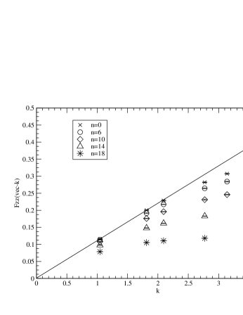
Figure 3: Structure Function $F_{zz}(\vec{k})$ for $N=48$. The line is given by applying the least square fit to data of $n=0$, for which the magnitude of wave vectors is less than $2$.

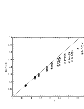
Figure 4: Structure Function $F_{zz}(\vec{k})$ for $N=108$. The line is given by applying the least square fit to data of $n=0$, for which the magnitude of wave vectors is less than $2$.

To check this form, we plot results on $F_{zz}(\vec{k},n)$ as a function of $\mid\vec{k}\mid$ in Figures 3, 4. For $\mid\vec{k}\mid\leq 2$, we can see a linearity of $\mid\vec{k}\mid$ for $N=48$ and $N=108$. This linearity strongly supports that the NG boson dominates in the low energy spectrum. Also we find that $F_{zz}(\vec{k},n)$ depends on $n$. In order to see this $n$-dependence in detail, we plot $F_{zz}(\vec{k},n)$ as a function of $n^{2}$. From these plots we find that $F_{zz}(\vec{k},n)$ are linear functions of $n^{2}$, which are

$$F_{zz}(\vec{k},n)=F_{zz}(\vec{k},0)+g_{zz}(\vec{k})n^{2}\ \ .$$

Next we plot $g_{zz}(\vec{k})$ as a function of $\mid\vec{k}\mid$. By results we guess that this is a linear function of $\mid\vec{k}\mid$. We make the least square fitting on this function using data of $\mid\vec{k}\mid\leq 2$.

$$F_{zz}(\vec{k},n)=\frac{f^{2}}{2}c\mid\vec{k}\mid+(\alpha_{zz}+\beta_{zz}\mid\vec{k}\mid)n^{2}/N^{2}\ \ .$$ (13)

From these figures we obtain for $N=48$ and $N=108$,

$$\frac{f^{2}}{2}c = 0.130\pm 0.004\ ,\ \ \alpha_{zz}=0.26\pm 0.07\ ,$$

$$\ \beta_{zz} = -0.60\pm 0.06\ \ \ {\rm for}\ \ N=48\ \ ,$$

$$\frac{f^{2}}{2}c = 0.126\pm 0.003\ ,\ \ \alpha_{zz}=0.45\pm 0.07\ ,$$

$$\ \ \beta_{zz} = -0.67\pm 0.08\ \ \ {\rm for}\ \ N=108\ \ .$$

A squared error of the expression (13) is calculated by an average of square of differences between data and the expression. The error par one data is $0.0036$ for $N=48$, and $0.0025$ for $N=108$. These small values imply that the function (13) can describe quite well the data.

Next we show results on the structure function on a product of $\hat{S}_{y}(-\vec{k})$ and $\hat{S}_{y}(\vec{k})$, which is defined in a finite size system by

$$F_{yy}(\vec{k},n)=-\langle n+1\mid\hat{S}_{+}(-\vec{k)}\hat{S}_{+}(\vec{k})\mid n-1\rangle/2$$ (14)

$$- \langle n-1\mid\hat{S}_{-}(-\vec{k})\hat{S}_{-}(\vec{k})\mid n+1\rangle/2$$

$$+ \langle n\mid\hat{S}_{-}(-\vec{k})\hat{S}_{+}(\vec{k})\mid n\rangle/2$$

$$+ \langle n\mid\hat{S}_{+}(-\vec{k})\hat{S}_{-}(\vec{k})\mid n\rangle/2\ \ .$$

For $\mid\Psi\rangle$, we have

$$\langle\Psi\mid\hat{S}_{y}(-\vec{k})\hat{S}_{y}(\vec{k})\mid\Psi\rangle=$$ (15)

$$\sum_{n}\{-\langle n+1\mid\hat{S}_{+}(-\vec{k)}\hat{S}_{+}(\vec{k})\mid n-1\rangle/2C^{*}_{n+1}C_{n-1}$$

$$- \langle n-1\mid\hat{S}_{-}(-\vec{k})\hat{S}_{-}(\vec{k})\mid n+1\rangle/2C^{*}_{n-1}C_{n+1}$$

$$+ \langle n\mid\hat{S}_{-}(-\vec{k})\hat{S}_{+}(\vec{k})\mid n\rangle/2C^{*}_{n-1}C_{n+1}$$

$$+ \langle n\mid\hat{S}_{+}(-\vec{k})\hat{S}_{-}(\vec{k})\mid n\rangle/2C^{*}_{n}C_{n}\}$$

$$= \sum_{n}F_{yy}(\vec{k},n)C^{*}_{n}C_{n}$$

$$- \sum_{n}\{\langle n+1\mid\hat{S}_{+}(-\vec{k)}\hat{S}_{+}(\vec{k})\mid n-1\rangle/2(C^{*}_{n+1}C_{n-1}-C^{*}_{n}C_{n})$$

$$+ \langle n-1\mid\hat{S}_{-}(-\vec{k})\hat{S}_{-}(\vec{k})\mid n+1\rangle/2(C^{*}_{n+1}C_{n-1}-C^{*}_{n}C_{n})\}\ \ .$$

This equation shows that if we know coefficients $C_{n}$, we calculate the expectation of $\langle\Psi\mid\hat{S}_{y}(-\vec{k})\hat{S}_{y}(\vec{k})\mid\Psi\rangle$.

If contributions form the NG boson dominate in the structure function for small wave vectors,

$$F_{yy}(\vec{k},n)=\frac{Z^{2}}{2c\mid\vec{k}\mid}+n-{\rm dependent\ terms}\ \ .$$

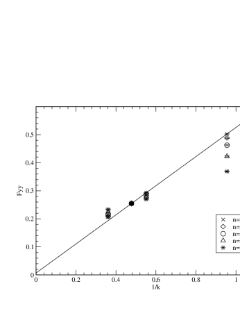
Figure 5: Structure Function $F_{yy}(\vec{k})$ for $N=48$. The line is given by applying the least square fit to data of $n=0$, for which the magnitude of wave vectors is less than $2$.

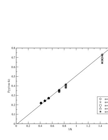
Figure 6: Structure Function $F_{yy}(\vec{k})$ for $N=48$. The line is given by applying the least square fit to data of $n=0$, for which the magnitude of wave vectors is less than $2$.

To check this form, we plot results on $F_{yy}(\vec{k},n)$ as a function of $1/\mid\vec{k}\mid$ in Figures 5, 6. For $\mid\vec{k}\mid\leq 2$, we can see a linearity of $1/\mid\vec{k}\mid$ for $N=48$ and $N=108$. This linearity strongly supports that the NG boson dominates in the low energy spectrum. In order to see this $n$- dependence, we make the same discussion as that for $F_{zz}(\vec{k},n)$. First we plot $F_{yy}(\vec{k},n)$ as a function of $n^{2}$. Then from these plots we find that $F_{yy}(\vec{k},n)$ is a linear function of $n^{2}$, which are

$$F_{yy}(\vec{k},n)=F_{yy}(\vec{k},0)+g_{yy}(\vec{k})n^{2}\ \ .$$

Next we plot $g_{yy}(\vec{k})$ as a function of $1/\mid\vec{k}\mid$. Results suggest that this function is a linear function of $1/\mid\vec{k}\mid$. If we make the least square fitting on this function, we obtain

$$F_{yy}(\vec{k},n)=\frac{Z^{2}}{2c\mid\vec{k}\mid}+(\alpha_{yy}+\beta_{yy}/\mid\vec{k}\mid)n^{2}/N^{2}\ \ .$$ (16)

From figures we obtain for $N=48$ and $N=108$,

$$Z^{2}/2c = 0.458\pm 0.004,\ \alpha_{yy}=0.90\pm 0.04,\$$

$$\beta_{yy} = -1.66\pm 0.06\ \ \ {\rm for}\ N=48\ .$$

$$Z^{2}/2c = 0.439\pm 0.005,\ \alpha_{yy}=0.89\pm 0.12,\$$

$$\beta_{yy} =-1.65\pm 0.15\ \ \ {\rm for}\ N=108\ .$$

A squared error of the expression (16) is calculated by an average of square of differences between data and the expression. The error par one data is $0.0027$ for $N=48$, and $0.0037$ for $N=108$. By these small values it is justified that the function (16) describes the data as well as that for $F_{zz}(\vec{k},n)$.

We make comments on a structure function of a product of $\hat{S}_{y}(-\vec{k})$ and $\hat{S}_{z}(\vec{k})$. In descriptions by the NG boson we have

$$\langle\Psi\mid\hat{S}_{y}(-\vec{k})\hat{S}_{z}(\vec{k})\mid\Psi\rangle=iZf/2\ \ .$$

Also from a commutation of

$$[\hat{S}_{y}(\vec{k}_{1}),\hat{S}_{z}(\vec{k}_{2})]=\frac{i}{\sqrt{N}}\hat{S}_{x}(\vec{k}_{1}+\vec{k}_{2}),$$

we have $Zf=v$. In order to examine this equation, we calculate the structure function in the finite size lattice, which is defined by

$$F_{yz}(\vec{k},n) = \frac{i}{\sqrt{2}}\langle n+1\mid\hat{S}_{+}(\vec{k})\hat{S}_{z}(-\vec{k})\mid n\rangle$$

$$- \frac{i}{\sqrt{2}}\langle n\mid\hat{S}_{-}(\vec{k})\hat{S}_{z}(-\vec{k})\mid n+1\rangle\ \ .$$

We have confirmed numerically that $F_{yz}(\vec{k},n)$’s are independent of wave vectors $\vec{k}$ and their values agree with $v(n)$ within error, although results are omitted.

III.5 Energy for excitations with small wave vectors

In calculations of the structure functions, we do not see the energy $\omega(\vec{k})$ of the excitation, so that we could not determine a value of the velocity $c$, which is defined by $c=\omega(\vec{k})/\mid\vec{k}\mid$. In order to obtain the velocity, we calculate the energy by a following method. If $\mid\vec{k},n\rangle$ is a state of one NG boson with a wave vector $\vec{k}$ and a charge $n$, we have $\hat{H}\mid\vec{k},n\rangle=\mid\vec{k},n\rangle\{\omega(\vec{k})+E(N,n)\}$. Note that $E(N,n)$ is the lowest energy for the charge $n$. It is difficult to get an eigenvalue so that we are contented with an expectation value of the $\hat{H}$, which is given by

$$\omega_{A}(\vec{k})=\langle\vec{k},n\mid\hat{H}\mid\vec{k},n\rangle-E(N,n)\ \ .$$

The results on the structure function imply that the spin operator $\hat{S}_{z}(\vec{k})$ can create a state of one NG-boson with a wave vector $\vec{k}$ from the lowest energy state $\mid n\rangle$. Therefore we can approximate the state of one NG boson by the lowest energy state that is operated by $\hat{S}_{z}(\vec{k})$.

$$\hat{S}_{z}(\vec{k})\mid n\rangle\sim\mid\vec{k},n\rangle A\ .$$

Here $A$ is a constant. If we use this approximation, a calculated energy $\omega_{A}(\vec{k})$ is

$$\omega_{A}(\vec{k}) =\langle\vec{k},n\mid\hat{H}\mid\vec{k},n\rangle-E(n)\ \ ,$$ (17)

$$= A^{2}\langle\vec{k},n\mid\hat{H}\mid\vec{k},n\rangle/(A^{2}\langle\vec{k},n\mid\vec{k},n\rangle)-E(n)\ \ ,$$

$$\sim \langle n\mid\hat{S}_{z}(-\vec{k})\hat{H}\hat{S}_{z}(\vec{k})\mid n\rangle/(\langle n\mid\hat{S}_{z}(-\vec{k})\hat{S}_{z}(\vec{k})\mid n\rangle)$$

$$- E(n)\ \ .$$

Results of calculations of $\omega_{A}(\vec{k})$ are collected in Table 2.

N	n	$(k_{x},k_{y})$	$\omega$	c
48	0	$(\pi/3,0)$	$0.83\pm 0.04$	$0.79\pm 0.04$
48	0	$(\pi/2,-\frac{\pi}{2\sqrt{3}})$	$1.46\pm 0.03$	$0.80\pm 0.03$
48	6	$(\pi/3,0)$	$0.85\pm 0.02$	$0.81\pm 0.02$
48	6	$(\pi/2,-\frac{\pi}{2\sqrt{3}})$	$1.36\pm 0.03$	$0.75\pm 0.02$
48	10	$(\pi/3,0)$	$0.69\pm 0.04$	$0.69\pm 0.04$
48	10	$(\pi/2,-\frac{\pi}{2\sqrt{3}})$	$1.33\pm 0.03$	$0.73\pm 0.03$
108	0	$(\frac{2\pi}{9},0)$	$0.56\pm 0.03$	$0.80\pm 0.04$
108	0	$(\frac{\pi}{3},-\frac{\pi}{3\sqrt{3}})$	$1.01\pm 0.02$	$0.83\pm 0.02$
108	0	$(\frac{4\pi}{9},0)$	$1.16\pm 0.02$	$0.83\pm 0.02$
108	0	$(\frac{5\pi}{9},-\frac{\pi}{3\sqrt{3}})$	$1.40\pm 0.02$	$0.76\pm 0.02$
108	6	$(\frac{2\pi}{9},0)$	$0.58\pm 0.04$	$0.83\pm 0.06$
108	6	$(\frac{\pi}{3},-\frac{\pi}{3\sqrt{3}})$	$1.02\pm 0.03$	$0.84\pm 0.03$
108	6	$(\frac{4\pi}{9},0)$	$1.11\pm 0.03$	$0.80\pm 0.03$
108	6	$(\frac{5\pi}{9},-\frac{\pi}{3\sqrt{3}})$	$1.42\pm 0.03$	$0.77\pm 0.02$
108	10	$(\frac{2\pi}{9},0)$	$0.53\pm 0.03$	$0.76\pm 0.05$
108	10	$(\frac{\pi}{3},-\frac{\pi}{3\sqrt{3}})$	$0.98\pm 0.03$	$0.81\pm 0.03$
108	10	$(\frac{4\pi}{9},0)$	$1.08\pm 0.03$	$0.77\pm 0.03$
108	10	$(\frac{5\pi}{9},-\frac{\pi}{3\sqrt{3}})$	$1.44\pm 0.03$	$0.78\pm 0.03$
108	16	$(\frac{2\pi}{9},0)$	$0.52\pm 0.2$	$0.74\pm 0.04$
108	16	$(\frac{\pi}{3},-\frac{\pi}{3\sqrt{3}})$	$0.94\pm 0.03$	$0.78\pm 0.03$

Table 2: energy of an excited state with a wave vector

For $n=0$, the velocity is a constant for the small wave vector within some error. This value is a little larger than 0.75 that is calculated by the linear spin wave theory. On the $n$-dependence of the velocity we could not make a definite conclusion due to the large error. Here we would like stress that these results are quite non-trivial because calculations on the Hamiltonian are completely independent from those on the structure functions.

IV Summary and discussions

Recent experiments on condensed matters as alkali atoms and superconductors require more complicated macroscopic wave functions, which differ essentially from the simple coherent state. In order to understand phenomena by these wave functions in quantum spin systems, we have made theoretical study on states of the SSB in these systems. In this work we used the VMC method for numerical study. In this method we have to assume that the trial state is close to an exact eigen state of the Hamiltonian. Based on this assumption a study was made for the XY quantum antiferromagnet on the triangular lattice, where the good trail state has been known. Also in order to justify this assumption, we employed the SSS method to calculate the square of the Hamiltonian. By results on the square we confirmed that the trial state was of a high quality.

Our numerical examination has been made on states that become degenerate in a infinitely large lattice, after the confirmation on dominance of a NG boson in low energy excitation. In the examination we calculated the energy, the expectation value of the spin operator and the structure functions of spin by fixing a quantum number, which is a value of the $z$ component of all spins.

Our results on numerical calculation in lattice sizes of 48 and 108 showed that the energy of a small wave vector was linear to a magnitude of the wave vector. In addition it was shown that the expectation values of the operators studied here were linear functions of a square of the quantum number, $n^{2}$. Though in our study this conclusion is limited to the XY model on the triangular lattice, we suppose that the same conclusion can be obtained for other quantum spin models because $n$-dependent terms are restricted partially by algebraic structures as seen in appendix B.

Final comments are made on experimental observations of the $n$-dependent terms. Our results show that for a ground state with $n\ll N$ and a large $N$, one can neglect contributions of $n$-dependent terms. However if a external interaction is the charge operator $\hat{B}=h\hat{Q}$, the ground state is $\mid n*\rangle$, where $n*=h/2d\ N$. For this state there exists a possibility of observing the $n$-dependent terms. More detailed discussion will be made in future works.

Appendix A Appendix A

In this appendix we discuss on the VMC method and the SSS method. A trial state $\mid\Psi\rangle$ is given by the coefficients $c(\{s_{i}\})$ on the basis state, as described in section 2.

$$\mid\Psi\rangle=\sum_{\{s_{i}\}}\mid\{s_{i}\}\rangle c(\{s_{i}\})\ \ .$$

In the VMC method, a probability variable $X$ is a basis state of $\mid\{s_{i}\}\rangle$. A probability $P_{VMC}(X=\{s_{i}\})$ for this variable is defined by

$$P_{VMC}(X=\{s_{i}\})=\mid c(\{s_{i}\})\mid/[\sum_{\{s_{j}\}}\mid c(\{s_{j}\})\mid]\ \ .$$

In a Markov chain Monte Carlo method, what we need is only a ratio of probabilities, $\mid c(\{s_{i}^{\prime}\})\mid/\mid c(\{s_{i}\})\mid$ so that we do not need the normalization factor, which corresponds to the denominator. In this method a expectation value of a operator $\hat{O}$ in the trial state $\mid\Psi\rangle$ is given by

$$\langle\Psi\mid\hat{O}\mid\Psi\rangle/\langle\Psi\mid\Psi\rangle$$

$$= \frac{\sum_{\{s^{\prime}_{i}\}}\sum_{\{s_{j}\}}c^{\dagger}(\{s^{\prime}_{i}\})O_{\{s^{\prime}_{i}\},\{s_{j}\}}c(\{s_{j}\})}{\sum_{\{s_{i}\}}\mid c(\{s_{i}\})\mid^{2}}\ \ ,$$

$$= [\ \sum_{\{s^{\prime}_{i}\}}\sum_{\{s_{j}\}}c^{\dagger}(\{s^{\prime}_{i}\})O_{\{s^{\prime}_{i}\},\{s_{j}\}}c(\{s_{j}\})/\mid c(\{s_{j}\})\mid$$

$$\cdot P_{VMC}(X=\{s_{j}\})\ ]$$

$$/ [\ \sum_{\{s_{i}\}}\mid c(\{s_{i}\})\mid P_{VMC}(X=\{s_{i}\})\ ]\ \ ,$$

where

$$O_{\{s^{\prime}_{i}\},\{s_{j}\}}=\langle\{s^{\prime}_{i}\}\mid\hat{O}\mid\{s_{j}\}\rangle\ \ .$$

Here note that we do not need $\langle\Psi\mid\Psi\rangle=1$ . Actually the trial state we used in this study is not normalized.

While in the SSS method we give a probability variable $X_{\{s_{i}\}}$ to each basis state $\mid\{s_{i}\}\rangle$, whose value is $0$ or $a_{\{s_{i}\}}$. Here $1/a_{\{s_{i}\}}=min(1,\mid c(\{s_{i}\})\mid C)\leq 1$. A probability $P_{SSS}(X_{\{s_{i}\}}=a_{\{s_{i}\}})=1/a_{\{s_{i}\}}$ , while $P_{SSS}(X_{\{s_{i}\}}=0)=1-1/a_{\{s_{i}\}}$. An average of $X_{\{s_{i}\}}$ is 1. We multiply this probability variable $X_{\{s_{i}\}}$ to a coefficient $c(\{s_{i}\})$ and we have $X_{\{s_{i}\}}c(\{s_{i}\})$, that results in 0 or $phase(c(\{s_{i}\}))/C$. Here $phase(x)=x/\mid x\mid$. A state with a nonzero coefficient is called as a sampled state after the multiplication. A value of $C$ determines an average number of sampled states. That is, as $C$ becomes large, this number increases and the statistical error decreases.

We will describe a calculation method for an expectation value of the Hamiltonian squared, $\langle\Psi\mid\hat{H}^{2}\mid\Psi\rangle$. First by the VMC method we make sampling to collect $N_{smpl}$ basis states. Next we operate the Hamiltonian $\hat{H}$ to these sampled states. After the operation, a number $N_{H}$ of the basis states with nonzero coefficients is a few hundred times of $N_{smpl}$. If we operate $\hat{H}$ to $N_{H}$ basis states, we need very huge number of basis states for calculations of its inner product with the trial state $\mid\Psi\rangle$. This huge number makes a calculation difficult due to limited resources of CPU time and computer memory. In order to overcome this difficulty, we employ the SSS method to $N_{H}$ basis states to reduce a number of basis states. After a reduction of the basis states, we operate $\hat{H}$ and calculate its inner product with the trial state $\mid\Psi\rangle$. By repeating these calculations, we make a statistical average for $\langle\Psi\mid\hat{H}^{2}\mid\Psi\rangle$.

Appendix B Appendix B

In this appendix we will present a discussion on $n$ dependence of $v(n)=\langle n+1\mid\hat{S}_{+}(i)\mid n\rangle$. We start from a commutation relation on the spin operator.

$$[\hat{S}_{+}(i),\hat{S}_{-}(j)]=2\delta_{ij}\hat{S}_{z}(i)\ \ .$$

By the state $\mid n\rangle$ we calculate a expectation value of operators in both sides.

$$\langle n\mid[\hat{S}_{+}(i),\hat{S}_{-}(j)]\mid n\rangle=\delta_{ij}\langle n\mid\hat{S}_{z}(i)\mid n\rangle\ \ ,$$

$$\langle n\mid\hat{S}_{+}(i)\hat{S}_{-}(j)\mid n\rangle=\langle n\mid\hat{S}_{+}(i)\mid n-1\rangle\langle n-1\mid\hat{S}_{-}(j)\mid n\rangle\ \$$

$$+\sum_{e}\langle n\mid\hat{S}_{+}(i)\mid n-1,e\rangle\langle n-1,e\mid\hat{S}_{-}(j)\mid n\rangle\ \ .$$

Here $\mid n-1,e\rangle$ denotes an excited state of the charge of $n-1$. We assume that the second term can be neglected as described in Ref.Neuberger . Noting that $\langle n-1\mid\hat{S}_{-}(j)\mid n\rangle=\langle n\mid\hat{S}_{+}(j)\mid n-1\rangle^{\dagger}=v(n-1)^{\dagger}$, we obtain a following relation by making a sum over $i,j$

$$\{v(n-1)\}^{2}-\{v(n)\}^{2}=2n/N^{2}\ \ .$$

Therefore we have

$$\{v(n)\}^{2}=\{v(0)\}^{2}-n(n+1)/N^{2}\ \ .$$ (18)

Here note that $v(n)$ is real as explained in section 3.3.

The above discussion explains well the linear dependence of $\{v(n)\}^{2}$ on $n(n+1)$ which is found in Fig. 2, although decreasing rates differ from the above estimations even for $N=108$. It may imply that it is too rough to neglect contributions from excited states in calculating $\langle n\mid[\hat{S}_{+}(i),\hat{S}_{-}(j)]\mid n\rangle$.

Figure 1: The lowest energy for each n. Errors are small so that we do not plot error bars. The lines are given by applying the least square fit to data.

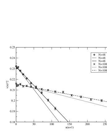
Figure 2: Squares of the expectation values for each n. The bold lines are given by applying the least square fit to data. The slim lines are given by equation (18).

References

• (1) J. Richter, J. Schulenburg and A. Honecker, Quantum Magnetism (Lecture notes in physics 645), edited by U. Schollwöck, J. Richter, D. Farnell and R. Bishop (Springer-Verlag, Berlin, Ger. , 2004).
• (2) A. Auerbach Interacting Elelctrons and Quantum Magnetism (Springer-Verlag, Berlin, Ger. , 1994).
• (3) N. Hatano and M. Suzuki, Quantum Monte Carlo Methods in Condensed Matter Physics, edited by M. Suzuki (World Scientific, Singapore, Singapore, 1993) pp.13.
• (4) H. De Raedt and W. von der Linden, The Monte Carlo Method in Condensed Matter Physics, edited by K. Binder, ( Springer, Berlin, Ger. ,1995 ) pp.249.
• (5) M. Andrews, C. Twonsend, H. Miesner, D. Durfee, D. Kurn and W. Ketterle, Science 275, 637(1997).
• (6) W. Mullin and F. Laloe, Phys.  Rev.  Lett. 104, 150401(2010).
• (7) J. Javanainen and S. Yoo, Phys.  Rev.  Lett. 76, 161(1997).
• (8) M. Iazzi and K. Yuasa, Phy.  Rev.  A 83, 033611(2011).
• (9) Y. Nakamura, C. Chen and J. Tsai, Phys.  Rev.  Lett. 79, 2328(1996).
• (10) S. Singamaneni, V. Bliznyuk, C. Binek and E. Tsymbal, Journal of Materials Chemistry 21, 16819 (2011).
• (11) T. Munehisa and Y. Munehisa, J.  Phys. : Condens. Matter 21, 236008(2007).
• (12) T. Munehisa and Y. Munehisa, arXiv:1008.1612[cond-mat.stat-mech]
• (13) A. Sandvik and C. Hamer, Phys.  Rev.  B 60, 6588 (1999).
• (14) P. Tomczak and J. Richter, J.  Phys.  A:  Math.  Gen. 34, L461 (2001).
• (15) R. Singh and D. Huse, Phys.  Rev.  Lett. 68, 1766(1992).
• (16) L. Capriotti, A. Trumper and S. Sorella, Phys.  Rev.  Lett. 82, 3899(1999).
• (17) A. Trumper, L. Capriotti, S. Sorella, Canadian Journal of Physics 79, 1537 (2001).
• (18) Z. Liu and E. Manousakis, Phys.  Rev.  B 40, 11437 (1989).
• (19) T. Munehisa and Y. Munehisa, J. Phys.  Soc.  Japan 72, 2759(2003).
• (20) T. Munehisa and Y. Munehisa, J.  Phys.  Soc.  Japan 73, 340(2004).
• (21) T. Munehisa and Y. Munehisa J.  Phys.  Soc.  Japan 73, 2245(2004).
• (22) T. Munehisa and Y. Munehisa, arXiv:0403626[cond-mat.stat-mech].
• (23) T. Munehisa and Y. Munehisa, J.  Phys.  Condens.  Matter 18, 2327(2006).
• (24) T. Munehisa and Y. Munehisa, J.  Phys.  Condens.  Matter 19, 196202(2007).
• (25) W. Zheng, R. McKenzie and R. Singh, Phys. Rev. B 59, 14367(1999).
• (26) A. Trumper, L. Capriotti and S. Sorella, Phys. Rev. B 61, 11529(2000).
• (27) L. Arrachea, L. Capriotti and S. Sorella, Phys. Rev. B 69, 224414(2004).
• (28) S. Yunoki and S. Sorella, Phys.  Rev.  B 74 014408(2006).
• (29) D. Ceperley and M. Kalos, Monte Carlo Methods in Statistical Physics, edited by K. Binder (Springer-Verlag, Berlin, Ger. , 1986) pp.145.
• (30) H. Neuberger and Y. Ziman, Phys.  Rev.  B 39, 2608(1989).
• (31) F. Jiang, Phys. Rev. B 83, 024419 (2011).
• (32) F. Jiang and U. Wiese, Phys.  Rev.  B 83, 155120 (2011).
• (33) M. Gross, E. Sanchez-Velasco, and E. Siggia, Phys.  Rev.  B 40, 11328 (1989).
Refer to caption