Photometric properties and luminosity function of nearby massive early-type galaxies

Abstract

We perform photometric analyses for a bright early-type galaxy (ETG) sample with 2949 galaxies ($M_{\rm r}<-22.5$ mag) in the redshift range of 0.05 to 0.15, drawn from the SDSS DR7 with morphological classification from Galaxy Zoo 1. We measure the Petrosian and isophotal magnitudes, as well as the corresponding half-light radius for each galaxy. We find that for brightest galaxies ($M_{\rm r}<-23$ mag), our Petrosian magnitudes, and isophotal magnitudes to 25 ${\rm mag/arcsec^{2}}$ and 1% of the sky brightness are on average 0.16 mag, 0.20 mag, and 0.26 mag brighter than the SDSS Petrosian values, respectively. In the first case the underestimations are caused by overestimations in the sky background by the SDSS PHOTO algorithm, while the latter two are also due to deeper photometry. Similarly, the typical half-light radii ($r_{50}$) measured by the SDSS algorithm are smaller than our measurements. As a result, the bright-end of the $r$-band luminosity function is found to decline more slowly than previous works. Our measured luminosity densities at the bright end are more than one order of magnitude higher than those of Blanton et al. (2003), and the stellar mass densities at $M_{\ast}\sim 5\times 10^{11}M_{\odot}$ and $M_{\ast}\sim 10^{12}M_{\odot}$ are a few tenths and a factor of few higher than those of Bernardi et al. (2010). These results may significantly alleviate the tension in the assembly of massive galaxies between observations and predictions of the hierarchical structure formation model.

1 INTRODUCTION

The properties of nearby early type galaxies (ETGs), especially the brightest ones, offer important clues to understanding the cosmic assembly history of massive galaxies. In terms of their morphologies, colors, stellar population content and scaling relations, ETGs appear to be relatively simple systems compared with spirals and other galaxies. There are, however, a lot of renewed interests in their dynamical properties, particularly from the recent integral field unit surveys (e.g. Emsellem et al. 2007; Brough et al. 2010; Cappellari et al. 2012). There is also a debate on their stellar mass assembly processes (Renzini 2006; Scarlata et al. 2007), and so the understanding of ETGs remains a particularly interesting issue.

In the past two decades, the concept of “downsizing” (Cowie et al. 1996; Gavazzi & Scodeggio 1996; Fontanot et al. 2009) for galaxy formation has been widely discussed. According to this scenario, the epoch of star formation in ETGs depends on the galaxy mass, namely, the most massive ETGs formed their stars on a shorter time scale and at earlier times. Furthermore, large ground-based and space-based imaging and spectroscopic surveys at low and high redshifts found that the mass function shows a weak evolution for massive ETGs since redshift $\sim 1$ (e.g. Cimatti et al. 2006; Scarlata et al. 2007; Cool et al. 2008; Cimatti 2009; Vulcani et al. 2011). In contrast, theory predicts that the typical stellar mass of most massive ETGs increases by a factor of 2-4 since redshift one (see De Lucia & Blaizot 2007; Tonini et al. 2012).

The size evolution for ETGs has also been the topic of many recent studies. It has been shown that the massive and quiescent ETGs with stellar mass $M_{\ast}\geq 10^{11}M_{\odot}$ at high redshift are more compact with effective radii a factor of $\sim$ 3-5 smaller than the present-day ETGs with similar stellar masses, but the stellar masses increase by a factor of $\sim$ 2 since redshift 2 (e.g. Daddi et al. 2005; Trujillo et al. 2006; van Dokkum et al. 2008). A popular explanation for the evolution of massive ETGs is minor dry mergers, although additional physical mechanisms may be required (e.g. Cimatti et al. 2008; Bezanson et al. 2009; van Dokkum et al. 2010; Bruce et al. 2012 and McLure et al. 2012). Moreoever, Valentinuzzi et al. (2010) and Poggianti et al. (2013) found compact (superdense) massive ETGs in the local universe that have sizes comparable to high-z massive galaxies. They argued that the evolution in the median and average size is mild from high to low redshift for galaxies with stellar masses $3\times 10^{10}M_{\odot}<M_{\ast}<4\times 10^{11}M_{\odot}$, whereas the evolution can still be substantial for ETGs more massive than $4\times 10^{11}M_{\odot}$. It should also be noted that such studies have not focused on the evolution of ETGs at the high mass end with $M_{\ast}\geq 10^{12}M_{\odot}$. As pointed out by Naab (2012), the most massive ETGs or their progenitors start forming their stars at redshift $\sim 6$ or even earlier and these high redshift galaxies are just the cores of their local counterparts. The assembly at later times may be inside out by accretion of stellar mass in the outskirts of these galaxies. However, the mass assembly history of most massive ETGs is not yet completely clear: the current $\Lambda$CDM model cannot reproduce the stellar age, metallicity and color evolution simultaneously (Tonini et al. 2012; De Lucia & Borgani 2012).

To understand the mass and size evolution, accurate photometry for massive ETGs is an essential first step. Bright galaxies tend to be located in crowded environments or have extended stellar halos. Inadequate masking of their neighbors or extended halos can result in an overestimate of the sky background, leading to an underestimate of their luminosity and size. Indeed a number of investigators have noted that the SDSS photometric reduction systematically underestimates the luminosities and half-light radii for bright ETGs (see Aihara et al. 2011 for the SDSS DR8 release and DR7 documentation). For the SDSS DR8, a more sophisticated sky background subtraction algorithm has been adopted and significant improvements were achieved, but some problems still persist (see §4.1). On the other hand, the surface brightness distribution of most massive ETGs cannot be fit well by a simple model such as the commonly used Sérsic (1963) law, which can also lead to an underestimate of the luminosities. Graham et al. (2005) carefully investigated the deficiency of Petrosian (1976) system to quantify galaxy luminosity and size. They find that the Petrosian magnitude and size commonly used by studies based on SDSS strongly depend on the surface brightness profile. For example, the flux deficiency can be as large as 0.5 mag for a galaxy with $r^{1/8}$ surface brightness profile. To avoid underestimating the luminosities of the brightest cluster galaxies (BCGs), von der Linden et al. (2007) used isophotal photometry to 23 ${\rm mag/arcsec^{2}}$ in the $r$-band, rather than the Petrosian magnitude. Therefore, aperture photometry offers a viable alternative to describe the photometric properties of ETGs.

Underestimating the luminosities of luminous ETGs will lead to an underestimate of the stellar mass density at the bright end. Using their own sky background subtraction algorithm (cmodel) and stellar mass estimation, Bernardi et al. (2010) found a higher number of very massive galaxies than previous works. The excess can be up to a factor of $\sim$ 10 when the stellar mass $M_{\ast}$ is larger than $5\times 10^{11}M_{\odot}$, which is highly significant.

In this work, we perform accurate photometry for a complete sample of nearby bright early-type galaxies with $M_{\rm r}<-22.5$ mag and $M_{\ast}>10^{11}M_{\odot}$. The morphologies of these galaxies are taken from the Galaxy Zoo project which classified nearly 900,000 SDSS galaxies (Lintott et al. 2011). We perform our own sky background subtraction, which leads to much more accurate photometry of ETGs. We then compare the luminosities and sizes measured by different methods and investigate the luminosity function as well as the stellar mass density for the bright ETGs.

The structure of this paper is as follows. In §2 and §3 we describe the sample selection and data reduction for our bright ETGs. In §4, we compare our measured luminosities and sizes of bright ETGs with the SDSS Petrosian magnitudes and sizes, and present the results of the $r$-band luminosity function and the stellar mass density. We finish the paper with a summary in §5. In this paper, we adopt a Hubble constant of $H_{\rm 0}=70\,{\rm km\,s^{-1}Mpc^{-1}}$, matter density parameter $\Omega_{m}=0.3$ and cosmological constant $\Omega_{\Lambda}=0.7$.

2 SAMPLE

Our bright early type galaxy (ETG) sample is drawn from the morphological catalogue of Galaxy Zoo 1 (Lintott et al. 2011). The Galaxy Zoo 1 project performed visual morphological classifications for nearly 900,000 galaxies from the Sloan Digital Sky Survey (SDSS, York et al. 2000), in which 667,945 galaxies are from the Main Galaxy Sample of SDSS (MGS, Strauss et al. 2002). The MGS includes galaxies with $r$-band Petrosian magnitude $r\leq 17.77$ and $r$-band Petrosian half-light surface brightness $\mu_{50}\leq 24.5$ mag/arcsec². All 667,945 galaxies from the MGS have spectroscopic redshift in the range of $0.001<z<0.25$ and u, g, r, i, z band photometry based on SDSS DR7 (Lintott et al. 2011).

Given that the SDSS spectroscopy survey is incomplete for bright galaxies with redshift less than 0.05 (Stoughton et al. 2002; Strauss et al. 2002; Schawinski et al. 2007; Kaviraj et al. 2007) and reliable photometric analyses with high signal to noise (S/N) ratios can only be performed for galaxies with $r\leq 16$ mag (Fukugita et al. 2007), we constrain our bright ETG sample to $z>0.05$ and $r<16$ mag. Since we are only concerned with the photometric properties of the luminous ETGs, we further restrict our sample to bright ETGs with $M_{\rm r}<-22.5$ mag. The Petrosian absolute magnitudes, $M_{\rm r}$, are calculated using the equation $M_{\rm r}=m_{\rm r}-5\log(D_{\rm L}/10\,{\rm pc})-A-k$, where $D_{\rm L}$ is the luminosity distance, $A$ is the Galactic extinction obtained from the photometric catalogue of SDSS DR7 and $k$ is the k-correction derived using the IDL KCORRECT algorithm of Blanton et al. (2007). Finally there are 7930 bright ETGs in the redshift range of $0.05<z<0.15$ and $M_{\rm r}<-22.5$ mag.

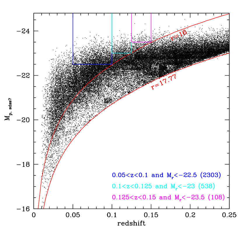
Figure 1: Three volume-limited subsamples selected from Galaxy Zoo 1 early-type galaxies in the redshift vs. absolute Petrosian magnitude plane in the $r$-band of SDSS DR7, shown in blue, cyan and magenta boxes, respectively. The total number of galaxies is 2949 ETGs. The red lines show the observed flux limits at $r=16$ mag and 17.77 mag, respectively. The number of early-type galaxies in each subsample within the redshift range and lower luminosity limit are shown in the bottom right.

We further divide this sample into three volume-limited subsamples with 2303 ETGs in the redshift ranges of $0.05<z<0.1$ for $M_{\rm r}<-22.5$ mag, 538 ETGs with $0.1<z<0.125$ for $M_{\rm r}<-23$ mag and 108 ETGs with $0.125<z<0.15$ for $M_{\rm r}<-23.5$ mag, as shown in Fig. 1. Then we perform $<V/V_{\rm max}>$ test (Schmidt 1968) for these subsamples. The average value $<V/V_{\rm max}>$ are 0.51, 0.50 and 0.51 for the three subsamples, respectively, which indicates that all the three subsamples are spatially homogeneous. The photometric analysis in this work is based on these three subsamples. In total, there are 2949 ETGs brighter than $-$22.5 mag, among which 1053 ETGs are brighter than $-$23 mag. Fig. 2 shows the spatial distribution of our sample galaxies on the sky in Galactic coordinates: the total area is 9055 degree², corresponding to 22% of the whole sky. Fig. 3 presents the histograms showing the distributions of apparent magnitude and spectroscopic redshift for 2949 early-type galaxies. The median Petrosian magnitude is 15.37 mag and median redshift is 0.087, respectively.

In order to verify the early-type morphology of our sample galaxies, we visually inspected the SDSS $r$-band images for all 2949 galaxies. In addition, we also checked other commonly used classification criteria for early-type galaxies. All our sample galaxies have $g-r>0.7$ (e.g. Blanton et al. 2003; Shen et al. 2003), and most (94%) have concentration index $C_{r}=r_{90}/r_{50}$ larger than 2.86 (Bernardi et al. 2010), where $r_{90}$ and $r_{50}$ are the radii containing 90% and 50% of Petrosian flux. Therefore, our selected sample galaxies are all ETGs.

3 DATA REDUCTION

3.1 Estimation of the Sky Background

The corrected frame fpC-images in the $r$-band for our sample galaxies are directly obtained from the SDSS DR7 Data Archive Server. The images have been pre-processed by the SDSS photometric pipeline (PHOTO), which includes bias subtraction, flat-fielding and bad pixels correction (cosmic rays removal, bad columns and bleed trails). In order to obtain the SDSS photometric flux calibration information during observations, such as the photometric zeropoint $a$, the first-order extinction coefficient $k$ and the airmass $X$, we also downloaded the calibrated field statistic file, named as tsField from the archive.

As mentioned in §1, the SDSS photometric reduction systematically underestimates the luminosities and half-light radii for bright ETGs, which is mainly caused by inadequate masking of their neighbors or extended stellar halos (Aihara et al. 2011), leading to an overestimate of the sky background. In this work we perform the masking more carefully and estimate the sky background model following Liu et al. (2008), which has been successfully used to measure the luminosities and half-light radii for the brightest cluster galaxies (BCGs) that are located in crowded fields and usually have extended faint stellar halos.

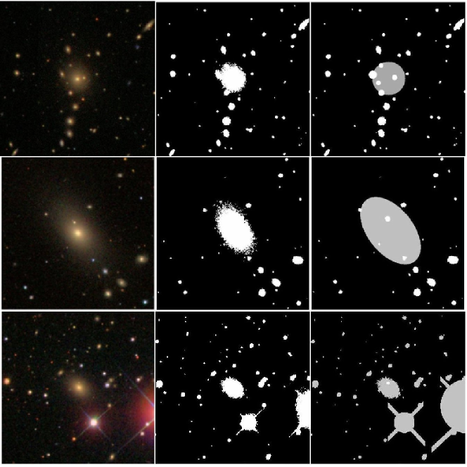
Figure 4: Examples of objects that cannot be masked well by the automatic algorithm of SExtractor. The left panels show examples of color images of ETGs in a crowded field (top row), with extended stellar halo (middle row), and with nearby contaminated stars (bottom row). The middle and right columns show the corresponding masked images generated by SExtractor and by hand. The white areas indicate masked regions.

In the following, we outline our sky background subtraction approach. In order to obtain the sky background, we first masked out all objects detected by SExtractor (Bertin & Arounts 1996) in the corrected frames with $2048\times 1489$ pixels ($13\arcmin.5\times 9\arcmin.8$). We then carefully checked each frame by eye to make sure that the wings of bright stars or the faint stellar halos of galaxies have been properly masked. As expected, we find that the automatic algorithm of SExtractor does not work well for about 24% ETGs brighter than $-$22.5 mag and 33% ETGs brighter than $-$23 mag, which mostly include ETGs residing in crowded fields, having extended stellar halos or are close to foreground bright stars. For the 2949 ETGs brighter than $-$22.5 mag, the percentages of these objects are about 13%, 7%, 4%, respectively. For the 1053 ETGs brighter than $-$23 mag, the percentages are even higher, about 18%, 10%, 5%, respectively. For these ETGs, we modify the mask images manually. For comparison, Fig. 4 shows three cases (top, middle and bottom rows) between the masked images generated by the automatic algorithm of SExtractor (middle panels) and those by hand (right panels). The left panels of Fig. 4 show the original true color images for the example galaxies. The top row shows a galaxy in a crowded field. From the top middle panel, it can be seen that SExtractor cannot separate the target galaxy from its neighbors well. Therefore we manually flag the nearby objects with circles that are large enough to cover the objects completely, as shown in the top right panel. The second row shows a bright ETG with an extended stellar halo. From the middle panel, it is clear that the flagged area generated by SExtractor is not big enough to cover the whole stellar halo. Hence, the stellar halo would be considered as the background and subtracted from the galaxy itself, leading to underestimates of the luminosity and half-light radius of the galaxy. Following the shape of the target ETG, we use an ellipse to mask the entire stellar envelope, as shown in the middle right panel. SExtractor also cannot handle well galaxies surrounded by bright foreground stars, especially those with diffractive spikes (bottom panels). Therefore, we use long rectangles to mask the star spikes (bottom right). The masked images generated manually can provide not only more accurate sky background images but also good masks for the surface photometry (see §4).

To increase the valid area of the sky background subtraction, we smooth the sky background only image with a median filter of $51\times 51$ pixels. This filter size is selected to be larger than the sizes of most objects in the frame but still sufficiently small so that the variation of the sky background within the region is still reproduced (i.e., not smoothed out). After the median filtering is performed, masked regions smaller than the median box filter are replaced with the surrounding sky background, whereas part of the masked regions larger than the median box filter remain flagged. With the small field of view ($13\arcmin.5\times 9\arcmin.8$), the filtered sky background image is fitted with a two-dimensional first-order Legendre polynomial (i.e., $z=a+b*x+c*y$) using the IRAF/IMSURFIT task. The sky background map is typically tilted with a spatial variation of $\sim 1-2$ ADU across the whole frame (Liu et al. 2008). We subtract this sky background model from the initial fpC-image to obtain the sky-corrected frame. The blank regions in the sky-subtracted frame follow Gaussian distributions with means close to zero and standard deviations of several ADU, which is consistent with Liu et al. (2008). After the sky subtraction, we trim both the sky-subtracted frame and the mask image to $501\times 501$ pixels centered on the galaxy of interests. The trimmed mask image with the target galaxy un-flagged will be used to probe the masked regions in the isophote fitting.

3.2 Isophotal Photometry

After the sky background subtraction, we perform surface photometry for our bright ETGs in order to estimate the luminosities and sizes of sample galaxies. As is well known, the Petrosian magnitude and Petrosian size are most commonly used to describe the galaxy flux and half-light radius for the analyses based on SDSS database, because they do not depend on the model fitting to galaxies. The Petrosian radius $r_{\rm p}$ is defined as the radius $r$ at which the ratio of the local surface brightness averaged over an annulus between $0.8r$ and $1.25r$ to the mean surface brightness within $r$ equals to 0.2 and the Petrosian magnitude is the integrated flux within $2r_{\rm p}$ (Petrosian 1976). However, the Petrosian magnitude misses the light outside $2r_{\rm p}$ (Petrosian aperture) because of its dependence on the surface brightness profile of galaxies (Graham et al. 2005), which leads to underestimates of the fluxes and sizes for galaxies with extended stellar halos. In this work, we will measure not only the Petrosian magnitude and Petrosian half-light radius, but also the isophotal magnitude and half-light radius to deeper isophote limits at 25 ${\rm mag/arcsec^{2}}$ and 1% of sky brightness, corresponding to $\sim$ 26 ${\rm mag/arcsec^{2}}$ in most cases (Bernardi et al. 2007).

We perform the surface photometry analysis following Wu et al. (2005) and Liu et al. (2008). The procedures are briefly described below. First, we use ISOPHOTE/ELLIPSE task in IRAF to fit each of the trimmed sky-subtracted images excluding the masked regions in the fitting. The surface brightness of the target galaxy is fitted by a series of elliptical annuli in a logarithmic step of 0.1 along the semi-major axis. The annuli chosen in the outer parts of image is larger, which can suppress the shot noise in the outer regions where the signal to noise ratio (S/N) is much lower. The output of ISOPHOTE/ELLIPSE is the mean intensity in each isophote annulus. Then we integrate the surface brightness profile to isophotal limits of 25 ${\rm mag/arcsec^{2}}$ or 1% of sky brightness to obtain the apparent magnitudes and half-light radius $r_{50}$. We also measure the Petrosian magnitudes and $r_{50}$ based on our sky background subtracted images. In our analysis, the equivalent radius $\sqrt{ab}$ of an ellipse is used for all the radial profiles, where $a$ and $b$ are the semi-major and semi-minor radii of the ellipse. The cosmological dimming is also taken into account for the surface brightness profiles. The observational errors in the surface brightness profile include random errors (e.g., the shot noise of the object and sky background, readout noise and noise contributed by data reduction) and the error from sky background subtraction.

4 RESULTS

4.1 Luminosities of bright ETGs in the local universe

The SDSS database provides the largest galaxy sample with both photometric and spectroscopic information in the local universe. However, the underestimation of the luminosities and sizes for the bright ETGs prevents us from correctly understanding their properties and assembly history.

For brevity in later discussions, we define

$$\begin{array}[]{l}\displaystyle{\Delta m_{\rm p}}=m_{\rm p,\,sdss7}-m_{\rm p},\\ \displaystyle{\Delta m_{\rm 25}}=m_{\rm p,\,sdss7}-m_{25},\\ \displaystyle{\Delta m_{\rm 1\%}}=m_{\rm p,\,sdss7}-m_{1\%},\end{array}$$ (1)

where $m_{\rm p}$, $m_{25}$ and $m_{1\%}$ are our measured Petrosian magnitude, isophotal magnitudes with surface brightness measured to 25 mag/arcsec² and 1% of sky brightness, and $m_{\rm p,\,sdss7}$ is the Petrosian magnitude from the SDSS DR7 pipeline in the $r$-band.

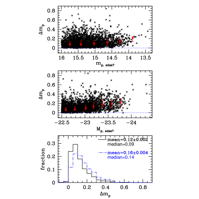
Figure 5: The difference ${\Delta m_{\rm p}}$ between the SDSS Petrosian magnitude and our measured Petrosian magnitude as a function of the SDSS apparent Petrosian magnitude $m_{\rm p,\,sdss7}$ (top panel) and Petrosian absolute magnitude $M_{\rm p,\,sdss7}$ (middle panel). The red data points with error bars are the median, lower (25 per cent) and upper (75 per cent) quartiles for binned galaxies. The bin width is 0.4 mag for the apparent Petrosian magnitude except the last bin which has a width of 0.6 mag to include all the remaining objects (top panel); the bin width is 0.2 mag for the absolute magnitude except the last bin which has a width of 0.7 mag to include all the remaining objects (middle panel). The medians shown in red points are 0.081, 0.081, 0.098, 0.114, 0.145, 0.216 mag in top panel, and 0.065, 0.078, 0.101, 0.138, 0.179, 0.188, 0.225 mag in middle panel. The bottom panel shows the histograms of the magnitude difference with the mean and median values indicated in the top right, as black solid line for galaxies with $M_{\rm p,\,sdss7}<-$22.5 mag and blue dot dashed line for galaxies with $M_{\rm p,\,sdss7}<-$23 mag.

The top and middle panels in Fig. 5 show ${\Delta m_{\rm p}}$ (defined eq. 1) as a function of the SDSS Petrosian apparent and absolute magnitudes, respectively, while the bottom panel shows the histogram of ${\Delta m_{\rm p}}$. Clearly for more luminous ETGs, the luminosity difference between the SDSS and our measurements is larger. The mean and median values of the luminosity differences are 0.16 mag and 0.14 mag, respectively. It shows that the algorithm used in the SDSS DR7 has systematically overestimated the sky background for bright ETGs, leading to underestimates in the luminosities of bright ETGs, especially for the brightest ones.

Addressing the same issue, in the SDSS DR8, Aihara et. al. (2011) have re-processed all SDSS imaging data using a more sophisticated sky background subtraction algorithm and obtained significant improvement. The left and right panels of Fig. 6 are histograms of luminosity difference between the SDSS DR8 and SDSS DR7, and between our measurements and SDSS DR8, respectively. We can see that the median values of luminosity difference for these two cases are $-$0.05 mag and $-$0.08 mag, and the mean values are about $-$0.04 mag and $-$0.12 mag, respectively. The new algorithm on sky background subtraction used in the SDSS DR8 has indeed improved the photometric measurement (the mean shift is about 0.04 mag). However, compared to our study it still underestimates the luminosities by about 0.12 mag on average for bright ETGs. We carefully checked each image with very large luminosity differences between the SDSS DR8 and our measurements. We find that most of these galaxies reside in crowded fields or have very extended faint stellar halos, and so the SDSS DR8 treatment of the sky background issue is incomplete.

Liu et al. (2008) found that the isophotal magnitudes $m_{25}$ measured to the surface brightness of 25 ${\rm mag/arcsec^{2}}$ are generally larger than the Petrosian values for BCGs. We thus also compare the Petrosian and isophotal magnitudes for our sample ETGs. The top and middle panels of Fig. 7 show ${\Delta m_{\rm 25}}$ (defined in eq. 1), as a function of the SDSS Petrosian apparent and absolute magnitudes, respectively. It is obvious that ${\Delta m_{\rm 25}}$ increases with the apparent and absolute magnitudes of ETGs. For $M_{\rm p,\,sdss7}<-23$ mag, the mean and median differences are 0.20 mag and 0.17 mag, respectively, which are larger than those for ${\Delta m_{\rm p}}$ (0.16 and 0.14 mag, respectively).

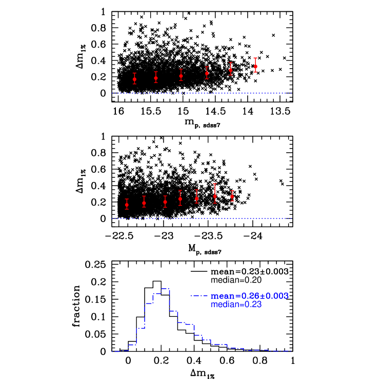
Figure 8: The difference ${\Delta m_{\rm 1\%}}$ between the SDSS Petrosian magnitude and our isophotal magnitude with surface brightness limit at 1% of sky brightness as a function of the SDSS apparent $m_{\rm p,\,sdss7}$ (top panel) and absolute $M_{\rm p,\,sdss7}$ (middle panel) magnitudes. See Fig. 5 for an explanation of the red data points with error bars in the top and middle panels. The medians shown in red points are 0.170, 0.184, 0.209, 0.241, 0.280, 0.326 mag in top panel, and 0.166, 0.131, 0.188, 0.201, 0.237, 0.242, 0.270, 0.267 mag in middle panel. The bottom panel shows the histogram of magnitude difference distribution with the mean and median values indicated in the top right, as black solid line for galaxies with $M_{\rm p,\,sdss7}<-$22.5 mag and blue dot dashed line for galaxies with $M_{\rm p,\,sdss7}<-$23 mag.

Bernardi et al. (2007) investigated the galaxy luminosity by integrating the best-fit model of galaxy surface brightness profile to 1% of sky brightness. The top and middle panels of Fig. 8 show ${\Delta m_{\rm 1\%}}$ (defined in eq. 1) as a function of the SDSS Petrosian apparent and absolute magnitudes, respectively. The same trend is seen: ${\Delta m_{\rm 1\%}}$ increases as ETGs become more luminous. For $M_{\rm p,\,sdss7}<-23$ mag, the mean and median values of ${\Delta m_{\rm 1\%}}$ are 0.26 mag and 0.23 mag, respectively. Note that the photometric limit of 1% sky is $\sim$ 26 ${\rm mag/arcsec^{2}}$, almost one magnitude deeper than 25 ${\rm mag/arcsec^{2}}$.

We further examine the percentage of ETGs with large luminosity difference between the SDSS Petrosian and our measured magnitudes. For the 2949 ETGs brighter than $-22.5$ mag, there are 6%, 12% and 22% ETGs with ${\Delta m_{\rm p}}$, ${\Delta m_{\rm 25}}$ and ${\Delta m_{\rm 1\%}}$ larger than 0.3 mag. For the 1053 ETGs brighter than $-23$ mag, the fractions are even higher, 11%, 19% and 31%, respectively. For more luminous ETGs, the underestimation by the SDSS algorithm is more severe. In addition, the deeper the photometric measurements, the larger the underestimations.

We point out that to the photometric limit of $\sim$ 26 ${\rm mag/arcsec^{2}}$ the light still belongs to galaxies as shown by Tal & van Dokkum (2011). They stacked more than 42000 SDSS images of LRGs (Luminous Red Galaxies), reaching a depth of $\sim$30 ${\rm mag/arcsec^{2}}$, and found that the stellar light out to 100 kpc is physically associated with galaxies, instead of inter-cluster or inter-group light. Our photometric measurement to 1% sky brightness reaches at most 100 kpc (50 kpc on average, see §4.2), and so our measured isophotal light is from ETGs themselves.

4.2 Sizes of bright ETGs in the local universe

Galaxy size is one of the most important parameters of galaxy properties. A reliable determination of the sizes of bright ETGs in the local universe provides the basic calibration for investigating the size evolution, an area of active study in recent years (e.g. Szomoru et al. 2012; McLure et al. 2012; Trujillo 2012). The aforementioned works compare galaxy sizes at high redshift to those of the local universe by Shen et al. (2003) based on the SDSS PHOTO algorithm, who found a power-law relation between the galaxy luminosity and size (Shen et al. 2003). However, if the luminosities of galaxies have been underestimated, galaxy sizes may have been underestimated too. In this section, we will discuss the size difference between the SDSS and our measurements based on different luminosity estimations. For convenience, we define $r_{\rm 50,\,p}$, $r_{\rm 50,\,25}$ and $r_{\rm 50,\,1\%}$ as our Petrosian half-light radius, isophotal half-light radii to 25 mag/arcsec² and 1% of the sky brightness. These values will be compared with $r_{\rm 50,\,sdss7}$, the Petrosian half-light radius from the SDSS DR7 pipeline in the $r$-band.

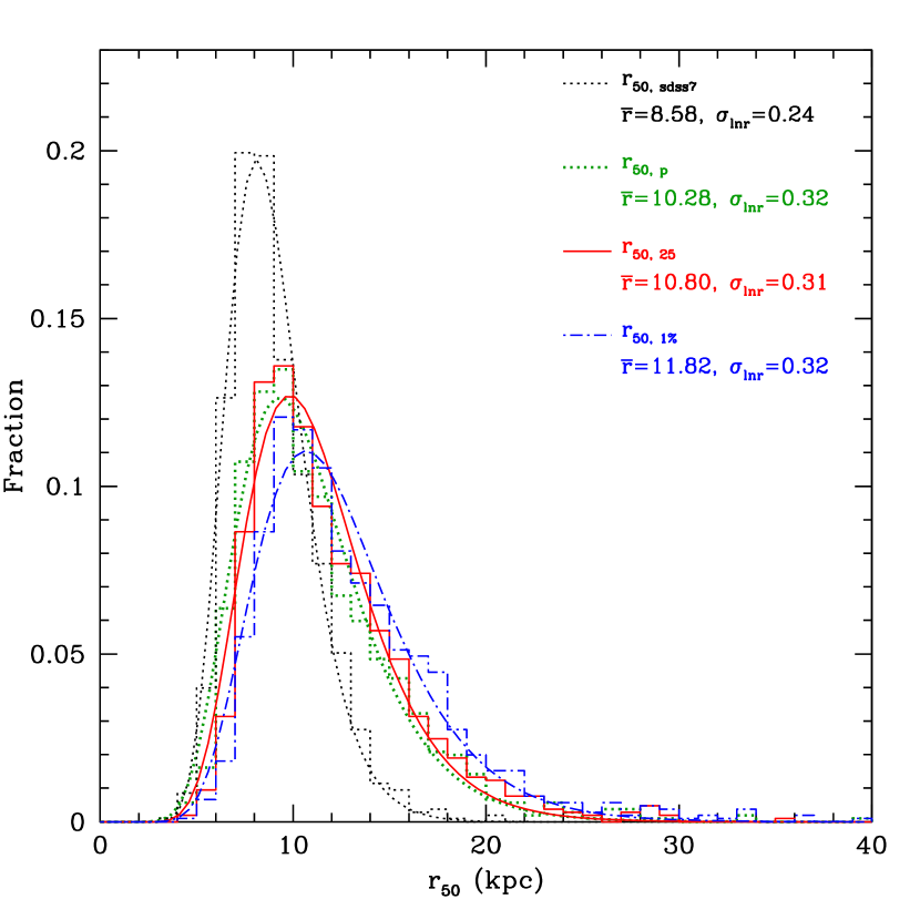
Figure 9: The histograms of half-light radii ($r_{50}$) measured by different photometric methods. The black and green dotted lines represent the Petrosian $r_{50}$ distributions based on SDSS and our own measurements, respectively. While the red solid and blue dot-dashed lines show the $r_{50}$ distributions based on isophotal measurement to 25 ${\rm mag/arcsec^{2}}$ and 1% of sky brightness, respectively. Log-normal (see eq. 2) fits are shown for each distribution with corresponding colors, and the medians and dispersions are shown in the top right.

Fig. 9 presents histograms of the half-light radii measured by different photometric methods. Following Shen et al. (2003), a log-normal function is fitted to the half-light radii distribution. The log-normal function is defined as

$$f(r,\bar{r},\sigma_{\ln{r}})=\frac{1}{\sqrt{2\pi}\sigma_{\ln{r}}}\exp\left[-\frac{\ln^{2}(r/\bar{r})}{2\sigma_{\ln{r}}^{2}}\right]\frac{dr}{r},$$ (2)

which is characterized by the median $\bar{r}$ and the dispersion $\sigma_{\ln{r}}$. We find that the best-fit values for $r_{\rm 50,\,sdss7}$, $r_{\rm 50,\,p}$, $r_{\rm 50,\,25}$, $r_{\rm 50,\,1\%}$ distributions are $\bar{r}=8.58,10.28,10.80,11.82$ kpc and $\sigma_{\ln{r}}=0.24,0.32,0.31,0.32$. From Fig. 9, it can be clearly seen that the largest $r_{\rm 50,\,sdss7}$ value is smaller than 20 kpc, while our measured $r_{\rm 50,\,p}$, $r_{\rm 50,\,25}$ and $r_{\rm 50,\,1\%}$ can be as large as 30 kpc and a large fraction ($\sim$ 27%) of brightest ETGs have sizes larger than 15 kpc. Therefore, the SDSS algorithm has significantly underestimated the real sizes of bright ETGs.

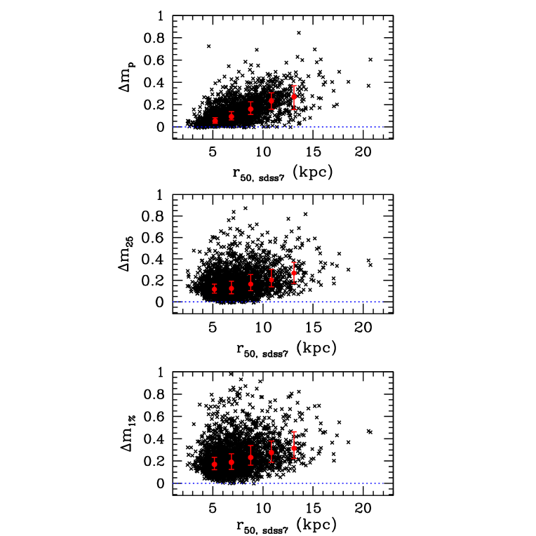
Figure 10: The magnitude differences between the SDSS Petrosian and our measured Petrosian, isophotal magnitudes with surface brightness limits at 25 ${\rm mag/arcsec^{2}}$ and 1% of sky brightness respectively, as a function of the SDSS Petrosian half-light radius $r_{\rm 50,\,sdss7}$. The red data points with error bars are the median, lower (25 per cent) and upper (75 per cent) quartiles for galaxies in bins of width 2 kpc in half-light radius except the first bin which has a width of 4 kpc and the last bin which has a width of 9 kpc to include all the remaining objects. The medians shown in red points are 0.056, 0.093, 0.160, 0.234, 0.270 mag in top panel, and 0.117, 0.125, 0.166, 0.205, 0.269 mag in middle panel, and 0.169, 0.189, 0.232, 0.277, 0.314 mag in bottom panel.

Fig. 10 shows the luminosity differences, ${\Delta m_{\rm p}}$, ${\Delta m_{\rm 25}}$ and ${\Delta m_{\rm 1\%}}$, as a function of $r_{\rm 50,\,sdss7}$ respectively. We can see from Fig. 10 that there is a clear trend that ${\Delta m_{\rm 1\%}}$ increases as ETGs become larger.

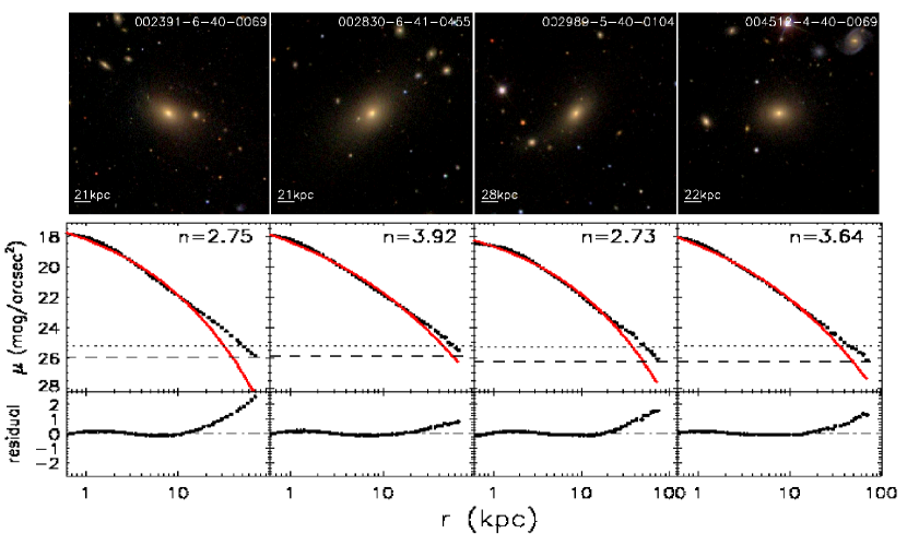
Figure 11: Examples of bright ETGs with extended halos and corresponding surface brightness profiles. The red solid line shows the best fit Sérsic law convolved with the point spread function. The dotted and dashed lines in the middle panels represent the surface brightness of 25 ${\rm mag/arcsec^{2}}$ and 1% of sky brightness respectively. The corresponding Sérsic law index $n$ is shown in the top right of each panel. The bottom panels show the residuals of the observed surface brightness from the Sérsic model.

We further examine the images of the brightest ETGs ($M_{\rm r}<-23$ mag) with differences between the $r_{1\%}$ and the SDSS DR7 measurement larger than 10 kpc and ${\Delta m_{\rm 1\%}}>0.4$ mag. In total, there are 102 such ETGs; 56% ETGs are in crowded field, 26% have extended stellar halos and the remaining 18% are contaminated by bright nearby stars. Fig. 11 represents the ETGs with extended stellar halos (top panels) and corresponding surface brightness profiles (middle panels) and the residuals from Sérsic models (bottom panels). It is obvious from Fig. 11 that the bright ETGs with such very extended stellar halos could not be fitted well by a single Sérsic model.

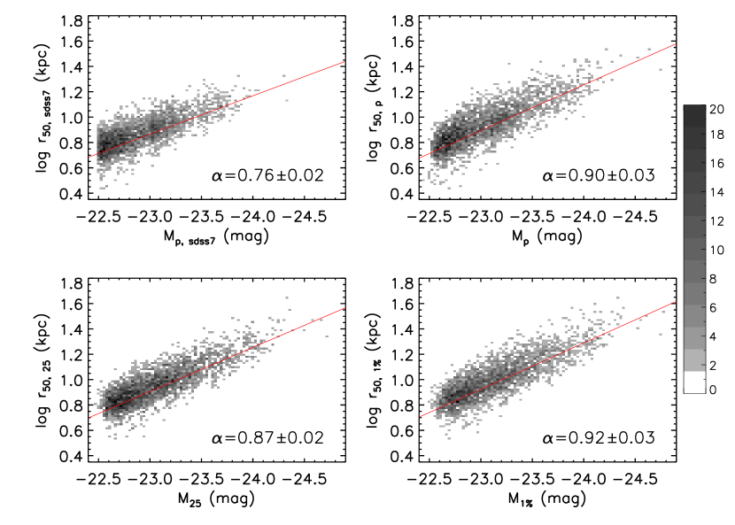
Figure 12: The grayscale representation of the size-luminosity relation for 2949 bright ETGs. The four absolute magnitudes used are the SDSS Petrosian magnitude (top left), our own Petrosian magnitude (top right), and aperture magnitudes to 25 ${\rm mag/arcsec^{2}}$ (bottom left) and 1% of sky brightness (bottom right), respectively. The red line in each panel is the best power-law fit for the size-luminosity relation. The power-law index $\alpha$ ($r_{50}\propto L^{\alpha}$) is shown in the bottom right of each panel. The rightmost vertical grayscale bar reflects the corresponding number of galaxies.

Fig. 12 shows the size and luminosity relations measured by different methods. In each panel, we give the best power-law fit slope for the correlations. The top left and right panels are for Petrosian half-light radius with Petrosian absolute magnitude obtained from the SDSS DR7 catalog and measured by us, respectively. The slope in the top right panel ($\alpha=0.90\pm 0.03$) is steeper than that in the top left panel ($\alpha=0.76\pm 0.02$). It indicates that the sky background subtraction for bright ETGs significantly influences the size-luminosity relation. The bottom left and right panels of Fig. 12 show the correlations between the size and isophotal absolute magnitude to 25 ${\rm mag/arcsec^{2}}$ and to 1% of sky brightness, respectively. We can see from the bottom two panels of Fig. 12 that the slope for the correlation between $\log r_{50,1\%}$ and $M_{1\%}$ ($\alpha=0.92\pm 0.03$) is somewhat steeper than the correlation between $\log r_{50,25}$ and $M_{25}$ ($\alpha=0.87\pm 0.02$). These results are consistent with the size-luminosity relation trend for the brightest cluster galaxies (BCGs) obtained by Liu et al. (2008) who found that the power-law slope becomes steeper when the measurement goes deeper (see also Bernardi et al. 2007).

Our derived slope on the $\log r_{50}$ and $M_{\rm r}$ relation for ETGs is much larger than the value 0.67 found by Shen at al. (2003) that is widely adopted by recent works on the size evolution for bright ETGs. If we use our measured sizes of ETGs, the size evolution since redshift 2 will be somewhat larger. However, due to the surface brightness dimming, it may be difficult to perform photometry down to 26 ${\rm mag/arcsec^{2}}$ in the rest-frame $r$-band for ETGs at redshift 2. As a result, we should be more cautious in discussing the size evolution by explicitly taking into account the survey surface brightness limit.

4.3 The bright end of the $r$-band LF and stellar mass density

A basic way to investigate galaxy properties and their evolution is by studying the luminosity function (LF). There are already many LF studies using different samples and approaches at different redshifts (see the recent review paper by Johnston 2011). Given that the luminosities of the brightest galaxies ($-$23.5 mag) have been underestimated (by $\sim$10% to 40%), it is worth revisiting the LF at the bright end in the local universe.

In this work, we construct the galaxy luminosity function at the bright end, utilizing the non-parametric $1/V_{\rm max}$ method (Schmidt 1968; Felten 1976; Eales 1993). Our bright ETG sample includes 2949 galaxies consisting of three subsamples as described in §2, in which we have already discussed the homogeneity for this sample. Briefly, the $1/V_{\rm max}$ is the inverse of the maximum volume, to which the galaxy could have been detected. The LF is obtained by integrating $1/V_{\rm max}$ in different luminosity bins for the whole sample of galaxies. Given that our ETGs contain three subsamples, we calculate the LF in three volumes separately, and then average them to obtain the final LF. In addition, SDSS fiber collisions lead to $\sim 7\%$ incompleteness for the spectroscopic sample (Bernardi et al. 2010), we multiply the $1/V_{\rm max}$ counts by a factor of $1/0.93$ to obtain the final LF.

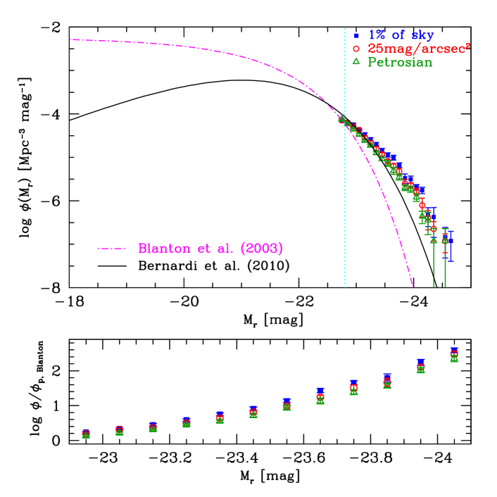
Figure 13: The top panel shows the $r$-band luminosity function at the bright end calculated based on our measured luminosities for 2949 ETGs brighter than $M_{\rm r}<-22.5$ mag. The green triangles, red circles, and blue solid squares represent the LF calculated by using our measured Petrosian magnitude, isophotal magnitudes with surface brightness limits at 25 mag/arcsec² and 1% of sky brightness respectively. The magenta dot-dashed and black solid lines give the fits by Blanton et al. (2003) and Bernardi et al. (2010). The points for objects brighter than the luminosity shown by the cyan dotted line are not affected by photometry. The bottom panel shows the galaxy luminosity density ratios as a function of the $r$-band luminosity. The green triangles, red circles, and blue solid squares show the ratios for our measured Petrosian, isophotal luminosities to 25 mag/arcsec² and 1% of sky brightness to that from Blanton et al. (2003).

The top panel of Fig. 13 shows our $r$-band luminosity function at the bright end. The green triangles, red circles and blue solid squares represent the luminosity function for our measured Petrosian magnitude, isophotal magnitudes measured to the surface brightness of 25 ${\rm mag/arcsec^{2}}$ and 1% of the sky brightness, respectively. For comparison, we also plot the luminosity functions from Blanton et al. (2003) and Bernardi et al. (2010) in the top panel of Fig. 13. Blanton et al. (2003) used a sample of 147,986 galaxies (from SDSS EDR) and the maximum likelihood method to calculate the luminosity function at $z=0.1$. Their sample is much larger, but includes all morphological types. However, at the bright end (e.g. the galaxies brighter than $-$22.5 mag), their galaxies are almost exclusively ETGs. The Petrosian $r$-band luminosity of galaxies in Blanton et al. (2003) are directly obtained from the SDSS catalogue based on the SDSS PHOTO algorithm. Bernardi et al. (2010), on the other hand, used an ETG sample of galaxies selected from $\sim 250000$ SDSS galaxies with $14.5<m_{\rm p,\,sdss}<17.5$ using the concentration index $C_{r}\geq 2.86$, which is a conservative way to select ETGs from SDSS. The luminosities of ETGs in Bernardi et al. (2010) are calculated using the cmodel in the SDSS pipeline with their own sky background subtraction method.

It is clear from the top panel of Fig. 13 that at the bright end ($M_{\rm r}<-22.5$ mag), the slope of the Bernardi et al. (2010)’s LF is shallower than that of Blanton et al. (2003), implying that the luminosity estimation method of Bernardi et al. (2010) is a significant improvement over the SDSS PHOTO algorithm. However, our luminosity function of ETGs at the bright end is even shallower, particularly when we use the photometry to 1% of the sky brightness.

Table 1 lists our measured luminosity densities for the Petrosian magnitudes and isophotal magnitudes to surface brightness of 25 ${\rm mag/arcsec^{2}}$ and 1% of the sky background (denoted by $\phi_{\rm p}$, $\phi_{\rm 25}$ and $\phi_{\rm 1\%}$, respectively) at several $r$-band luminosities. The bottom panel of Fig. 13 shows the ratios of these galaxy luminosity densities to that measured by Blanton et al. (2003), denoted as ${\phi_{\rm p,\,Blanton}}$, as a function of $r$-band luminosities. It is clear that the luminosity density ratios increase with the luminosity of ETGs. For ETGs with $M_{\rm r}=-$23.5 mag, the ratios are $6.7\pm 0.46$, $8.0\pm 0.40$ and $10.5\pm 0.56$, respectively; for ETGs with $M_{\rm r}=-$24 mag, they go up to $153\pm 14$, $197\pm 16$ and $259\pm 22$, respectively. It demonstrates that the luminosity density of the brightest ETG calculated based on the SDSS catalogue has been seriously underestimated. Note that for the three magnitudes $M_{\rm p}$, $M_{\rm 25}$ and $M_{\rm 1\%}$, the number of ETGs brighter than $-$23.5 mag is 347, 385 and 486, while the number of ETGs brighter than $-$24 mag is 41, 56 and 90, and so the number statistics are reasonably good. The underestimates in the luminosity density result in a significant underestimate of the integrated luminosity density. In particular, the integrated luminosity density down to $M_{\rm r}<-22.5$ mag based on our measured $M_{\rm p}$, $M_{25}$, $M_{1\%}$ are about 20%, 40%, 50% higher than that from the SDSS Petrosian luminosity, respectively.

Next we estimate the stellar mass $M_{\ast}$ of the ETGs following Bernardi et al. (2010), utilizing the equation

$$\log\,M_{\ast}/M_{\odot}=1.097(g-r)-0.406-0.4(M_{\rm r}-4.67)-0.19z,$$ (3)

where $M_{\ast}$ is the stellar mass (in solar units), $g-r$ is the rest-frame color, $M_{\rm r}$ is the absolute magnitude, and $z$ is the redshift. This equation has already taken into account the k-correction and evolution correction, and the initial mass function (IMF) is assumed to be of the Chabrier (2003) form (see §2.4 of Bernardi et al. 2010 for more details). The first two terms on the right side of eq. (3) were initially derived by Bell et al. (2003) based on SDSS Petrosian $g-r$ color and $r$-band Petrosian magnigtude, which have been adapted to the Chabrier IMF here. A proper model fitting to colors and magnitudes measured using our photometric methods may give different coefficients in eq. (3). However, to facilitate comparison with the stellar mass function obtained by Bernardi et al. (2010), we use the same equation as their study. Under the assumption that the impact of our photometric algorithm on the $r$-band photometry is the same as that on the $g$-band, we use the SDSS model $g-r$ color as a surrogate of colors measured by our methods. The stellar masses $M_{\ast,\rm\,p}$, $M_{\ast,\,25}$ and $M_{\ast,\,1\%}$ are obtained using our measured luminosities $M_{\rm p}$, $M_{\rm 25}$, $M_{\rm 1\%}$, respectively.

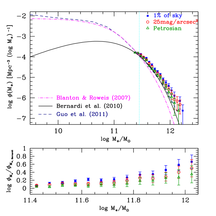
Figure 14: The top panel shows the stellar mass function for massive ETGs. The stellar masses are estimated from our measured Petrosian (green triangles), isophotal luminosities to 25 mag/arcsec² (red circles) and 1% of sky brightness (blue solid squares), respectively. The magenta dot-dashed and black solid lines represent the best-fit stellar mass functions from Blanton & Roweis (2007) and Bernardi et al. (2010), respectively. The navy blue dashed line represents the prediction from the semi-analytic models of the Millennium Simulation of Guo et al. (2011). The points for objects more massive than the stellar mass shown by the cyan dotted line are not affected by the photometry. The bottom panel shows the ratios between our measured stellar mass densities and those of Bernardi et al. (2010) as a function of stellar mass; the symbols are the same as in the top panel.

Table 2 gives the stellar mass densities, $\phi_{M_{\ast},\rm\,p}$, $\phi_{M_{\ast},\,25}$ and $\phi_{M_{\ast},\,1\%}$ at several stellar masses of ETGs for our measured magnitudes. The top panel of Fig. 14 shows the stellar mass function for massive ETGs. We also plot the stellar mass function from Blanton & Roweis (2007) and Bernardi et al. (2010) in the top panel of Fig. 14 for comparison. As can be seen, the slope of our measured stellar mass functions is shallower than those of Bernardi et al. (2010) and Blanton & Roweis (2007). Given that Bernardi et al. (2010) have already compared their stellar mass density with previous observational results, in the bottom panel of Fig. 14 we just compare our result with Bernardi et al. (2010). It shows that the stellar mass densities ratios of our measurements to that of Bernardi et al. (2010), written as $\phi_{M_{*},\rm\,Bernardi}$, as a function of stellar mass. We can see from the bottom panel of Fig. 14 that the ratios are larger for more massive ETGs. The ratios, $\phi_{M_{*},\rm\,p}/\phi_{M_{*},\rm\,Bernardi}$, $\phi_{M_{*},\,25}/\phi_{M_{*},\rm\,Bernardi}$ and $\phi_{M_{*},\,1\%}/\phi_{M_{*},\rm\,Bernardi}$ are 1.2$\pm$0.06, 1.3$\pm$0.07 and 1.6$\pm$0.07 for ETGs with $M_{\ast}\sim 5\times 10^{11}M_{\odot}$; for $M_{\ast}\sim 10^{12}M_{\odot}$, the ratios are even larger, 2.1$\pm$0.40, 2.8$\pm$0.43 and 4.2$\pm$0.58, respectively. Thus, at the high mass end the stellar mass densities have been underestimated by all previous works.

We also plot the predicted stellar mass function by Guo et al. (2011) in the top panel of Fig. 14. Their result is based on the semi-analytic models of the galaxy population using the dark matter only Millennium Simulation. We can see that the high-mass tail of their stellar mass function slightly over-predicts the abundance in Bernardi et al. (2010), but still under-predicts our mass function. We return to this briefly in the next section.

5 SUMMARY

In this work, we performed photometric analyses for a complete and homogeneous bright ETGs sample with 2949 early-type galaxies ($M_{\rm r}<-22.5$ mag) in the redshift range of 0.05 to 0.15, taken from the catalog of SDSS DR7; all these galaxies have morphological classifications from the Galaxy Zoo 1 MGS. Based on our own sky background subtraction method, we measured the Petrosian and isophotal magnitudes, as well as the corresponding half-light radii. Comparing our measured luminosities and sizes to those from SDSS, we find that the SDSS pipeline significantly underestimates the luminosities and sizes for the brightest ETGs, leading to underestimates of the luminosity density and stellar mass density for bright ETGs. Our main results are summarized as follows.

1. We find that for brightest galaxies ($M<-23$ mag), our Petrosian magnitudes, and isophotal magnitudes to 25 ${\rm mag/arcsec^{2}}$ and 1% of the sky brightness are on average 0.16 mag, 0.20 mag, and 0.26 mag brighter than the SDSS Petrosian values, respectively. In the first case the underestimations are due to overestimations in the sky background by the SDSS PHOTO algorithm, while the latter two are also caused by an additional effect of reaching deeper photometry. Such underestimation is more severe as ETGs become more luminous. Our results also demonstrate that as we integrate to deeper surface brightness, we recover more luminosity of galaxies.

2. We also find that the sizes of ETGs (half-light radius $r_{50}$) measured by the SDSS algorithm are smaller than those measured by us. The largest $r_{50}$ of bright ETGs in the SDSS catalogue is $\sim$ 20 kpc, while our measured $r_{50}$ can be as large as 30 kpc and for a large fraction ($\sim$ 27%) of brightest ETGs, $r_{50}$ is larger than 15 kpc. In addition, we find that the slope in the size-luminosity relation at the bright end is much steeper than that found by Shen et al. (2003).

3. Based on our selected complete and homogeneous sample of 2949 bright early-type galaxies, we construct the luminosity function. We find that the LF at the bright end is much shallower than those of Blanton et al. (2003) and Bernardi et al. (2010). The luminosity density at $-$23.5 mag ($-$24 mag) measured in this work is one order (two orders) of magnitude higher than that of Blanton et al. (2003). As a result, the ratios of the integrated luminosity density for bright galaxies ($M_{\rm r}<-22.5$ mag) between those based on our measured $M_{\rm p}$, $M_{25}$, $M_{1\%}$ and the SDSS Petrosian luminosity are 1.2, 1.4 and 1.5, respectively. Similarly, the stellar mass density of ETGs is a few tenths to a factor of few higher than that of Bernardi et al. (2010) for stellar mass from $\sim 5\times 10^{11}M_{\odot}$ to $\sim 10^{12}M_{\odot}$. Therefore, our method recovers substantially more luminosity for bright ETGs, which may alleviate the contradiction between hierarchical galaxy formation theories and current observations.

Our results suggest that very careful photometry needs to be performed to obtain the LF at the bright end which has significant impact on the stellar mass function for massive galaxies. Previous claims that the massive end of the stellar mass function has a weak evolution since redshift $\sim$ 1 in comparison with the Galaxy And Mass Assembly (GAMA) survey (Baldry et al. 2012) may need to be re-examined. Furthermore, semi-analytical models may need to increase their cooling efficiency or decrease the AGN feedback efficiency for massive galaxies in order to match the shallower LF we found here. How does this affect the overall shape of the LF (especially around $L_{*}$) is unclear and warrants further studies. Finally, we notice that recent studies on the environmental dependence of galaxy mass function have suggested that the stellar mass function is much more dependent on local galaxy density than global environments of galaxies and the most massive galaxies are only located in the highest density regions (e.g. Vulcani et al. 2012; Calvi et al. 2013). Given our finding that massive galaxies, which are preferentially found in crowded environments, can be significantly underestimated in their luminosity/mass due to inaccurate photometry, the observed environmental dependence of the high-mass end of mass function may be somehow affected by such photometry issue also. It is worth revisiting this issue in a future work.

Figure 2: The sky coverage for our volume-limited bright early-type galaxies in the Aitoff projection in Galactic coordinates. The total sky coverage is about 9055 degree².

Figure 3: Distributions of the SDSS Petrosian apparent magnitude in the $r$-band (left panel) and redshift (right panel) for 2949 early-type galaxies with $M_{\rm r}<-22.5$ mag. The mean and median values for each distribution are shown in the top left.

Figure 6: The distributions of the difference between the SDSS DR8 and SDSS DR7 Petrosian magnitudes (left panel), and the difference between our measured Petrosian magnitude and the SDSS DR8 (right panel). The mean and median values for each distribution are shown in the top left of the panel.

Figure 7: The difference ${\Delta m_{\rm 25}}$ between the SDSS Petrosian magnitude and our isophotal magnitude to 25 mag/arcsec² as a function of the SDSS apparent $m_{\rm p,\,sdss7}$ (top panel) and absolute $M_{\rm p,\,sdss7}$ (middle panel) isophotal magnitudes. See Fig. 5 for an explanation of the red data points with error bars in the top and middle panels. The medians shown in red points are 0.112, 0.122, 0.151, 0.175, 0.220, 0.278 mag in top panel, and 0.111, 0.131, 0.142, 0.172, 0.180, 0.213, 0.219 mag in middle panel. The bottom panel shows the histogram of magnitude difference distribution with the mean and median values indicated in the top right, as black solid line for galaxies with $M_{\rm p,\,sdss7}<-$22.5 mag and blue dot dashed line for galaxies with $M_{\rm p,\,sdss7}<-$23 mag.

Table 1: Luminosity densities for the Petrosian magnitude ($\phi_{\rm p}$) and isophotal magnitudes to 25 mag/arcsec² ($\phi_{\rm 25}$) and 1% of the sky background ($\phi_{\rm 1\%}$).

$M_{\rm r}$	$\phi_{\rm p}$	$\phi_{\rm 25}$	$\phi_{\rm 1\%}$
(mag)	($10^{-7}$Mpc-3 mag-1)	($10^{-7}$Mpc-3 mag-1)	($10^{-7}$Mpc-3 mag-1)
-22.75	751.745$\pm$34.527	716.908$\pm$33.718	691.239$\pm$33.109
-22.85	588.563$\pm$30.551	634.400$\pm$31.718	645.401$\pm$31.992
-22.95	443.715$\pm$26.526	522.556$\pm$28.787	573.894$\pm$30.168
-23.05	335.537$\pm$23.067	425.380$\pm$25.973	445.300$\pm$26.251
-23.15	244.257$\pm$13.778	286.031$\pm$21.298	340.198$\pm$24.652
-23.25	189.786$\pm$12.098	218.191$\pm$18.601	262.195$\pm$20.391
-23.35	127.568$\pm$9.925	159.517$\pm$15.905	203.522$\pm$17.965
-23.45	92.339$\pm$8.424	118.448$\pm$9.555	146.683$\pm$15.252
-23.55	73.341$\pm$10.785	82.101$\pm$7.963	114.717$\pm$13.132
-23.65	49.505$\pm$8.860	64.004$\pm$7.017	99.011$\pm$12.530
-23.75	35.526$\pm$5.226	47.672$\pm$8.695	66.697$\pm$8.242
-23.85	20.151$\pm$2.954	24.958$\pm$6.438	33.346$\pm$8.371
-23.95	18.670$\pm$2.945	22.846$\pm$3.195	31.383$\pm$5.785
-24.05	12.094$\pm$2.348	16.537$\pm$2.857	20.738$\pm$3.073
-24.15	4.397$\pm$1.394	7.915$\pm$3.681	17.561$\pm$3.025
-24.25	3.582$\pm$1.923	4.075$\pm$1.923	4.776$\pm$2.221
-24.35	1.194$\pm$1.111	2.262$\pm$1.071	4.234$\pm$2.784

Table 2: Stellar mass densities for the Petrosian magnitude ($\phi_{M_{\ast},\rm\,p}$) and isophotal magnitudes to 25 mag/arcsec² ($\phi_{M_{\ast},\rm\,25}$) and 1% of the sky background ($\phi_{M_{\ast},\rm\,1\%}$).

$\log\,M_{\ast}/M_{\odot}$	$\phi_{M_{\ast},\rm\,p}$	$\phi_{M_{\ast},\rm\,25}$	$\phi_{M_{\ast},\rm\,1\%}$
	($10^{-7}$ Mpc${}^{-3}\,{\rm dex}^{-1}$)	($10^{-7}$ Mpc${}^{-3}\,{\rm dex}^{-1}$)	($10^{-7}$ Mpc${}^{-3}\,{\rm dex}^{-1}$)
11.425	1503.490$\pm$69.055	1481.490$\pm$68.547	1437.480$\pm$67.522
11.475	1078.120$\pm$58.476	1239.460$\pm$62.699	1364.140$\pm$65.777
11.525	876.429$\pm$52.723	964.438$\pm$55.307	982.773$\pm$55.830
11.575	685.742$\pm$46.636	722.413$\pm$47.867	880.096$\pm$52.833
11.625	370.374$\pm$34.274	476.719$\pm$38.884	568.396$\pm$42.459
11.675	267.674$\pm$28.369	333.723$\pm$31.676	421.713$\pm$36.572
11.725	202.038$\pm$24.976	201.688$\pm$25.292	260.721$\pm$27.998
11.775	128.623$\pm$19.665	161.351$\pm$22.622	192.372$\pm$24.181
11.825	95.344$\pm$17.390	113.685$\pm$18.989	135.768$\pm$20.758
11.875	55.620$\pm$12.932	62.573$\pm$13.716	80.665$\pm$13.755
11.925	35.519$\pm$9.903	38.211$\pm$8.884	56.210$\pm$13.499
11.975	19.155$\pm$7.968	25.752$\pm$8.448	39.100$\pm$11.500
12.025	11.204$\pm$5.141	15.896$\pm$7.393	23.064$\pm$8.333
12.075	5.627$\pm$4.233	8.355$\pm$5.495	12.604$\pm$6.768

References

- (1) Abazajian K., Adelman-McCarthy, J. K., Agüeros, M. A., et al. 2004, AJ, 128, 502
- (2) Aihara, H., Allende, P. C., An, D., et al. 2011, ApJS, 193, 29
- (3) Baldry, I. K., Driver, S. P., Loveday, J., et al. 2012, MNRAS, 421, 621
- (4) Bell, E. F., McIntosh, D. H., Katz, N., Weinberg, M. D. 2003, ApJS, 149, 289
- (5) Bernardi, M., Hyde, J. B., Sheth, R. K., Miller, C. J., Nichol, R. C. 2007, AJ, 133, 1741
- (6) Bernardi, M., Shankar, F., Hyde, J. B., et al. 2010, MNRAS, 404, 2087
- (7) Bertin, E. & Arnouts, S. 1996, A&A, 117, 393
- (8) Bezanson, R., van Dokkum, P. G., Tal, T., et al. 2009, ApJ, 697, 1290
- (9) Blanton, M. R., Hogg, D. W., Bahcall, N. A., et al. 2003, ApJ, 592, 819
- (10) Blanton, M. R. & Roweis, S. 2007, AJ, 133, 734
- (11) Brough, S., Tran, K.-V, Sharp, R. G., von der Linden, A., Couch, W. J., 2011, MNRAS, 414, L80
- (12) Bruce, V. A., Dunlop, J. S., Cirasuolo, M., et al. 2012, MNRAS, 427, 1666
- (13) Calvi, R., Poggianti, B. M., Vulcani, B., Fasano, G., 2013, MNRAS, in press (arXiv:1304.3124)
- (14) Cappellari, M., McDermid, R. M., Alatalo, K., et al. 2012, MNRAS, in press (arXiv:1208.3523)
- (15) Chabrier G., 2003, ApJ, 586, L133
- (16) Cimatti, A., Daddi, E., Renzini, A. 2006, A&A, 453, L29
- (17) Cimatti, A., Cassata, P., Pozzetti, L., et al. 2008, A&A, 482, 21
- (18) Cimatti, A. 2009, AIPC, 1111, 191
- (19) Cool, R. J., Eisenstein, D. J., Fan, X. H., Fukugita, M., Jiang, L. H., et al. 2008, ApJ, 682, 919
- (20) Cowie, L. L., Songaila, A., Hu, E. M., Cohen, J. G. 1996, AJ, 112, 839
- (21) Daddi, E., Renzini, A., Pirzkal, N., et al. 2005, ApJ, 626, 680
- (22) De Lucia, G. & Blaizot, J. 2007, MNRAS, 375, 2
- (23) De Lucia, G. & Borgani, S. 2012, MNRAS, 426, L61
- (24) Eales, S. 1993, ApJ, 404, 51
- (25) Emsellem, E., Cappellari, M., Krajnović, D., et al. 2007, MNRAS, 379, 401
- (26) Felten, J. E. 1976, ApJ, 207, 700
- (27) Fontanot, F., De Lucia, G., Monaco, P., Somerville, R. S., Santini, P. 2009, MNRAS, 397, 1776
- (28) Fukugita, M., Nakamura, O., Okamura, S., et al. 2007, AJ, 134, 579
- (29) Gavazzi, G., & Scodeggio, M. 1996, A&A, 312, L29
- (30) Graham, A. W., Driver, S. P., Petrosian, V., et al. 2005, AJ, 130, 1535
- (31) Guo, Q., White, S., Bryna-KAlwin, M., et al. 2011, MNRAS, 413, 101
- (32) Johnston, R. 2011, A&ARv, 19, 41
- (33) Kaviraj, S., Schawinski, K., Devriendt, J. E. G., et al. 2007, ApJS, 173, 619
- (34) Lintott, C., Schawinski, K., Bamford, S., et al. 2011, MNRAS, 410, 166
- (35) Liu, F. S., Xia, X. Y., Mao, S. D., Wu, H., Deng, Z. G. 2008, MNRAS, 385, 23
- (36) McLure, R. J., Pearce, H. J., Dunlop, J. S., et al. 2012, MNRAS, in press (arXiv:1205.4058)
- (37) Naab T. 2012, in Proc. of the XXVIII IAU General Assembly, eds. D. Thomas, A. Pasquali; I. Ferreras. Cambridge University Press, in press (arXiv:1211.6892)
- (38) Petrosian, V. 1976, ApJ, 209, L1
- (39) Poggianti, B. M., Calvi, R., Bindoni, D., et al. 2013, ApJ, 762, 77
- (40) Renzini, A. 2006, ARA&A, 44, 141
- (41) Scarlata, C., Carollo, C. M., Lilly, S. J., et al. 2007, ApJS, 172, 494
- (42) Schawinski, K., Kaviraj, S., Khochfar, S., et al. 2007, ApJS, 173, 512
- (43) Schmidt, M. 1968, ApJ, 151, 393
- (44) Sérsic, J. L. 1963, Bol. Asoc. Argent. Astron., 6, 41
- (45) Shen, S., Mo, H. J., White, S. D. M., et al. 2003, MNRAS, 343, 978
- (46) Stoughton, C., Lupton, R. H., Bernardi, M., et al. 2002, AJ, 123, 485
- (47) Strauss, M. A., Weinberg, D. H., Lupton, R. H., et al. 2002, AJ, 124, 1810
- (48) Szomoru, D., Franx, M., van Dokkum, P. 2012, ApJ, 749, 121
- (49) Tal, T. & van Dokkum, P. G. 2011, ApJ, 731, 89
- (50) Tonini, C., Bernyk, M., Croton, D., Maraston, C., Thomas, D. 2012, ApJ, 759, 43
- (51) Trujillo, I., Förster, S., Natascha M., et al. 2006, ApJ, 650, 18
- (52) Trujillo, I. 2012, in Proc. of the XXVIII IAU General Assembly, eds. D. Thomas, A. Pasquali; I. Ferreras. Cambridge University Press, in press (arXiv:1211.3771)
- (53) Valentinuzzi, T., Fritz, J., Poggianti, B. M., et al. 2010, ApJ, 712, 226
- (54) van Dokkum, P. G., Franx, M., Kriek, M., et al. 2008, ApJ, 677, L5
- (55) van Dokkum, P. G., Whitaker, K. E., Brammer, G., et al. 2010, ApJ, 709, 1018
- (56) von der Linden, A., Best, P. N., Kauffmann, G., White, S. D. M. 2007, MNRAS, 379, 867
- (57) Vulcani, B., Poggianti, B. M., Fasano, G., et al. 2012, MNRAS, 420, 1481
- (58) Vulcani, B., Poggianti, B. M., Aragón-Salamanca, A., et al. 2011, MNRAS, 412, 246
- (59) Wu, H., Shao, Z. Y., Mo, H. J., Xia, X. Y., Deng, Z. G. 2005, ApJ, 622, 244
- (60) York, D. G., Adelman, J., Anderson, J. E., et al. 2000, AJ, 120, 1579
- (61)